Fair Grading Algorithms for Randomized Exams

Abstract

This paper studies grading algorithms for randomized exams. In a randomized exam, each student is asked a small number of random questions from a large question bank. The predominant grading rule is simple averaging, i.e., calculating grades by averaging scores on the questions each student is asked, which is fair ex-ante, over the randomized questions, but not fair ex-post, on the realized questions. The fair grading problem is to estimate the average grade of each student on the full question bank. The maximum-likelihood estimator for the Bradley-Terry-Luce model on the bipartite student-question graph is shown to be consistent with high probability when the number of questions asked to each student is at least the cubed-logarithm of the number of students. In an empirical study on exam data and in simulations, our algorithm based on the maximum-likelihood estimator significantly outperforms simple averaging in prediction accuracy and ex-post fairness even with a small class and exam size.

1 Introduction

A common approach for deterring cheating in online examinations is to assign students random questions from a large question bank. This random assignment of questions with heterogeneous difficulties leads to different overall difficulties of the exam that each student faces. Unfortunately, the predominant grading rule – simple averaging – averages all question scores equally and results in an unfair grading of the students. This paper develops a grading algorithm that utilizes structural information of the exam results to infer student abilities and question difficulties. From these abilities and difficulties, fairer and more accurate grades can be estimated. This grading algorithm can also be used in the design of short exams that maintain a desired level of accuracy.

During the COVID-19 pandemic, learning management systems (LMS) like Blackboard, Moodle, Canvas by Instructure, and D2L have benefited worldwide students and teachers in remote learning (Raza et al., 2021). The current exam module in these systems includes four steps. In the first step, the instructor provides a large question bank. In the second step, the system assigns each student an independent random subset of the questions. (Assigning each student an independent random subset of the questions helps mitigate cheating.) In the third step, students answer the questions. In the last step, the system grades each student proportionally to her accuracy on assigned questions, i.e., by simple averaging.

While randomizing questions and grading with simple averaging is ex-ante fair, it is not generally ex-post fair. When questions in the question bank have varying difficulties, then by random chance a student could be assigned more easy questions than average or more hard questions than average. Ex-post in the random assignment of questions to students, the simple averaging of scores on each question allows variation in question difficulties to manifest as ex-post unfairness in the final grades.

The aim of this paper is to understand grading algorithms that are fair and accurate. Given a bank of possible questions, a benchmark for both fairness and accuracy is the counterfactual grade that a student would get if the student was asked all of the questions in the question bank. Exams that ask fewer questions to the students may be inaccurate with respect to this benchmark and the inaccuracy may vary across students and this variation is unfair. This benchmark allows for both the comparison of grading algorithms and the design of randomized exams, i.e., the method for deciding which questions are asked to which students.

The grading algorithms developed in this paper are based on the Bradley-Terry-Luce model (Bradley and Terry, 1952) on bipartite student-question graphs. This model is also studied in the psychology literature where it is known as the Rasch model (Rasch, 1993). This model views the student answering process as a noisy comparison between a parameter of the student and a parameter of the question. Specifically, there is a merit value vector $u$ which describes the student abilities and question difficulties and is unknown to the instructor. The probability that student $i$ answers question $j$ correctly is defined to be

$$f(u_{i}-u_{j})=\frac{\exp(u_{i})}{\exp(u_{i})+\exp(u_{j})},$$

where $f(x)=\frac{1}{1+\exp(-x)}$, and $u_{i}$, $u_{j}$ represents the merit value of student $i$ and question $j$ respectively.

The paper develops a grading algorithm that is based on the maximum likelihood estimator $\bm{u^{*}}$ of the merit vector. Compared to simple averaging which only focuses on student in-degrees and out-degrees, our grading algorithm incorporates more structural information about the exam result and, as we show, reduces ex-post unfairness.

Results.

Our theoretical analysis considers a sequence of distributions over random question assignment graphs indexed by $n$ and $m$ by setting the number of students to $n$ and number of questions in the question bank to $m\geq n$ and assigning $d_{n,m}$ random questions uniformly and independently to each student. The exam result can be represented by a directed graph, where an edge from a student to a question represents a correct answer and the opposite direction represents an incorrect answer. We prove that the maximum likelihood estimator exists and is unique within a strongly connected component (Theorem 9). Let $\alpha_{n,m}=\max_{1\leq i,j\leq n+m}u_{i}-u_{j}$ be the largest difference between any pair of merits. We prove that if

$$\frac{\exp(\alpha_{n,m})(n+m)\log(n+m)}{nd_{n,m}}\rightarrow 0\quad(n,m\rightarrow\infty),$$

then the probability that the exam result graph is strongly connected goes to 1 (Theorem 10). Thus, the existence and uniqueness of the MLE are guaranteed under the model. We also prove that if

$$\exp\left(2(\alpha_{n,m}+1)\right)\Delta_{n,m}\rightarrow 0\quad(n,m\rightarrow\infty),$$ (1)

where $\Delta_{n,m}=\sqrt{\frac{m\log^{3}(n+m)}{nd_{n,m}\log^{2}\left(\frac{n}{m}d_{n,m}\right)}}$, then the MLEs are uniformly consistent, i.e., $\|\bm{u}^{*}-\bm{u}\|_{\infty}\stackrel{{\scriptstyle\mathbb{P}}}{{\longrightarrow}}0$ (Theorem 12). These theoretical results complement the empirical and simulation results from the literature on the Rasch model with random missing data. Our analysis is similar to that of Han et al. (2020) which studies Erdös-Rényi random graphs.

Our empirical analysis considers a study of grading algorithms on both anonymous exam data and numerical simulations. The exam data set consists of 22 questions and 35 students with all students answering all questions. From this data set, randomized exams with fewer than 22 questions can be empirically studied and grading algorithms can be compared. Our algorithm outperforms simple averaging when students are asked at least seven questions. We fit the model parameters to this real-world dataset and run numerical simulations with the resulting generative model. With these simulations, we compare our algorithm and simple averaging on ex-post bias and ex-post error, two notion of ex-post unfairness. For example, when each of the 35 students answers a random 10 of the 22 questions, we find that the expected maximum ex-post bias of simple averaging is about $100$ times higher than that of our algorithm. The expected output of simple averaging has about 13% expected deviation from the benchmark for the most unlucky student, which would probably lead to a different letter grade for the students, while the deviation is only about 1.6% for our algorithm. In the same setting, we found that our algorithm achieves a factor of 8 percent smaller ex-post error, which is a noisier concept of ex-post unfairness. After the decomposition of ex-post error into ex-post bias and variance, we found that our algorithm achieves a significantly smaller ex-post bias with the cost of a slightly larger variance of the output, and in combination it reduces the ex-post error.

We also evaluate a related simple problem of exam design via simulation in Section 5.6. Given an infinite question bank, we sample a fixed number of active questions, then we create a randomized exam with five questions for each student drawn from this fixed number of active questions. When there are only five active questions, our grading algorithm and simple averaging coincide as all students are asked all active questions. When there are an infinite number of active questions the algorithms again coincide as no two students are asked the same question and our algorithm and simple averaging are the same. By simulation we consider the ex-post bias as a function of the number of active questions and find that the optimal number of questions is about six to nine for maximum ex-post bias and about ten to fifteen for average ex-post bias.

Illustrative Example.

Figure 1 illustrates the unfairness that can arise in simple averaging and the intuition for how our algorithm improves fairness. In the fair exam grading problem, the instructor first assigns questions to students according to an undirected student-question bipartite graph, a.k.a., the task assignment graph (Figure 1(a)). The exam result can be represented by a directed student-question bipartite graph, a.k.a., the exam result graph (Figure 1(b)), where a directed edge from a student to a question represents a correct answer and an opposite direction represents an incorrect answer. Given the exam result graph, the instructor uses a grading algorithm to estimate the average accuracy of students on the whole question bank.

We take student S2 as an example to see how simple averaging, as one specific grading rule, grade students (Figure 1(c)). Simple averaging observes that student S2 has one correct answer and one incorrect answer, in other words, the corresponding vertex has in-degree one and out-degree one. Thus simple averaging predicts that the probability of student S2 answering the remaining question Q3 correctly is 0.5. The reason we believe 0.5 is not a good prediction is, in this exam, every student assigned question Q3 answers it correctly, including student S5 and S6, who give incorrect answers to question Q2. We can infer that Q3 is a relatively easy question. On the other hand, student S2 who can answer question Q2 correctly has a relatively higher ability among the class. Therefore, it is reasonable to believe that student S2 can give a correct answer to question Q3 and, thus, simple averaging underestimates her grade.

We show how our algorithm analyze the missing edge between student S2 and question Q3 in this example (Figure 1(d)). Our algorithm finds that student S2 belongs to the strongly connected component {S1,S2,Q1,Q2}, while question Q3 belongs to {Q3} and the missing edge goes across two comparable components. As a property of the graph, any directed path between student S2 and question Q3 goes from the student to the question. Our grading rule takes it as a strong evidence of the S2’s ability higher than Q3’s difficulty and predicts that student S2 can answer question Q3 correctly with probability one.

(a) Task Assignment Graph

(b) Exam Result Graph

(c) simple averaging

(d) Our method

Figure 1: A running example of the exam grading problem

Related Work.

The literature on peer grading also compares estimation from structural models and simple averaging. When peers are assigned to grade submissions, the quality of peer reviews can vary. Structural models can be used to estimate peer quality and calculate grades on the submissions that put higher weight on peers who give higher quality reviews. Alternatively, submission grades can be calculated by simply averaging the reviews of each peer. The literature has mixed results. De Alfaro and Shavlovsky (2014) propose an algorithm based on reputation that largely outperforms simple averaging on synthetic data, and is better on real-world data when student grading error is not random. Reily et al. (2009) and Hamer et al. (2005) also point out that sophisticated aggregation improves the accuracy compared to simple averaging and also helps to avoid rogue strategies including laziness and aggressive grading. On the other hand, Sajjadi et al. (2016) show that statistical and machine learning methods do not perform better than simple averaging on their dataset. In contrast our result that structural models outperform simple averaging is replicated on several data sets. We believe this difference with the peer grading literature is due to differences in the degrees of the bipartite graphs considered. The exam grading graphs are higher degree than the peer-grading graphs.

In psychometrics, item response theory (IRT) considers mathematical models that build relationship between unobserved characteristics of respondents and items and observed outcomes of the responses. The Rasch model is a commonly used model of IRT that can be applied to psychometrics, educational research (Rasch, 1993), health sciences (Bezruczko, 2005), agriculture (Moral and Rebollo, 2017), and market research (Bechtel, 1985). Previous simulation studies showed that among different item parameter estimation methods for the Rasch model, the joint maximum likelihood (JML) method and its variants provides one of the most efficient estimates (Robitzsch, 2021), especially with missing data (Waterbury, 2019; Enders, 2010). In our setting, randomly assignment of questions to students can be seen as a special case of missing data. With complete data, the condition for the consistency of the maximum likelihood estimators is analyzed (Haberman, 1977, 2004). With missing data, though plenty of works on simulation exists, there is a lack of theoretical work that proves mathematically the consistency of the maximum likelihood estimators.

The Rasch model can be regarded as a special case of the Bradley-Terry-Luce (BTL) model (Bradley and Terry, 1952) for the pairwise comparison of respondents with items by restricting the comparison graph to a bipartite graph. For the BTL model with Erdös-Rényi graph $G(n,p_{n})$, the maximum likelihood estimator (MLE) can be solved by an efficient algorithm (Zermelo, 1929; Ford, 1957; Hunter, 2004), and is proved to be a consistent method in $l_{\infty}$ norm when $\lim\inf_{n\to\infty}p_{n}>0$ (Simons and Yao, 1999; Yan et al., 2012), and recently when $p_{n}\geq\frac{\log n^{3}}{n}$ (Han et al., 2020) which is close to the theoretical lower bound of $\frac{\log n}{n}$, below which the comparison graph would be disconnected with positive probability and there is no unique MLE.

In this paper, we follow the method of Han et al. (2020) to prove the consistency of the Rasch model with missing data, or BTL model with a sparse bipartite graph, when each vertex in the left part is assigned small number of random edges to the vertices in the right part. We also propose an extension of the algorithm that reasonably deals with the cases where the MLE does not exists.

Fowler et al. (2022) recently studied unfairness detection of the simple averaging under the same randomized exam setting and argue that “the exams are reasonably fair”. They use certain IRT model to fit exams based on their real-world data, and find that the simple averaging gives grades that are strongly correlated with the students’ inferred abilities. They also simulate under the IRT model, over random assignment and the student answering process. The simulation shows that, if given any fixed assignment we consider the absolute error of the students’ expected performance over their answering process, the average absolute error over different assignments reaches a 5-percentage bias. We find similar results in our simulation, and design a method to reduce the corresponding error by a factor of ten. Our method solves one of their future directions by adjusting grades of the students based on their exam variant.

All large-scale standardized tests including the Scholastic Aptitude Test (SAT) and Graduate Record Examination (GRE) are using item response theory (IRT) to generate score scales for alternative forms  (An and Yung, 2014). This test equating process can be divided into two steps, linking and equating. Linking refers to how to estimate the IRT parameters of students and questions under the model; and equating refers to how to adjust the raw grade of the students to adapt to different overall difficulty levels in different version of the exam, e.g. Lee and Lee (2018). One of the most popular test equating processes is IRT true-score equating with nonequivalent-groups anchor test (NEAT) design. In the NEAT design, there are two test forms given to two population of students, where a set of common questions is contained in both forms. Linking performs by putting the estimated parameter of the common items onto the same scale through a linear transformation, since any linear transformation gives the same probability under the IRT model. Equating performs by taking the estimated ability of the student from the second form and compute the expected number of accurate answers in the first form as the adjusted grade. Since these large-scale standardized tests have a large population of students for each variant of the exam, the above test equating process works well. Our methods can be viewed as adapting the statistical framework of linking and equating to the administration of a single exam for a small population of students. In our randomized exam setting with small scale, however, every student receives a different form of the exam, thus it is almost impossible to estimate the parameters for every form separately or to decide an anchor set of question and do the same linking. Our algorithm uses the concurrent linking that estimates all parameters at the same time based on the information in all forms. As for equating, we use a similar method of true-score equating, but compute on the whole question bank instead of one specific form.

In the problem of fair allocation of indivisible items, Best-of-Both-Worlds (BoBW) fairness mechanisms (e.g., Aziz (2020); Freeman et al. (2020); Babaioff et al. (2022)) try to provide both ex-ante fairness and ex-post fairness to agents. An ex-ante fair mechanism is easy to be found. For example, giving all items to one random agent guarantees that every agent receives a $\frac{1}{n}$ fraction of the total value in expectation (ex-ante proportionality). However, such a mechanism is clearly not ex-post fair. Likewise, simple averaging gives every student an unbiased grade ex-ante, but neglects the different overall difficulty among students ex-post. We propose another grading rule that evaluates the difficulties of the questions and adjusts the grades according to them, which achieves better ex-post fairness of the students.

2 Model

Consider a set of students $S$ and a bank of questions $Q$. A merit vector $\bm{u}$ is used to describe the key property of the students and questions. Specifically, for any student $i\in S$, $u_{i}$ represents the ability of the student; for any question $j\in Q$, $u_{j}$ represents the difficulty of the question. We put them in the same vector for convenience. The merit vector is unknown when the exam is designed. Denote $w_{ij}$ as the outcome of the answering process. Then $w_{ij}$s are independent Bernoulli random variables, where $w_{ij}=1$ represents a correct answer, $w_{ij}=0$ represents an incorrect answer, and

$$\Pr[w_{ij}=1]=1-\Pr[w_{ij}=0]=\frac{\exp(u_{i})}{\exp(u_{i})+\exp(u_{j})}=f(u_{i}-u_{j}),$$

where $f(x)=\frac{1}{1+\exp(-x)}$. The goal of the exam design is to assign a small number of questions to each student (task assignment graph), and based on the exam result (exam result graph), give each student a grade (grading rule) that accurately estimates her performance over the whole question bank (benchmark). We give a formal description of the task assignment graph, exam result graph, benchmark, and grading rule below.

Definition 1 (Task Assignment Graph).

The task assignment graph $G=(S\cup Q,E)$ is an undirected bipartite graph, where the left part of the vertices represents the students and the right part represents the questions, and an edge between $i\in S$ and $j\in Q$ exists if and only if the instructor decides to assign question $j$ to student $i$.

Definition 2 (Exam Result Graph).

The exam result graph $G^{\prime}=(S\cup Q,E^{\prime})$ is a directed bipartite graph constructed from the task assignment graph $G$. All directed edges are between students and questions. For any edge $(i,j)\in G$ in the task assignment graph, where $i\in S$ and $j\in Q$, if student $i$ answers question $j$ correctly in the exam, i.e., we observe that $w_{ij}=1$, there is an edge $i\to j$ in $G^{\prime}$; if the answer is incorrect, i.e., we observe that $w_{ij}=0$, there is an edge $j\to i$ in $G^{\prime}$. For other student-question pairs that do not occur in the task assignment graph $G$, there is also no edge between them in the exam result graph $G^{\prime}$.

To evaluate different exam designs and grading rules, we propose the following benchmark.

Definition 3 (Benchmark).

In an ideal case where we know the distribution over the outcome of the answering processes $w_{ij}$s, the instructor would measure the students’ performance by their expected accuracy on a random question in the bank. Formally, the benchmark for any student $i$’s grade is

$$\mathrm{opt}_{i}=\mathbb{E}_{j\sim\mathcal{U}(Q)}[w_{ij}]=\frac{1}{|Q|}\sum_{j\in Q}f(u_{i}-u_{j}).$$ (2)

The benchmark is an ideal way to grade the student if the instructor has complete information on all answering processes. On the other hand, when the instructor only observes one sample of each $w_{ij}$ involved in the exam, we will use a grading rule to grade the students.

Definition 4 (Grading Rule).

In an exam, the instructor gives a grade for each student based on the exam result graph. A grading rule is a mapping $g\colon G^{\prime}\to\mathbb{R}^{S}$ from the exam result graph to the grades for each student.

One interpretation of the grade is as an estimation of the benchmark, i.e., students’ expected accuracy on a random question in the bank, which combines the two important criteria of fairness and accuracy. To evaluate the exam design, we compare the performance of the grading rule to the benchmark and aggregate the error among all students. Specifically, there are three stages of the exam design, before the randomization of the task assignment graph, after the randomization of the task assignment graph and before the student answering process, and after the student answering process. In each stage, we might care about the maximum or average unfairness among students.

Definition 5 (Ex-ante Bias).

For a given algorithm $\mathrm{alg}$, the ex-ante bias for student $i$ is defined as the mean square error of the algorithm’s expected performance compared to the benchmark, over a random family $\mathcal{G}$ of task assignment graphs, i.e., $\left(\mathbb{E}_{G\sim\mathcal{G}}\mathbb{E}_{w}[\mathrm{alg}_{i}]-\mathrm{opt}_{i}\right)^{2}$.

Definition 6 (Ex-post Bias).

For a given algorithm $\mathrm{alg}$ and a fixed task assignment graph $G$, the ex-post bias for student $i$ is defined as the mean square error of the algorithm’s expected performance compared to the benchmark on $G$, i.e., $\left(\mathbb{E}_{w}[\mathrm{alg}_{i}]-\mathrm{opt}_{i}\right)^{2}$.

Definition 7 (Ex-post Error).

For a given algorithm $\mathrm{alg}$, a fixed task assignment graph $G$, and a fixed realization of the student answering process $w$, the ex-post error for student $i$ is defined as the mean square error of the algorithm’s performance compared to the benchmark on $G$ and $w$, i.e., $\left(\mathrm{alg}_{i}-\mathrm{opt}_{i}\right)^{2}$.

The difference between ex-ante bias, ex-post bias, and ex-post error is that ex-ante bias takes expectation over both random graphs and the noisy answering process, ex-post bias takes expectation over the noisy answering process, while ex-post error directly measures the error. Thus ex-post error is harder than ex-post bias which is harder than ex-ante bias to achieve.

Example 2.1 (Simple Averaging).

Simple averaging is a commonly used grading rule in exams. It calculates the average accuracy on the questions the student receives. Formally, given a exam result graph $G^{\prime}$, the simple averaging grades student $i$ by

$$\mathrm{avg}_{i}=\frac{\deg^{+}_{i}}{\deg^{-}_{i}+\deg^{+}_{i}}=\frac{\sum_{j}1_{(i,j)\in E^{\prime}}}{\sum_{j}1_{(i,j)\in E}},$$ (3)

where $\deg^{+}$ and $\deg^{-}$ represents the outdegree and indegree of the vertex in $G^{\prime}$, respectively.

Theorem 8.

The simple averaging is ex-ante fair over any family of bipartite graphs $\mathcal{G}$ that is symmetric with respect to the questions, i.e., its ex-ante bias is 0.

Proof.

$$\forall i,~{}\mathbb{E}_{G\sim\mathcal{G}}\mathbb{E}_{w}\left[\mathrm{avg_{i}}\right] =\mathbb{E}_{G\sim\mathcal{G}}\mathbb{E}_{w}\left[\frac{\sum_{j}1_{(i,j)\in E^{\prime}}}{\sum_{j}1_{(i,j)\in E}}\right]=\mathbb{E}_{G\sim\mathcal{G}}\mathbb{E}_{w}\left[\frac{\sum_{j}w_{ij}1_{(i,j)\in E}}{\sum_{j}1_{(i,j)\in E}}\right]$$ (4)

$$=\mathbb{E}_{G\sim\mathcal{G}}\left[\frac{\sum_{j}\mathbb{E}[w_{ij}]1_{(i,j)\in E}}{\sum_{j}1_{(i,j)\in E}}\right]=\sum_{j}\mathbb{E}[w_{ij}]\mathbb{E}_{G\sim\mathcal{G}}\left[\frac{1_{(i,j)\in E}}{\sum_{j}1_{(i,j)\in E}}\right]=\mathrm{opt_{i}}$$

∎

In other words, simple averaging can be seen as an ex-ante unbiased estimator of the benchmark. However, ex-post, i.e., on one specific task assignment graph, simple averaging is unfair. Intuitively, some unlucky students might be assigned harder questions and receive a significantly lower average grade than the benchmark, and the opposite happens to some lucky students. We will visualize this phenomenon in Figure 3 in Section 5.3.1.

Based on the above definitions, we now formalize the procedure and goal of the exam grading problem.

1. The instructor chooses a task assignment graph $G$.

2. The students receive questions according to $G$ and give their answer sheet back, thus the instructor receives the exam result graph $G^{\prime}$.

3. The instructor uses a grading rule $g$ to grade the students based on $G^{\prime}$.

4. We want the grade $g(G^{\prime})$ to have a small maximum (average) ex-post bias or ex-post error.

3 Method

In this section, we propose our method for the exam grading problem. According to our formalization of the problem, any method contains two parts: generating the task assignment graph $G$, and choosing the grading rule $g$. We describe each of them respectively.

3.1 Task Assignment Graph

For simplicity, we assume both the student set $S$ and the question set $Q$ is finite. To generate the task assignment graph, we sample $m$ different questions u.a.r. from the question bank, and independently assign each student $d$ different questions u.a.r. from those $m$ questions.

Algorithm 1 Task assignment graph generation

finite sets $S$ and $Q$, question sample size $1\leq m\leq|Q|$, degree constraint $1\leq d\leq m$

a task assignment graph $G=(S\cup Q,E)$

$\tilde{Q}\leftarrow$ a set of $m$ questions sampled u.a.r. without replacement from $Q$

for all $i\in S$ do

     $J\leftarrow$ a set of $d$ questions sampled u.a.r. without replacement from $\tilde{Q}$

     $E\leftarrow E\cup\{(i,j)|j\in J\}$

3.2 Grading Rule

Recall that a grading rule maps from an exam result graph $G^{\prime}$ to a vector of probabilities. In contrast with simple averaging which only considers the local information (the in-degrees and out-degrees of the students), we use structural information of the exam result graph for analysis. Our grading rule is an aggregation of a prediction matrix $h\in[0,1]^{S\times Q}$, where $h_{ij}$ represents the algorithm’s prediction on the probability that student $i$ answers correctly question $j$. The grade for student $i$ will be the average of $h_{ij}s$ over all $j\in Q$, i.e. $\mathrm{alg}_{i}=\frac{1}{|Q|}\sum_{j\in Q}h_{ij}$. We use $u\rightsquigarrow v$ to represent the existence of a directed path in $G^{\prime}$ that starts with $u$ and ends with $v$, and $u\centernot\rightsquigarrow v$ for nonexistence. The algorithm classifies the elements $h_{ij}$s into four cases: existing edge $(i,j)\in E$, same component $i\rightsquigarrow j\land j\rightsquigarrow i$, comparable components $i\rightsquigarrow j\oplus j\rightsquigarrow i$, and incomparable components $i\centernot\rightsquigarrow j\land j\centernot\rightsquigarrow i$.

Existing Edge

For $(i,j)\in E$, we observe $w_{ij}$ from the exam result graph $G^{\prime}$, hence $h_{ij}=w_{ij}$.

Same Component

For student $i\in S$ and question $j\in Q$ satisfy $i\rightsquigarrow j\land j\rightsquigarrow i$, they are in the same strongly connected component in $G^{\prime}$. We make all predictions in the component simultaneously, by inferring the student abilities and question difficulties from the structure of the component. Formally, denote $V^{\prime}$ as the vertex set of the component. From Theorem 9, the strong connectivity guarantees the existence of the maximum likelihood estimators (MLEs) $\bm{u^{*}}\in\mathbb{R}^{V^{\prime}}$. We can use a minorization–maximization algorithm from Hunter (2004) to calculate the MLEs and set $h_{ij}=f(u_{i}^{*}-u_{j}^{*})$ for any missing edge $(i,j)$ between students and questions inside this component.

Comparable Components

W.l.o.g., we assume $i\rightsquigarrow j$ and $j\centernot\rightsquigarrow i$, thus every directed path between those two vertices starts with the student and ends with the question, showing strong evidence of a correct answer. In other words, considering the strongly connected components they belong to, the component that contains the student has a “higher level” in the condensation graph of $G^{\prime}$ and can reach the component that contains the question, i.e., they belong to comparable components in the condensation graph. In this case, we set $h_{ij}=1$. Similarly, if $j\rightsquigarrow i$ and $i\centernot\rightsquigarrow j$, we set $h_{ij}=0$

Incomparable Components

For a student $i$ and question $j$ that satisfy $i\centernot\rightsquigarrow j\land j\centernot\rightsquigarrow i$, i.e., they lie in incomparable components, we use the average of the predictions in the above three cases as the prediction for $h_{ij}$.

Algorithm 2 Grade Generation

an exam result graph $G^{\prime}(S\cup Q,E^{\prime})$

a grade vector $g\in[0,1]^{S}$ for students

From the exam result graph $G^{\prime}$, we can get the task assignment graph $G(S\cap Q,E)$.

for all $(i,j)\in E$ do $\triangleright$ Case 1: Existing Edge

     $h_{ij}\leftarrow w_{ij}$.

for all Strongly Connected Component $\tilde{G}(\tilde{S}\cup\tilde{Q},\tilde{E})$ do $\triangleright$ Case 2: Same Component

     $\bm{u^{*}}\leftarrow$ the MLEs of the merit parameters of $\tilde{S}\cup\tilde{Q}$.

     for all $(i,j)\in(\tilde{S}\times\tilde{Q})\setminus\tilde{E}$ do

         $h_{ij}\leftarrow f(u^{*}_{i}-u_{j}^{*})$.      

for all $(i,j)\in(S\times Q)\setminus E\land i\rightsquigarrow j\land j\centernot\rightsquigarrow i$ do $\triangleright$ Case 3: Comparable Component

     $h_{ij}\leftarrow 1$.

for all $(i,j)\in(S\times Q)\setminus E\land j\rightsquigarrow i\land i\centernot\rightsquigarrow j$ do

     $h_{ij}\leftarrow 0$.

for all $(i,j)\in(S\times Q)\setminus E\land i\centernot\rightsquigarrow j\land j\centernot\rightsquigarrow i$ do $\triangleright$ Case 4: Incomparable Component

     $h_{ij}\leftarrow$ the average of the existing $h_{i\cdot}$ in previous steps.

for all $i\in S$ do $\triangleright$ Grade Aggregation

     $g_{i}\leftarrow$ the average of $h_{ij}$ for all $j$s.

4 Theory

In this section, we show several properties of our algorithm. Recall that the Bradley-Terry-Luce model describes the outcome of pairwise comparisons as follows. In a comparison between subject $i$ and subject $j$, subject $i$ beats subject $j$ with probability

$$p_{ij}=\frac{\exp(u_{i})}{\exp(u_{i})+\exp(u_{j})}=f(u_{i}-u_{j}),$$

where $\bm{u}=(u_{1}\dots,u_{n+m})$ represents the merit parameters of $n+m$ subjects and $f(x)=\frac{1}{1+\exp(-x)}$. We consider the Bradley-Terry-Luce model under a family of random bipartite task assignment graphs $\mathcal{B}(n,m,d_{n,m})$. Specifically, a task assignment graph $G(L\cup R,E)$ with $n$ vertices in $L$ and $m$ vertices in $R$, where $n\leq m$, is constructed by linking $d_{n,m}$ different random vertices in $R$ to each left vertex in $L$, i.e., $L$ is regular but $R$ is not.

Given a task assignment graph $G$, denote $A$ as its adjacency matrix. For any two subjects $i$ and $j$, the number of comparisons between them follows $A_{ij}\in\{0,1\}$. We define $A^{\prime}_{ij}$ as the number of times that subject $i$ beats subject $j$, thus $A^{\prime}_{ij}+A^{\prime}_{ji}=A_{ij}=A_{ji}$. In other words, $A^{\prime}$ is the adjacency matrix of the exam result graph $G^{\prime}$. Based on the observation of $G^{\prime}$, the log-likelihood function is

$$\mathcal{L}(\bm{u})=\sum_{1\leq i\neq j\leq n+m}A^{\prime}_{ij}\log p_{ij}=\sum_{1\leq i\neq j\leq n+m}A^{\prime}_{ij}\log f(u_{i}-u_{j}).$$ (5)

Denote $\bm{u}^{*}=(u_{1}^{*},u_{1}^{*},\dots,u_{n+m}^{*})$ as the maximum likelihood estimators (MLEs) of $\bm{u}$. Since $\mathcal{L}$ is additive invariant, w.l.o.g. we assume $u_{1}=0$ and set $u^{*}_{1}=0$. Since $(\log f(x))^{\prime}=1-f(x)$ the likelihood equation can be simplified to

$$\sum_{j=1}^{n+m}A^{\prime}_{ij}=\sum_{j=1}^{n+m}A_{ij}f(u_{i}^{*}-u_{j}^{*}),\forall~{}i.$$ (6)

4.1 Existence and Uniqueness of the MLEs

Zermelo (1929) and Ford (1957) gave a necessary and sufficient condition for the existence and uniqueness of the MLEs in (6).

Condition A.

For every two nonempty sets that form a partition of the subjects, a subject in one set has beaten a subject in the other set at least once.

To provide an intuitive understanding of Condition A, we show its equivalence to the strong connectivity of the exam result graph $G^{\prime}$. Then we state our theorem on when Condition A holds.

Theorem 9.

Condition A holds if and only if the exam result graph $G^{\prime}$ is strongly connected.

Proof.

Condition A says that for any partition $(V_{1},V_{2})$ of the vertices $L\cup R$, there exists an edge from $V_{1}$ to $V_{2}$ and also an edge from $V_{2}$ to $V_{1}$. If $G^{\prime}$ is strongly connected, Condition A directly holds by the definition of strong connectivity. Otherwise, if $G^{\prime}$ is not strongly connected, the condensation of $G^{\prime}$ contains at least two SCCs. We pick one strongly connected component with no indegree as $V_{1}$ and the remaining vertices as $V_{2}$, then there is no edge from $V_{2}$ to $V_{1}$, i.e., Condition A fails. ∎

Theorem 10 (Existence and Uniqueness of MLEs).

If

$$\frac{\exp(\alpha_{n,m})(n+m)\log(n+m)}{nd_{n,m}}\rightarrow 0\quad(n,m\rightarrow\infty),$$ (7)

where $\alpha_{n,m}=\max_{1\leq i,j\leq n+m}u_{i}-u_{j}$ is the largest difference between all possible pairs of merits, then $\Pr\left[\text{Condition A is satisfied}\right]\rightarrow 1\quad(n,m\rightarrow\infty).$

To prove Theorem 10, we analyze the edge expansion property (Lemma 11) of the task assignment graph $G$ and take a union bound on all valid subsets to bound the probability that $G^{\prime}$ fails Condition A.

Lemma 11 (Edge Expansion).

Under condition (7),

$$\Pr\left[\forall S\subset V,~{}\text{s.t.}~{}|S|\leq\frac{n+m}{2},\quad\frac{|\partial S|}{|S|}>\frac{nd_{n,m}}{2(n+m)}\right]\rightarrow 1\quad(n,m\rightarrow\infty),$$

where $\partial S=\{(u,v)\in E:u\in S,v\in V\setminus S\}$ for the task assignment graph $G(V,E)$.

Proof.

Consider any subset of vertices $S$ with size $r\leq\frac{n+m}{2}$. Denote $X=S\cap L,Y=S\cap R,|X|=x$, thus $|Y|=r-x,|L\setminus X|=n-x,|R\setminus Y|=m+x-r$. $\partial S$ is a random variable that can be expressed as

$$|\partial S|=\sum_{u\in X}\sum_{v\in R\setminus Y}A_{uv}+\sum_{u\in L\setminus X}\sum_{v\in Y}A_{uv},$$

where $A$ is the adjacency matrix of the task assignment graph $G$. Recall that the task assignment graph $G$ is generated by linking $d_{n,m}$ random different vertices in $R$ to each vertex in $L$. Thus for different $u_{1}\neq u_{2}\in L$, $A_{u_{1}\cdot}$ is independent with $A_{u_{2}\cdot}$, while for a fixed $u\in L$, $A_{u\cdot}$ is chosen randomly without replacement. Chernoff bound applies under such conditions, i.e.,

$$\Pr\left[|\partial S|\leq\frac{1}{2}\mathbb{E}\left[|\partial S|\right]\right]\leq\exp\left(-\frac{\mathbb{E}[|\partial S|]}{8}\right).$$

Then we lower bound $\mathbb{E}[|\partial S|]$ by

$$\mathbb{E}[|\partial S|] =\frac{d_{n,m}}{m}(|X||R\setminus Y|+|L\setminus X||Y|)$$

$$=\frac{d_{n,m}}{m}\left(2x^{2}+(m-n-2r)x+nr\right).$$

For the case where $m-n-2r\leq 0$, i.e., $r\geq\frac{m-n}{2}$, we have

$$\mathbb{E}[|\partial S|] =\frac{d_{n,m}}{m}\left(2x^{2}+(m-n-2r)x+nr\right)$$

$$\geq\frac{d_{n,m}}{m}\left(-\frac{(m-n-2r)^{2}}{8}+nr\right)=\frac{d_{n,m}r}{m}\left(-\frac{1}{2}r-\frac{1}{8}\frac{(m-n)^{2}}{r}+\frac{1}{2}(n+m)\right)$$

$$\geq\frac{d_{n,m}r}{m}\left(-\frac{n+m}{4}-\frac{1}{4}\frac{(m-n)^{2}}{n+m}+\frac{1}{2}(n+m)\right)=\frac{nd_{n,m}r}{n+m}$$

For the case where $m-n-2r>0$, i.e., $r<\frac{m-n}{2}$, we have

$$\mathbb{E}[|\partial S|]=\frac{d_{n,m}}{m}\left(2x^{2}+(m-n-2r)x+nr\right)\geq\frac{nd_{n,m}r}{m}\geq\frac{nd_{n,m}r}{n+m}.$$

Thus for any fixed set $S$ with size $r\leq\frac{n+m}{2}$,

$$\Pr\left[|\partial S|\leq\frac{d_{n,m}nr}{2(n+m)}\right]\leq\Pr\left[|\partial S|\leq\frac{1}{2}\mathbb{E}\left[|\partial S|\right]\right]\leq\exp\left(-\frac{\mathbb{E}[|\partial S|]}{8}\right)\leq\exp\left(-\frac{nd_{n,m}r}{8(n+m)}\right).$$

Finally, by union bound,

$$\Pr\left[\forall S\subset V,~{}\text{s.t.}~{}|S|\leq n,\quad\frac{|\partial S|}{|S|}>\frac{nd_{n,m}}{2(n+m)}\right]$$

$$= 1-\Pr\left[\exists S\subset V,~{}\text{s.t.}~{}|S|\leq n,\quad\frac{|\partial S|}{|S|}\geq\frac{nd_{n,m}}{2(n+m)}\right]$$

$$\geq 1-\sum_{r=1}^{(n+m)/2}\binom{n+m}{r}\exp\left(-\frac{nd_{n,m}r}{8(n+m)}\right)$$

$$\geq 1-\sum_{r=1}^{(n+m)/2}\exp\left(-\frac{nd_{n,m}r}{8(n+m)}+r\log(n+m)\right)$$

$$\geq 1-\sum_{r=1}^{(n+m)/2}\exp\left(-\frac{nd_{n,m}r}{16(n+m)}\right)$$

$$\geq 1-\exp\left(-\frac{nd_{n,m}}{16(n+m)}+\log(n+m)\right)$$

$$\geq 1-\exp\left(-\frac{nd_{n,m}}{32(n+m)}\right)$$

The third-to-last inequality and the last inequality hold when $d_{n,m}>\frac{32(n+m)\log(n+m)}{n}$. Note that condition $\eqref{condition:connectivity}$ implies $\frac{(n+m)\log(n+m)}{nd_{n,m}}\rightarrow 0\quad(n,m\rightarrow\infty)$ since $\alpha_{n,m}\geq 0$. Thus for large enough $n$ and $m$,

$$\Pr\left[\forall S\subset V,~{}\text{s.t.}~{}|S|\leq n,\quad\frac{|\partial S|}{|S|}>\frac{nd_{n,m}}{2(n+m)}\right]\geq 1-\exp\left(-\frac{nd_{n,m}}{32(n+m)}\right)\rightarrow 1\quad(n,m\rightarrow\infty).$$

∎

Proof of Theorem 10.

For an edge between vertex $i$ and $j$ in the task assignment graph $G$, i.e. $A_{ij}=1$, the corresponding directed edge in the exam result graph $G^{\prime}$ goes from $i$ to $j$ with probability

$$\Pr[A^{\prime}_{ij}=1]=f(u_{i}-u_{j})\leq\max_{1\leq i,j\leq n+m}f(u_{i}-u_{j})\leq\frac{1}{1+\exp(-\alpha_{n,m})}\leq 2^{-\exp(-\alpha_{n,m})}.$$

By Lemma 11, under condition (7),

$$\Pr\left[\forall S\subset V,~{}\text{s.t.}~{}|S|\leq n,\quad\frac{|\partial S|}{|S|}>\frac{nd_{n,m}}{2(n+m)}\right]\rightarrow 1\quad(n,m\rightarrow\infty).$$

Now consider any subset of vertices $S\subset V~{}\text{s.t.}~{}|S|=r\leq\frac{n+m}{2}$. The probability that all edges between $S$ and $V\setminus S$ go in the same direction in $G^{\prime}$ is no more than $2\left(2^{-\exp(-\alpha_{n,m})}\right)^{\frac{nd_{n,m}}{2(n+m)}}$. Thus by union bound, the probability that Condition A holds is at least

$$1-2\sum_{1\leq r\leq(n+m)/2}\binom{n+m}{r}\left(2^{-\exp(-\alpha_{n,m})\frac{nd_{n,m}}{2(n+m)}}\right)$$

$$\geq 1-2\left(\sum_{0\leq r\leq n+m}\binom{n+m}{r}\left(2^{-\exp(-\alpha_{n,m})\frac{nd_{n,m}}{2(n+m)}}\right)-1\right)$$

$$\geq 1-2\left(\left(1+\left(2^{-\exp(-\alpha_{n,m})\frac{nd_{n,m}}{2(n+m)}}\right)\right)^{n+m}-1\right),$$

which converges to 1 when $n,m\rightarrow\infty$ under condition $\eqref{condition:connectivity}$. ∎

4.2 Uniform Consistency of the MLEs

Based on condition (7), Theorem 10 shows the existence and uniqueness of the MLEs. In this part, we give an outline of the proof for the uniform consistency of the MLEs (Theorem 12).

Theorem 12 (Uniform Consistency of MLEs).

If

$$\exp\left(2(\alpha_{n,m}+1)\right)\Delta_{n,m}\rightarrow 0\quad(n,m\rightarrow\infty),$$ (8)

where $\Delta_{n,m}=\sqrt{\frac{m\log^{3}(n+m)}{nd_{n,m}\log^{2}(\frac{n}{m}d_{n,m})}}$, then the MLEs are uniformly consistent, i.e., $\|\bm{u}^{*}-\bm{u}\|_{\infty}\stackrel{{\scriptstyle\mathbb{P}}}{{\longrightarrow}}0$.

Denote $\varepsilon_{i}=u^{*}_{i}-u_{i}$ as the estimation error of the maximum likelihood estimators. Since we assume $u_{1}=0$ and set $u_{1}^{*}=0$, we have $\varepsilon_{1}=u^{*}_{1}-u_{1}=0$. Consider the two subjects with the most negative estimation error and the most positive estimation error $\underline{i}=\mathop{\arg\min}\limits_{i}\varepsilon_{i}\leq\varepsilon_{1}=0$, $\overline{i}=\mathop{\arg\max}\limits_{i}\varepsilon_{i}\geq\varepsilon_{1}=0$, and their corresponding error $\underline{\varepsilon}=\min\limits_{i}\varepsilon_{i}$, $\overline{\varepsilon}=\max\limits_{i}\varepsilon_{i},$ then we have $\|\bm{u}^{*}-\bm{u}\|_{\infty}=\max\{-\underline{\varepsilon},\overline{\varepsilon}\}\leq\overline{\varepsilon}-\underline{\varepsilon}$. The goal is to identify a specific number $D$, such that more than half $\varepsilon_{i}$s are at most $\underline{\varepsilon}+D$, and more than half $\varepsilon_{i}$s are at least $\overline{\varepsilon}-D$. Then at least one subject is on both sides, thus $\overline{\varepsilon}-\underline{\varepsilon}$ is bounded by $2D$.

To identify $D$, we check a sequence of increasing numbers $\{D_{k}\}_{k=0}^{K_{n,m}}$, and the two corresponding growing sets $\{\underline{B}_{k}\}_{k=0}^{K_{n,m}}$ and $\{\overline{B}_{k}\}_{k=0}^{K_{n,m}}$ that contains the subjects with estimation errors $D_{k}$-close to $\underline{\varepsilon}$ and $\overline{\varepsilon}$ respectively. Under careful choice of $K_{n,m}$ and $\{D_{k}\}_{k=0}^{K_{n,m}}$, we will show that $\underline{B}_{K_{n,m}}$ and $\overline{B}_{K_{n,m}}$ both contain more than half subjects.

The main difficulty is showing the growth of $\{\underline{B}_{k}\}_{k=0}^{K_{n,m}}$ and $\{\overline{B}_{k}\}_{k=0}^{K_{n,m}}$. We prove this by considering the local growth of the sets, i.e., $N(\underline{B}_{k})\cap\underline{B}_{k+1}$ and $N(\overline{B}_{k})\cap\overline{B}_{k+1}$. By symmetry, we only consider $\underline{B}_{k}$. Lemma 13 analyzes the generation of the random task assignment graphs and shows a vertex expansion property that describes the growth of the neighborhoods $N(\underline{B}_{k})$. Lemma 14 starts with any vertex $i$ in $\underline{B}_{k}$, analyzes the first order equations of the MLE to exclude the vertices that are in the neighborhoods $N(\{i\})$ and but are not in $\underline{B}_{k+1}$, and gives a lower bound on the size of $N(\{i\})\cap\overline{B}_{k+1}$. Finally, we jointly consider all vertices in $\underline{B}_{k}$ and provide a lower bound on the size of $N(\underline{B}_{k})\cap\underline{B}_{k+1}$, which shows the growth rate of $\underline{B}_{k}$ and finishes the proof.

Definition of Notations

• $K_{n,m}=2\left\lceil\frac{\log n}{\log(\frac{n}{m}d_{n,m})}-1\right\rceil$ is the number of steps of the growth.

• $c_{n,m}=\frac{\exp(-(\alpha_{n,m}+1))}{4}$ is a lower bound on $f^{\prime}(x)$ for $|x|\leq\alpha_{n,m}+1$.

• $q_{n,m}=\frac{c_{n,m}\log(\frac{n}{m}d_{n,m})}{5\log n}$ is a lower bound on the local growth rate $\frac{|N(\{i\})\cap\underline{B}_{k+1}|}{|N(\{i\})|}$ of vertex $i\in\underline{B}_{k}$.

• $z_{n,m}=\sqrt{\frac{32m\log(n+m)}{nd_{n,m}}}$ is the deviation used in the Chernoff bound.

• The sequence of numbers $\{D_{k}\}_{k=0}^{K_{n,m}}$ is set to be

  $$D_{k}=\frac{4k}{c_{n,m}}\sqrt{\frac{2m\log(n+m)}{(1-z_{n,m})nd_{n,m}}}\quad\text{for}~{}k=0,1,\dots,K_{n,m}-1,$$

  $$D_{K_{n,m}}=\frac{80K_{n,m}}{c_{n,m}^{2}}\sqrt{\frac{2m\log(n+m)}{(1-z_{n,m})nd_{n,m}}}.$$

• The two growing sets $\{\underline{B}_{k}\}_{k=0}^{K_{n,m}}$ and $\{\overline{B}_{k}\}_{k=0}^{K_{n,m}}$ which contains the subjects with estimation error $D_{k}$-close to $\underline{\varepsilon}$ and $\overline{\varepsilon}$ respectively are defined as

  $$\underline{B}_{k}=\{j:\varepsilon_{j}-\underline{\varepsilon}\leq D_{k}\},$$

  $$\overline{B}_{k}=\{j:\overline{\varepsilon}-\varepsilon_{j}\leq D_{k}\}.$$

Lemma 13 (Vertex Expansion).

Regarding the task assignment graph $G(L\cup R,E)\sim\mathcal{B}(n,m,d_{n,m})$, for a fixed subset of left vertices $X\subset L$ with $|X|\leq\frac{n}{2}$, w.p. $1-(n+m)^{-4|X|}$ it holds that

• If $1\leq|X|<m/d_{n,m}$, $\frac{|N(X)|}{|X|}>(1-z_{n,m})\left(1-\frac{d_{n,m}|X|}{m}\right)d_{n,m};$

• If $|X|\geq m/d_{n,m}$, $\frac{|N(X)|}{m}>1-z_{n,m}-e^{-1}.$

For a fixed subset of right vertices $Y\subset R$ with $|Y|\leq\frac{m}{2}$, w.p. $1-(n+m)^{-4|Y|}$ it holds that

• If $1\leq|Y|<m/d_{n,m}$, $\frac{|N(Y)|}{|Y|}>(1-z_{n,m})\left(1-\frac{d_{n,m}|Y|}{m}\right)\frac{nd_{n,m}}{m};$

• If $|Y|\geq m/d_{n,m}$, $\frac{|N(Y)|}{n}>1-z_{n,m}-e^{-1}.$

In above inequalities, $z_{n,m}=\sqrt{\frac{32m\log(n+m)}{nd_{n,m}}}$ as previously defined.

Proof.

Before proving the vertex expansion property of the task assignment graph $\mathcal{B}(n,m,d_{n,m})$, we first bound the vertex degree by Chernoff bound and union bound,

$$\forall~{}i\in R,\quad\Pr\left[(1-z_{n,m})\frac{nd_{n,m}}{m}\leq\left|N(\{i\})\right|\leq(1+z_{n,m})\frac{nd_{n,m}}{m}\right]\geq 1-(n+m)^{-4},$$ (9)

where $z_{n,m}$ is defined above as $z_{n,m}=\sqrt{\frac{32m\log(n+m)}{nd_{n,m}}}\rightarrow 0$ when $n,m\rightarrow\infty$ under condition (7).

We need to define another family of random bipartite graph $\tilde{\mathcal{B}}$. Each graph in $\tilde{\mathcal{B}}(n,m,d_{n,m})$ contains $n$ vertices in the left part, $m$ vertices in the right part, and assigns $d_{n,m}$ random neighbors to each vertex in the left part (multi-edges are allowed). For any $X\subset L$, it’s easy to see that $|N(X)|$ in $G\sim\mathcal{B}(n,m,d_{n,m})$ stochastically dominates $|N(X)|$ in $G\sim\tilde{\mathcal{B}}(n,m,d_{n,m})$. Thus it’s sufficient to prove the theorem under $\tilde{\mathcal{B}}(n,m,d_{n,m})$. On the other hand, counting $|N(X)|$ under $\tilde{\mathcal{B}}(n,m,d_{n,m})$ is the same random process as counting the number of non-empty bins after independently throwing $d_{n,m}|X|$ balls u.a.r. into $m$ bins. By linearity of expectation over every bin, we know

$$\mathbb{E}[|N(X)|]=m\left(1-\left(1-\frac{1}{m}\right)^{d_{n,m}|X|}\right).$$

We need several lower bounds of $\mathbb{E}[|N(X)|]$ here. With the fact of

$$\frac{x}{2}\leq 1-\exp(-x)\leq x,\quad\forall~{}0\leq x<1,$$

we have

$$\mathbb{E}[|N(X)|]=m\left(1-\left(1-\frac{1}{m}\right)^{d_{n,m}|X|}\right)\geq m\left(1-\exp\left(-\frac{d_{n,m}|X|}{m}\right)\right)\geq\frac{d_{n,m}|X|}{2}.$$

Therefore, using Azuma’s inequality, we can lower bound $|N(X)|$, i.e.,

$$\Pr\left[|N(X)|\leq(1-z_{n,m})\mathbb{E}[|N(X)|]\right]\leq\exp\left(-\frac{z_{n,m}^{2}\left(\mathbb{E}[|N(X)|]\right)^{2}}{2d_{n,m}|X|}\right)=\exp\left(-\frac{z_{n,m}^{2}d_{n,m}|X|}{8}\right)\leq(n+m)^{-4|X|}.$$

Also, when $|X|<m/d_{n,m}$, we have

$$\left(1-\left(1-\frac{1}{m}\right)^{d_{n,m}|X|}\right)\geq\frac{d_{n,m}|X|}{m}\left(1-\frac{d_{n,m}|X|}{m}\right),$$

thus with probability $1-(n+m)^{-4|X|}$,

$$|N(X)|\geq(1-z_{n,m})\mathbb{E}[|N(X)|]\geq(1-z_{n,m})d_{n,m}|X|\left(1-\frac{d_{n,m}|X|}{m}\right);$$

Similarly when $|X|\geq m/d_{n,m}$ , we have

$$\left(1-\left(1-\frac{1}{m}\right)^{d_{n,m}|X|}\right)\geq 1-e^{-1},$$

and

$$|N(X)|\geq(1-z_{n,m})\mathbb{E}[|N(X)|]\geq(1-z_{n,m})\left(1-e^{-1}\right)m\geq\left(1-z_{n,m}-e^{-1}\right)m.$$

The proof for $Y\subset R$ is almost the same except that it’s sufficient to use Chernoff bound rather than Azuma’s inequality since the independence among the subjects in $N(Y)$.

$$\mathbb{E}[|N(Y)|]=n\left(1-\left(1-\frac{|Y|}{m}\right)^{d_{n,m}}\right)\geq n\left(1-\exp\left(-\frac{d_{n,m}|Y|}{m}\right)\right)\geq\frac{nd_{n,m}|Y|}{2m}.$$

Using Chernoff bound, we can lower bound $|N(Y)|$, i.e.,

$$\Pr\left[|N(Y)|\leq(1-z_{n,m})\mathbb{E}[|N(Y)|]\right]\leq\exp\left(-\frac{z_{n,m}^{2}\mathbb{E}[|N(Y)|]}{2}\right)=\exp\left(-\frac{z_{n,m}^{2}nd_{n,m}|Y|}{4m}\right)\leq(n+m)^{-4|Y|}.$$

Thus when $|Y|<m/d_{n,m}$, with probability $1-(n+m)^{-4|Y|}$,

$$|N(Y)|\geq(1-z_{n,m})\mathbb{E}[|N(Y)|]\geq(1-z_{n,m})\frac{nd_{n,m}|Y|}{m}\left(1-\frac{d_{n,m}|Y|}{m}\right);$$

when $|Y|\geq m/d_{n,m}$, with probability $1-(n+m)^{-4|Y|}$,

$$|N(Y)|\geq(1-z_{n,m})\mathbb{E}[|N(Y)|]\geq(1-z_{n,m})\left(1-e^{-1}\right)n\geq\left(1-z_{n,m}-e^{-1}\right)n.$$

∎

Lemma 14 (Local Growth of $\underline{B}_{k}$).

For $n$ and $m$ large enough, $k<K_{n,m}$ and a fixed subject $i\in\underline{B}_{k}$, it holds w.p. $1-2(n+m)^{-4}$ that

• If $k<K_{n,m}-1$,

  $$|N(\{i\})\cap\underline{B}_{k+1}|\geq q_{n,m}|N(\{i\})|,$$

  where $q_{n,m}=\frac{c_{n,m}\log(\frac{n}{m}d_{n,m})}{5\log n}$ and $c_{n,m}=\frac{\exp(-(\alpha_{n,m}+1))}{4}$ as previously defined;

• If $k=K_{n,m}-1$,

  $$|N(\{i\})\cap\underline{B}_{k+1}|\geq\frac{75}{81}|N(\{i\})|.$$

Proof.

Pick a subject $i\in\underline{B}_{k}$. For any task assignment graph $G$ and its adjacency matrix $A$, the corresponding adjacency matrix $A^{\prime}$ of the exam result graph is a random variable of $A$. Specifically, for any $A_{ij}=1$, $A_{ij}^{\prime}$s are independent Bernoulli random variables with probability $f(u_{i}-u_{j})$ to be 1. In other words, $\mathbb{E}[A_{ij}^{\prime}]=A_{ij}f(u_{i}-u_{j})$. By Chernoff bound,

$$\Pr\left[\left|\sum_{j}A_{ij}^{\prime}-\sum_{j}A_{ij}f(u_{i}-u_{j})\right|\geq\sqrt{2|N(\{i\})|\log(n+m)}\right]$$

$$\leq 2\exp\left(-\frac{4|N(\{i\})|\log(n+m)}{|N(\{i\})|}\right)\leq 2(n+m)^{-4}.$$

Below we use the above inequality and some analysis of function $f$ to count the number of subjects in $N(\{i\})\cap\underline{B}_{k+1}$. The fact we use about function $f$ is

$$f^{\prime}(x)=\frac{\exp(-x)}{(1+\exp(-x))^{2}}\leq\frac{1}{4}\quad\text{and}$$

$$f^{\prime}(x)\geq\frac{\exp(-(\alpha_{n,m}+1))}{(1+\exp(-(\alpha_{n,m}+1)))^{2}}\geq\frac{\exp(-(\alpha_{n,m}+1))}{4}=c_{n,m},~{}\forall|x|\leq\alpha_{n,m}+1.$$

Thus for another subject $j$ such that $\varepsilon_{j}\leq\varepsilon_{i}$, by mean value theorem, we have

$$f\left(u_{i}^{*}-u_{j}^{*}\right)-f\left(u_{i}-u_{j}\right)=f^{\prime}(\xi_{ij})\left(\varepsilon_{i}-\varepsilon_{j}\right)\leq\frac{1}{4}\left(\varepsilon_{i}-\underline{\varepsilon}\right)\leq\frac{D_{k}}{4},$$

where $\xi_{ij}\in\left[u_{i}-u_{j},u_{i}^{*}-u_{j}^{*}\right]$. Similarly, for a subject $j$ with $\varepsilon_{j}>\varepsilon_{i}+D_{k+1}-D_{k}$, we have

$$f\left(u_{i}-u_{j}\right)-f\left(u_{i}^{*}-u_{j}^{*}\right)=f^{\prime}(\xi^{\prime}_{ij})\left(\varepsilon_{j}-\varepsilon_{i}\right)\geq c_{n,m}(D_{k+1}-D_{k}),$$

where $\xi^{\prime}_{ij}\in\left[u_{i}^{*}-u_{j}^{*},u_{i}-u_{j}\right]$. Since

$$u_{i}-u_{j}-D_{K_{n,m}}\leq u_{i}-u_{j}-\left(\varepsilon_{j}-\varepsilon_{i}\right)=u_{i}^{*}-u_{j}^{*}\leq\xi^{\prime}_{ij}\leq u_{i}-u_{j},$$

and $D_{K_{n,m}}\rightarrow 0$ as $n,m\rightarrow\infty$ under condition (8), $|\xi^{\prime}_{ij}|$ is bounded by $\alpha_{n,m}+1$ when $n$ and $m$ is large enough, thus $f^{\prime}(\xi^{\prime}_{ij})\geq c_{n,m}$. Therefore, on the one hand,

$$\sum_{u_{j}^{*}-u_{j}>u_{i}^{*}-u_{i}}A_{ij}\left(f(u_{i}-u_{j})-f(u_{i}^{*}-u_{j}^{*})\right)$$ (10)

$$= \sum_{j}A_{ij}\left(f(u_{i}-u_{j})-f(u_{i}^{*}-u_{j}^{*})\right)-\sum_{u_{j}^{*}-u_{j}\leq u_{i}^{*}-u_{i}}A_{ij}\left(f(u_{i}-u_{j})-f(u_{i}^{*}-u_{j}^{*})\right)$$

$$\leq \sqrt{2N(\{i\})\log(n+m)}+\frac{1}{4}D_{k}\sum_{u_{j}^{*}-u_{j}\leq u_{i}^{*}-u_{i}}A_{ij}.$$

On the other hand,

$$\sum_{u_{j}^{*}-u_{j}>u_{i}^{*}-u_{i}}A_{ij}\left(f(u_{i}-u_{j})-f(u_{i}^{*}-u_{j}^{*})\right)$$ (11)

$$\geq \sum_{u_{j}^{*}-u_{j}>u_{i}^{*}-u_{i}+D_{k+1}-D_{k}}A_{ij}\left(f(u_{i}-u_{j})-f(u_{i}^{*}-u_{j}^{*})\right)$$

$$\geq c_{n,m}(D_{k+1}-D_{k})\sum_{u_{j}^{*}-u_{j}>u_{i}^{*}-u_{i}+D_{k+1}-D_{k}}A_{ij}.$$

Combining (10) and (11), we have

$$|N(\{i\})\cap\underline{B}_{k+1}|\geq\sum_{u_{j}^{*}-u_{j}\leq u_{i}^{*}-u_{i}+D_{k+1}-D_{k}}A_{ij}\geq\frac{c_{n,m}(D_{k+1}-D_{k})-\sqrt{\frac{2m\log(n+m)}{(1-z_{n,m})nd_{n,m}}}}{c_{n,m}(D_{k+1}-D_{k})+\frac{1}{4}D_{k}}|N(\{i\})|.$$

For $k<K_{n,m}-1$,

$$\frac{c_{n,m}(D_{k+1}-D_{k})-\sqrt{\frac{2m\log(n+m)}{(1-z_{n,m})nd_{n,m}}}}{c_{n,m}(D_{k+1}-D_{k})+\frac{1}{4}D_{k}}|N(\{i\})|\geq q_{n,m}|N(\{i\})|.$$

For $k=K_{n,m}-1$,

$$\frac{c_{n,m}(D_{k+1}-D_{k})-\sqrt{\frac{2m\log(n+m)}{(1-z_{n,m})nd_{n,m}}}}{c_{n,m}(D_{k+1}-D_{k})+\frac{1}{4}D_{k}}|N(\{i\})|\geq\frac{75}{81}|N(\{i\})|.$$

∎

Proof of Theorem 12.

Denote $X_{k}=\underline{B}_{k}\cap L$ and $Y_{k}=\underline{B}_{k}\cap R$. We inductively prove the following fact, for $n$ and $m$ large enough, with probability $1-(n+m)^{-2}$,

• for $1\leq k\leq K_{n,m}-2$, and $k$ is odd,

  $$|X_{k}|,|Y_{k}|\geq\left(\frac{n}{m}d_{n,m}\right)^{(k-1)/2};$$

• for $1\leq k\leq K_{n,m}-2$, and $k$ is even,

  $$|X_{k}|\geq\left(\frac{n}{m}\right)^{k/2}d_{n,m}^{(k-1)/2},\quad|Y_{k}|\geq\left(\frac{n}{m}\right)^{k/2-1}d_{n,m}^{(k-1)/2};$$

• for $k=K_{n,m}-1$,

  $$|X_{k}|,|Y_{k}|\geq\frac{m}{d_{n,m}};$$

• for $k=K_{n,m}$,

  $$|X_{k}|>\frac{n}{2},\quad|Y_{k}|>\frac{m}{2}.$$

We will use the following fact,

$$|Y_{k+1}|\geq|N(X_{k})\cap\underline{B}_{k+1}| =|N(X_{k})|-|N(X_{k})\cap\overline{\underline{B}_{k+1}}|$$ (12)

$$\geq|N(X_{k})|-\sum_{i\in X_{k}}|N(\{i\})\cap\overline{\underline{B}_{k+1}}|$$

$$=|N(X_{k})|-\sum_{i\in X_{k}}\left(|N(\{i\})|-|N(\{i\})\cap\underline{B}_{k+1}|\right),$$

and similarly

$$|X_{k+1}|\geq|N(Y_{k})\cap\underline{B}_{k+1}|\geq|N(Y_{k})|-\sum_{i\in Y_{k}}\left(|N(\{i\})|-|N(\{i\})\cap\underline{B}_{k+1}|\right),$$

to show the growth of $X_{k}$ and $Y_{k}$ respectively.

From now on we only consider $n$ and $m$ large enough. Since $\underline{i}\in\underline{B}_{0}$, w.l.o.g. we assume $|X_{0}|=1$. if $X_{0}$ contains other subjects, we take a subset with size 1. Then by fact (12), (9) and Lemma 14, we know with probability $1-4(n+m)^{-4}$ that

$$|Y_{1}|\geq|N(X_{0})\cap\underline{B}_{k+1}|\geq q_{n,m}|N(X_{0})|>0.$$

For $1<k\leq K_{n,m}-2$, and odd $k$, we prove inductively. We assume $|X_{k}|=\left(\frac{n}{m}d_{n,m}\right)^{(k-1)/2}$. If $X_{k}$ is larger, we pick any subset with size $\left(\frac{n}{m}d_{n,m}\right)^{(k-1)/2}$. Fact (12) show that

$$|Y_{k+1}|\geq|N(X_{k})|-\sum_{i\in X_{k}}\left(|N(\{i\})|-|N(\{i\})\cap\underline{B}_{k+1}|\right).$$

By Lemma 13 and union bound over all subset of $L$ with size $\left(\frac{n}{m}d_{n,m}\right)^{(k-1)/2}$, it holds with probability $1-(n+m)^{-3|X_{k}|}$ that,

$$|N(X_{k})|>(1-z_{n,m})\left(1-\frac{d_{n,m}|X_{k}|}{m}\right)d_{n,m}|X_{k}|.$$

By Lemma14 and union bound over all possible subject $i\in X_{k}$, it holds with probability $1-2(n+m)^{-3}$ that,

$$\forall i\in X_{k},~{}|N(\{i\})\cap\underline{B}_{k+1}|\geq q_{n,m}|N(\{i\})|.$$

Therefore, with probability $1-3(n+m)^{-3}$ we have

$$|Y_{k+1}| \geq|N(X_{k})|-\sum_{i\in X_{k}}\left(|N(\{i\})|-|N(\{i\})\cap\underline{B}_{k+1}|\right)$$

$$\geq|N(X_{k})|-(1-q_{n,m})\sum_{i\in X_{k}}|N(\{i\})|$$

$$\geq(1-z_{n,m})\left(1-\frac{d_{n,m}|X_{k}|}{m}\right)d_{n,m}|X_{k}|-(1-q_{n,m})d_{n,m}|X_{k}|$$

$$\geq|X_{k}|\left(\frac{m}{n}d_{n,m}\right)^{1/2}\left(\left(\frac{n}{m}\right)^{1/2}(q_{n,m}-z_{n,m})d_{n,m}^{1/2}-(1-z_{n,m})\frac{\left(\frac{n}{m}\right)^{1/2}d_{n,m}^{3/2}|X_{k}|}{m}\right)$$

$$=|X_{k}|\left(\frac{m}{n}d_{n,m}\right)^{1/2}\left(\left(\frac{n}{m}\right)^{1/2}(q_{n,m}-z_{n,m})d_{n,m}^{1/2}-(1-z_{n,m})\frac{\left(\frac{n}{m}d_{n,m}\right)^{3/2}|X_{k}|}{n}\right)$$

$$\geq|X_{k}|\left(\frac{m}{n}d_{n,m}\right)^{1/2}\left(\left(\frac{n}{m}\right)^{1/2}(q_{n,m}-z_{n,m})d_{n,m}^{1/2}-1\right)$$

where the last inequality holds because we assume $|X_{k}|=\left(\frac{n}{m}d_{n,m}\right)^{(k-1)/2}$. Finally, under condition (8), we have for large enough $n$ and $m$, $\left(\frac{n}{m}\right)^{1/2}(q_{n,m}-z_{n,m})d_{n,m}^{1/2}-1\geq\left(\frac{n}{m}\right)^{\frac{1}{2}}$, thus $|Y_{k+1}|\geq d_{n,m}^{1/2}|X_{k}|$. The same calculation applies to the case of $1<k\leq K_{n,m}-2$ and even $k$. Similarly, we can prove for $1<k\leq K_{n,m}-2$, $|X_{k+1}|\geq\frac{n}{m}\left(d_{n,m}\right)^{1/2}|Y_{k}|$. Therefore, we finish the proof for all $k<K_{n,m}$.

Similarly for $k=K_{n,m}$ and large enough $n$ and $m$, with probability $1-4(n+m)^{-3}$,

$$|Y_{K_{n,m}}| \geq|N(X_{K_{n,m}-1})|-\sum_{i\in X_{K_{n,m}-1}}\left(|N(\{i\})|-|N(\{i\})\cap\underline{B}_{K_{n,m}}|\right)$$

$$\geq|N(X_{K_{n,m}-1})|-\left(1-\frac{75}{81}\right)\sum_{i\in X_{K_{n,m}-1}}|N(\{i\})|$$

$$\geq(1-z_{n,m}-e^{-1})m-\frac{6}{81}m$$

$$>\frac{m}{2}.$$

The same proof applies for $|X_{K_{n,m}}|$. To summarize, with probability $1-(n+m)^{-2}$, $|X_{K_{n,m}}|>n/2$ and $|Y_{K_{n,m}}|>m/2$, thus $|\underline{B}_{K_{n,m}}|>(n+m)/2$. By symmetry, $|\overline{B}_{K_{n,m}}|>(n+m)/2$ with probability $1-(n+m)^{-2}$. Then with probability $1-2(n+m)^{-2}$, at least one subject $i\in\underline{B}_{K_{n,m}}\cap\overline{B}_{K_{n,m}}$ lies in both $\underline{B}_{K_{n,m}}$ and $\overline{B}_{K_{n,m}}$. By definition, subject $i$ satisfies

$$\varepsilon_{i}-\underline{\varepsilon}\leq D_{K_{n,m}}\quad\text{and}\quad\overline{\varepsilon}-\varepsilon_{i}\leq D_{K_{n,m}},$$

thus

$$\|\bm{u}^{*}-\bm{u}\|_{\infty}\leq\overline{\varepsilon}-\underline{\varepsilon}\leq 2D_{K_{n,m}},$$

which tends to 0 under condition (8). ∎

Corollary 15 (Rates).

In the case where $\alpha_{n,m}=O(1)$, and $d_{n,m}=\Omega\left(\frac{m\log^{3}(n+m)}{n}\right)$, with probability $1-2(n+m)^{-2}$, we have

$$\|\bm{u}^{*}-\bm{u}\|_{\infty}=O\left(\frac{\log n}{\log(\frac{n}{m}d_{n,m})}\sqrt{\frac{m\log(n+m)}{nd_{n,m}}}\right).$$

4.3 Analysis of Our Algorithm

Our algorithm uses the MLEs to predict the student’s performance within the component. Based on the consistency of the MLEs, we show the bias of our algorithm when Condition A is satisfied.

Theorem 16.

When Condition A is satisfied, the exam result graph is strongly connected. In this case, the MLE is unique and we have

$$\left(\mathrm{alg}_{i}-\mathrm{opt}_{i}\right)^{2}\leq\frac{1}{4}\|\bm{u}-\bm{u}^{*}\|_{\infty}^{2}.$$

Proof.

When the exam result graph is strongly connected, the algorithm calculates the MLEs $\bm{u}^{*}$ and gives student $i$ a grade of $\mathrm{alg}_{i}=\frac{1}{|Q|}\sum_{j\in Q}f(u_{i}^{*}-u_{j}^{*})$, while the ground truth probability of answering a random question correctly is $\mathrm{opt}_{i}=\frac{1}{|Q|}\sum_{j\in Q}f(u_{i}-u_{j})$. Thus we have

$$|\mathrm{alg}_{i}-\mathrm{opt}_{i}|= \left|\frac{1}{|Q|}\sum_{j}f(u_{i}^{*}-u_{j}^{*})-\frac{1}{|Q|}\sum_{j}f(u_{i}-u_{j})\right|$$ (13)

$$\leq \frac{1}{|Q|}\sum_{j}\left|f(u_{i}^{*}-u_{j}^{*})-f(u_{i}-u_{j})\right|$$

$$= \frac{1}{|Q|}\sum_{j}\left|f^{\prime}(\xi_{ij})\right|\left|\varepsilon_{i}-\varepsilon_{j}\right|$$

$$\leq \frac{2}{n}\|\bm{u}-\bm{u}^{*}\|_{\infty}\sum_{j}\left|f^{\prime}(\xi_{ij})\right|$$

$$\leq \frac{1}{2}\|\bm{u}-\bm{u}^{*}\|_{\infty},$$

where the third-to-last equality is because of the mean value theorem, the next-to-last inequality is because $\left|\varepsilon_{i}-\varepsilon_{j}\right|\leq 2\|\bm{u}-\bm{u}^{*}\|_{\infty}$, and the last inequality is because $|f^{\prime}(x)|\leq\frac{1}{4}$. Thus $\left(\mathrm{alg}_{i}-\mathrm{opt}_{i}\right)^{2}\leq\frac{1}{4}\|\bm{u}-\bm{u}^{*}\|_{\infty}^{2}$. ∎

Next we discuss the performance of our algorithm on several extreme cases of the task assignment graph. For example, the extremely sparse cases when $N(\{i\})$ is mutually disjoint for each student $i$ or each student receives only $d=1$ question. Another example is that the task assignment graph is a complete bipartite graph. In all of the above cases, our algorithm gives the same grade as simple averaging.

Theorem 17.

When the task assignment graph satisfies that $N(i)$ is mutually disjoint for each student $i$ or each student receives only $d=1$ question, our algorithm gives the same grade as simple averaging.

Proof.

In both cases, the exam result graph satisfies that every SCC is a single point, thus the algorithm’s output totally relies on cross-component predictions. For each student, the comparable components for each student are exactly the questions that student receives. Thus the algorithm gives the same prediction as the student’s correctness on those questions. The prediction for remaining questions is the average accuracy on the assigned questions by the algorithm’s rule for incomparable components. Therefore, the algorithm’s grade for the student is exactly the same as simple averaging. ∎

Theorem 18.

When the task assignment graph is a complete bipartite graph, our algorithm gives the same grade as simple averaging.

Proof.

In this case, the output of the algorithm only relies on existing edges. It directly follows that the algorithm gives the same grade as simple averaging. ∎

5 Experiments

5.1 Real-World Data

We use the anonymous answer sheets from a previously administered exam with $|S|=35$ students and $|Q|=22$ questions. The task assignment graph of the exam is a complete bipartite graph, i.e., each student is assigned with all questions. The corresponding exam result graph happens to be strongly connected, thus we are able to infer student abilities and question difficulties (Figure 2). Below we study results from counterfactual subgraphs with real exam answers and from data generated according to the model with the inferred abilities and difficulties.

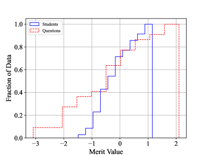
Figure 2: Empirical Cumulative Distribution of Merit Value. We analyze all students and questions under the Bradley-Terry-Luce model and show the empirical cumulative density function of inferred student abilities and question difficulties. The abilities ranges from -1.486 to 1.149 while the difficulties ranges from -3.090 to 2.099.

5.2 Algorithms

Simple Averaging

The grade for student $i$ is its average correctness on assigned questions. See the formal definition in Example 2.1.

Our Algorithm

The grade for student $i$ is an aggregation of the algorithm’s prediction on her performance on each question. All predictions can be classified into four cases, including existing edges (keep the fact as prediction), same component (maximum likelihood estimators), comparable components (answer in line with the path direction) and incomparable components (heuristic as simple averaging). See the formal definition in Section 3.2.

5.3 Ex-post Bias

5.3.1 Simulation 1: A Visualization of Simple Averaging’s Ex-post Unfairness

We compare the ex-post bias (Definition 6) between our algorithm and simple averaging given a fixed random task assignment graph. We use inferred parameters of all $35$ students and $22$ questions according to Figure 2. The task assignment graph is generated by Algorithm 1 with the parameter $m=22$ and $d=10$, i.e. each student is assigned 10 random questions from the whole question bank. The exam result graph is repeatedly generated according to the model.

Figure 3 shows the performance of two algorithms. The left plot corresponds to our algorithm and the right plot corresponds to simple averaging. In each plot, there are 35 confidence intervals, each corresponding to the difference between the student’s expected grade and her benchmark, i.e. $\mathbb{E}_{w}[\mathrm{alg}_{i}]-\mathrm{opt}_{i}$. The confidence intervals in the left plot are significantly closer to 0, compared to the right plot, which visualizes the intuition that students are facing different overall question difficulties under the random assignment and simple averaging fails to adjust their grades. Instead, our algorithm infers the question difficulties and the student abilities and adjusts their grades accordingly, largely reducing the ex-post bias.

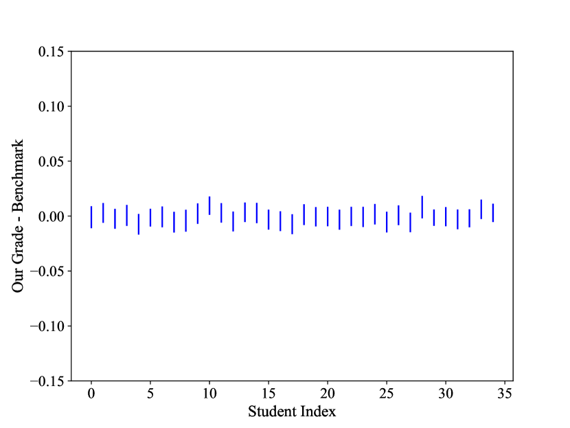
(a) Ex-post Grade Deviation of Our Algorithm

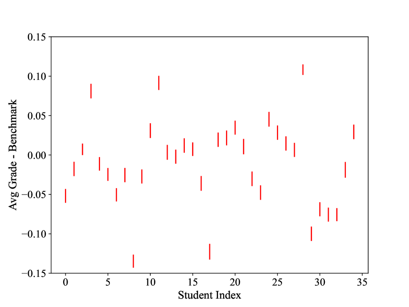
(b) Ex-post Grade Deviation of Simple Averaging

Figure 3: A Visualization of the Ex-post Grade Deviation with Degree Constraint $d=10$

5.3.2 Simulation 2: The Effect of the Degree Constraint

We compare the expected maximum ex-post bias, i.e., $\mathbb{E}_{G}\left[\max_{i\in S}\left(\mathbb{E}_{w}[\mathrm{alg}_{i}]-\mathrm{opt}_{i}\right)^{2}\right]$ and the expected average ex-post bias, i.e., $\mathbb{E}_{G}\mathbb{E}_{i\sim\mathcal{U}(S)}\left[\left(\mathbb{E}_{w}[\mathrm{alg}_{i}]-\mathrm{opt}_{i}\right)^{2}\right]$ between our algorithm and simple averaging. We use inferred parameters of all $35$ students and $22$ questions according to Figure 2. For each degree constraint $d$ from 1 to 22, we repeatedly generate task assignment graphs using algorithm Algorithm 1 with the other parameter $m=22$, i.e. each student is assigned $d$ independent questions from the whole question bank. For each task assignment graph, the exam result graph is repeatedly generated according to the model.

Figure 4 shows two algorithms’ expected maximum ex-post bias (Figure 4(a)) and expected average ex-post bias (Figure 4(b)) under different degree constraints, where our algorithm (blue curve) outperforms simple averaging (red curve) on every degree constraint $d$. Our algorithm’s expected ex-post bias with the degree constraint $d=5$ is close to simple averaging’s with the degree constraint $d=20$, which means our algorithm can ask 15 fewer questions to each student to achieve the same grading accuracy as simple averaging.

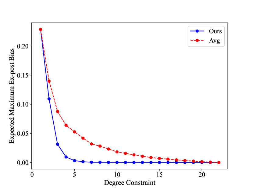
(a) Expected Maximum Ex-post Bias

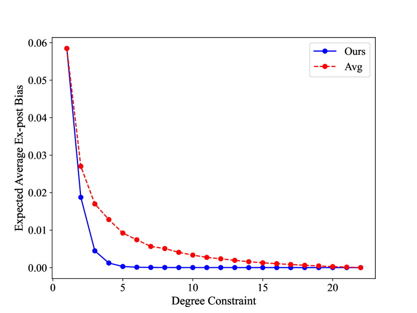
(b) Expected Average Ex-post Bias

Figure 4: Expected Aggregated Ex-post Bias v.s. Degree Constraint. The scale of expected average ex-post bias is about 4 times smaller than the scale of expected maximum ex-post bias.

We emphasize that our algorithm does not only perform better in expectation over random graphs but also on each of them. If we zoom in on a specific degree constraint, we can see two algorithms’ maximum ex-post bias and average ex-post bias on every task assignment graph. Figure 5 shows the case with the degree constraint $d=10$. Figure 5(a) corresponds to the maximum ex-post bias and Figure 5(b) corresponds to the average ex-post bias. In each case, the left plot contains 100 points, corresponding to a different task assignment graph, whose x-axis is the aggregated ex-post bias of simple averaging and whose y-axis is that of our algorithm; the right plot is the histogram of the difference in the aggregated ex-post bias between our algorithm and simple averaging. The simulation results show that our algorithm has a negligible aggregated ex-post bias compared to simple averaging on every task assignment graph.

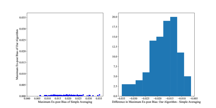
(a) Expected Maximum Ex-post Bias: 2.43e-4 for Our Algorithm and 1.80e-2 for Simple Averaging

(b) Expected Average Ex-post Bias: 4.08e-5 for Our Algorithm and 3.31e-3 for Simple Averaging

Figure 5: Aggregated Ex-post Bias on Task Assignment Graphs with Degree Constraint $d=10$

5.4 Ex-post Error and Bias-Variance Decomposition

In this part, we are investigating the expected average ex-post error (Definition 7), i.e.,
$\mathbb{E}_{G}\mathbb{E}_{i}\mathbb{E}_{w}[\left(\mathrm{alg}_{i}-\mathrm{opt}_{i}\right)^{2}]$. Through bias-variance decomposition, we relate the ex-post error to the ex-post bias and the variance in the algorithm performance.

Theorem 19 (Bias-Variance Decomposition).

$$\mathbb{E}_{G}\mathbb{E}_{i}\mathbb{E}_{w}[\left(\mathrm{alg}_{i}-\mathrm{opt}_{i}\right)^{2}]=\mathbb{E}_{G}\mathbb{E}_{i}[\left(\mathbb{E}_{w}[\mathrm{alg}_{i}]-\mathrm{opt}_{i}\right)^{2}]+\mathbb{E}_{G}\mathbb{E}_{i}\mathbb{E}_{w}[\left(\mathrm{alg}_{i}-\mathbb{E}_{w}[\mathrm{alg}_{i}]\right)^{2}].$$

Proof.

We prove a stronger argument of the decomposition for any fixed student $i$ and any fixed task assignment graph $G$,

$$\forall i,G,~{}\mathbb{E}_{w}[\left(\mathrm{alg}_{i}-\mathrm{opt}_{i}\right)^{2}]$$

$$= \mathbb{E}_{w}[\left(\mathrm{alg}_{i}-\mathbb{E}_{w}[\mathrm{alg}_{i}]+\mathbb{E}_{w}[\mathrm{alg}_{i}]-\mathrm{opt}_{i}\right)^{2}]$$

$$= \left(\mathbb{E}_{w}[\mathrm{alg}_{i}]-\mathrm{opt}_{i}\right)^{2}+\mathbb{E}_{w}[\left(\mathrm{alg}_{i}-\mathbb{E}_{w}[\mathrm{alg}_{i}]\right)^{2}]+2\mathbb{E}_{w}[\left(\mathrm{alg}_{i}-\mathbb{E}_{w}[\mathrm{alg}_{i}]\right)\left(\mathbb{E}_{w}[\mathrm{alg}_{i}]-\mathrm{opt}_{i}\right)]$$

$$= \left(\mathbb{E}_{w}[\mathrm{alg}_{i}]-\mathrm{opt}_{i}\right)^{2}+\mathbb{E}_{w}[\left(\mathrm{alg}_{i}-\mathbb{E}_{w}[\mathrm{alg}_{i}]\right)^{2}]+2\left(\mathbb{E}_{w}[\mathrm{alg}_{i}]-\mathrm{opt}_{i}\right)\mathbb{E}_{w}[\left(\mathrm{alg}_{i}-\mathbb{E}_{w}[\mathrm{alg}_{i}]\right)]$$

$$= \left(\mathbb{E}_{w}[\mathrm{alg}_{i}]-\mathrm{opt}_{i}\right)^{2}+\mathbb{E}_{w}[\left(\mathrm{alg}_{i}-\mathbb{E}_{w}[\mathrm{alg}_{i}]\right)^{2}].$$

∎

With the same setting in Section 5.3.1, we show the expected average ex-post error of our algorithm and simple averaging in Table 1. Our algorithm achieves a factor of 8 percent smaller ex-post error in total. But after the decomposition, we can see that our algorithm achieves a factor of 99 percent smaller ex-post bias with the cost of a factor of 10 percent larger variance. In practice, students will only take the exam once, so inevitably the variance of the algorithm would contribute to the total error. Our algorithm does not focus on how to reduce variance over the noisy answering process, instead, it focuses on the expected performance of the algorithm, i.e., it makes the ex-post bias much closer to zero. To verify that our algorithm does not increase the variance too much, we also run the simulation under “the worst case” of our algorithm, i.e., all students have the same abilities and all questions have the same difficulties. In this setting, our algorithm faces the risk of over-fitting, while simple averaging works perfectly. In Table 2, we can see that both algorithms achieve ex-post biases close to 0, and our algorithm has a factor of 1.6 percent larger variance than simple averaging which is the main contribution to the difference in ex-post errors.

	Ex-post Bias	Variance	Ex-post Error
Ours	0.00004	0.0188	0.0188
Avg	0.00331	0.0170	0.0203
Ours-Avg	-0.00327	0.0018	-0.0015

Table 1: Bias-Variance Decomposition in the setting of real-world parameters

	Ex-post Bias	Variance	Ex-post Error
Ours	0.0000500	0.0254	0.0255
Avg	0.0000493	0.0250	0.0250
Ours-Avg	0.0000007	0.0004	0.0005

Table 2: Bias-Variance Decomposition in the setting of all-the-same parameters

5.5 Real-World Data Experiment: Cross Validation

We cannot repeat an exam in the real world and check the ex-post bias of the algorithms. Thus, we sample part of the data we have as a new exam result graph and use them to predict the students’ actual average on the data. We randomly split the real-world data into training data and test data. Specifically, for a fixed student sample size $d_{1}$ and a degree constraint $d_{2}$, in each repetition, we randomly sample $d_{1}$ students and randomly choose $d_{2}$ questions and corresponding answers for each student independently as the training data, use our algorithm (Ours) and simple averaging (Avg) to predict every student’s average accuracy on the whole question bank, and calculate the mean squared error. Formally, the mean squared error $\mathrm{MSE}$ is defined as $\mathrm{MSE}=\mathbb{E}_{X,\tilde{S}}\left[\frac{1}{|\tilde{S}|}\sum_{i\in\tilde{S}}\left(\mathrm{alg}_{i}-\frac{1}{|Q|}\sum_{j\in Q}w_{ij}\right)^{2}\right],$ where $X$ is the training set given a fixed degree $d$, $\tilde{S}$ is the sampled student set, $\mathrm{alg}_{i}$ is student $i$’s grade given by the algorithm and $w_{ij}$ is the correctness of student $i$’s answer to question $j$. This measurement is closer to ex-post error except that the answering process is not repeatedly drawn.

In Figure 6(a), we fix the student sample size $d_{1}=35$, i.e., $\tilde{S}=S$ and change the degree constraint $d_{2}$ from 1 to $22$ and show the curve of the logarithm of $\mathrm{MSE}$. Our algorithm performs better than simple averaging when the degree constraint $d_{2}$ is larger than 5 and has a factor of 16% to 20% smaller MSE compared to simple averaging when the degree constraint $d_{2}$ is larger than 10. In Figure 6(b), we consider for every possible student sample size $d_{1}$, what the smallest degree constraints $d_{2}$ is for our algorithm to perform better than simple averaging. It provides a reference for choosing the grading rule in different situations.

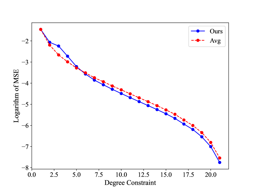
(a) Logarithm of MSE v.s. Degree Constraint

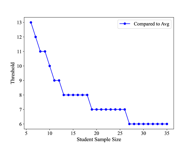
(b) Threshold v.s. Student Sample Size

Figure 6: Cross Validation

We also run the same cross-validation in numerical simulation. We assume two different Normal prior distributions for student abilities and question difficulties, fitted by the data in Figure 2. For a fixed student sample size $d_{1}$ and degree constraint $d_{2}$, in every repetition, we first draw $d_{1}$ i.i.d. student abilities and $|Q|=22$ i.i.d. question difficulties from those two prior distributions. We use a complete task assignment graph to generate the exam result graph according to the model. Then we randomly choose $d_{2}$ questions and the corresponding answers of each student as the training set and use our algorithm and simple averaging to predict each student’s average accuracy over the whole question bank. Note that we do exact same things in the cross-validation, so when calculating the MSE, we compare the algorithms’ grades to the students’ average accuracy given by the exam result graph instead of the benchmark. From Figure 7 we observe that the simulation result is quite similar to that of the real-world cross-validation, which suggests that the numerical simulation results we have in Section 5.3 and Section 5.4 could be a good reference for the practical use of our algorithm.

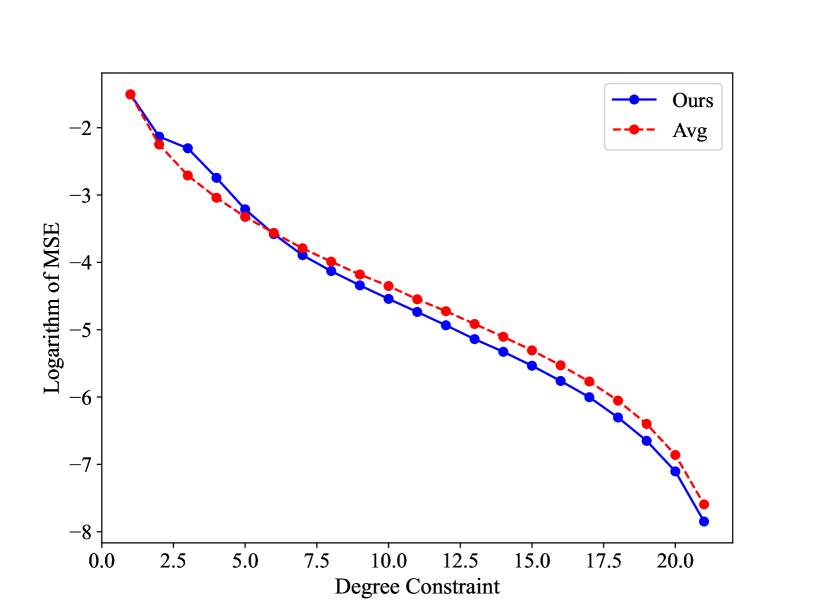
(a) Logarithm of MSE v.s. Degree Constraint

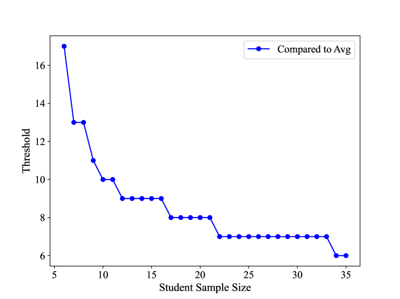
(b) Threshold v.s. Student Sample Size

Figure 7: Simulated Cross Validation

5.6 The Effect of the Question Sample Size (Exam Design Problem)

We now consider the infinite question bank and compare the expected maximum ex-post bias and the expected average ex-post bias between our algorithm and simple averaging. We sampled and fixed $|S|=5$ random students among the previous $35$ students. The question difficulties are i.i.d. distributed according to the linear interpolation of the difficulties shown in Figure 2. For each question sample size $m$, we repeatedly generate task assignment graphs using Algorithm 1 with the other parameter $d=5$. It can be expected that when $m=d$ and $m\to\infty$, two algorithms should have the same performance. Figure 8 shows a consistantly smaller expected maximum ex-post bias (Figure 8(a)) and expected average ex-post bias (Figure 8(b)) of our algorithm (blue curve) than simple averaging (red curve). As the question sample size grows, the expected aggregated ex-post bias of our algorithm first decreases and then increases. The turning point is about 6-9 for expected maximum ex-post bias and 10-15 for expected average ex-post bias.

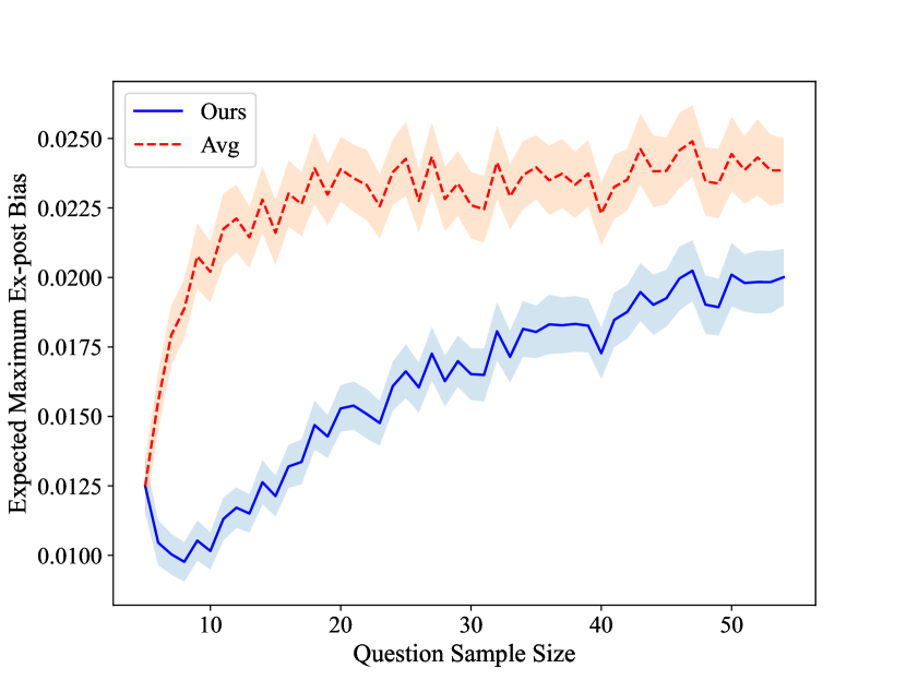
(a) Expected Maximum Ex-post Bias

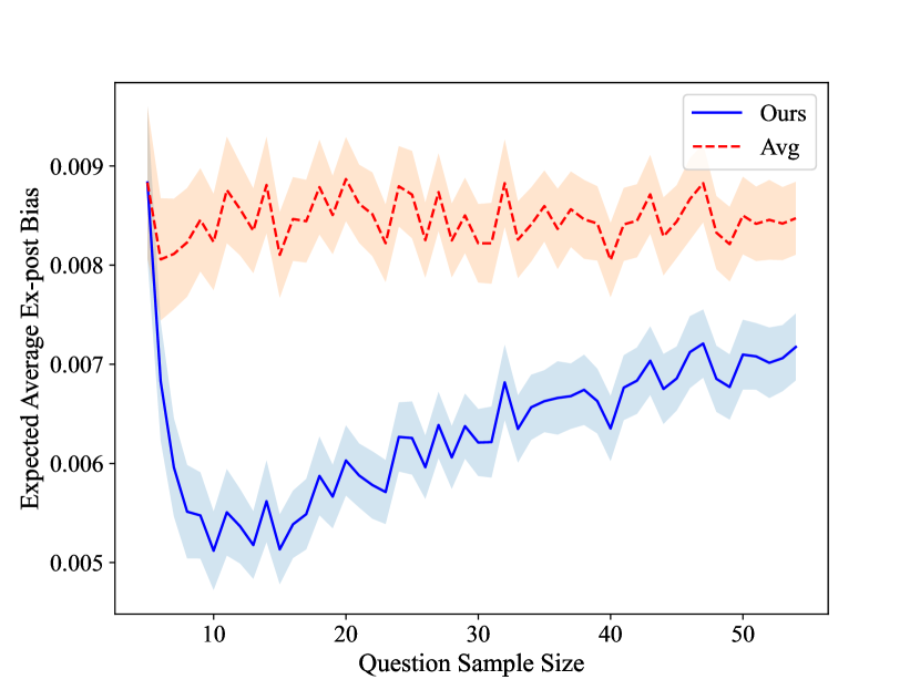
(b) Expected Average Ex-post Bias

Figure 8: Expected Aggregated Ex-post Bias v.s. Question Sample Size

6 Conclusions

We formulate and study the fair exam grading problem under the Bradley-Terry-Luce model. We propose an algorithm that is a generalization of the maximum likelihood estimation method. To theoretically validate our algorithm, we prove the existence, uniqueness, and uniform consistency of the maximum likelihood estimators under the Bradley-Terry-Luce model on sparse bipartite graphs. Our algorithm significantly outperforms simple averaging in numerical simulation. On real-world data, our algorithm is better when the students are assigned a sufficient number of questions (i.e., on sufficiently long exams). We provide guidelines for how to choose the grading rule given a certain number of students and a fixed exam length.

Our model in this paper mainly considers true-or-false questions, which can be extended to multiple-choice questions and to the case where it can be assumed that students would guess if they cannot solve a question. Our model treats student abilities and question difficulties as one-dimensional, which can be extended to a multi-dimensional model that takes different topics into account. Another potential extension of the model is to introduce different groups of students, so each question might have different difficulties for each group and we could ask for fairness across groups. Our method to treat missing edges across comparable components – which predicts 0 or 1 – needs to be improved, especially in the low-degree environment (i.e., short exam lengths where the exam result graph is unlikely to be strongly connected). Also, it would be important to provide a simple and clear explanation to students for practical use.

References

- An and Yung (2014) Xinming An and Yiu-Fai Yung. Item response theory: What it is and how you can use the irt procedure to apply it. SAS Institute Inc, 10(4):364–2014, 2014.
- Aziz (2020) Haris Aziz. Simultaneously Achieving Ex-ante and Ex-post Fairness, June 2020.
- Babaioff et al. (2022) Moshe Babaioff, Tomer Ezra, and Uriel Feige. Best-of-Both-Worlds Fair-Share Allocations, March 2022.
- Bechtel (1985) Gordon G. Bechtel. Generalizing the Rasch Model for Consumer Rating Scales. Marketing Science, 4(1):62–73, February 1985. ISSN 0732-2399. doi: 10.1287/mksc.4.1.62.
- Bezruczko (2005) Nikolaus Bezruczko. Rasch Measurement in Health Sciences. JAM Press, Maple Grove, Minn, 2005. ISBN 978-0-9755351-2-7 978-0-9755351-3-4.
- Bradley and Terry (1952) Ralph Allan Bradley and Milton E Terry. Rank analysis of incomplete block designs: I. the method of paired comparisons, 1952.
- De Alfaro and Shavlovsky (2014) Luca De Alfaro and Michael Shavlovsky. Crowdgrader: A tool for crowdsourcing the evaluation of homework assignments. In Proceedings of the 45th ACM technical symposium on Computer science education, pages 415–420, 2014.
- Enders (2010) Craig K. Enders. Applied Missing Data Analysis. Methodology in the Social Sciences. Guilford Press, New York, 2010. ISBN 978-1-60623-639-0.
- Ford (1957) L. R. Ford. Solution of a Ranking Problem from Binary Comparisons. The American Mathematical Monthly, 64(8):28–33, 1957. ISSN 0002-9890. doi: 10.2307/2308513.
- Fowler et al. (2022) Max Fowler, David H. Smith, Chinedu Emeka, Matthew West, and Craig Zilles. Are We Fair? Quantifying Score Impacts of Computer Science Exams with Randomized Question Pools. In Proceedings of the 53rd ACM Technical Symposium on Computer Science Education V. 1, SIGCSE 2022, pages 647–653, New York, NY, USA, February 2022. Association for Computing Machinery. ISBN 978-1-4503-9070-5. doi: 10.1145/3478431.3499388.
- Freeman et al. (2020) Rupert Freeman, Nisarg Shah, and Rohit Vaish. Best of Both Worlds: Ex-Ante and Ex-Post Fairness in Resource Allocation. In Proceedings of the 21st ACM Conference on Economics and Computation, EC ’20, pages 21–22, New York, NY, USA, July 2020. Association for Computing Machinery. ISBN 978-1-4503-7975-5. doi: 10.1145/3391403.3399537.
- Haberman (1977) Shelby J. Haberman. Maximum Likelihood Estimates in Exponential Response Models. The Annals of Statistics, 5(5):815–841, September 1977. ISSN 0090-5364, 2168-8966. doi: 10.1214/aos/1176343941.
- Haberman (2004) Shelby J. Haberman. Joint and Conditional Maximum Likelihood Estimation for the Rasch Model for Binary Responses. ETS Research Report Series, 2004(1):i–63, June 2004. ISSN 23308516. doi: 10.1002/j.2333-8504.2004.tb01947.x.
- Hamer et al. (2005) John Hamer, Kenneth T. K. Ma, Hugh H. F. Kwong, Kenneth T. K, Ma Hugh, and H. F. Kwong. A Method of Automatic Grade Calibration in Peer Assessment. In Of Conferences in Research and Practice in Information Technology, Australian Computer Society, pages 67–72, 2005.
- Han et al. (2020) Ruijian Han, Rougang Ye, Chunxi Tan, and Kani Chen. Asymptotic theory of sparse Bradley–Terry model. The Annals of Applied Probability, 30(5):2491–2515, October 2020. ISSN 1050-5164, 2168-8737. doi: 10.1214/20-AAP1564.
- Hunter (2004) David R. Hunter. MM algorithms for generalized Bradley-Terry models. The Annals of Statistics, 32(1), February 2004. ISSN 0090-5364. doi: 10.1214/aos/1079120141.
- Lee and Lee (2018) Won-Chan Lee and Guemin Lee. IRT Linking and Equating. In The Wiley Handbook of Psychometric Testing, chapter 21, pages 639–673. John Wiley & Sons, Ltd, 2018. ISBN 978-1-118-48977-2. doi: 10.1002/9781118489772.ch21.
- Moral and Rebollo (2017) Francisco J. Moral and Francisco J. Rebollo. Characterization of soil fertility using the Rasch model. Journal of soil science and plant nutrition, 17(2):486–498, June 2017. ISSN 0718-9516. doi: 10.4067/S0718-95162017005000035.
- Rasch (1993) Georg Rasch. Probabilistic Models for Some Intelligence and Attainment Tests. MESA Press, 5835 S, 1993. ISBN 978-0-941938-05-1.
- Raza et al. (2021) Syed A. Raza, Wasim Qazi, Komal Akram Khan, and Javeria Salam. Social Isolation and Acceptance of the Learning Management System (LMS) in the time of COVID-19 Pandemic: An Expansion of the UTAUT Model. Journal of Educational Computing Research, 59(2):183–208, April 2021. ISSN 0735-6331. doi: 10.1177/0735633120960421.
- Reily et al. (2009) Ken Reily, Pam Finnerty, and Loren Terveen. Two peers are better than one: Aggregating peer reviews for computing assignments is surprisingly accurate. In GROUP’09 - Proceedings of the 2009 ACM SIGCHI International Conference on Supporting Group Work, pages 115–124, January 2009. doi: 10.1145/1531674.1531692.
- Robitzsch (2021) Alexander Robitzsch. A Comprehensive Simulation Study of Estimation Methods for the Rasch Model. Stats, 4(4):814–836, December 2021. ISSN 2571-905X. doi: 10.3390/stats4040048.
- Sajjadi et al. (2016) Mehdi S. M. Sajjadi, Morteza Alamgir, and Ulrike von Luxburg. Peer Grading in a Course on Algorithms and Data Structures: Machine Learning Algorithms do not Improve over Simple Baselines, February 2016.
- Simons and Yao (1999) Gordon Simons and Yi-Ching Yao. Asymptotics when the number of parameters tends to infinity in the Bradley-Terry model for paired comparisons. The Annals of Statistics, 27(3):1041–1060, June 1999. ISSN 0090-5364, 2168-8966. doi: 10.1214/aos/1018031267.
- Waterbury (2019) Glenn Waterbury. Missing Data and the Rasch Model: The Effects of Missing Data Mechanisms on Item Parameter Estimation. Journal of applied measurement, 20:1–12, May 2019.
- Yan et al. (2012) Ting Yan, Yaning Yang, and Jinfeng Xu. Sparse Paired Comparisons in the Bradley-Terry Model. Statistica Sinica, 22(3):1305–1318, 2012. ISSN 1017-0405.
- Zermelo (1929) E. Zermelo. Die Berechnung der Turnier-Ergebnisse als ein Maximumproblem der Wahrscheinlichkeitsrechnung. Mathematische Zeitschrift, 29(1):436–460, December 1929. ISSN 0025-5874, 1432-1823. doi: 10.1007/BF01180541.