Importance is Important: A Guide to Informed Importance Tempering Methods

Abstract

Informed importance tempering (IIT) is an easy-to-implement MCMC algorithm that can be seen as an extension of the familiar Metropolis-Hastings algorithm with the special feature that informed proposals are always accepted, and which was shown in Zhou and Smith [51] to converge much more quickly in some common circumstances. This work develops a new, comprehensive guide to the use of IIT in many situations. First, we propose two IIT schemes that run faster than existing informed MCMC methods on discrete spaces by not requiring the posterior evaluation of all neighboring states. Second, we integrate IIT with other MCMC techniques, including simulated tempering, pseudo-marginal and multiple-try methods (on general state spaces), which have been conventionally implemented as Metropolis-Hastings schemes and can suffer from low acceptance rates. The use of IIT allows us to always accept proposals and brings about new opportunities for optimizing the sampler which are not possible under the Metropolis-Hastings framework. Numerical examples illustrating our findings are provided for each proposed algorithm, and a general theory on the complexity of IIT methods is developed.

Keywords: Informed proposals; Markov chain Monte Carlo sampling; multiple-try Metropolis; pseudo-marginal MCMC; simulated tempering; variable selection.

1 Introduction

1.1 Informed proposals and importance tempering

Let $\pi>0$ denote a posterior probability distribution on a discrete state space $\mathcal{X}$. A standard approach to approximating integrals with respect to $\pi$ is to run a Metropolis-Hastings (MH) algorithm, whose convergence rate largely depends on its proposal distributions. Throughout this paper, we fix a “reference” proposal scheme $q$; $q(y\,|\,x)$ denotes the probability of proposing $y$ given current state $x$. We generally assume that the computational cost for sampling from $q(\cdot\,|\,x)$ is negligible. We also assume that $q(x\,|\,x)=0$ for every $x$, and $q(x\,|\,y)>0$ whenever $q(y\,|\,x)>0$. For many discrete spaces, $q$ can be the random walk proposal such that $q(\cdot\,|\,x)$ is the uniform distribution on a set of states “close” to $x$. We call the MH algorithm equipped with the proposal $q$ the “uninformed” MH. Acceptance rates of uninformed MH schemes can be very low for high-dimensional problems arising in statistics and machine learning such as variable selection, graphical structure learning and deep neural networks. This leads to poor mixing and thus poor algorithmic efficiency.

Informed importance tempering (IIT) aims to ameliorate this problem by forcing the acceptance rate of the underlying Markov chain to be 1. In this work, we advocate for widespread adoption of the IIT framework. Though there are many details in the rest of this paper, the central argument is simple: it is straightforward to implement an IIT version of many MCMC algorithms, we can view IIT as a generalization of standard MH, and finally IIT is known to make substantial performance improvements in many statistically-relevant situations [51]. Much of this paper is concerned with giving details on how the IIT framework can be applied in different settings.

We now recall the main ideas leading to IIT. The primary motivation for IIT in [51] is to make efficient use of “informed proposals” [48], which adjust proposal weights of neighboring states according to their posterior probabilities. Define the “neighborhood” of $x$ by $\mathcal{N}_{x}=\{y\colon q(y\,|\,x)>0\}$; note $x\notin\mathcal{N}_{x}$. For each $y\in\mathcal{N}_{x}$, let $\alpha(x,y)\geq 0$ denote our “preference” for proposing $y$, which may depend on $\pi(y)$, and change its (un-normalized) proposal weight to $\eta(y\,|\,x)=q(y\,|\,x)\alpha(x,y)$; we call $\eta$ the weighting function. We restrict ourselves to considering the class of weighting functions introduced in Zanella [48], which takes the form

$$\eta_{h}(y\,|\,x)=q(y\,|\,x)\alpha_{h}(x,y),\quad\quad\alpha_{h}(x,y)=h\left(\frac{\pi(y)q(x\,|\,y)}{\pi(x)q(y\,|\,x)}\right),$$ (1)

where $h\colon(0,\infty)\rightarrow(0,\infty)$ satisfies $h(r)=rh(r^{-1})$ for any $r>0$. We say $h$ is a “balancing function” and the weighting function $\eta_{h}$ is “locally balanced.” Simple examples of balancing functions include $h(r)=\sqrt{r}$, $h(r)=1\wedge r$ and $h(r)=1\vee r$. If $y\notin\mathcal{N}_{x}$, we set $\eta_{h}(y\,|\,x)=0$, so $\eta_{h}(y\,|\,x)>0$ if and only if $q(y\,|\,x)>0$. Using $h(r)=rh(r^{-1})$, we find that

$$\pi(x)\eta_{h}(y\,|\,x)=\pi(y)\eta_{h}(x\,|\,y),\quad\quad\forall\,x,y\in\mathcal{X}.$$ (2)

A weighting function that satisfies (2) does not have to be locally balanced; an example is $\eta(y\,|\,x)=\pi(y)q(x\,|\,y)q(y\,|\,x)$. We direct readers to Zanella [48] for theoretical reasons why locally balanced schemes are preferred. Given $\eta_{h}$, we can define an informed proposal scheme, which is also said to be locally balanced, such that the proposal probability of $y$ given $x$ can be expressed by $\eta_{h}(y\,|\,x)/Z_{h}(x)$, where

$$Z_{h}(x)=\sum_{x^{\prime}\in\mathcal{N}_{x}}\eta_{h}(x^{\prime}\,|\,x)=\sum_{x^{\prime}\in\mathcal{N}_{x}}q(x^{\prime}\,|\,x)\alpha_{h}(x,x^{\prime})$$ (3)

is the normalizing constant. To implement informed proposals and calculate $Z_{h}(x)$, one needs to evaluate the posterior probability of each $x^{\prime}\in\mathcal{N}_{x}$ (in this paper, posterior evaluation always means to evaluate $\pi$ up to a normalizing constant), which is the main undesirable feature of informed MCMC methods, especially when parallel computing is not available.

For MH algorithms equipped with locally balanced proposals, the acceptance probability of the move $x\rightarrow y$ can be calculated by $\min\left\{1,Z_{h}(x)/Z_{h}(y)\right\}$. Zanella [48] theoretically showed that locally balanced MH algorithms yield nearly optimal performance (among all local MH schemes) for some high-dimensional problems such as weighted permutations and Ising models. For problems such as variable selection, Zhou et al. [52] showed that, surprisingly, locally balanced proposals could lead to exceedingly low acceptance rates that are even worse than uninformed MH algorithms, because the collinearity in the data can result in highly irregular behavior of the ratio $Z_{h}(x)/Z_{h}(y)$. They proposed an alternative informed proposal scheme and derived a mixing time bound for the corresponding MH algorithm.

A simpler solution to the problem of low acceptance rates is to use “importance tempering,” which essentially means to apply the importance sampling technique with Markov chain samples. Observe that, by (2), the transition matrix

$$\mathsf{P}_{h}(x,y)=\frac{\eta_{h}(y\,|\,x)}{Z_{h}(x)},\quad\forall\,x,y\in\mathcal{X},$$ (4)

is reversible with respect to the distribution $\pi_{h}$ such that $\pi_{h}(x)\propto\pi(x)Z_{h}(x)$. Hence, we can simulate the Markov chain $\mathsf{P}_{h}$ and calculate importance weights by $\pi(x)/\pi_{h}(x)\propto 1/Z_{h}(x)$. We will refer to $1/Z_{h}(x)$ as the importance weight of $x$ but note that it is un-normalized. This is the informed importance tempering (IIT) method proposed in Zhou and Smith [51], which is summarized in Algorithm 1 and is a generalization of the tempered Gibbs sampler (TGS) of Zanella and Roberts [49]. Given a function $f$, let $\pi(f)=\sum_{x\in\mathcal{X}}f(x)\pi(x)$. We can estimate $\pi(f)$ using the self-normalized importance sampling estimator

$$\hat{f}_{T}=\frac{\sum_{i=1}^{T}f(x^{(i)})w^{(i)}}{\sum_{i=1}^{T}w^{(i)}},$$ (5)

where $\{(x^{(i)},w^{(i)})\}_{i=1}^{T}$ is the output of Algorithm 1. For Algorithms 2 to 7 to be introduced in this paper, we will see that $w^{(i)}$ in the output is an unbiased estimator of the true un-normalized importance weight, and the same estimator of form (5) can be used.

Algorithm 1 Informed importance tempering (naive IIT)

Reference proposal $q$, balancing function $h$, number of iterations $T$, initial state $x^{(0)}$.

for $k=0,\dots,T$ do

     Set $x\leftarrow x^{(k)}$.

     Calculate $\eta_{h}(y\,|\,x)=q(y\,|\,x)\alpha_{h}(x,y)$ for every $y\in\mathcal{N}_{x}$.

     Calculate $Z_{h}(x)=\sum_{y\in\mathcal{N}_{x}}\eta_{h}(y\,|\,x)$.

     Set $w^{(k)}\leftarrow 1/Z_{h}(x)$.

     Draw $x^{(k+1)}\in\mathcal{N}_{x}$ from the distribution $\eta_{h}(\cdot\,|\,x)/Z_{h}(x)$.

end for

Samples $x^{(0)},x^{(1)},\dots,x^{(T)}$, un-normalized importance weights $w^{(0)},w^{(1)},\dots,w^{(T)}$.

1.2 Why importance weights are important

The main advantage of IIT is that it is often more efficient than both uninformed and informed MH algorithms. That is, the estimator $\hat{f}_{T}$ defined in (5) can converge much faster than the usual time-average estimator of an MH algorithm, even after one takes into account the per-iteration cost of IIT schemes. We give here a heuristic argument for why this occurs in the simple situation that $\pi$ is strongly unimodal and concentrates on one point $x^{\ast}$. Assume $h(r)=\sqrt{r}$. First, we expect the IIT chain to arrive at $x^{\ast}$ more quickly than MH, since IIT uses and always accepts informed proposals. Second, under the unimodal assumption, $1/Z_{h}(x^{\ast})$ is typically much larger than $1/Z_{h}(x)$ for any $x\neq x^{\ast}$, and thus $\hat{f}_{T}$ is likely to be very accurate as soon as the chain arrives at $x^{\ast}$. Combining these points, we expect IIT to converge more quickly. This heuristic was formalized and proved in [51], which showed that IIT is generally much more efficient than any MH algorithm with stationary distribution $\pi$ for a wide variety of statistically interesting problems, including variable selection, where we have posterior contraction.

A second advantage of IIT is that it is not difficult to implement or understand. Indeed, the familiar uninformed MH algorithm with proposal $q$ can be recast as an IIT-type scheme where only accepted moves are treated as samples and sojourn times are viewed as randomized importance weights [14, 24]. For the standard MH scheme, it is not difficult to see that the transition matrix of accepted moves is just $\mathsf{P}_{h}$ given in (4) with $h(r)=1\wedge r$. In this sense, IIT and uninformed MH use the same reference distribution and only differ in how they estimate the importance weights.

1.3 Overview of the paper

In this work, we develop new, general methodology of informed importance tempering, which improves the existing methods in terms of flexibility, applicability and efficiency.

First, IIT iterations are time-consuming due to the evaluation of $\pi$ in the entire neighborhood. Though IIT always leaves the current state in each iteration (which is a major advantage over MH schemes), using it at every state seems a waste of computational resources. We propose two strategies for reducing the computational cost of IIT schemes in Section 2. Algorithm 2 combines IIT updates with uninformed MH updates, and Algorithm 3 applies IIT to random neighborhood subsets. Numerical examples for variable selection in different scenarios are presented in Section 3. To compare the efficiency of uninformed MH and proposed methods, we need a unified theoretical framework for analyzing the convergence rates of importance-tempered MCMC samplers. We develop general theoretical results in Appendix A and provide a detailed analysis of Algorithm 2 in Section 4. Both the simulation study and theory illustrate that importance tempering enables us to devise more efficient MCMC algorithms that are not possible under the MH framework.

Second, we develop the methodology for efficiently combining IIT with other sophisticated MCMC schemes. When $\pi$ is severely multimodal, we can mimic the classical simulated tempering algorithm to allow the target to switch between a sequence of distributions with different degrees of flatness (i.e., at different temperatures); see Algorithms 4 and 5 in Section 5. After combining simulated tempering with IIT, one can choose the balancing function depending on the temperature so that that the sampler is encouraged to do more “exploitation” at low temperatures and more “exploration” at high temperatures, which is a unique advantage over classical tempering methods. An illustrative variable selection example is given in Section 5.3, where the posterior distribution has six local modes with very close posterior probabilities. In Section 6, we borrow the technique from pseudo-marginal MCMC methods [3] and propose an IIT scheme where $\pi(x)$ is replaced by an unbiased estimator of it; see Algorithm 6. This method can be very useful when the posterior evaluation of any state involves another intractable integral. In Section 6.2, we illustrate the use of our pseudo-marginal algorithm using a numerical example that arises from approximate Bayesian computation [28].

Third, the existing IIT methodology can only be applied to discrete state space. We propose Algorithm 7 in Section 7, which is applicable to general state spaces and resembles Algorithm 3 in that the informed proposal is used on random neighborhood sets. It turns out that Algorithm 7 is simply the importance-tempered version of the well-known multiple-try Metropolis (MTM) algorithm [31]. Again, our sampler, which accepts all proposals, has a significant advantage over some existing MTM methods that are known to suffer from low acceptance rates [46]. Our simulation study on multivariate normal targets shows that Algorithm 7 outperforms the recently proposed locally balanced MTM methods [11, 17]. Further, in Section 7.3, we apply Algorithm 7 to the record linkage analysis of a real data set investigated in Zanella [48]. The target is a joint distribution of one high-dimensional discrete variable and two continuous variables. Our algorithm outperforms the Metropolis-within-Gibbs sampler with either uninformed or informed MH updates.

1.4 Remarks on the proposed algorithms

We make three remarks on the proposed sampling schemes. First, in all of our numerical studies, we force each algorithm considered to use the same number of posterior calls, and thus IIT and informed MH schemes are run for much fewer iterations than uninformed MH. This is a conservative choice, showing IIT schemes in the worst possible light. In practice, informed sampling schemes are more amenable to parallelization than uninformed MH, which can further enhance the advantage of the proposed methods beyond what is demonstrated in this work. Second, the adjustments introduced in Algorithms 2 to 7 we propose are largely independent of each other. This means that one can easily combine all of the techniques that are useful for the problem at hand. Third, the construction of Algorithm 3, 6 and 7 relies on the following idea. We change the target distribution from $\pi(x)$ to a joint distribution $\pi(x,v)$ which has $\pi(x)$ as the marginal. Then, we construct a Markov chain on the joint state space which has stationary distribution $\tilde{\pi}(x,v)$, and calculate the un-normalized importance weight of $(x,v)$ by $C\pi(x,v)/\tilde{\pi}(x,v)$ for some constant $C>0$. The importance weight of $(x,v)$ can be thought of as an unbiased estimator of the true importance weight of $x$, since

$$\int\frac{C\pi(x,v)}{\tilde{\pi}(x,v)}\tilde{\pi}_{v\,|\,x}(v\,|\,x)\,\mathrm{d}v=\int\frac{C\pi(x,v)}{\tilde{\pi}(x)}\,\mathrm{d}v=C\frac{\pi(x)}{\tilde{\pi}(x)}.$$

Such use of auxiliary variables is common in the MCMC literature.

1.5 Other related works

The term “importance tempering” was coined by Gramacy et al. [19], which, broadly speaking, refers to estimating integrals with respect to $\pi$ using samples generated from an MCMC algorithm targeting a reference distribution $\tilde{\pi}$, an idea that dates back to Hastings [23]. But the focus of [19] was to apply this technique to the output of simulated tempering, where $\tilde{\pi}$ has the form $\tilde{\pi}(x)\propto\pi(x)^{a}$ for some $a>0$. Similar ideas have been used in a few other works [26, 43, 45, 2], where the reference distribution is $\pi^{a}$ or some other pre-specified approximation to $\pi$ (e.g. posterior distributions constructed by using the same likelihood function but different prior distributions). IIT differs from these works in that $\tilde{\pi}=\pi_{h}\propto\pi Z_{h}$, where the inverse importance weight $Z_{h}$ is “locally informed” in the sense that it contains information of the posterior landscape in the entire neighborhood; that is, we specify a local weighting scheme via $h$ rather than a global reference distribution. The motivation of IIT is also very different: we use it to force the acceptance probability of an informed proposal to equal one. Compared with importance sampling schemes where samples from $\tilde{\pi}$ are independently generated [40], a significant advantage of IIT is that one only needs to decide how to choose the balancing function $h$ instead of the whole reference distribution. Zhou and Smith [51] recommended the use of $h(r)=\sqrt{r}$, for which the induced reference distribution $\pi_{h}$ is guaranteed to act efficiently in a wide range of settings.

Other MCMC methods that utilize importance sampling include the Markov chain importance sampling algorithm [41, 39], which still runs an MH chain but makes use of rejected samples via importance sampling, and the dynamic weighting [32, 30], which uses importance weights to increase acceptance probabilities in MH algorithms on the fly. The most important difference between their approach and ours is the use of informed proposals, which was not considered in those works and can give a large advantage.

The idea of making proposals informed by the local posterior landscape can be found in many other MCMC methods, including the reduced-rejection-rate MH algorithm [6], applications of self-concordance [27], the Hamming ball sampler [44] and the adaptive proposal scheme proposed by Griffin et al. [20], though the term “informed proposal” was not used therein. As explained in Gagnon et al. [17], MTM is also informed in the sense that the sampler assigns informed proposal weights to a random set of candidate moves. The key difference between our approach and most existing informed methods is our use of importance tempering. Before the TGS sampler [49], the use of importance tempering with informed proposals, apparently, was only considered among the statistical physics community; see, e.g. the waiting time method of Dall and Sibani [12]. This work, as a continuation of [51], develops much more general algorithms which demonstrate that very often importance tempering, informed proposals and other MCMC sampling techniques can be combined easily and efficiently. Other promising ways to generalize IIT that are not considered in this work include devising non-reversible or adaptive IIT methods; the former has been studied in Power and Goldman [38] [c.f. 22], but its integration with the schemes proposed in this work remains to be explored.

Lastly, we note that the theory developed in this work is only for discrete spaces. On general spaces, the theory of importance tempering becomes much more involved, and different techniques may be needed; see, e.g., Andral et al. [2] and Franks and Vihola [16] for related theoretical results on general state spaces.

2 Fast informed importance tempering methods

Henceforth we will refer to Algorithm 1 as the naive IIT to distinguish it from the more sophisticated schemes to be proposed. Let $|\cdot|$ be the cardinality of a set. In each iteration of the naive IIT, we need to evaluate $\pi(y)/\pi(x)$ for every $y\in\mathcal{N}_{x}$. Even if we only consider local moves so that $|\mathcal{N}_{x}|\ll|\mathcal{X}|$, the set $\mathcal{N}_{x}$ can still be huge when the problem dimension is high. In this section, we propose two methods for generating informed proposals and estimating the importance weight $1/Z_{h}(x)$ without evaluating $\pi$ in the entire neighborhood $\mathcal{N}_{x}$.

2.1 Making use of uninformed Metropolis-Hastings updates

Assume the balancing function $h$ takes values in $[0,1]$. To estimate the importance weight of $x$, we can use the acceptance-rejection method. We repeatedly sample $y$ from $q(\cdot\,|\,x)$ and accept it with probability $\alpha_{h}(x,y)$. Denote by $W_{\rm{ar}}(x)$ the number of iterations until a successful proposal is made. Clearly, $W_{\rm{ar}}(x)$ is a geometric random variable with success probability $Z_{h}(x)$ defined in (3), which has mean $1/Z_{h}(x)$; thus, $W_{\rm{ar}}(x)$ is an unbiased estimator for the importance weight of $x$. Further, the accepted proposal has distribution $\mathsf{P}_{h}(x,\cdot)$.

As astute readers have noticed, if $h(r)=1\wedge r$, this acceptance-rejection method is just the uninformed MH algorithm equipped with proposal $q$. So uninformed MH is an importance tempering scheme where importance weights are estimated by geometric random variables (i.e., the number of iterations taken by the sampler to leave each state). Actually, other choices of $h$ still yield an MH scheme in the sense of Hastings [23]; see Remark 1.

Remark 1.

In the original work of Hastings [23], the acceptance rate was allowed to take a general form similar to $\alpha_{h}$ given in (1). Given any balancing function $h\in[0,1]$, we can construct an MH algorithm targeting $\pi$ and express its transition matrix by

$$\mathsf{P}_{\mathrm{mh}}(x,y)=\mathbbm{1}_{\{y\neq x\}}q(y\,|\,x)\alpha_{h}(x,y)+\mathbbm{1}_{\{y=x\}}\sum_{x^{\prime}\neq x}q(x^{\prime}\,|\,x)(1-\alpha_{h}(x,x^{\prime})),$$

where $\mathbbm{1}$ is the indicator function. The choice $h(r)=1\wedge r$ became prevalent largely because it was shown to be optimal for MH schemes [37], a result known as Peskun’s ordering. However, for IIT schemes, the optimal choice of $h$ largely depends on the problem, and very often $h(r)=1\wedge r$ is too conservative and thus sub-optimal [51]. Importance tempering brings about new challenges and opportunities for the optimal design of MCMC algorithms.

Remark 2.

The importance tempering perspective on the uninformed MH algorithms has been considered in the literature, and methods for reducing the importance weight estimator have been proposed [10, 5, 25, 14, 24]. These works consider general state spaces where exact calculation of the importance weight is not an option, and their methods either have limited application (e.g. can only be used for independence MH algorithms) or are computationally very expensive. Further, existing works only consider the special case $h(r)=1\wedge r$. The method we will propose in this section, though only for discrete spaces, is much more efficient and also straightforward to implement.

Remark 3.

The assumption $h\in[0,1]$ allows us to use the acceptance-rejection method, but it can be relaxed. If one has a balancing function $h$ bounded by a constant $C>0$, one can always consider $\tilde{h}(r)=h(r)/C$, which is still a balancing function. Further, importance sampling may be used. Given another reference distribution $\tilde{q}(\cdot\,|\,x)$, we can write $Z_{h}(x)=\sum_{x^{\prime}\in\mathcal{N}_{x}}\tilde{\eta}_{h}(x^{\prime}\,|\,x)\tilde{q}(x^{\prime}\,|\,x)$ where $\tilde{\eta}_{h}(x^{\prime}\,|\,x)=\eta_{h}(x^{\prime}\,|\,x)/\tilde{q}(x^{\prime}\,|\,x)$, and to estimate $1/Z_{h}(x)$ using acceptance-rejection, we only need to require that $\tilde{\eta}_{h}(\cdot\,|\,x)$ be bounded by a known constant.

Now we have two methods for estimating $1/Z_{h}(x)$: the exact calculation used by naive IIT and the acceptance-rejection method used by uninformed MH. The exact method always requires $|\mathcal{N}_{x}|$ posterior evaluations. The acceptance-rejection method, on average, requires $1/Z_{h}(x)$ posterior evaluations (one in each acceptance-rejection iteration). Consequently, when $|\mathcal{N}_{x}|<1/Z_{h}(x)$, the exact method has a smaller computational cost. To better see the distinction between the two methods, assume $h(r)=1\wedge r$ and $q(x\,|\,y)=q(y\,|\,x)$, and consider two extreme cases. First, suppose $\pi(y)\geq\pi(x)$ for every $y\in\mathcal{N}_{x}$. Then, $\alpha_{h}(x,y)=1$ for any $y\in\mathcal{N}_{x}$, and $Z_{h}(x)=1$. In this case, the acceptance-rejection method recovers the exact importance weight in only one iteration, and clearly there is no benefit in using the exact calculation. Second, suppose that $\pi(x)\gg\pi(y)$ for every $y\in\mathcal{N}_{x}$. Then $Z_{h}(x)$ can be extremely small, and the acceptance-rejection method becomes highly inefficient (i.e., the uninformed MH sampler gets stuck at $x$). In Bayesian statistics, such a scenario can easily happen when $x$ is the “true” value of the parameter and the data is sufficiently informative.

The above analysis shows that near local modes, we want to use the exact calculation, while the acceptance-rejection method may be preferred elsewhere. We propose a simple way to combine the two methods: in each iteration of the acceptance-rejection method, with probability $\rho$, we stop the iteration and perform an exact calculation, which adds $1/Z_{h}(x)$ to the current importance weight estimate (i.e., the number of completed acceptance-rejection iterations). This scheme is described in Algorithm A in detail. We further allow the exact update probability $\rho$ to depend on $x$, and the resulting importance tempering algorithm is given in Algorithm 2. To show Algorithm 2 is correct, it suffices to prove that Algorithm A yields an unbiased estimator for $1/Z_{h}(x)$ (see Appendix A).

Lemma 1.

Let $W(x)$ denote the importance weight estimate for state $x$ generated by Algorithm A with $\rho=\rho(x)$. Then, $\mathbb{E}[W(x)]=1/Z_{h}(x)$ and variance

$$\mathrm{Var}(W(x))=\frac{(1-Z_{h}(x))(1-\rho(x))}{Z_{h}(x)^{2}+\rho(x)Z_{h}(x)(1-Z_{h}(x))}.$$

Proof.

See Appendix B.1. ∎

Remark 4.

Observe that $\mathrm{Var}(W(x))$ is monotone decreasing with $\rho(x)$. When $\rho(x)=0$ (e.g., in an uninformed MH scheme), $\mathrm{Var}(W(x))=(1-Z_{h}(x))/Z_{h}(x)^{2}$, which is the variance of a geometric random variable with mean $1/Z_{h}(x)$. When $\rho(x)=1$, $\mathrm{Var}(W(x))=0$ since the importance weight is always calculated exactly.

Algorithm A Importance weight estimation

State $x$, reference proposal $q$, balancing function $h$, IIT update frequency $\rho$.

Set $y\leftarrow x$ and $w\leftarrow 0$.

while $y=x$ do

     Draw $U\sim\mathrm{Unif}(0,1)$.

     if $U\leq\rho$ then

         Calculate $\eta_{h}(y\,|\,x)=q(y\,|\,x)\alpha_{h}(x,y)$ for every $y\in\mathcal{N}_{x}$.

         Calculate $Z_{h}(x)=\sum_{y\in\mathcal{N}_{x}}\eta_{h}(y\,|\,x)$.                               $\left.\begin{array}[]{@{}c@{}}\\ {}\hfil\\ {}\hfil\\ {}\hfil\end{array}\right\}\begin{tabular}[]{l}IIT update\end{tabular}$

         Set $w\leftarrow w+1/Z_{h}(x)$.

         Draw $y\sim\eta_{h}(\cdot\,|\,x)/Z_{h}(x)$.

     else

         Set $w\leftarrow w+1$.

         Draw $y\sim q(\cdot\,|\,x)$ and calculate $\alpha_{h}(x,y)$.                        $\left.\begin{array}[]{@{}c@{}}\\ {}\hfil\\ {}\hfil\end{array}\right\}\begin{tabular}[]{l}MH update\end{tabular}$

         Set $y\leftarrow x$ with probability $1-\alpha_{h}(x,y)$.

     end if

end while

Importance weight estimate $w$ (for state $x$), and next state $y$.

Algorithm 2 Metropolis-Hastings-boosted informed importance tempering (MH-IIT)

Reference proposal $q$, balancing function $h\colon[0,\infty]\rightarrow[0,1]$, IIT update frequency $\rho\colon\mathcal{X}\rightarrow[0,1]$, number of iterations $T$, initial state $x^{(0)}$.

for $k=0,\dots,T$ do

     Set $(w^{(k)},x^{(k+1)})\leftarrow$ Algorithm A $(x^{(k)},q,h,\rho(x))$.

end for

Samples $x^{(0)},x^{(1)},\dots,x^{(T)}$, un-normalized importance weights $w^{(0)},w^{(1)},\dots,w^{(T)}$.

Consider Algorithm A with input $x,q,h,\rho$, and let $K(x)$ denote the (random) number of evaluations of $\pi$ in a single run of the algorithm (to be precise: we use the convention that each MH update requires one evaluation, and each IIT update requires $|\mathcal{N}_{x}|$ evaluations). A formula for the expected computational cost at state $x$, $\mathbb{E}[K(x)]$, is given in Lemma 2. We propose to use $\rho(x)=A/|\mathcal{N}_{x}|$, where $A$ is a fixed constant such that $0<A\leq\min_{x}|\mathcal{N}_{x}|$. Corollary 1 shows that, in terms of the computational cost, this choice of $\rho$ is “optimal” up to a constant factor.

Lemma 2.

Consider Algorithm A with $\rho=\rho(x)$. Then,

$$\mathbb{E}[K(x)]=\frac{\rho(x)(|\mathcal{N}_{x}|-1)+1}{\rho(x)(1-Z_{h}(x))+Z_{h}(x)}.$$

Proof.

See Appendix B.1. ∎

Corollary 1.

Let $\rho(x)=A/|\mathcal{N}_{x}|$ for some $A\in(0,\,\min_{x}|\mathcal{N}_{x}|\,]$. Then,

$$\mathbb{E}[K(x)]\leq\; \min\left\{\frac{A+1}{A}|\mathcal{N}_{x}|,\;\frac{A+1}{Z_{h}(x)}\right\}.$$

Remark 5.

For an uninformed MH scheme (i.e., $\rho\equiv 0$), we have $\mathbb{E}[K(x)]=1/Z_{h}(x)$, the expected sojourn time at $x$. For an IIT scheme (i.e., $\rho\equiv 1$), $\mathbb{E}[K(x)]=|\mathcal{N}_{x}|$. Choosing $A=1$, Corollary 1 shows that the computational cost of Algorithm A at any $x$ can be bounded by the minimum cost of IIT and uninformed MH schemes up to a factor of at most 2. Roughly speaking, this means that Algorithm A can automatically pick the more efficient method without a priori knowledge about the local posterior landscape.

2.2 Informed importance tempering with random neighborhood

When the neighborhood $\mathcal{N}_{x}$ is large, another natural idea for speeding up IIT iterations is to randomly sample a subset $\mathcal{S}\subseteq\mathcal{N}_{x}$ and make an informed proposal within $\mathcal{S}$. Let the size of this subset be $m$; we assume $m$ does not depend on $x$ and $2\leq m\leq\min_{x}|\mathcal{N}_{x}|$. Let

$$\mathfrak{N}(x,m)=\{\mathcal{S}\colon\mathcal{S}\subseteq\mathcal{N}_{x},|\mathcal{S}|=m\}$$

denote the collection of all subsets of $\mathcal{N}_{x}$ with size $m$. Recall that we assume $x\notin\mathcal{N}_{x}$, and thus $x\notin\mathcal{S}$ for any $\mathcal{S}\in\mathfrak{N}(x,m)$. Given $\mathcal{S}$, we sample the next state $y$ from $\mathcal{S}$ with probability proportional to $\eta_{h}(y\,|\,x)$, where $\eta_{h}$ is given by (1). That is, given $(x,\mathcal{S})$, the probability of moving to $y$ is given by $\eta_{h}(y\,|\,x)/Z_{h}(x,\mathcal{S})$, where

$$Z_{h}(x,\mathcal{S})=\sum_{x^{\prime}\in\mathcal{S}}\eta_{h}(x^{\prime}\,|\,x)=\sum_{x^{\prime}\in\mathcal{S}}q(x^{\prime}\,|\,x)\alpha_{h}(x,x^{\prime})$$

is the normalizing constant. The challenge is to design the sampling strategy of $\mathcal{S}$ such that the resulting stationary distribution of $(x,\mathcal{S})$ can be evaluated. It turns out that this can be achieved via a simple scheme described in Algorithm 3, where we use $\mathrm{Unif}(\mathcal{N},k)$ to denote the distribution of $k$ distinct states drawn from the set $\mathcal{N}$ with equal probability (i.e., uniform sampling without replacement). Note that, unlike in Algorithm 2, we allow $h$ to be unbounded.

Algorithm 3 Random neighborhood informed importance tempering (RN-IIT)

Reference proposal $q$, balancing function $h$, neighborhood subset size $m$, number of iterations $T$, initial state $x^{(0)}$, initial neighborhood $\mathcal{S}^{(0)}\in\mathfrak{N}(x^{(0)},m)$.

for $k=0,\dots,T$ do

     Set $x\leftarrow x^{(k)}$ and $\mathcal{S}\leftarrow\mathcal{S}^{(k)}$.

     Calculate $\eta_{h}(y\,|\,x)=q(y\,|\,x)\alpha_{h}(x,y)$ for every $y\in\mathcal{S}$.

     Calculate $Z_{h}(x,\mathcal{S})=\sum_{y\in\mathcal{S}}\eta_{h}(y\,|\,x)$.

     Set $w^{(k)}\leftarrow 1/(|\mathcal{N}_{x}|Z_{h}(x,\mathcal{S}))$.

     Draw $x^{(k+1)}\in\mathcal{S}$ from the distribution $\eta_{h}(\cdot\,|\,x)/Z_{h}(x,\mathcal{S})$.

     Draw $(y_{1},\dots,y_{m-1})$ from $\mathrm{Unif}(\mathcal{N}_{x^{(k+1)}}\setminus\{x\},m-1)$.

     Set $\mathcal{S}^{(k+1)}\leftarrow\{x,y_{1},\dots,y_{m-1}\}$.

end for

Samples $x^{(0)},x^{(1)},\dots,x^{(T)}$, un-normalized importance weights $w^{(0)},w^{(1)},\dots,w^{(T)}$.

Algorithm 3 defines a Markov chain on the augmented space $\mathcal{X}\times 2^{\mathcal{X}}$; denote its transition matrix by $\mathsf{P}_{\rm{rn}}$. For any $(x,\mathcal{S})$ and $(x^{\prime},\mathcal{S}^{\prime})$ such that $\mathcal{S}\in\mathfrak{N}(x,m)$, $\mathcal{S}^{\prime}\in\mathfrak{N}(x^{\prime},m)$, $x^{\prime}\in\mathcal{S}$ and $x\in\mathcal{S}^{\prime}$, we can write $\mathsf{P}_{\rm{rn}}((x,\mathcal{S}),(x^{\prime},\mathcal{S}^{\prime}))=\mathsf{P}_{\rm{rn}}(x^{\prime}\,|\,x,\mathcal{S})\mathsf{P}_{\rm{rn}}(\mathcal{S}^{\prime}\,|\,x,x^{\prime})$, where

$$\mathsf{P}_{\rm{rn}}(x^{\prime}\,|\,x,\mathcal{S})=\frac{q(x^{\prime}\,|\,x)\alpha_{h}(x,x^{\prime})}{Z_{h}(x,\mathcal{S})},\text{ and }\mathsf{P}_{\rm{rn}}(\mathcal{S}^{\prime}\,|\,x,x^{\prime})={\binom{|\mathcal{N}_{x^{\prime}}|-1}{m-1}}^{-1}.$$

The balancing property of function $h$ implies

$$\pi(x)Z_{h}(x,\mathcal{S})\mathsf{P}_{\rm{rn}}(x^{\prime}\,|\,x,\mathcal{S})=\pi(x^{\prime})Z_{h}(x^{\prime},\mathcal{S}^{\prime})\mathsf{P}_{\rm{rn}}(x\,|\,x^{\prime},\mathcal{S}^{\prime}).$$

Let $\pi(\mathcal{S}\,|\,x)$ be $\mathrm{Unif}(\mathcal{N}_{x},m)$. Observe that we can write

$$\mathsf{P}_{\rm{rn}}(\mathcal{S}^{\prime}\,|\,x,x^{\prime})=\frac{\pi(\mathcal{S}^{\prime}\,|\,x^{\prime})}{m/|\mathcal{N}_{x^{\prime}}|}.$$

It follows that $\mathsf{P}_{\rm{rn}}$ is reversible with respect to the distribution $\pi_{h}^{m}$ given by

$$\pi_{h}^{m}(x,\mathcal{S})\propto\frac{\pi(x)\pi(\mathcal{S}\,|\,x)}{w(x,\mathcal{S})},\text{ where }w(x,\mathcal{S})=\frac{m}{|\mathcal{N}_{x}|Z_{h}(x,\mathcal{S})}.$$ (6)

Letting $\pi(x,\mathcal{S})=\pi(x)\pi(\mathcal{S}\,|\,x)$ be our target distribution on the joint space, we see that $w(x,\mathcal{S})$ gives the importance weight of $(x,\mathcal{S})$. That is, Algorithm 3 is a naive IIT scheme that targets $\pi(x,\mathcal{S})$, which has $\pi$ as a marginal distribution. For many problems, $|\mathcal{N}_{x}|$ is a constant independent of $x$, in which case the un-normalized importance weight of $(x,\mathcal{S})$ simplifies to $1/Z_{h}(x,\mathcal{S})$; further, by setting $m=|\mathcal{N}_{x}|$, we obtain Algorithm 1. However, note that $m=1$ is not allowed in Algorithm 3. When we propose $(x^{\prime},\mathcal{S}^{\prime})$ from $(x,\mathcal{S})$, $\mathcal{S}^{\prime}$ is required to contain $x$, and if $m=1$, the algorithm will keep alternating between $x$ and $x^{\prime}$.

As discussed in Section 1.3, we can also think of $w(x,\mathcal{S})$ defined in (6) as an unbiased estimator for $1/Z_{h}(x)$, the (un-normalized) importance weight of $x$ in Algorithm 1.

Lemma 3.

Let $(x,\mathcal{S})\sim\pi_{h}^{m}$. The conditional expectation of $w(x,\mathcal{S})$ given $x$ is $1/Z_{h}(x)$.

Proof.

See Appendix B.1. ∎

We note that Algorithms A and 3, at least in theory, can be combined straightforwardly. If the function $h$ is bounded, one can invoke Algorithm A to estimate the importance weight $1/Z_{h}(x,\mathcal{S})$, which can be helpful when $m$ is still relatively large. Another important extension of Algorithm 3 is to generate the set $\mathcal{S}$ by sampling $m$ states from $\mathcal{N}_{x}$ according to $q(\cdot\,|\,x)$ with replacement. We will see in Section 7 that this generalization is closely related to MTM schemes and applies to general state spaces.

3 Simulation studies for variable selection targets

3.1 Three toy examples

We first consider three toy examples, where $\mathcal{X}=\{0,1\}^{p}$ and $\pi$ can be expressed in closed form. We let the uninformed proposal $q(\cdot\,|\,x)$ be the uniform distribution on $\mathcal{N}_{x}=\{y\colon\lVert x-y\rVert_{1}=1\}$, where $\lVert\cdot\rVert_{1}$ denotes the $\ell^{1}$-norm. We say $x\in\mathcal{X}$ is a local mode if $\pi(x)>\pi(y)$ for every $y\in\mathcal{N}_{x}$, and $\pi$ is unimodal if there is only one local mode. The three examples, despite being ideal and contrived, illustrate three typical scenarios in variable selection: $\pi$ is unimodal with independent coordinates in Example 1, unimodal with dependent coordinates in Example 2, and bimodal in Example 3. Explicit construction of the three variable selection problems is given in Appendix C.1.

For each example, we will introduce a discrete-valued function $F(x)$ and measure the convergence rates of MCMC samplers using $d(\pi,\hat{\pi}_{T};F)\in[0,2]$, which is defined by

$$d(\pi,\hat{\pi}_{T};F)=\sum_{k}\left|\pi(F^{-1}(k))-\hat{\pi}_{T}(F^{-1}(k))\right|,\quad F^{-1}(k)=\{x\colon F(x)=k\},$$ (7)

where the summation is over all possible values of $F$ and $\hat{\pi}_{T}$ is the (importance-weighted) empirical distribution of $T$ MCMC samples. That is, $d(\pi,\hat{\pi}_{T};F)$ is the total variation distance between the push-forward measures $\pi\circ F^{-1}$ and $\hat{\pi}_{T}\circ F^{-1}$. The closed-form expression of $\pi$ enables us to exactly calculate $d(\pi,\hat{\pi}_{T};F)$. We do not consider the total variation distance between $\pi$ and $\hat{\pi}_{T}$ since summation over $\mathcal{X}$ is not computationally feasible.

Example 1.

Let $p_{1}\in\{1,2,\dots,p\}$ and $x^{*}\in\mathbb{R}^{p}$ be given by $x^{*}_{i}=1$ if $i\leq p_{1}$ and $x^{*}_{i}=0$ if $i>p_{1}$. For $\theta>0$, define the target distribution by

$$\pi(x)=\frac{\mathrm{exp}(-\theta\lVert x-x^{*}\rVert_{1})}{\mathfrak{C}_{\theta}},\quad\text{ where }\mathfrak{C}_{\theta}=(1+e^{-\theta})^{p}.$$

Clearly, $\pi$ is unimodal with mode $x^{*}$, and $\pi$ has independent coordinates. This example represents an ideal variable selection problem where $x^{*}$ is the true model, all covariates in $x^{*}$ have equally strong effects, and the design matrix has orthogonal columns. The parameter $\theta$ controls the tail decay rate and indicates how strong the signals are. If one fixes $p$ and the true data-generating model, then $\theta\rightarrow\infty$ as the sample size tends to infinity; see Appendix C.1.

We fix $p=500$, set $F(x)=\lVert x-x^{*}\rVert_{1}$ and use simulation to find the number of posterior evaluations needed to achieve $d(\pi,\hat{\pi}_{T};F)\leq 0.1$. Figure 1 shows the results for 6 MCMC samplers when $p_{1}=50$: uninformed MH, Algorithms 1, 2, 3, locally balanced MTM of [11, 17] and weighted TGS of [49]. All samplers are initialized at $x^{(0)}=(0,\dots,0)$, and more details of their implementation are given in Appendix C.2. It can be seen from Figure 1 that when $\theta$ is small (i.e., $\pi$ is relatively flat), uninformed MH is the best, since it is efficient at exploring the whole space. When $\theta$ is large, naive IIT, MH-IIT and RN-IIT outperform uninformed MH due to the importance weighting. In particular, MH-IIT has the best performance among all methods. RN-IIT seems less efficient than naive IIT and MH-IIT in this scenario, but it is much better than the locally balanced MTM method, an MH algorithm with very similar dynamics. The wTGS sampler only performs well when $\theta$ is large, which can be partially explained by the theory developed in [51]; a detailed discussion is deferred to Appendix C.2. We have also tried the Hamming ball sampler of [44] and LIT-MH sampler of [52], but both methods performed poorly according our metric due to the high per-iteration computational cost (it could be beneficial to use these algorithms if parallel computing is available). Results for $p_{1}=20$ are given in Appendix C.2.

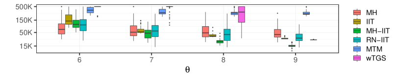
Figure 1: Box plot for the number of posterior calls needed to accurately approximate $\pi$ (see the main text) in Example 1 with $p=500$ and $p_{1}=50$. For each $\theta$, we repeat the simulation $50$ times. MH: uninformed MH; IIT: Algorithm 1; MH-IIT: Algorithm 2; RN-IIT Algorithm 3; MTM: the method of [11]; wTGS: the method of [49]. All samplers are forced to stop after $500$ thousand posterior calls.

Example 2.

For $\theta>0$, define $\pi(x)=\mathrm{exp}(-\theta\,\ell(x))/\mathfrak{C}_{\theta}$ where

$$\ell(x)=\left\{\begin{array}[]{cc}\lVert x\rVert_{1}-1,&\text{ if }x_{1}=1,\\ 2p-\lVert x\rVert_{1},&\text{ if }x_{1}=0,\end{array}\right.\quad\text{ and }\mathfrak{C}_{\theta}=\left(1+e^{-\theta(p+1)}\right)(1+e^{-\theta})^{p-1}.$$ (8)

It is not difficult to see that $\pi$ is unimodal with mode $x^{*}=(1,0,0,\dots,0)$, but $\pi$ has dependent coordinates. In variable selection, such a posterior distribution arises when only the first covariate has a nonzero effect but it is correlated with all the other covariates. See Appendix C.1.

For our simulation study, we use $p=500$ and define $F(x)=(\lVert x\rVert_{1}-1)\mathbbm{1}_{\{x_{1}=1\}}+p\mathbbm{1}_{\{x_{1}=0\}}$. Figure 2 shows the number of posterior calls needed to achieve $d(\pi,\hat{\pi}_{T};F)\leq 0.2$, when all samplers are initialized at the state $x^{(0)}$ such that $x^{(0)}_{i}=1$ if and only if $i>p-10$. Unlike in Example 1, we consider two MH-IIT schemes here: MH-IIT-1 uses $h(r)=1\wedge r$ (which was used in Example 1), and MH-IIT-2 uses the following balancing function with $c=2\theta$:

$$h_{c}(r)=(1\wedge re^{-c})\vee(r\wedge e^{-c}).$$ (9)

MH-IIT-1 is much more conservative than MH-IIT-2: if current state $x$ has $x_{1}=0$, $h(r)=1\wedge r$ assigns the same proposal weight to any $y\in\mathcal{N}_{x}$ such that $\lVert y\rVert_{1}=\lVert x\rVert_{1}+1$, while $h_{c}$ favors flipping $x_{1}$ since $h_{c}(r)=1\wedge re^{-c}$ for any $r\geq 1$; see Appendix C.3 for more discussion. As in Example 1, uninformed MH performs well only when $\theta$ is small. For large $\theta$, the posterior mass concentrates at the mode $x^{*}$, so the convergence of IIT schemes largely depends on when the first covariate is selected, making MH-IIT-2 much more efficient than MH-IIT-1. It should be emphasized that balancing functions such as $h_{c}$ are not desirable in MH schemes, because the acceptance probability for any neighboring state with smaller posterior (than the current one) is extremely low and thus the sampler needs to stay at a local mode for a huge number of iterations. However, this limitation is lifted in MH-IIT, and the optimal balancing function is no longer $h(r)=1\wedge r$; recall Remark 1. We acknowledge that the use of $c=2\theta$ is unrealistic as it requires knowledge about $\pi$, but we have observed that using any $c>\theta$ provides gains over MH-IIT-1. Another interesting observation is that RN-IIT is better than MH-IIT-1 in Figure 2, which is different from Example 1.

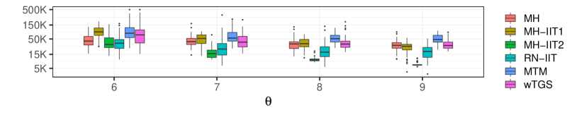
Figure 2: Box plot for the number of posterior calls (truncated at 500K) needed to accurately approximate $\pi$ in Example 2 with $p=500$. Each box represents $50$ runs. MH-IIT-1: Algorithm 2 with $h(r)=1\wedge r$; MH-IIT-2: Algorithm 2 with $h_{c}$ in (9). The other algorithms are the same as in Figure 1.

Example 3.

Let $p_{1}\in\{1,2,\dots,p\}$. Let $x_{(1)}^{*},x_{(2)}^{*}\in\mathcal{X}$ be given by $x_{(1)}^{*}=(1,0,1,\dots,1,0,\dots,0)$ and $x_{(2)}^{*}=(0,1,1,\dots,1,0,\dots,0)$ such that $\lVert x_{(1)}^{*}\rVert_{1}=\lVert x_{(2)}^{*}\rVert_{1}=p_{1}$. For $\theta>0$, define

$$\pi(x)=\frac{\mathrm{exp}(-\theta\lVert x-x_{(1)}^{*}\rVert_{1})+\mathrm{exp}(-\theta\lVert x-x_{(2)}^{*}\rVert_{1})}{\mathfrak{C}_{\theta}},\quad\text{ where }\mathfrak{C}_{\theta}=2(1+e^{-\theta})^{p}.$$ (10)

Clearly, $\pi$ is bimodal with local modes $x_{(1)}^{*},x_{(2)}^{*}$. This corresponds to a variable selection problem where the first two covariates are highly correlated.

We set $p=200$ in our simulation study, and let $F$ be the vector-valued function given by $F(x)=(\lVert x-x^{*}_{(1)}\rVert_{1},\lVert x-x^{*}_{(2)}\rVert_{1})$. Figure 3 shows the number of posterior calls needed to achieve $d(\pi,\hat{\pi}_{T};F)\leq 0.5$ for the six MCMC samplers considered in Example 1, initialized at $x^{(0)}=(0,\dots,0)$; see Appendix C.4 for details about the algorithms. The performance of uninformed MH quickly deteriorates as $\theta$ increases, while the performance of IIT methods seems relatively stable. A discussion on the performance of wTGS and the result for $p_{1}=20$ are given in Appendix C.4.

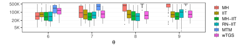
Figure 3: Box plot for the number of posterior calls (truncated at 500K) needed to accurately approximate $\pi$ in Example 3 with $p=200$ and $p_{1}=50$. Each box represents $50$ runs.

3.2 Simulation study with dependent designs

To mimic intricate real-world variable selection problems with correlated predictors, we employ the following simulation setting which is often considered in the literature [47, 52, 11]. First, we generate the design matrix $\bm{L}\in\mathbb{R}^{n\times p}$ with $n=1,000$ and $p=5,000$ by sampling each row independently from the multivariate normal distribution $N(0,\bm{\Sigma})$, where $\Sigma_{ij}=e^{-|i-j|}$. The response vector is generated by $\bm{Y}=\bm{L}\bm{\beta}+\bm{e}$, where $\bm{e}\sim N(0,\bm{I})$, $\beta_{j}=0$ if $j>20$, and for $j=1,\dots,20$, $\beta_{j}$ is drawn independently from $2\sqrt{(\log p)/n}\,\mathrm{Unif}\bigl{(}(2,3)\cup(-3,-2)\bigr{)}$. This is called the intermediate SNR (signal-to-noise ratio) case in Yang et al. [47]. The parameter of interest is $\bm{\gamma}\in\{0,1\}^{p}$, indicating which predictor variables are selected (i.e., have nonzero regression coefficients), and we calculate its posterior distribution $\pi$ in the same way as in [47, 52]. It has been shown in those works that $\pi$ tends to be highly multimodal in the intermediate SNR case, making the MCMC sampling challenging.

We consider nine MCMC samplers (see Appendix C.5 for details), all initialized at the same $\bm{\gamma}^{(0)}$ containing 10 randomly selected covariates, and run each sampler until $2.5\times 10^{6}$ posterior calls have been made. Denote by $\hat{\bm{\gamma}}$ the model with the highest posterior probability among all models visited by any of the samplers, and record the number of posterior calls taken by each sampler to find $\hat{\bm{\gamma}}$. We repeat this simulation 100 times, and show the results in Figure 4. The advantage of IIT methods over the others is quite significant. We suspect that uninformed MH is inefficient in this scenario largely because it can get trapped at local modes. As in Example 2, MH-IIT-2 is equipped with a more aggressive balancing function than MH-IIT-1, and probably due to the local dependence between the covariates, MH-IIT-2 performs better. Different from toy example studies, RN-IIT has the best performance in Figure 4, suggesting that it could be very useful for complex multimodal targets.

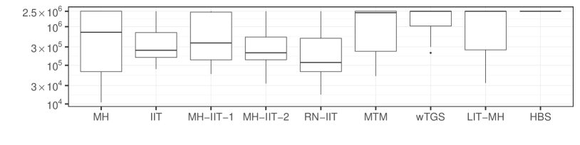
Figure 4: Box plot for the number of posterior calls (truncated at $2.5\times 10^{6}$) needed to find $\hat{\bm{\gamma}}$ in the variable selection simulation with $p=5,000$ and $n=1,000$. Each box represents $100$ replicates. Note that if the sampler fails to find $\hat{\bm{\gamma}}$, we set the number to $2.5\times 10^{6}$. LIT-MH: the method of [52]; HBS: the method of [44]. See Figures 1 and 2 for the name abbreviation of other algorithms.

4 Complexity analysis of Algorithm 2

In Appendix A, we develop a general theory on the complexity of importance tempering methods. To illustrate its use, we focus on Algorithm 2, MH-IIT, in this section. For whatever choice of the function $\rho$ in MH-IIT, the samples $(x^{(1)},\dots,x^{(T)})$ form a Markov chain with transition matrix $\mathsf{P}_{h}$ defined in (4), which has stationary distribution

$$\pi_{h}(x)=\frac{\pi(x)Z_{h}(x)}{\sum_{x}\pi(x)Z_{h}(x)}=\frac{\pi(x)Z_{h}(x)}{\pi(Z_{h})},$$

where we recall the notation $\pi(f)=\sum_{x\in\mathcal{X}}\pi(x)f(x)$. The expected computational cost at state $x$ (i.e., the expected number of posterior calls) is given by Lemma 2. Let $\kappa_{h,\rho}$ denote the expected cost averaged over the stationary distribution $\pi_{h}$. If $\rho\equiv c$ for some constant $c$, we simply write $\kappa_{h,c}$. A straightforward calculation gives

$$\kappa_{h,\rho}=\sum_{x\in\mathcal{X}}\pi_{h}(x)\mathbb{E}[K(x)]=\frac{1}{\pi(Z_{h})}\sum_{x\in\mathcal{X}}\frac{\pi(x)Z_{h}(x)\left[\rho(x)(|\mathcal{N}_{x}|-1)+1\right]}{\rho(x)(1-Z_{h}(x))+Z_{h}(x)}.$$

In particular, when $\rho\equiv 0$ and $\rho\equiv 1$, we have

$$\kappa_{h,0}=\sum_{x\in\mathcal{X}}\frac{\pi_{h}(x)}{Z_{h}(x)}=\frac{1}{\pi(Z_{h})},\quad\kappa_{h,1}=\sum_{x\in\mathcal{X}}\pi_{h}(x)|\mathcal{N}_{x}|\leq N_{\mathrm{max}},$$

where $N_{\mathrm{max}}=\max_{x}|\mathcal{N}_{x}|$ is the maximum neighborhood size. When $\rho$ is as given in Corollary 1, we denote it by $\rho=\rho(A)$ and find that

$$\kappa_{h,\rho(A)}\leq\min\left\{\frac{A+1}{A}\kappa_{h,1},\;(A+1)\kappa_{h,0}\right\}.$$

Hence if $A\geq 1$, the average computational cost of Algorithm 2 cannot exceed $(A+1)$ times that of uninformed MH or naive IIT schemes.

The complexity of MH-IIT also depends on the convergence rate of the importance sampling estimator $\hat{f}_{T}$ given by (5). Let $\sigma^{2}_{h,\rho}(f)$ denote the asymptotic variance of $\sqrt{T}\hat{f}_{T}$ as $T\rightarrow\infty$. We propose to measure the complexity of MH-IIT using $\kappa_{h,\rho}\sigma^{2}_{h,\rho}(f)$. When $\rho\equiv 0$, this is just the asymptotic variance of the time-average estimator produced from an uninformed MH algorithm. By a small abuse of notation, for $c\in[0,1]$ we write $\sigma^{2}_{h,c}$ in place of $\sigma^{2}_{h,\rho_{c}}$, where $\rho_{c}\equiv c$. For more details and a more general theory, see Appendix A.1. Our next theorem characterizes $\sigma^{2}_{h,\rho}(f)$, where $\mathrm{Gap}(\cdot)$ denotes the spectral gap of a transition matrix or a transition rate matrix.

Theorem 1.

Fix a balancing function $h\in[0,1]$ and suppose that $\mathrm{Gap}(\mathsf{P}_{h})<1$. For $f\colon\mathcal{X}\rightarrow\mathbb{R}$ with $\pi(f)=0$, define $\gamma(f)=\pi(Z_{h})\pi(f^{2}/Z_{h}).$ For any $\rho\colon\mathcal{X}\rightarrow[0,1]$, we have

1. $\sigma^{2}_{h,1}(f)\leq\sigma^{2}_{h,\rho}(f)\leq\sigma^{2}_{h,0}(f)\leq\sigma^{2}_{h,1}(f)+\gamma(f)$;

2. there exists $f^{*}$ with $\pi(f^{*})=0$ such that $\sigma^{2}_{h,1}(f^{*})\leq\sigma^{2}_{h,\rho}(f^{*})\leq 2\sigma^{2}_{h,1}(f^{*})$;

3. $\sigma^{2}_{h,\rho}(f)\leq 2\pi(f^{2})/\mathrm{Gap}(\mathsf{P}^{\mathrm{ct}}_{h})$ where the transition rate matrix $\mathsf{P}^{\mathrm{ct}}_{h}$ is given by

   $$\mathsf{P}^{\mathrm{ct}}_{h}(x,y)=\frac{\mathsf{P}_{h}(x,y)Z_{h}(x)}{\pi(Z_{h})},\quad\text{ if }x\neq y,$$

   and $\mathsf{P}^{\mathrm{ct}}_{h}(x,x)=-\sum_{x^{\prime}\neq x}\mathsf{P}^{\mathrm{ct}}_{h}(x,x^{\prime})$.

Proof.

See Appendix B.2. ∎

Remark 6.

By parts (i) and (ii), roughly speaking, the choice of $\rho$ does not have a significant impact on the asymptotic variance (at least for some function $f$). Hence, by part (iii), we can estimate the complexity of MH-IIT using

$$\mathrm{Comp}(h,\rho)=\frac{\kappa_{h,\rho}}{\mathrm{Gap}(\mathsf{P}^{\mathrm{ct}}_{h})}.$$ (11)

The use of a continuous-time Markov chain for studying importance sampling estimators was employed in Zanella and Roberts [49] for analyzing the TGS sampler and in Zhou and Smith [51] for analyzing the naive IIT sampler.

Example 2 (continued).

Consider Example 2 presented in Section 3.1 again. We fix $p=5$, choose the balancing function $h_{c}$ given by (9), and numerically calculate the complexity estimate defined in (11) for MH-IIT schemes. For simplicity, we only consider three choices of $\rho$: $\rho\equiv 0$ (uninformed MH), $\rho\equiv 1$ (naive IIT), and $\rho\equiv 0.5$. Results are shown in Table 1; see Appendix C.3 for plots. When $\theta=1$, uninformed MH is the best among the three choices of $\rho$, and when $\theta=3$, naive IIT is the best (reason was explained in Section 3.1). When $\rho\equiv 0$, the optimal choice of $c$ is always $c=0$, in which case $h_{c}$ is reduced to $h_{c}(r)=1\wedge r$; this is expected according to Peskun’s ordering. When $\rho\equiv 1$, $\kappa(\mathsf{P}_{h},\mathsf{R}_{h,\rho})$ is a constant, and thus the optimal choice of $c$ is the one that maximizes the spectral gap.

	$\theta=1$	$\theta=2$	$\theta=3$
$\max_{c\geq 0}\mathrm{Gap}(\mathsf{P}^{\mathrm{ct}}_{h})$	0.62 ($c=2.43$)	1.19 ($c=3.53$)	2.77 ($c=4.58$)
$\min_{c\geq 0}\mathrm{Comp}(h,\rho)$ with $\rho\equiv 0$	5.19 ($c=0$)	5.03 ($c=0$)	5.0 ($c=0$)
$\min_{c\geq 0}\mathrm{Comp}(h,\rho)$ with $\rho\equiv 1$	8.07 ($c=2.43$)	4.20 ($c=3.53$)	1.81 ($c=4.58$)
$\min_{c\geq 0}\mathrm{Comp}(h,\rho)$ with $\rho\equiv 0.5$	7.82 ($c=1.46$)	4.18 ($c=2.15)$	1.90 ($c=3.05$)

Table 1: Optimal complexity estimates for MH-IIT with balancing function $h_{c}$ in Example 2 with $p=5$. We numerically calculate $\mathrm{Gap}(\mathsf{P}^{\mathrm{ct}}_{h})$ and $\mathrm{Comp}(h,\rho)$ for different choices of $c$ and report the optimal values. Optimal choices of $c$ are given in parentheses. Minimum complexity in each column is highlighted in bold.

5 Tempering for multimodal targets

5.1 Informed importance tempering with constant temperature

In the narrow sense, “tempering” means to change the target distribution from $\pi$ to $\pi^{a}$ for some $a>0$ known as the inverse temperature. When $\pi$ has severe multimodality, this technique can be used to flatten the target distribution so that the sampler can move between the local modes more easily. To incorporate this technique, one can simply apply naive IIT by replacing $\pi$ with $\pi^{a}$, and correct for the bias when calculating the importance weight. The resulting algorithm is given in Algorithm 4, where we define

$$\eta_{h,a}(y\,|\,x)=q(y\,|\,x)h\left(\frac{\pi(y)^{a}q(x\,|\,y)}{\pi(x)^{a}q(y\,|\,x)}\right),\quad Z_{h,a}(x)=\sum_{x^{\prime}\in\mathcal{N}_{x}}\eta_{h,a}(x^{\prime}\,|\,x).$$

Algorithm 4 Constant-temperature informed importance tempering (CT-IIT)

Reference proposal $q$, inverse temperature $a>0$, balancing function $h$, number of iterations $T$, initial state $x^{(0)}$.

for $k=0,\dots,T$ do

     Set $x\leftarrow x^{(k)}$.

     Calculate $\eta_{h,a}(y\,|\,x)$ for every $y\in\mathcal{N}_{x}$.

     Calculate $Z_{h,a}(x)=\sum_{y\in\mathcal{N}_{x}}\eta_{h,a}(y\,|\,x)$.

     Set $w^{(k)}\leftarrow\pi^{1-a}(x)/Z_{h,a}(x)$. $\triangleright$ Up to a normalizing constant

     Draw $x^{(k+1)}\in\mathcal{N}_{x}$ from the distribution $\eta_{h,a}(\cdot\,|\,x)/Z_{h,a}(x)$.

end for

Samples $x^{(0)},x^{(1)},\dots,x^{(T)}$, un-normalized importance weights $w^{(0)},w^{(1)},\dots,w^{(T)}$.

It is easy to check that the samples generated from Algorithm 4 have stationary distribution $\pi_{h,a}(x)\propto\pi(x)^{a}Z_{h,a}(x)$. This results in the importance weight $\pi^{1-a}(x)/Z_{h,a}(x)$, which only needs to be evaluated up to a normalizing constant. When $h(r)=\sqrt{r}$, this scheme has been discussed in Zhou and Smith [51]. Algorithms 2 and 3 can be generalized analogously.

Example 4.

Consider $\mathcal{X}=\{0,1\}^{p}$. We modify Example 3 by letting

$$x_{(1)}^{*}=[\underbrace{1,1,0,0,1,\cdots,1,}_{p_{1}+2}0,\dots,0],\quad x_{(2)}^{*}=[0,0,\underbrace{1,1,1,\cdots,1,}_{p_{1}}0,\cdots,0],$$

and still defining $\pi$ by (10). Note $\lVert x_{(1)}^{*}\rVert_{1}=\lVert x_{(2)}^{*}\rVert_{1}=p_{1}$. We choose $p=200$ and $p_{1}=10$. This setting is more challenging than Example 3 since, to move between $x_{(1)}^{*}$ and $x_{(2)}^{*}$, the sampler needs to traverse some $x$ such that $\lVert x-x_{(1)}^{*}\rVert_{1}=\lVert x-x_{(1)}^{*}\rVert_{2}=2$. In the simulation, we use $h(r)=\sqrt{r}$, initialize Algorithm 4 at $x_{(1)}^{*}$, and count the number of iterations needed to reach $x_{(2)}^{*}$ at different temperatures (for any choice of $a$, the number of posterior calls per iteration is the same). Results are shown in Figure 5. Observe that the sampler exhibits poor performance when $a$ is either too small or too large. The naive IIT method without tempering (i.e., $a=1$) gets trapped around $x_{(1)}^{*}$ as $\theta$ increases, since the gap between the two modes becomes deeper. When $a$ is too small (i.e., the temperature is high), the sampler behaves like a random walk and fails to find the exact locations of the modes. This toy example shows that the optimal temperature needs to strike a balance between exploration and exploitation, but it may be difficult to find in practice.

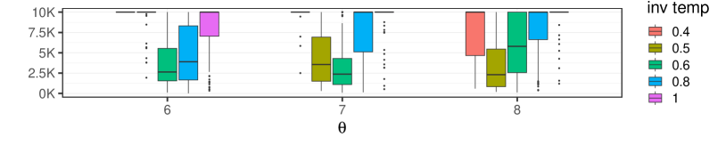
Figure 5: Box plot for the number of iterations (truncated at 10K) needed by Algorithm 4 to move from $x_{(1)}^{*}$ to $x_{(2)}^{*}$ in Example 4 with $p=200$ and $p_{1}=10$. Each box represents $100$ runs.

5.2 Informed importance tempering with varying temperature

In most existing tempering algorithms (e.g. parallel tempering and simulated tempering), a sequence of inverse temperatures $1=a_{0}\geq\cdots\geq a_{J}\geq 0$ is used so that the sampler can quickly explore multiple local modes at high temperatures (i.e., for large $j$) and pinpoint the positions of the modes at low temperatures (i.e., for small $j$). We now develop general informed importance tempering schemes whose dynamics mimic the simulated tempering algorithm [18, 36]. The main idea is to run a single-chain MCMC sampler with target distribution automatically switched between the tempered distributions $\pi^{a_{0}},\dots,\pi^{a_{J}}$.

Consider the augmented state space $\mathcal{X}\times\mathcal{J}$ with $\mathcal{J}=\{0,1,\dots,J\}$. Let $q_{\mathrm{st}}$ (subscript stands for “simulated tempering”) denote a proposal scheme on the joint space such that

$$q_{\mathrm{st}}(y,l\,|\,x,j)=\left\{\begin{array}[]{cc}q(y\,|\,x),&\text{ if }j=l,x\neq y,\\ q_{\mathrm{temp}}(l\,|\,j),&\text{ if }x=y,j\neq l,\\ 0,&\text{otherwise},\end{array}\right.$$

where $q_{\mathrm{temp}}(\cdot\,|\,j)$ denotes a proposal distribution on $\mathcal{J}$. So we never propose changing $x$ and $j$ simultaneously. Define $\mathcal{N}_{x,j}=\{(y,l)\colon q_{\mathrm{st}}(y,l\,|\,x,j)>0\}$. Let $\psi\colon\mathcal{J}\rightarrow(0,\infty)$ be a sequence of constants, $(h_{0},\dots,h_{J})$ be a sequence of balancing functions, $h^{*}$ be another balancing function, and define

$$\alpha_{\mathrm{st}}((x,j),(y,l))=\left\{\begin{array}[]{cc}h_{j}\left(\frac{\pi(y)^{a_{j}}\,q(x\,|\,y)}{\pi(x)^{a_{j}}\,q(y\,|\,x)}\right),&\text{ if }j=l,\vspace{0.2cm}\\ h^{*}\left(\pi(x)^{a_{l}-a_{j}}\frac{\psi(l)\,q_{\rm{temp}}(j\,|\,l)}{\psi(j)\,q_{\rm{temp}}(l\,|\,j)}\right),&\text{ if }x=y.\end{array}\right.$$ (12)

That is, $h_{j}$ is used to move between different states at temperature $1/a_{j}$ and $h^{*}$ is used to change the temperature. The resulting algorithm which combines IIT with simulated tempering is shown in Algorithm 5, where $\phi\colon\mathcal{J}\rightarrow(0,\infty)$ is another sequence of constants used to tune the weights of samples generated at different temperatures. We prove this algorithm correctly targets $\pi$ in Appendix B.3. It is worth noting that any choice of $\phi$ leads to a consistent importance sampling estimator as given by (5). The performance of these estimators can be better or worse than the simple choice $\phi(j)=\mathbbm{1}_{\{j=0\}}$, which only uses samples generated at temperature $1/a_{0}=1$. The optimal choice of $\phi$ was studied in depth in Gramacy et al. [19].

Algorithm 5 Varying-temperature informed importance tempering (VT-IIT)

Proposals $q$, $q_{\rm{temp}}$, inverse temperatures $\{a_{j}\}_{j=0}^{J}$, balancing functions $h^{*},\{h_{j}\}_{j=0}^{J}$, constants $\{\psi_{j}\}_{j=0}^{J}$, $\{\phi_{j}\}_{j=0}^{J}$, number of iterations $T$, initial state $x^{(0)}$ and index $j^{(0)}$.

for $k=0,\dots,T$ do

     Set $x\leftarrow x^{(k)}$, $j\leftarrow j^{(k)}$

     Calculate $\eta_{\mathrm{st}}(y,l\,|\,x,j)=q_{\mathrm{st}}(y,l\,|\,x,j)\alpha_{\mathrm{st}}((x,j),(y,l))$ for every $(y,l)\in\mathcal{N}_{x,j}$.

     Calculate $Z_{\mathrm{st}}(x,j)=\sum_{(y,l)\in\mathcal{N}_{x,j}}\eta_{\mathrm{st}}(y,l\,|\,x,j)$.

     Set $w^{(k)}\leftarrow\pi^{1-a}(x)\phi(j)/\{\psi(j)Z_{\mathrm{st}}(x,j)\}$. $\triangleright$ Up to a normalizing constant

     Draw $(x^{(k+1)},j^{(k+1)})\in\mathcal{N}_{x,j}$ from the distribution $\eta_{\mathrm{st}}(\cdot\,|\,x,j)/Z_{\mathrm{st}}(x,j)$.

end for

Samples $x^{(0)},x^{(1)},\dots,x^{(T)}$, un-normalized importance weights $w^{(0)},w^{(1)},\dots,w^{(T)}$.

The main motivation behind simulated tempering is to let high-temperature chains do the exploration and low-temperature ones do the exploitation. Our formulation using informed importance tempering allows us to achieve this much more efficiently, since the balancing function can be made temperature dependent. In particular, for high temperatures, we usually prefer using some conservative $h_{j}$ to encourage exploration, while for low temperatures, we want to let $h_{j}$ be aggressive. In an analogous way, we can mimic parallel tempering algorithms by running $J+1$ chains in parallel, which we do not further discuss in this work.

5.3 Simulation study on a multimodal example

We simulate one variable selection data set with $n=100,p=200$ as follows, which we expect yields six local modes in the posterior distribution. Denote the design matrix by $\bm{L}\in\mathbb{R}^{n\times p}$ and generate the response by $\bm{Y}=(\bm{L}_{1}+\bm{L}_{2}+\bm{L}_{3})\beta+N(0,0.5^{2}\bm{I}_{n})$, where $\bm{L}_{i}$ denotes the $i$-th column of $\bm{L}$ and $\beta=\sqrt{(\log p)/n}\times\mathrm{Unif}(4,6)$. Let $\bm{L}_{j}$ be generated from $N(0,\bm{I}_{n})$ for each $j$ except $j=4,5,8$. The posterior multimodality is introduced by setting

$$\bm{L}_{4}=\; \bm{L}_{2}-\bm{L}_{3}+N(0,0.1^{2}\bm{I}_{n}),$$

$$\bm{L}_{5}=\; \bm{L}_{1}+\bm{L}_{2}+\bm{L}_{3}+\bm{L}_{6}+\bm{L}_{7}+N(0,0.1^{2}\bm{I}_{n}),$$

$$\bm{L}_{8}=\; \bm{L}_{6}-\bm{L}_{7}+N(0,0.1^{2}\bm{I}_{n}).$$

Let $\mathcal{X}=2^{\{1,2,\dots,p\}}$, which is essentially the same as $\{0,1\}^{p}$ but now each $x\in\mathcal{X}$ indicates which covariates are selected. Six local modes are given by $\{1,2,3\}$, $\{1,2,4\}$, $\{1,3,4\}$, $\{5,6,7\}$, $\{5,6,8\}$, and $\{5,7,8\}$, and we denote them by $x^{*}_{(1)},\dots,x^{*}_{(6)}$, respectively. See Appendix D.1 for why these six models are of particular interest.

In the simulation study, we generate the temperature ladder by setting $a_{j}=(1+(j-1)\Delta)^{-1}$ for $j=0,1,\dots,J$, where $\Delta>0$ is some constant [19]. For balancing functions, we always use $h^{*}(r)=\min\{1,r\}$, but consider the following three schemes for choosing $\{h_{j}\}_{j=0}^{J}$.

$$\text{Method 1: }h_{j}(r)=1\wedge r\text{ for }j=0,1,\dots,J;$$

$$\text{Method 2: }h_{j}(r)=\sqrt{r}\text{ for }j<J/2,\text{ and }h_{j}(r)=1\wedge r\text{ for }j\geq J/2.$$

$$\text{Method 3: }h_{0}(r)=\sqrt{r}\text{ for }j=0,1,\dots,J-1,\text{ and }h_{J}(r)=1\wedge r.\$$

When Method 1 is used, Algorithm 5 is just the importance tempering version of the conventional simulated tempering algorithm. The choice of $\{\psi_{j}\}_{j=0}^{J}$ is described in Appendix D.1. For each sampler we consider, we initialize it at the null model $x^{(0)}=\emptyset$ , run it for $5\times 10^{4}$ iterations, and count how many distinct local modes out of $x^{*}_{(1)},\dots,x^{*}_{(6)}$ have been visited by the sampler. Results for 100 runs with $J=4$ are given in Table 2; for $J=9$, see Appendix D.1. Note that the six local modes can be divided into two groups, depending on whether the model involves the first four covariates. For the naive IIT sampler, it always finds one but only one group of local modes. In contrast, Algorithm 5 can efficiently jump between the two groups, when $\Delta$ and balancing functions are properly chosen. Notably, for both $\Delta=1$ and $\Delta=2$, Method 1 for choosing $\{h_{j}\}_{j=0}^{J}$ has the worst performance. This suggests that it is beneficial to use aggressive balancing functions at low temperatures, which, to our knowledge, has never been considered in the literature.

		$\Delta=1$			$\Delta=2$
No. local modes	IIT	M1	M2	M3	M1	M2	M3
3	100	87	83	75	12	1	4
4	0	1	1	0	2	1	1
5	0	3	0	2	5	3	6
6	0	9	16	23	81	95	89

Table 2: The number of distinct local modes (max=6) that have been visited by Algorithm 5 for the variable selection problem constructed in Section 5.3. Each column represents a sampler. IIT: Algorithm 1 without tempering. All the other samplers are Algorithm 5 with $J=4$, where $\Delta$ is the parameter in the temperature ladder and M1/M2/M3 denotes the three methods for choosing $\{h_{j}\}_{j=0}^{J}$ (see main text for details).

6 Pseudo-marginal informed importance tempering

6.1 Algorithm

When the evaluation of $\pi$ (up to a normalizing constant) involves another intractable integral, we may not be able to evaluate it exactly and only have access to some approximation denoted by $\hat{\pi}$. Such targets are said to be “doubly intractable” [35], and a natural idea is to replace $\pi$ with $\hat{\pi}$ in MCMC implementations. For MH algorithms, pseudo-marginal MCMC schemes can be used to sample from $\pi$ as long as $\hat{\pi}$ is unbiased [3]. It turns out that this technique can be applied to IIT schemes as well. We describe a pseudo-marginal version of Algorithm 1 in Algorithm 6. This algorithm differs slightly from the usual pseudo-marginal algorithm in that, in each iteration, we keep track of $(x,\hat{\pi}(x),\{\hat{\pi}(x^{\prime})\colon x^{\prime}\in\mathcal{N}_{x}\})$. When we move from $x$ to $y\in\mathcal{N}_{x}$ (note this implies $x\in\mathcal{N}_{y}$), the posterior estimates for $x$ and $y$ are not modified, and we only need to generate the posterior estimates for $y^{\prime}\in\mathcal{N}_{y}\setminus\{x\}$. Note also that an implementation can throw out all other estimates as the algorithm runs - they are always resampled before they are used. Assuming that $\hat{\pi}(x)=U_{x}\pi(x)$ for some strictly positive random variable $U_{x}$ whose distribution only depends on $x$ and has expectation equal to 1, we can prove Algorithm 6 correctly targets $\pi$; details are given in Appendix B.4. Algorithms 2 and 3 can be extended similarly.

In Appendix D.2, we apply Algorithm 6 to Example 2 by pretending that we only have unbiased estimates of posterior probabilities, and show that the use of importance tempering still provides a significant advantage over pseudo-marginal uninformed MH schemes.

Algorithm 6 Pseudo-marginal informed importance tempering (P-IIT)

Unbiased estimator $\hat{\pi}>0$, reference proposal $q$, balancing function $h$, number of iterations $T$, initial state $x^{(0)}$, posterior estimates $\hat{\pi}(x^{(0)})$ and $\hat{\pi}(y)$ for each $y\in\mathcal{N}_{x^{(0)}}$.

for $k=0,\dots,T$ do

     Set $x\leftarrow x^{(k)}$ and $\hat{\pi}(x)\leftarrow\hat{\pi}(x^{(k)})$.

     Calculate $\hat{\eta}_{h}(x^{\prime}\,|\,x)=q(x^{\prime}\,|\,x)h\left(\frac{\hat{\pi}(x^{\prime})q(x\,|\,x^{\prime})}{\hat{\pi}(x)q(x^{\prime}\,|\,x)}\right)$ for every $x^{\prime}\in\mathcal{N}_{x}$.

     Calculate $\hat{Z}_{h}(x)=\sum_{x^{\prime}\in\mathcal{N}_{x}}\hat{\eta}_{h}(x^{\prime}\,|\,x)$.

     Set $\hat{w}^{(k)}\leftarrow 1/\hat{Z}_{h}(x)$.

     Draw $y\in\mathcal{N}_{x}$ from the distribution $\hat{\eta}_{h}(\cdot\,|\,x)/\hat{Z}_{h}(x)$.

     Set $x^{(k+1)}\leftarrow y$.

     For each $y^{\prime}\in\mathcal{N}_{y}\setminus\{x\}$, generate $\hat{\pi}(y^{\prime})$.

     $\triangleright$ Note that $\hat{\pi}(x),\hat{\pi}(y)$ are not resampled. For any $x^{\prime}\in\mathcal{N}_{x}\setminus\{y\}$, $\hat{\pi}(x^{\prime})$ can be deleted.

end for

Samples $x^{(0)},x^{(1)},\dots,x^{(T)}$, estimated importance weights $\hat{w}^{(0)},\hat{w}^{(1)},\dots,\hat{w}^{(T)}$.

6.2 An example in approximate Bayesian computation

In approximate Bayesian computation, the target distribution, which we still denote by $\pi$ but is an approximation to the true posterior, is constructed by repeatedly simulating the data and comparing it to the observed data [34]. In general, $\pi$ is doubly intractable and pseudo-marginal MH schemes are often invoked to evaluate integrals with respect to $\pi$. A known issue of this approach is that, especially in the tails of $\pi$, the sampler can get stuck at some $x$ when we happen to generate some $\hat{\pi}(x)\gg\pi(x)$.

We study a toy example presented in Section 4.2 of Lee and Łatuszyński [28], where $\pi$ is a geometric distribution with success probability $1-ab$ for some $a,b\in(0,1)$. For each $x\in\{1,2,\dots,\}$, assume that we have access to some estimator $\hat{\pi}(x)$, which can be written as $\hat{\pi}(x)=\tilde{U}_{x}(1-a)a^{x-1}$, where $\tilde{U}_{x}$ is the mean of $K$ Bernoulli random variables with success probability $b^{x}$; see [29] for how this example arises from approximate Bayesian computation. We use simulation to study the performance of the pseudo-marginal uninformed MH algorithm and Algorithm 6 with $h(r)=\sqrt{r}$. The neighborhood of each $x$ is simply defined to be $\mathcal{N}_{x}=\{x-1,x+1\}$ if $x\geq 2$ and $\mathcal{N}_{x}=\{2\}$ if $x=1$. We set $a=0.5$, $b=0.4$ and $K=100$, initialize both samplers at $x^{(0)}=15$, and compare the estimation of the posterior mean $\sum_{x=1}^{\infty}x\,\pi(x)$. The left panel of Figure 6 shows the results when we discard first half of the samples as burn-in. We see that Algorithm 6 quickly produces a highly precise estimate, while the MH scheme requires a huge number of iterations to become roughly unbiased but the variance stays large even after $10^{5}$ iterations. If no samples are discarded (the right panel), Algorithm 6 is still much more efficient, but both samplers are slightly biased. It should be noted that because the auxiliary variable $\tilde{U}_{x}$ can be zero, Algorithm 6 is theoretically biased. We choose not to correct for this bias, since the bias is negligible (clearly in the left panel of Figure 6) and we find that it can significantly help stabilize the algorithm’s performance. A detailed explanation is given in Appendix D.3.

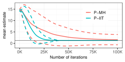
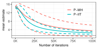
Figure 6: Estimate of the mean of $\pi$ for the geometric distribution example in Section 6.2. The solid colored lines represent the MCMC estimates, and dashed lines indicate $\pm 1$ standard deviation calculated from 50 runs. The black line indicates the true value, $(1-ab)^{-1}=1.25$. Left: half of samples discarded as burn-in when calculating the estimates; right: estimates calculated using all samples collected so far. P-MH: pseudo-marginal uninformed MH; P-IIT: Algorithm 6.

7 Multiple-try importance tempering

7.1 Algorithm

For the last method we introduce, we assume $\mathcal{X}$ is a general state space, and let $\pi(x),q(y\,|\,x)$ denote the density functions with respect to some dominating measure $\mu$. Let $\mathsf{Q}(x,A)=\int_{A}q(y\,|\,x)\mu(\mathrm{d}y)$. We still assume $\pi(x)>0$, $\mathsf{Q}(x,\{x\})=0$ for every $x$, and $q(x\,|\,y)>0$ whenever $q(y\,|\,x)>0$. The concept of the neighborhood $\mathcal{N}_{x}$ is no longer necessary, since it will not affect the implementation of the proposed method. For example, if $\mathcal{X}=\mathbb{R}$, $\mathsf{Q}(x,\cdot)$ can be a normal distribution with mean $x$. Using an idea similar to Algorithm 3, we can construct an IIT scheme for approximating $\pi$ on $\mathcal{X}$. There are two major differences. First, given current state $x$, we randomly draw $m$ candidates, $x_{1},\dots,x_{m}$, from $\mathsf{Q}(x,\cdot)$, which may not be distinct. Second, since the candidates are generated from $\mathsf{Q}(x,\cdot)$, we no longer include the term $q(x_{i}\,|\,x)$ when calculating the informed proposal weight of $x_{i}$; that is, the proposal weight of $x_{i}$ is set to $\alpha_{h}(x,x_{i})$ where $\alpha_{h}$ is defined in (1) for some balancing function $h$. The resulting algorithm is described in Algorithm 7, and its correctness is shown in Appendix B.5.

Algorithm 7 Multiple-try importance tempering (MT-IT)

Reference proposal $\mathsf{Q}$, balancing function $h$, neighborhood size $m$, number of iterations $T$, initial state $x^{(0)}$.

Set $\mathcal{S}^{(0)}\leftarrow(x^{(0)}_{1},\dots,x^{(0)}_{m})$, where $x^{(0)}_{i}$ is drawn from $\mathsf{Q}(x^{(0)},\cdot)$ for each $i$.

for $k=0,\dots,T$ do

     Set $x\leftarrow x^{(k)}$ and $\mathcal{S}\leftarrow\mathcal{S}^{(k)}$.

     Calculate $\alpha_{h}(x,y)$ for every $y\in\mathcal{S}$.

     Calculate $\tilde{Z}_{h}(x,\mathcal{S})=\sum_{y\in\mathcal{S}}\alpha_{h}(x,y)$.

     Set $w^{(k)}\leftarrow 1/\tilde{Z}_{h}(x,\mathcal{S})$.

     Draw $x^{(k+1)}\in\mathcal{S}$ from the distribution $\alpha_{h}(x,\cdot)/\tilde{Z}_{h}(x,\mathcal{S})$.

     Draw $y_{i}$ from $\mathsf{Q}(x^{(k+1)},\cdot)$ for $i=1,\dots,m-1$.

     Set $\mathcal{S}^{(k+1)}\leftarrow\{x,y_{1},\dots,y_{m-1}\}$.

end for

Samples $x^{(0)},x^{(1)},\dots,x^{(T)}$, un-normalized importance weights $w^{(0)},w^{(1)},\dots,w^{(T)}$.

One may have noticed that in Algorithm 7, the scheme for generating $x^{(k+1)}$ given $x^{(k)}$ is a special case of the proposal distribution used in classical MTM algorithms [31]. The main difference is that MTM algorithms are still MH schemes where an acceptance-rejection step is needed in every iteration, while Algorithm 7 always accepts the proposal and uses importance sampling to correct for the bias. We also note that the weighting functions considered in the early MTM literature do not take the form $\alpha_{h}$ given in (1), and it has been observed that MTM algorithms can suffer from low acceptance rates especially when $m$ is large [46]. The use of “locally balanced” weighting functions in MTM schemes can largely overcome this problem and has been studied in two recent works [11, 17]. But importance tempering seems a more efficient and reliable solution, since it guarantees that the chain never gets stuck at a single state no matter how $\pi$ behaves.

7.2 Simulation study with multivariate normal targets

We study a multivariate normal example investigated in Section 3 of Gagnon et al. [17]. The target distribution $\pi$ is chosen to be the standard $p$-variate normal distribution, $N(0,\bm{I}_{p})$. The proposal distribution $q(\cdot\,|\,x)$ is given by $N(x,\sigma^{2}\bm{I}_{p})$.

We consider two balancing functions, the square-root weighting $h(r)=\sqrt{r}$ and Barker’s weighting $h(r)=r/(1+r)$ [7, 33], both recommended by [17]. For each choice of $h$, we implement three methods, Algorithm 7 with fixed $\sigma$, MTM with fixed $\sigma$, and an adaptive version of MTM implemented in [17] where $\sigma$ is dynamically tuned. For all three methods, we fix the number of tries (i.e., parameter $m$ in Algorithm 7) equal to $50$, and for the two non-adaptive methods, we fix $\sigma=\sqrt{2.7/p^{0.75}}$, the initial value used in the adaptive method of [17]. It was reported in [17] that these two adaptive MTM schemes (which are said to be locally balanced) have superior performance to conventional “globally balanced” ones; see [48, 17] for details. We conduct simulation study with $p=50$ and all samplers initialized at $x^{(0)}=(10,\dots,10)$, which was the setting used in [17], and we find that Algorithm 7 performs even better. First, one major finding of [17] was that “globally balanced” MTM samplers can get stuck in low-posterior regions, while a locally balanced weighting scheme can help the sampler quickly move to high-posterior regions. The left panel of Figure 7 shows that importance tempering can further speed up the convergence: for both balancing functions, $\lVert x\rVert_{2}$ decreases much faster when importance tempering is used. Second, consider the estimation of $M_{2,p}=\int\lVert x\rVert_{2}^{2}\,\pi(\mathrm{d}x)$, of which the true value is equal to $p$. We run all samplers until $5\times 10^{5}$ posterior calls have been made, and use the last 50% of the samples to estimate $M_{2,p}$. The right panel of Figure 7 shows that for each balancing function, MT-IT yields most precise estimate, and the adaptive version with Barker’s weighting has a large bias. Results for estimation using last $10\%$ samples or all samples are given in Appendix D.4, from which similar observations can be made. An additional advantage of our method is that, since the chain is always moving, it is probably less sensitive to the choice of $\sigma$ than MTM methods, whose performance largely depends on the acceptance rate.

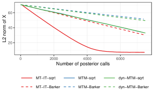
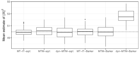
Figure 7: MTM methods targeting $N(0,\bm{I}_{p})$ with $p=50$. Left: trajectory of $\lVert x\rVert_{2}$ averaged over 100 runs (blue and green solid lines coincide). Right: box plot of the estimate of the mean of $\lVert x\rVert_{2}^{2}$ over 100 runs using half of the samples. MT-IT: Algorithm 7 with fixed proposal; MTM: MTM with fixed proposal [17]; dyn-MTM: adaptive MTM used in [17]; sqrt: $h(r)=\sqrt{r}$; Barker: $h(r)=r/(1+r)$.

7.3 A real data example on record linkage

Finally, we consider the application of the MT-IT algorithm to a bipartite record linkage problem studied in Zanella [48]. The data is available in the R package italy. Let $\bm{A}\in\mathbb{R}^{n_{1}\times K}$ and $\bm{B}\in\mathbb{R}^{n_{2}\times K}$ denote two data sets we have, denote by $\bm{a}_{i}$ the $i$-th row of $\bm{A}$, the vector representing the $i$-th record in the first data set, and denote by $\bm{b}_{i}$ the $i$-th row of $\bm{B}$. The same $K$ covariates are observed for both data sets. Let $M_{i}=j$ if $\bm{a}_{i}$ is matched with $\bm{b}_{j}$, and let $M_{i}=0$ if $\bm{a}_{i}$ is not matched with any record in the second data set. (“Matching” means that we believe the two records are duplicates.) Assume that any record is matched with at most one in the other data set. Hence, we can define $M^{-1}_{j}=i$ if $M_{i}=j$, and let $M^{-1}_{j}=0$ if $\bm{b}_{j}$ is not matched with anyone in the first data set. The parameter of interest is the $n_{1}$-dimensional vector $\bm{M}=(M_{1},\dots,M_{n_{1}})\in\{0,1,\dots,n_{2}\}^{n_{1}}$, and for each $\bm{M}$, we construct a neighborhood $\mathcal{N}_{\bm{M}}$ which has cardinality $n_{1}n_{2}$; see Appendix E.2 for details.

The goal is to generate samples from the joint posterior distribution $\pi(\bm{M},p_{\mathrm{match}},\lambda)$ considered in Zanella [48], where $p_{\mathrm{match}},\lambda$ are two continuous hyperparameters. A standard approach is to use the Metropolis-within-Gibbs sampler that alternates between direct sampling from $\pi(p_{\mathrm{match}},\lambda\,|\,\bm{M})$ and an MH scheme targeting $\pi(\bm{M}\,|\,p_{\mathrm{match}},\lambda)$. We implement two methods for updating $\bm{M}$: uninformed MH, and the blocked informed MH scheme of [48] with number of tries equal to $100$. We will simply refer to the two resulting Metropolis-within-Gibbs samplers as uninformed and informed MH, respectively. To mimic the dynamics of the informed MH sampler, we devise an MT-IT scheme using a mixture proposal distribution: given current state $(\bm{M},p_{\mathrm{match}},\lambda)$, with probability $\delta$ we propose a new value for $(p_{\mathrm{match}},\lambda)$ from its conditional distribution given $\bm{M}$, and with probability $1-\delta$ we propose a new value for $\bm{M}$ by uniformly sampling from $\mathcal{N}_{\bm{M}}$. We set $\delta=0.99$ and $m=100$. More details of the samplers are given in Appendix E.3.

The italy package contains the record data of 20 regions, and, for illustration purposes, we select region 4 since it has a relatively small sample size ($n_{1}=310,n_{2}=277$). It can be seen from Figure 8 that MT-IT outperforms both uninformed and informed MH. All three samplers seem to have converged after about $8\times 10^{5}$ posterior calls, but MT-IT is able to move to high-posterior regions more quickly than the other two. The advantage of MT-IT has also been observed for the other regions in the italy package, and more results are given in Appendix E.4. Note that though uninformed and informed MH have very similar performance in Figure 8, the actual number of iterations of informed MH is much smaller than that of uninformed MH (since we fix the total number of posterior calls). When parallel computing is available, both MT-IT and informed MH can be much more efficient.

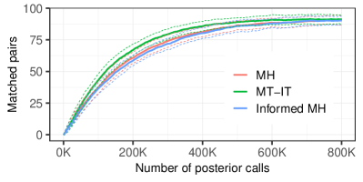
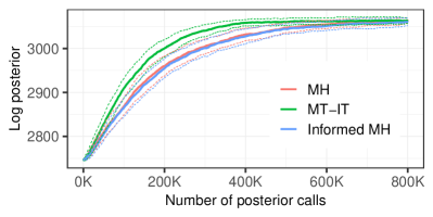
Figure 8: Results for the record linkage analysis of region 4 in the R package italy. Left panel: matched pairs, i.e., $\sum_{i=1}^{n_{1}}\mathbbm{1}\{M_{i}>0\}$. Right panel: log posterior probability. The solid colored lines represent the average values obtained from 50 runs, and dashed lines indicate $\pm 1$ standard deviation. All samplers target $\pi(\bm{M},p_{\mathrm{match}},\lambda)$ considered in [48]. MH: Metropolis-within-Gibbs sampler with uninformed MH updates; informed MH: Metropolis-within-Gibbs sampler with informed MH updates; MT-IT: Algorithm 7.

8 Discussion

The central theme of this work is to demonstrate that importance tempering is a more efficient framework for devising MCMC methods than traditional Metropolis-Hastings schemes. Two different perspectives on IIT are considered in this work, which are both useful. First, IIT can be seen as a generalization of MH schemes where we directly compute or estimate the sojourn time at each accepted state instead of using the acceptance-rejection procedure. This perspective has been utilized in a few existing works [14] and motivates the development of our Algorithm 2. Second, we can think of IIT as a technique that ensures the acceptance of a locally balanced proposal by modifying the target distribution. This view underlies the other algorithms proposed in this work. An immediate gain of using IIT is that it eliminates the issue of low acceptance rates. Further, the theory of [51] and our simulation studies show that the importance sampling estimators of IIT schemes are generally much more efficient than the estimators of MH schemes.

In our numerical examples, we assume parallel computing is unavailable and always match the total number of posterior calls of all algorithms considered, which is why we often see uninformed MH outperforms some informed MH schemes. However, notably, IIT schemes remain superior to uninformed MH in such settings. The advantage of IIT schemes over informed MH schemes seems quite significant, suggesting that informed proposals probably should always be integrated with importance tempering.

Many interesting theoretical questions and methodological extensions of the proposed algorithms deserve further investigations. Firstly, more theoretical guidance on the choice of the balancing function $h$ is needed. For naive IIT, this question has been studied in [51], but for more complicated IIT schemes, the optimal choice of $h$ is largely unclear. In particular, in a parallel or simulated tempering scheme such as Algorithm 5, using a more aggressive balancing function at low temperatures seems always beneficial for multimodal targets. Secondly, the choice of the parameter $m$ (the number of tries) in Algorithms 3 and 7 needs to be carefully studied, since it may have a substantial effect on the sampler’s efficiency. Similar questions have been investigated for pseudo-marginal MCMC methods [8, 42], and the theoretical tools developed in those works may be useful for understanding Algorithms 3 and 7. Finally, various variance-bounding techniques have been proposed for pseudo-marginal MH methods [28], and their application to IIT schemes remains to be explored.

Appendices

Appendix A Theoretical complexity analysis of informed importance tempering methods

A.1 Measuring complexity of importance tempering schemes

For our theoretical analysis, we consider the following setting. Let $\mathcal{X}$ be discrete and target distribution $\pi>0$. Let$((X_{i},W_{i}))_{i\in\mathbb{N}}$ be a bivariate Markov chain with state space $\mathcal{X}\times[0,\infty)$ and transition kernel

$$\mathsf{P}_{\mathrm{IT}}((x,w),(x^{\prime},\mathrm{d}w^{\prime}))=\tilde{\mathsf{P}}(x,x^{\prime})\mathsf{R}(x^{\prime},\mathrm{d}w^{\prime}),$$ (13)

where $\tilde{\mathsf{P}},\mathsf{R}$ are transition kernels that satisfy the following conditions.

Assumption 1.

$\tilde{\mathsf{P}}$ is irreducible and reversible with respect to a probability distribution $\tilde{\pi}>0$, and there exists a constant $c>0$ such that

$$\int_{0}^{\infty}w\,\mathsf{R}(x,\mathrm{d}w)=\frac{c\,\pi(x)}{\tilde{\pi}(x)},\quad\quad\forall\,x\in\mathcal{X}.$$

Remark 7.

We say $\mathsf{P}_{\mathrm{IT}}$ is the transition kernel of an importance tempering scheme targeting $\pi$. For Algorithm 1, $\tilde{\mathsf{P}}=\mathsf{P}_{h}$ where $\mathsf{P}_{h}$ is given by (4), $\tilde{\pi}\propto\pi Z_{h}$ where $Z_{h}$ is given by (3), and $\mathsf{R}(x,\cdot)$ is a degenerate distribution that assigns unit probability to $1/Z_{h}(x)$. As we discussed in Section 2.1, uninformed MH schemes also have this bivariate Markov chain representation with $\tilde{\mathsf{P}}=\mathsf{P}_{h}$ and $\mathsf{R}(x,\cdot)$ being a geometric distribution with mean $1/Z_{h}(x)$; see Example 5 later. For Algorithm 2, $\tilde{\mathsf{P}}=\mathsf{P}_{h}$, and $\mathsf{R}(x,\cdot)$, by Lemma 1, satisfies Assumption 1. Note that under Assumption 1, $\mathsf{P}_{\mathrm{IT}}$ is always Harris recurrent.

Given a function $f$, denote its expectation with respect to $\pi$ by $\pi(f)=\sum_{x}\pi(x)f(x)$, and define the importance sampling estimator for $\pi(f)$ by

$$\hat{f}_{T}(\tilde{\mathsf{P}},\mathsf{R})=\frac{\sum_{i=1}^{T}f(X_{i})W_{i}}{\sum_{i=1}^{T}W_{i}},$$ (14)

where $T$ denotes the number of samples. Denote the collection of “centered” functions by

$$L_{0}^{2}(\mathcal{X},\pi)=\{f\colon f\text{ is a mapping from $\mathcal{X}$ to $\mathbb{R}$},\;\pi(f)=0,\;\pi(f^{2})<\infty\}.$$

For $f\in L_{0}^{2}(\mathcal{X},\pi)$, by a routine argument that applies the central limit theorem for the bivariate Markov chain $((X_{i},W_{i}))_{i\in\mathbb{N}}$ and Slutsky’s theorem (see, e.g. Proposition 5 in [13]), we find that

$$\sqrt{T}\hat{f}_{T}\overset{\mathrm{Law}}{\longrightarrow}N(0,\sigma^{2}(f;\tilde{\mathsf{P}},\mathsf{R})),$$

where $\sigma^{2}(f;\tilde{\mathsf{P}},\mathsf{R})$ is called the asymptotic variance of the estimator $\hat{f}_{T}$. Asymptotic variances are commonly used in the MCMC literature to measure the efficiency of samplers.

To derive a practically useful complexity metric for importance tempering schemes, we need to take into account the computational cost for simulating the kernel $\mathsf{P}_{\mathrm{IT}}$, which can vary widely across different algorithms. Since $X_{i+1}\sim\tilde{\mathsf{P}}(X_{i},\cdot)$ and $W_{i}\sim\mathsf{R}(X_{i},\cdot)$, we may assume that the computational cost for generating $(X_{i+1},W_{i})$ only depends on the value of $X_{i}$. Hence, we denote by $\kappa(x;\tilde{\mathsf{P}},\mathsf{R})$ the cost of simulating a pair $(X,W)$ where $X\sim\tilde{\mathsf{P}}(x,)$ and $W\sim\mathsf{R}(x,\cdot)$. Our formalism allows $\kappa$ to be any function of $x$, but in practice we will typically choose this to be the expected number of times that the posterior is evaluated (up to a normalizing constant) during each step of the algorithm. Let

$$\kappa(\tilde{\mathsf{P}},\mathsf{R})=\sum_{x\in\mathcal{X}}\tilde{\pi}(x)\kappa(x;\tilde{\mathsf{P}},\mathsf{R})$$ (15)

denote the cost averaged over $\tilde{\pi}$. We use $\sigma^{2}(f;\tilde{\mathsf{P}},\mathsf{R})\kappa(\tilde{\mathsf{P}},\mathsf{R})$ to measure the complexity of the importance tempering scheme $\mathsf{P}_{\mathrm{IT}}$, which we think of as the effective computational cost of each independent sample from $\pi$.

Example 5 (Relationship to Theory for Uninformed MH).

Consider the uninformed MH algorithm with transition matrix given by

$$\mathsf{P}_{\mathrm{mh}}(x,y)=\mathbbm{1}_{\{y\neq x\}}q(y\,|\,x)\alpha_{h}(x,y)+\mathbbm{1}_{\{y=x\}}\sum_{x^{\prime}\neq x}q(x^{\prime}\,|\,x)(1-\alpha_{h}(x,x^{\prime})),$$

where we allow $h$ to be any balancing function taking value in $[0,1]$ (the dependence of $\mathsf{P}_{\mathrm{mh}}$ on $h$ is omitted). Let $(Y_{1},Y_{2},\dots,)$ denote a trajectory of the MH sampler. Then $T^{-1/2}\sum_{i=1}^{T}f(Y_{i})$ converges in distribution to $N(0,\sigma^{2}_{\mathrm{mh}}(f))$, where $\sigma^{2}_{\mathrm{mh}}(f)$ denotes the corresponding asymptotic variance. If we rewrite it as an importance tempering scheme (i.e., $X_{i}$ is the $i$-th accepted state and $W_{i}$ is the number of iterations the MH sampler stays at $X_{i}$), then the pair $(\tilde{\mathsf{P}},\mathsf{R})$ is given by

$$\tilde{\mathsf{P}}_{\mathrm{mh}}(x,y)=\mathbbm{1}_{\{y\neq x\}}\frac{q(y\,|\,x)\alpha_{h}(x,y)}{Z_{h}(x)},\quad\mathsf{R}_{\mathrm{mh}}(x,\cdot)=\mathrm{Geom}(Z_{h}(x)),$$

where $Z_{h}(x)=\sum_{x^{\prime}\neq x}q(x^{\prime}\,|\,x)\alpha_{h}(x,x^{\prime})$. Since each uninformed MH iteration requires one posterior evaluation (for the proposed state), we have $\kappa(x;\tilde{\mathsf{P}}_{\mathrm{mh}},\mathsf{R}_{\mathrm{mh}})=1/Z_{h}(x)$, the expected number of iterations needed to leave $x$. Recall that the stationary distribution of $\tilde{\mathsf{P}}_{\mathrm{mh}}$ is given by $\pi_{h}(x)=\pi(x)Z_{h}(x)/\pi(Z_{h})$, and it follows that

$$\kappa(\tilde{\mathsf{P}}_{\mathrm{mh}},\mathsf{R}_{\mathrm{mh}})=\sum_{x}\frac{\pi(x)Z_{h}(x)}{\pi(Z_{h})}\frac{1}{Z_{h}(x)}=\frac{1}{\pi(Z_{h})}.$$

Note that $\pi(Z_{h})^{-1}$ is the simply the expectation of $W(X)\sim\mathsf{R}_{\mathrm{mh}}(X,\cdot)$ where $X\sim\pi_{h}$. Since $\sigma^{2}(\tilde{\mathsf{P}}_{\mathrm{mh}},\mathsf{R}_{\mathrm{mh}})$ is the asymptotic variance of

$$\sqrt{N}\frac{\sum_{i=1}^{N}f(X_{i})W_{i}}{\sum_{i=1}^{N}W_{i}}=\frac{\sum_{i=1}^{T_{N}}f(Y_{i})}{\sqrt{T_{n}}}\frac{1}{\sqrt{(\sum_{i=1}^{N}W_{i})/N}},$$

where $T_{k}=\sum_{i=1}^{k}W_{i}$ denotes the number of iterations the MH sampler spend on the first $k$ accepted states. An application of Slutsky’s theorem and Law of Large Numbers yields that

$$\sigma^{2}(\tilde{\mathsf{P}}_{\mathrm{mh}},\mathsf{R}_{\mathrm{mh}})\kappa(\tilde{\mathsf{P}}_{\mathrm{mh}},\mathsf{R}_{\mathrm{mh}})=\sigma^{2}_{\mathrm{mh}}(f),$$

which shows that our definition of the complexity metric is consistent with the existing theory on MCMC methods.

A.2 Bounding the asymptotic variance

Fix an irreducible and reversible transition matrix $\tilde{\mathsf{P}}$ with stationary distribution $\tilde{\pi}$. Let $\mathcal{R}(\tilde{\mathsf{P}},\pi)$ denote the collection of all possible choices of $\mathsf{R}\colon\mathcal{X}\times\mathcal{B}([0,\infty))\rightarrow[0,1]$ such that Assumption 1 is satisfied, where $\mathcal{B}$ denotes the Borel $\sigma$-algebra. For each $\mathsf{R}\in\mathcal{R}(\tilde{\mathsf{P}},\pi)$, let $m_{\mathsf{R}}(x)=\int w\,\mathsf{R}(x,\mathrm{d}w)$. By Assumption 1, we find that

$$m_{\mathsf{R}}(x)=\tilde{\pi}(m_{\mathsf{R}})\frac{\pi(x)}{\tilde{\pi}(x)};$$

that is, the constant $c$ in Assumption 1 is given by $c=\tilde{\pi}(m_{\mathsf{R}})$. Let

$$v_{\mathsf{R}}(x)=\frac{1}{\tilde{\pi}(m_{\mathsf{R}})^{2}}\int\left(w-m_{\mathsf{R}}(x)\right)^{2}\mathsf{R}(x,\mathrm{d}w)$$ (16)

denote the variance of the normalized importance weight estimator at $x$. For $f\in L_{0}^{2}(\mathcal{X},\pi)$, the asymptotic variance $\sigma^{2}(f;\tilde{\mathsf{P}},\mathsf{R})$ can be expressed by

$$\sigma^{2}(f;\tilde{\mathsf{P}},\mathsf{R})=\lim_{T\rightarrow\infty}\frac{1}{T\,\tilde{\pi}(m_{\mathsf{R}})^{2}}\,\mathrm{Var}\left(\sum_{i=1}^{T}f(X_{i})W_{i}\right).$$ (17)

By Douc et al. [15, Corollary 21.1.6] and the fact that $\mathsf{P}_{\mathrm{IT}}$ is Harris recurrent and reversible with respect to $\tilde{\pi}(x)\mathsf{R}(x,\mathrm{d}w)$ under Assumption 1, (17) holds regardless of the distribution of $(X_{0},W_{0})$. So henceforth whenever we use (17), we assume $(X_{0},W_{0})$ is drawn from the stationary distribution, $X_{0}\sim\tilde{\pi}$ and $W_{0}\sim\mathsf{R}(X_{0},\cdot)$. We first prove a comparison result.

Theorem 2.

For $\mathsf{R}_{1},\mathsf{R}_{2}\in\mathcal{R}(\tilde{\mathsf{P}},\pi)$ and $f\in L_{0}^{2}(\mathcal{X},\pi)$,

$$\sigma^{2}(f;\tilde{\mathsf{P}},\mathsf{R}_{1})-\sigma^{2}(f;\tilde{\mathsf{P}},\mathsf{R}_{2})=\tilde{\pi}(f^{2}(v_{\mathsf{R}_{1}}-v_{\mathsf{R}_{2}})),$$

where $v_{\mathsf{R}_{j}}$ is given by (16).

Proof.

See Appendix A.3. ∎

Remark 8.

By Theorem 2, if we have an upper bound on $\sigma^{2}(f;\tilde{\mathsf{P}},\mathsf{R})$, we can use it to bound $\sigma^{2}(f;\tilde{\mathsf{P}},\mathsf{R}^{\prime})$ for any other $\mathsf{R}^{\prime}\in\mathcal{R}(\tilde{\mathsf{P}},\pi)$. Further, for any $f\in L_{0}^{2}(\mathcal{X},\pi)$, $\min_{\mathsf{R}\in\mathcal{R}(\tilde{\mathsf{P}},\pi)}\sigma^{2}(f;\tilde{\mathsf{P}},\mathsf{R})$ is achieved when for every $x\in\mathcal{X}$, $\mathsf{R}(x,\cdot)$ is a Dirac measure; in other words, exact calculation of importance weights minimizes the asymptotic variance.

Recall the definition of spectral gap.

Definition 1.

Given a reversible transition kernel or transition matrix $\mathsf{P}$ with state space $\mathcal{Y}$ and stationary distribution $\mu$, let $\mathsf{P}_{0}$ denote its restriction to the space

$$L_{0}^{2}(\mathcal{Y},\mu)=\{f\colon f\text{ is a mapping from $\mathcal{Y}$ to $\mathbb{R}$},\;\mu(f)=0,\;\mu(f^{2})<\infty\},$$

Let $\mathrm{Spec}(\mathsf{P}_{0})$ denote the spectrum of $\mathsf{P}_{0}$ and

$$\mathrm{Gap}(\mathsf{P})\coloneqq 1-\sup\{\lambda\colon\lambda\in\mathrm{Spec}(\mathsf{P}_{0})\}$$

denote the spectral gap of $\mathsf{P}$.

Note that, when $\mathsf{P}$ is a transition matrix, $\mathrm{Gap}(\mathsf{P})=1-\lambda_{2}(\mathsf{P})$, where $\lambda_{2}(\mathsf{P})$ is the second largest eigenvalue of $\mathsf{P}$.

Definition 2.

For a transition rate matrix $\mathsf{P}^{\mathrm{ct}}$ (“$\mathrm{ct}$” denotes continuous-time) with eigenvalues $0=\lambda_{1}(\mathsf{P}^{\mathrm{ct}})\geq\lambda_{2}(\mathsf{P}^{\mathrm{ct}})\geq\cdots$, we define $\mathrm{Gap}(\mathsf{P}^{\mathrm{ct}})=-\lambda_{2}(\mathsf{P}^{\mathrm{ct}})$.

We prove a technical lemma which shows that the spectral gap of the kernel $\mathsf{P}_{\mathrm{IT}}$ defined in (13) coincides with $\mathrm{Gap}(\tilde{\mathsf{P}})$ whenever $\mathrm{Gap}(\tilde{\mathsf{P}})<1$.

Lemma 4.

Suppose Assumption 1 holds for $(\tilde{\mathsf{P}},\mathsf{R})$, and define $\mathsf{P}_{\mathrm{IT}}$ as in (13). If $\mathrm{Gap}(\tilde{\mathsf{P}})\geq 1$, then $\mathrm{Gap}(\mathsf{P}_{\mathrm{IT}})\geq 1$; if $\mathrm{Gap}(\tilde{\mathsf{P}})<1$, then $\mathrm{Gap}(\mathsf{P}_{\mathrm{IT}})=\mathrm{Gap}(\tilde{\mathsf{P}})$.

Proof.

See Appendix A.3. ∎

Lemma 4 enables us to obtain an upper bound on $\sigma^{2}(f)$ using $\mathrm{Gap}(\tilde{\mathsf{P}})$. Note that for most real problems of interest, the challenge is to find a nonzero lower bound on $\mathrm{Gap}(\tilde{\mathsf{P}})$ (which in turn yields an upper bound on the asymptotic variance), so we will not consider the case $\mathrm{Gap}(\tilde{\mathsf{P}})\geq 1$.

Proposition 1.

Suppose $\mathrm{Gap}(\tilde{\mathsf{P}})<1$. For any $f\in L_{0}^{2}(\mathcal{X},\pi)$ and $\mathsf{R}\in\mathcal{R}(\tilde{\mathsf{P}},\pi)$,

$$\sigma^{2}(f;\tilde{\mathsf{P}},\mathsf{R})\leq\frac{2\left(\gamma(f)+\tilde{\pi}(f^{2}v_{\mathsf{R}})\right)}{\mathrm{Gap}(\tilde{\mathsf{P}})},$$

where $\gamma(f)=\pi(f^{2}\pi/\tilde{\pi}).$ Further, there exists some $f^{*}\in L_{0}^{2}(\mathcal{X},\pi)$ such that $\sigma^{2}(f^{*};\tilde{\mathsf{P}},\mathsf{R})\geq\gamma(f^{*})/\mathrm{Gap}(\tilde{\mathsf{P}})$.

Proof.

See Appendix A.3. ∎

An alternative way to bound the asymptotic variance is to use Theorem 2 and fix a “reference” choice of $\mathsf{R}$. A convenient choice is $\mathsf{R}_{\mathrm{exp}}$, which is defined by:

$$\mathsf{R}_{\mathrm{exp}}(x,\cdot)\text{ is the exponential distribution with mean }c\pi(x)/\tilde{\pi}(x),\text{ where $c>0$ is a constant}.$$

The constant $c$ in the above definition can be chosen arbitrarily. For $\mathsf{R}_{\mathrm{exp}}$, we have the following asymptotic variance, which is derived by converting $\mathsf{P}_{\mathrm{IT}}$ into a continuous-time Markov chain.

Proposition 2.

Let $\mathsf{R}_{\mathrm{exp}}\in\mathcal{R}(\tilde{\mathsf{P}},\pi)$ be as given above. For $f\in L_{0}^{2}(\mathcal{X},\pi)$,

$$\sigma^{2}(f;\tilde{\mathsf{P}},\mathsf{R}_{\mathrm{exp}})\leq\frac{2\pi(f^{2})}{\mathrm{Gap}(\mathsf{P}^{\mathrm{ct}})},$$

where the transition rate matrix $\mathsf{P}^{\mathrm{ct}}$ is defined by

$$\mathsf{P}^{\mathrm{ct}}(x,y)=\left\{\begin{array}[]{cc}\tilde{\mathsf{P}}(x,y)\tilde{\pi}(x)/\pi(x),&\text{ if }x\neq y,\\ -\sum_{x^{\prime}\neq x}\mathsf{P}^{\mathrm{ct}}(x,x^{\prime}),&\text{ if }x=y.\end{array}\right.$$

Proof.

See Appendix A.3. ∎

Remark 9.

By Theorem 2, for any $\mathsf{R}\in\mathcal{R}(\tilde{\mathsf{P}},\pi)$ such that $v_{\mathsf{R}}(x)\leq\pi(x)^{2}/\tilde{\pi}(x)^{2}$ for every $x\in\mathcal{X}$, $\sigma^{2}(f;\tilde{\mathsf{P}},\mathsf{R})\leq\sigma^{2}(f;\tilde{\mathsf{P}},\mathsf{R}_{\mathrm{exp}})$, so the bound in Proposition 2 can be applied as well.

A.3 Proofs

Proof of Theorem 2.

Let $(X_{i})_{i\in\mathbb{N}}$ be a Markov chain with transition matrix $\tilde{\mathsf{P}}$ and $X_{0}\sim\tilde{\pi}$. Let $W_{i}^{(j)}\sim\mathsf{R}_{j}(X_{i},\cdot)$ and $\widecheck{W}_{i}^{(j)}=W_{i}^{(j)}/\tilde{\pi}(m_{\mathsf{R}_{j}})$. Note that for $j=1,2$, $\mathbb{E}[\widecheck{W}_{0}^{(j)}\,|\,X_{0}]=\pi(X_{0})/\tilde{\pi}(X_{0})$. By conditioning on $X_{0}$, we get

$$\mathbb{E}[f(X_{0})\widecheck{W}_{0}^{(j)}]=\mathbb{E}[\,\mathbb{E}[f(X_{0})\widecheck{W}_{0}^{(j)}\,|\,X_{0}]\,]=\pi(f)=0,$$ (18)

$$\mathbb{E}[(f(X_{0})\widecheck{W}_{0}^{(j)})^{2}]=\mathbb{E}\left[f(X_{0})^{2}\left(\frac{\pi(X_{0})^{2}}{\tilde{\pi}(X_{0})^{2}}+v_{\mathsf{R}_{j}}(X_{0})\right)\right].$$ (19)

By (17) and (18),

$$\sigma^{2}(f;\tilde{\mathsf{P}},\mathsf{R}_{j})=\lim_{T\rightarrow\infty}\frac{1}{T}\mathbb{E}\left[\left(\sum_{i=1}^{T}f(X_{i})\widecheck{W}_{i}^{(j)}\right)^{2}\right].$$

For any $T\geq 1$, using the conditioning argument again, we find that

$$\mathbb{E}\left[\left(\sum_{i=1}^{T}f(X_{i})\widecheck{W}_{i}^{(1)}\right)^{2}-\left(\sum_{i=1}^{T}f(X_{i})\widecheck{W}_{i}^{(2)}\right)^{2}\right]$$

$$=\; \mathbb{E}\left[\sum_{i=1}^{T}\left(f(X_{i})\widecheck{W}_{i}^{(1)}\right)^{2}-\sum_{i=1}^{T}\left(f(X_{i})\widecheck{W}_{i}^{(2)}\right)^{2}\right]$$

$$=\; \sum_{i=1}^{T}\mathbb{E}\left[\left(f(X_{i})\widecheck{W}_{i}^{(1)}\right)^{2}-\left(f(X_{i})\widecheck{W}_{i}^{(2)}\right)^{2}\right]$$

$$=\; T\,\mathbb{E}\left[\left(f(X_{0})\widecheck{W}_{0}^{(1)}\right)^{2}-\left(f(X_{0})\widecheck{W}_{0}^{(2)}\right)^{2}\right]$$

$$=\; T\,\tilde{\pi}(f^{2}(v_{\mathsf{R}_{1}}-v_{\mathsf{R}_{2}})),$$

where the last step follows from (19). The asserted result then follows. ∎

Proof of Lemma 4.

Clearly, $\mathsf{P}_{\mathrm{IT}}$ is reversible with respect to the distribution $\tilde{\pi}(\mathrm{d}x)\mathsf{R}(x,\mathrm{d}w)$. Let $((X_{i},W_{i}))_{i\in\mathbb{N}}$ be a Markov chain with kernel $\mathsf{P}_{\mathrm{IT}}$, $X_{0}\sim\tilde{\pi}$ and $W_{0}\sim\mathsf{R}(X_{0},\cdot)$. We can express $\mathrm{Gap}(\mathsf{P}_{\mathrm{IT}})$ by [15, Theorem 22.A.19]

$$\mathrm{Gap}(\mathsf{P}_{\mathrm{IT}})=\inf_{f\,:\,\mathrm{Var}(f(X_{0},W_{0}))=1}(\mathbb{E}[f(X_{0},W_{0})^{2}]-\mathbb{E}[f(X_{0},W_{0})f(X_{1},W_{1})]).$$ (20)

Similarly,

$$\mathrm{Gap}(\tilde{\mathsf{P}})=\inf_{g\,:\,\mathrm{Var}(g(X_{0}))=1}(\mathbb{E}[g(X_{0})^{2}]-\mathbb{E}[g(X_{0})g(X_{1})]).$$ (21)

Since any function $g(x)$ can also be seen as a bivariate function $f$ such that $f(x,w)=g(x)$, we have $\mathrm{Gap}(\mathsf{P}_{\mathrm{IT}})\leq\mathrm{Gap}(\tilde{\mathsf{P}})$.

For each $x\in\mathcal{X}$ and function $f(x,w)$, define $m_{f}(x)=\int f(x,w)\mathsf{R}(x,\mathrm{d}w)$, and $v_{f}(x)=\int(f(x,w)-m_{f}(x))^{2}\mathsf{R}(x,\mathrm{d}w)$. By conditioning and using the fact that $W_{i}$ is conditionally independent of everything else given $X_{i}$, we find that

$$\mathrm{Var}(f(X_{0},W_{0}))=\; \mathbb{E}[v_{f}(X_{0})]+\mathrm{Var}(m_{f}(X_{0})),$$

$$\mathbb{E}[f(X_{0},W_{0})f(X_{1},W_{1})]=\; \mathbb{E}[m_{f}(X_{0})m_{f}(X_{1})],$$

$$\mathbb{E}[f(X_{0},W_{0})^{2}]=\; \mathbb{E}[v_{f}(X_{0})]+\mathrm{Var}(m_{f}(X_{0}))+\mathbb{E}[m_{f}(X_{0})]^{2}=\mathbb{E}[v_{f}(X_{0})]+\mathbb{E}[m_{f}(X_{0})^{2}].$$

For real numbers $a,b,c\geq 0$, we have $(a+b)/(a+c)\geq b/c$ if $b\leq c$, and $(a+b)/(a+c)\geq 1$ if $b\geq c$. Hence,

$$\mathrm{Gap}(\mathsf{P}_{\mathrm{IT}})=\; \min_{f}\frac{\mathbb{E}[v_{f}(X_{0})]+\mathbb{E}[m_{f}(X_{0})^{2}]-\mathbb{E}[m_{f}(X_{0})m_{f}(X_{1})]}{\mathbb{E}[v_{f}(X_{0})]+\mathrm{Var}(m_{f}(X_{0}))}$$

$$\geq\; \min\left\{1,\,\min_{f}\frac{\mathbb{E}[m_{f}(X_{0})^{2}]-\mathbb{E}[m_{f}(X_{0})m_{f}(X_{1})]}{\mathrm{Var}(m_{f}(X_{0}))}\right\},$$

$$=\; \min\left\{1,\,\mathrm{Gap}(\tilde{\mathsf{P}})\right\}.$$

Hence, if $\mathrm{Gap}(\tilde{\mathsf{P}})\geq 1$, then $\mathrm{Gap}(\mathsf{P}_{\mathrm{IT}})\geq 1$. If $\mathrm{Gap}(\tilde{\mathsf{P}})<1$, then $\mathrm{Gap}(\mathsf{P}_{\mathrm{IT}})\geq\mathrm{Gap}(\tilde{\mathsf{P}})$. Since we have already shown $\mathrm{Gap}(\mathsf{P}_{\mathrm{IT}})\leq\mathrm{Gap}(\tilde{\mathsf{P}})$, the two spectral gaps must coincide. ∎

Proof of Proposition 1.

Let $(X_{i})_{i\in\mathbb{N}}$ be a Markov chain with transition matrix $\tilde{\mathsf{P}}$ and $X_{0}\sim\tilde{\pi}$. Let $W_{i}\sim\mathsf{R}(X_{i},\cdot)$. Applying Proposition 22.5.1 in Douc et al. [15] to the bivariate Markov chain $((X_{i},W_{i}))_{i\in\mathbb{N}}$, we get

$$T^{-1}\,\mathrm{Var}\left(\frac{\sum_{i=1}^{T}f(X_{i})W_{i}}{\tilde{\pi}(m_{\mathsf{R}})}\right)\leq\frac{2}{\mathrm{Gap}(\mathsf{P}_{\mathrm{IT}})}\mathbb{E}\left[\frac{f(X_{0})^{2}W_{0}^{2}}{\tilde{\pi}(m_{\mathsf{R}})^{2}}\right].$$

By Lemma 4, $\mathrm{Gap}(\mathsf{P}_{\mathrm{IT}})=\mathrm{Gap}(\tilde{\mathsf{P}})$. The asserted upper bound on $\sigma^{2}(f;\tilde{\mathsf{P}},\mathsf{R})$ then follows from (19).

For the second claim, recall that $\mathrm{Gap}(\tilde{\mathsf{P}})=1-\lambda_{2}(\tilde{\mathsf{P}})$, where $\lambda_{2}(\tilde{\mathsf{P}})$ is the second largest eigenvalue of $\tilde{\mathsf{P}}$. Let $g$ be an eigenvector of $\tilde{\mathsf{P}}$ such that $\tilde{\mathsf{P}}g=\lambda_{2}g$, which must satisfy $\tilde{\pi}(g)=0$. By Brémaud [9, Chap. 11.2.3],

$$\lim_{T\rightarrow\infty}T^{-1}\,\mathrm{Var}\left(\sum_{i=1}^{T}g(X_{i})\right)=\frac{1+\lambda_{2}(\tilde{\mathsf{P}})}{1-\lambda_{2}(\tilde{\mathsf{P}})}\tilde{\pi}(g^{2}).$$

Define $f^{*}(x)=g(x)\tilde{\pi}(x)/\pi(x)$. By Remark 8, $\sigma^{2}(f^{*};\tilde{\mathsf{P}},\mathsf{R}_{\mathrm{dir}})$ is minimized when $\mathsf{R}(x,\cdot)$ is a Dirac measure for every $x$. Let $\mathsf{R}_{\mathrm{dir}}\in\mathcal{R}(\tilde{\mathsf{P}},\tilde{\pi})$ be such a choice of $\mathsf{R}$. Then,

$$\sigma^{2}(f^{*};\tilde{\mathsf{P}},\mathsf{R})\geq\sigma^{2}(f^{*};\tilde{\mathsf{P}},\mathsf{R}_{\mathrm{dir}})=\; \lim_{T\rightarrow\infty}T^{-1}\,\mathrm{Var}\left(\sum_{i=1}^{T}g(X_{i})\right)\geq\frac{\tilde{\pi}(g^{2})}{\mathrm{Gap}(\tilde{\mathsf{P}})}.$$

But $\tilde{\pi}(g^{2})=\tilde{\pi}((f^{*})^{2}\pi^{2}/\tilde{\pi}^{2})=\gamma(f^{*})$. ∎

Proof of Proposition 2.

By (17),

$$\sigma^{2}(f;\tilde{\mathsf{P}},\mathsf{R}_{\mathrm{exp}})=\lim_{T\rightarrow\infty}\frac{1}{T}\mathrm{Var}\left(\sum_{i=1}^{T}f(X_{i})W_{i}^{*}\right)$$

where $(X_{i})_{i\in\mathbb{N}}$ is a Markov chain with transition matrix $\tilde{\mathsf{P}}$ and $X_{0}\sim\tilde{\pi}$, and given $X_{i}$, $W_{i}^{*}$ follows an exponential distribution with mean $\pi(X_{i})/\tilde{\pi}(X_{i})$. If $\tilde{\mathsf{P}}(x,x)=0$ for all $x\in\mathcal{X}$, it is easy to see that $\sum_{i=1}^{T}f(X_{i})W_{i}^{*}/T$ is the time average of a continuous-time Markov chain with transition rate matrix $\mathsf{P}^{\mathrm{ct}}$. If $\tilde{\mathsf{P}}(x,x)\neq 0$ for some $x$, this interpretation still holds, and one can prove it using the fact that a geometric sum of i.i.d. exponential random variables is still exponential. The asserted bound then follows from Proposition 4.29 of Aldous and Fill [1]. ∎

Appendix B Proofs

B.1 Proofs for Section 2

Proof of Lemma 1.

To simplify the notation, we fix an arbitrary $x$ and write $Z=Z_{h}(x)$, $\rho=\rho(x)$, and $W=W(x)$. Recall that by (3), $Z$ is the probability that an MH update in Algorithm A is accepted. Whenever we perform an IIT update, we can think of $1/Z$ as the expected number of remaining MH updates needed to stop (if IIT updates are not allowed). Since geometric distribution is memoryless, this shows that $\mathbb{E}[W]=1/Z$.

For a more straightforward proof, let $I$ denote the number of iterations in Algorithm A and observe that the first $I-1$ iterations have to be MH updates (recall that we assume $q(x\,|\,x)=0$ and thus an IIT update always generates $y\neq x$). Further,

$$\mathbb{P}(I=k\text{ and the last iteration is an MH update})=(1-\rho)^{k}(1-Z)^{k-1}Z,$$

$$\mathbb{P}(I=k\text{ and the last iteration is an IIT update})=(1-\rho)^{k-1}(1-Z)^{k-1}\rho.$$

Thus, the expectation of $W$ can be calculated by

$$\mathbb{E}[W]=\; \sum_{k=1}^{\infty}\left\{(1-\rho)^{k-1}(1-Z)^{k-1}\rho\left(Z^{-1}+k-1\right)+(1-\rho)^{k}(1-Z)^{k-1}Zk\right\}$$

$$=\; \sum_{k=1}^{\infty}(1-\rho)^{k-1}(1-Z)^{k-1}\biggl{\{}\rho\left(Z^{-1}-1\right)+\bigl{(}\rho+(1-\rho)Z\bigr{)}k\biggr{\}}$$

$$=\; \frac{\rho Z^{-1}-\rho}{1-(1-\rho)(1-Z)}+\frac{\rho+Z-\rho Z}{[1-(1-\rho)(1-Z)]^{2}}$$

$$=\; Z^{-1},$$

where in the third step we have used the identity,

$$\sum_{k=1}^{\infty}kc^{k-1}=\frac{\rm{d}}{\rm{d}c}\sum_{k=1}^{\infty}c^{k}=\frac{1}{(1-c)^{2}},\quad\quad\forall\,c\in[0,1).$$ (22)

Similarly,

$$\mathrm{Var}(W)=\; \sum_{k=1}^{\infty}\biggl{\{}(1-\rho)^{k-1}(1-Z)^{k-1}\rho(k-1)^{2}+(1-\rho)^{k}(1-Z)^{k-1}Z\left(k-Z^{-1}\right)^{2}\biggr{\}}$$

$$=\; \sum_{k=1}^{\infty}(1-\rho)^{k-1}(1-Z)^{k-1}\left\{[\rho+(1-\rho)Z]k^{2}-2k+\rho+(1-\rho)Z^{-1}\right\}$$

$$=\; \frac{(1-Z)(1-\rho)}{Z^{2}+Z\rho(1-Z)},$$

where the last step follows from (22) and $\sum_{k=1}^{\infty}(k+1)kc^{k-1}=2/(1-c)^{3}$ for $c\in[0,1)$. ∎

Proof of Lemma 2.

Fix an arbitrary $x$, and write $Z=Z_{h}(x),\rho=\rho(x),K=K(x)$, and $N=|\mathcal{N}_{x}|$. By the same reasoning as in Lemma 1, we have

$$\mathbb{E}[K]=\; \sum_{k=1}^{\infty}(1-\rho)^{k-1}(1-Z)^{k-1}\rho\left(N+k-1\right)+\sum_{k=1}^{\infty}(1-\rho)^{k}(1-Z)^{k-1}Zk$$

$$=\; \frac{\rho(N-1)}{1-(1-\rho)(1-Z)}+\frac{\rho+Z-\rho Z}{(1-(1-\rho)(1-Z))^{2}}$$

$$=\; \frac{\rho(N-1)+1}{\rho(1-Z)+Z},$$

which completes the proof. ∎

Proof of Corollary 1.

Using Lemma 2 and the notation introduced in its proof, we obtain

$$\mathbb{E}[K]=\frac{(A+1)N-A}{A(1-Z)+ZN}.$$

Hence,

$$\mathbb{E}[K] \leq\frac{(A+1)N}{ZN}=\frac{A+1}{Z},$$

$$\mathbb{E}[K] \leq\frac{(A+1)N}{A+(N-A)Z}\leq\frac{A+1}{A}N,$$

where we have used $A\leq N$ in the second inequality. The asserted result then follows. ∎

Proof of Lemma 3.

A direct calculation gives

$$\frac{\sum_{\mathcal{S}\in\mathfrak{N}(x,m)}w(x,\mathcal{S})\pi_{h}^{m}(x,\mathcal{S})}{\sum_{\mathcal{S}\in\mathfrak{N}(x,m)}\pi_{h}^{m}(x,\mathcal{S})}=\; \frac{m\binom{|\mathcal{N}_{x}|}{m}}{|\mathcal{N}_{x}|\sum_{\mathcal{S}\in\mathfrak{N}(x,m)}Z_{h}(x,\mathcal{S})}=\frac{\binom{|\mathcal{N}_{x}|-1}{m-1}}{\sum_{\mathcal{S}\in\mathfrak{N}(x,m)}Z_{h}(x,\mathcal{S})}.$$

The conclusion then follows from

$$\sum_{\mathcal{S}\in\mathfrak{N}(x,m)}Z_{h}(x,\mathcal{S})=\sum_{\mathcal{S}\in\mathfrak{N}(x,m)}\sum_{y\in\mathcal{S}}\eta_{h}(y\,|\,x)=\binom{|\mathcal{N}_{x}|-1}{m-1}\sum_{y\in\mathcal{N}_{x}}\eta_{h}(y\,|\,x)=\binom{|\mathcal{N}_{x}|-1}{m-1}Z_{h}(x),$$

where the second equality holds because for each $y\in\mathcal{N}_{x}$, there are $\binom{|\mathcal{N}_{x}|-1}{m-1}$ sets in $\mathfrak{N}(x,m)$ that contain $y$. ∎

B.2 Proof of Theorem 1

Proof.

We use the notation introduced in Appendix A. Let $\mathsf{R}_{h,\rho}$ be the transition kernel for generating importance weights used in MH-IIT; that is, $\mathsf{R}_{h,\rho}(x,\cdot)$ is the distribution of the output $w$ from Algorithm A with input state $x$ and other parameters $q,h,\rho(x)$ fixed as in the current notation. Since $\mathsf{P}_{h}$ is reversible with respect to $\pi_{h}\propto\pi Z_{h}$ (recall the definition of $\mathsf{P}_{h}$ in (4)), Lemma 1 shows that $\mathsf{R}_{h,\rho}\in\mathcal{R}(\mathsf{P}_{h},\pi)$ for any choice of $\rho$ and thus $(\mathsf{P}_{h},\mathsf{R}_{h,\rho})$ satisfies Assumption 1. Using the notation of Appendix A, we can write $\sigma^{2}_{h,\rho}=\sigma^{2}(f;\mathsf{P}_{h},\mathsf{R}_{h,\rho})$.

Let $m_{\rho}=m_{\mathsf{R}}$, $v_{\rho}=v_{\mathsf{R}}$ with $\mathsf{R}=\mathsf{R}_{h,\rho}$ (we omit the dependence on $h$ since it is assumed fixed). By Lemma 1, we have

$$m_{\rho}(x)=\; \frac{1}{Z_{h}(x)},\quad\pi_{h}(m_{\rho})=\sum_{x}\frac{\pi_{h}(x)}{Z_{h}(x)}=\frac{1}{\pi(Z_{h})},$$

$$v_{\rho}(x)=\; \frac{\pi(Z_{h})^{2}(1-Z_{h}(x))(1-\rho(x))}{Z_{h}(x)^{2}+\rho(x)Z_{h}(x)(1-Z_{h}(x))}.$$

For every $x$, $v_{\rho}(x)$ is monotone decreasing in $\rho(x)$ (when it is between $0$ and $1$). Hence,

$$0=v_{1}(x)\leq v_{\rho}(x)\leq v_{0}(x),$$

where $v_{1},v_{0}$ correspond to $\rho\equiv 1$ and $\rho\equiv 0$, respectively. By Theorem 2, we get

$$\sigma^{2}_{h,1}(f)=\sigma^{2}(f;\mathsf{P}_{h},\mathsf{R}_{h,1})\leq\sigma^{2}(f;\mathsf{P}_{h},\mathsf{R}_{h,\rho})\leq\sigma^{2}(f;\mathsf{P}_{h},\mathsf{R}_{h,0})=\sigma^{2}_{h,0}(f).$$

A direct calculation gives

$$v_{0}(x)=\frac{\pi(Z_{h})^{2}(1-Z_{h}(x))}{Z_{h}(x)^{2}}\leq\frac{\pi(Z_{h})^{2}}{Z_{h}(x)^{2}}.$$

Using Theorem 2 again, we find that

$$\sigma^{2}_{h,0}(f)-\sigma^{2}_{h,1}(f)=\; \pi_{h}(f^{2}v_{0})\leq\sum_{x}f^{2}(x)\pi_{h}(x)\frac{\pi(Z_{h})^{2}}{Z_{h}(x)^{2}}=\pi(Z_{h})\pi\left(\frac{f^{2}}{Z_{h}}\right),$$

where we have used $\pi_{h}=\pi Z_{h}/\pi(Z_{h})$. This proves part (i).

To prove part (ii), we first use $\pi_{h}=\pi Z_{h}/\pi(Z_{h})$ again to obtain

$$\pi(Z_{h})\pi\left(\frac{f^{2}}{Z_{h}}\right)=\pi\left(\frac{f^{2}\pi}{\pi_{h}}\right),$$

which verifies that the definition of $\gamma(f)$ is the same as in Proposition 1. Since $v_{1}\equiv 0$, by Proposition 1, we know that there exists $f^{*}$ such that

$$\frac{\gamma(f^{*})}{\mathrm{Gap}(\mathsf{P}_{h})}\leq\sigma^{2}_{h,1}(f^{*})\leq\frac{2\gamma(f^{*})}{\mathrm{Gap}(\mathsf{P}_{h})}.$$

By part (i), $\sigma^{2}_{h,1}(f^{*})\leq\sigma^{2}_{h,\rho}(f^{*})\leq\sigma^{2}_{h,0}(f^{*})\leq\sigma^{2}_{h,1}(f^{*})+\gamma(f^{*})$. Since $\mathrm{Gap}(\mathsf{P}_{h})<1$, we obtain that $\sigma^{2}_{h,\rho}(f^{*})\leq 2\sigma^{2}_{h,1}(f^{*})$. This proves part (ii).

By Remark 9, for any $\rho$, we have $\sigma^{2}(f;\mathsf{P}_{h},\mathsf{R}_{h,\rho})\leq\sigma^{2}(f;\mathsf{P}_{h},\mathsf{R}_{h,\rm{exp}})$ where $\mathsf{R}_{h,\rm{exp}}$ is the kernel such that $\mathsf{R}_{h,\rm{exp}}(x,\cdot)$ is an exponential distribution for every $x$. Part (iii) then follows from Proposition 2. ∎

B.3 Proof for informed importance tempering with varying temperature

We show that Algorithm 5 is an importance tempering scheme that correctly targets $\pi$. Observe that the transition matrix of Algorithm 5, on the joint space $\mathcal{X}\times\mathcal{J}$, is given by

$$\tilde{\mathsf{P}}_{\mathrm{st}}((x,j),(y,l))=\frac{q_{\mathrm{st}}(y,l\,|\,x,j)\alpha_{\mathrm{st}}((x,j),(y,l))}{Z_{\mathrm{st}}(x,j)},$$

where $Z_{\mathrm{st}}(x,j)=\sum_{(x^{\prime},j^{\prime})\in\mathcal{N}_{x,j}}q_{\mathrm{st}}(x^{\prime},j^{\prime}\,|\,x,j)\alpha_{\mathrm{st}}((x,j),(x^{\prime},j^{\prime}))$. We claim that $\tilde{\mathsf{P}}_{\mathrm{st}}$ is reversible w.r.t. the distribution $\pi_{\mathrm{st}}(x,j)\propto\pi(x)^{a_{j}}\psi(j)Z_{\mathrm{st}}(x,j)$. To show this, write

$$\pi(x)^{a_{j}}\psi(j)Z_{\mathrm{st}}(x,j)\tilde{\mathsf{P}}_{\mathrm{st}}((x,j),(y,l))=\pi(x)^{a_{j}}\psi(j)q_{\mathrm{st}}(y,l\,|\,x,j)\alpha_{\mathrm{st}}((x,j),(y,l))$$ (23)

By the definition of $\alpha_{\mathrm{st}}$ given in (12), if $j=l$, the right-hand side of (23) becomes

$$\pi(x)^{a_{j}}\psi(j)q_{\mathrm{st}}(y,j\,|\,x,j)\alpha_{\mathrm{st}}((x,j),(y,j))=\; \pi(x)^{a_{j}}\psi(j)q(y\,|\,x)h_{j}\left(\frac{\pi(y)^{a_{j}}\,q(x\,|\,y)}{\pi(x)^{a_{j}}\,q(y\,|\,x)}\right)$$

$$=\; \pi(y)^{a_{j}}\psi(j)q(x\,|\,y)h_{j}\left(\frac{\pi(x)^{a_{j}}\,q(y\,|\,x)}{\pi(y)^{a_{j}}\,q(x\,|\,y)}\right),$$

since $h_{j}$ is a balancing function. Similarly, if $y=x$ in (23), the right-hand side becomes

$$\pi(x)^{a_{j}}\psi(j)q_{\mathrm{st}}(x,l\,|\,x,j)\alpha_{\mathrm{st}}((x,j),(x,l))=\; \pi(x)^{a_{j}}\psi(j)q_{\rm{temp}}(l\,|\,j)h^{*}\left(\frac{\pi(x)^{a_{l}}\psi(l)\,q_{\rm{temp}}(j\,|\,l)}{\pi(x)^{a_{j}}\psi(j)\,q_{\rm{temp}}(l\,|\,j)}\right),$$

which is symmetric in $j,l$ since $h^{*}$ is a balancing function.

Let our “true” target distribution be $\pi(x,j)\propto\pi(x)\phi(j)$; clearly, it has $\pi(x)$ as a marginal distribution. The importance weight of $(x,j)$ is thus given by

$$\frac{\pi(x,j)}{\pi_{\mathrm{st}}(x,j)}\propto\frac{\pi(x)^{1-a_{j}}\phi(j)}{\psi(j)Z_{\mathrm{st}}(x,j)}.$$

This shows that samples in Algorithm 5 are correctly weighted.

B.4 Proof for pseudo-marginal informed importance tempering

We follow Andrieu and Vihola [4] to assume that, given $x$, we can express the estimator $\hat{\pi}(x)$ by $\hat{\pi}(x)=U_{x}\pi(x)$, where $U_{x}>0$ is drawn from the distribution $\mathsf{T}(x,\cdot)$ such that $\mathbb{E}[U_{x}]=\int u\mathsf{T}(x,\mathrm{d}u)=1$ (one can also assume $\mathbb{E}[U_{x}]=C$ for some constant $C>0$, which will not affect our theory). We show that Algorithm 6 is correct under this assumption.

We call $U_{x}$ the $U$-variable for $x$. Consider the joint distribution of $(x,u,v)$, where $u$ denotes the $U$-variable for $x$, and $v=(v_{1},\dots,v_{|\mathcal{N}_{x}|})\in(0,\infty)^{|\mathcal{N}_{x}|}$ denotes the collection of $U$-variables for all states in $\mathcal{N}_{x}$. For each $x$, let $x_{1},x_{2},\dots,x_{|\mathcal{N}_{x}|}$ be its neighboring states, and define

$$Z_{h}(x,u,v)=\sum_{i=1}^{|\mathcal{N}_{x}|}q(x_{i}\,|\,x)h\left(\frac{v_{i}\,\pi(x_{i})q(x\,|\,x_{i})}{u\,\pi(x)q(x_{i}\,|\,x)}\right),$$

which is just the quantity $\hat{Z}_{h}(x)$ in Algorithm 6. We now treat Algorithm 6 as a Markov chain on the joint state space and find its transition kernel. Without loss of generality, it suffices to consider moves from $(x,u,v)$ to $(x^{\prime},u^{\prime},v^{\prime})$ where $x^{\prime}=x_{1}$ (the first neighbor of $x$), $u^{\prime}=v_{1}$ and $v^{\prime}=(u,v^{\prime}_{2},v^{\prime}_{2},\dots,v^{\prime}_{|\mathcal{N}_{x^{\prime}}|})$ (assuming $x$ is also the first neighbor of $x^{\prime}$), since other moves either are not possible or can be put into this form by relabeling states in $\mathcal{N}_{x}$ and $\mathcal{N}_{x^{\prime}}$. For such moves, we can write

$$\mathsf{P}_{\mathrm{pm}}((x,u,v),(x^{\prime},\mathrm{d}u^{\prime},\mathrm{d}v^{\prime}))=\frac{q(x^{\prime}\,|\,x)h\left(\frac{u^{\prime}\,\pi(x^{\prime})q(x\,|\,x^{\prime})}{u\,\pi(x)q(x^{\prime}\,|\,x)}\right)}{Z_{h}(x,u,v)}\prod_{i=2}^{|\mathcal{N}_{x^{\prime}}|}\mathsf{T}(x^{\prime}_{i},\mathrm{d}v^{\prime}_{i}),$$

where $x^{\prime}_{2},\dots,x^{\prime}_{|\mathcal{N}_{x^{\prime}}|}$ are the other neighbors of $x^{\prime}$. We claim that the transition kernel $\mathsf{P}_{\mathrm{pm}}$ is reversible w.r.t. the distribution $\pi_{\mathrm{pm}}$ given by

$$\pi_{\mathrm{pm}}(x,\mathrm{d}u,\mathrm{d}v)\propto u\,\pi(x)\mathsf{T}(x,\mathrm{d}u)Z_{h}(x,u,v)\prod_{i=1}^{|\mathcal{N}_{x}|}\mathsf{T}(x_{i},\mathrm{d}v_{i}).$$

To prove the claim, note that since $x=x^{\prime}_{1}$ and $u=v^{\prime}_{1}$,

$$\pi_{\mathrm{pm}}(x,\mathrm{d}u,\mathrm{d}v)\mathsf{P}_{\mathrm{pm}}((x,u,v),(x^{\prime},\mathrm{d}u^{\prime},\mathrm{d}v^{\prime}))$$

$$\propto\; u\,\pi(x)\mathsf{T}(x,\mathrm{d}u)\left\{\prod_{i=1}^{|\mathcal{N}_{x}|}\mathsf{T}(x_{i},\mathrm{d}v_{i})\right\}q(x^{\prime}\,|\,x)h\left(\frac{u^{\prime}\,\pi(x^{\prime})q(x\,|\,x^{\prime})}{u\,\pi(x)q(x^{\prime}\,|\,x)}\right)\left\{\prod_{i=2}^{|\mathcal{N}_{x^{\prime}}|}\mathsf{T}(x^{\prime}_{i},\mathrm{d}v^{\prime}_{i})\right\}$$

$$=\; u\,\pi(x)q(x^{\prime}\,|\,x)h\left(\frac{u^{\prime}\,\pi(x^{\prime})q(x\,|\,x^{\prime})}{u\,\pi(x)q(x^{\prime}\,|\,x)}\right)\left\{\prod_{i=1}^{|\mathcal{N}_{x}|}\mathsf{T}(x_{i},\mathrm{d}v_{i})\right\}\left\{\prod_{i=1}^{|\mathcal{N}_{x^{\prime}}|}\mathsf{T}(x^{\prime}_{i},\mathrm{d}v^{\prime}_{i})\right\}.$$

The fact that $h$ is a balancing function implies

$$u\,\pi(x)q(x^{\prime}\,|\,x)h\left(\frac{u^{\prime}\,\pi(x^{\prime})q(x\,|\,x^{\prime})}{u\,\pi(x)q(x^{\prime}\,|\,x)}\right)=u^{\prime}\,\pi(x^{\prime})q(x\,|\,x^{\prime})h\left(\frac{u\,\pi(x)q(x^{\prime}\,|\,x)}{u^{\prime}\,\pi(x^{\prime})q(x\,|\,x^{\prime})}\right),$$

from which the asserted reversibility follows.

Define a target distribution of $(x,u,v)$ by

$$\pi(x,\mathrm{d}u,\mathrm{d}v)=u\,\pi(x)\mathsf{T}(x,\mathrm{d}u)\prod_{i=1}^{|\mathcal{N}_{x}|}\mathsf{T}(x_{i},\mathrm{d}v_{i}).$$

Using $\mathbb{E}[U_{x}]=1$ for every $x$, one can easily show that $\pi$ is indeed a probability distribution with $\pi(x)$ being a marginal. Hence, the (un-normalized) importance weight of $(x,u,v)$ is given by $1/Z_{h}(x,u,v)$, which shows that Algorithm 6 is correct.

B.5 Proof for multiple-try importance tempering

As in Section 2.2, we consider $(x,\mathcal{S})$ defined on $\mathcal{X}^{m+1}$, where $\mathcal{S}$ is the set of $m$ candidates proposed at $x$. The transition kernel of Algorithm 7 is given by

$$\mathsf{P}_{\mathrm{mtm}}((x,\mathcal{S}),(x^{\prime},\mathcal{S}^{\prime}))=\mathbbm{1}_{\{x^{\prime}\in\mathcal{S}\}}\mathbbm{1}_{\{x\in\mathcal{S}^{\prime}\}}\frac{\alpha_{h}(x,x^{\prime})}{\tilde{Z}_{h}(x,\mathcal{S})}\prod_{y\in\mathcal{S}^{\prime}\setminus\{x\}}q(y\,|\,x^{\prime}),$$

where

$$\tilde{Z}_{h}(x,\mathcal{S})=\sum_{x^{\prime}\in\mathcal{S}}\alpha_{h}(x,x^{\prime}).$$

$\mathsf{P}_{\mathrm{mtm}}$ is reversible with respect to the distribution $\pi_{\mathrm{mtm}}$ given by

$$\pi_{\mathrm{mtm}}(x,\mathcal{S})\propto\pi(x)\tilde{Z}_{h}(x,\mathcal{S})\prod_{y\in\mathcal{S}}q(y\,|\,x).$$

This can be proved by noticing that

$$\pi(x)\tilde{Z}_{h}(x,\mathcal{S})\left\{\prod_{y\in\mathcal{S}}q(y\,|\,x)\right\}\mathsf{P}_{\mathrm{mtm}}((x,\mathcal{S}),(x^{\prime},\mathcal{S}^{\prime}))$$

$$\propto\; \pi(x)q(x^{\prime}\,|\,x)\alpha_{h}(x,x^{\prime})\left\{\prod_{y\in\mathcal{S}\setminus\{x^{\prime}\}}q(y\,|\,x)\right\}\left\{\prod_{y\in\mathcal{S}^{\prime}\setminus\{x\}}q(y\,|\,x^{\prime})\right\},$$

which is symmetric in $(x,\mathcal{S})$ and $(x^{\prime},\mathcal{S}^{\prime})$ since $h$ is a balancing function.

Using $\pi(x,\mathcal{S})=\pi(x)\prod_{y\in\mathcal{S}}q(y\,|\,x)$ as the target joint distribution, we find that the importance weight of $(x,\mathcal{S})$ is given by $1/\tilde{Z}_{h}(x,\mathcal{S})$, which shows that Algorithm 7 is correct.

Appendix C Supplements for Section 3.1

C.1 Variable selection interpretation of three toy examples

We describe how the three posterior targets given in Section 3.1 can arise from variable selection problems; assume $\theta>0$. Denote the response vector by $\bm{Y}\in\mathbb{R}^{n}$ and the design matrix by $\bm{L}\in\mathbb{R}^{n\times p}$. Let $\bm{\gamma}\subseteq\{1,2,\dots,p\}$ indicate which variables are selected and $|\bm{\gamma}|$ denote the cardinality of $\bm{\gamma}$; $\bm{\gamma}$ is essentially the variable $x$ in Examples 1, 2 and 3 (there is a bijection between $\{0,1\}^{p}$ and $2^{\{1,2,\dots,p\}}$). We will also use $|\bm{\gamma}-\bm{\gamma}^{\prime}|$ to denote the cardinality of the symmetric difference of $\bm{\gamma}$ and $\bm{\gamma}^{\prime}$. Consider the following model:

$$\bm{Y}=\bm{L}_{\bm{\gamma}}\bm{\beta}_{\bm{\gamma}}+\bm{e},\quad\bm{e}\sim N(0,\sigma^{2}_{e}\bm{I}_{n}),$$

$$\bm{\beta}_{\bm{\gamma}}\,|\,\bm{\gamma}\sim N(0,g\sigma^{2}_{e}(\bm{L}_{\bm{\gamma}}^{\top}\bm{L}_{\bm{\gamma}})^{-1}),$$

$$\pi_{0}(\bm{\gamma})\propto p^{-\nu|\bm{\gamma}|},$$

where $\pi_{0}$ denotes the prior distribution, $g,\sigma^{2}_{e},\nu>0$ are hyperparameters, $\bm{L}_{\bm{\gamma}}$ is the submatrix with columns indexed by $\bm{\gamma}$, and $\bm{\beta}_{\bm{\gamma}}$ is the subvector with entries indexed by $\bm{\gamma}$. In particular, we assume $\sigma^{2}_{e}$ is known for simplicity. The marginal posterior probability of $\bm{\gamma}$ is

$$\pi_{n}(\bm{\gamma})\propto p^{-\nu|\bm{\gamma}|}(1+g)^{-|\bm{\gamma}|/2}\mathrm{exp}\left\{\frac{g}{2\sigma^{2}_{e}(g+1)}\bm{Y}^{\top}\bm{P}_{\bm{\gamma}}\bm{Y}\right\}=\mathrm{exp}\left(c_{1}\bm{Y}^{\top}\bm{P}_{\bm{\gamma}}\bm{Y}-c_{0}|\bm{\gamma}|\right),$$ (24)

where $\bm{P}_{\bm{\gamma}}=\bm{L}_{\bm{\gamma}}(\bm{L}_{\bm{\gamma}}^{\top}\bm{L}_{\bm{\gamma}})^{-1}\bm{L}_{\bm{\gamma}}^{\top}$ denotes the projection matrix, and

$$c_{0}=\nu\log p+\frac{1}{2}\log(1+g),\quad\quad c_{1}=\frac{g}{2\sigma^{2}_{e}(g+1)}.$$

Scenario 1.

Assume $\bm{L}^{\top}\bm{L}=n\bm{I}$, $\bm{L}^{\top}\bm{e}=\bm{0}$, and $\beta_{i}=b$ for $1\leq i\leq p_{1}$ and $\beta_{i}=0$ for $p_{1}+1\leq i\leq p$. This corresponds to the true model $\bm{\gamma}^{*}$ such that $i\in\bm{\gamma}^{*}$ if and only if $i\leq p_{1}$. Let $\bm{\gamma}^{\prime}=\bm{\gamma}\cup\{i\}$ for some $i\notin\bm{\gamma}$. Using $\bm{L}^{\top}\bm{Y}=(nb,\dots,nb,0,\dots,0)^{\top}$, we get

$$\log\frac{\pi_{n}(\bm{\gamma}^{\prime})}{\pi_{n}(\bm{\gamma})}=\left\{\begin{array}[]{cc}-c_{0},&\text{ if }p_{1}+1\leq i\leq p,\\ c_{1}nb^{2}-c_{0},&\text{ if }1\leq i\leq p_{1}.\end{array}\right.$$

Hence, if

$$c_{0}=\theta,\quad c_{1}nb^{2}=c_{0}+\theta=2\theta,$$ (25)

we find that $\pi_{n}(\bm{\gamma})$ can be expressed by $\pi_{n}(\bm{\gamma})\propto\mathrm{exp}(-\theta|\bm{\gamma}-\bm{\gamma}^{*}|)$. Obtaining the normalization constant $\mathfrak{C}_{\theta}$ is straightforward, as it can be computed by

$$\mathfrak{C}_{\theta}=\sum_{i=0}^{p}\binom{p}{i}\mathrm{exp}(-\theta i)=\bigl{(}1+\mathrm{exp}(-\theta)\bigr{)}^{p}.$$

It is worth noting that for any fixed $p$, hyperparameters $g,\sigma^{2}_{e}$ and regression coefficient $b$, one can choose sufficiently large $\nu$ (which penalizes the model complexity) and sample size $n$ so that (25) is satisfied, in which case $\theta$ has the same order as $n$.

Scenario 2.

Assume $\bm{L}^{\top}\bm{e}=\bm{0}$,

$$\frac{1}{n}\bm{L}^{\top}\bm{L}=\begin{bmatrix}1&\varepsilon&\varepsilon&\cdots&\varepsilon\\ \varepsilon&1&&&\\ \varepsilon&&\ddots&&\\ \vdots&&&\ddots&\\ \varepsilon&&&&1&\\ \end{bmatrix},\quad\bm{\beta}=(b,0,0,\dots,0)^{\top}.$$

So the true model $\bm{\gamma}^{*}=\{1\}$. A routine calculation yields that, for $i\notin\bm{\gamma}$,

$$\log\frac{\pi_{n}(\bm{\gamma}\cup\{i\})}{\pi_{n}(\bm{\gamma})}=\left\{\begin{array}[]{cc}c_{1}nb^{2}(1-|\bm{\gamma}|\varepsilon^{2})-c_{0},&\text{ if }1\notin\bm{\gamma},i=1,\\ c_{1}n\varepsilon^{2}b^{2}-c_{0},&\text{ if }1\notin\bm{\gamma},i\neq 1,\\ -c_{0},&\text{ if }1\in\bm{\gamma},i\neq 1.\end{array}\right.$$

Let $c_{0}=\theta$, $c_{1}nb^{2}=(2p+1)\theta$ and $\varepsilon^{2}=2/(2p+1)$. We obtain that

$$\pi_{n}(\bm{\gamma})\propto\left\{\begin{array}[]{cc}\mathrm{exp}\left\{-\theta(|\bm{\gamma}|-1)\right\},&\text{ if }1\in\bm{\gamma},\\ \mathrm{exp}\left\{-\theta(2p-|\bm{\gamma}|)\right\},&\text{ if }1\notin\bm{\gamma}.\end{array}\right.$$

Note that the first covariate is “weakly” correlated with the other covariates in the sense that the empirical correlation is given by $\epsilon=O(p^{-1/2})$. The normalization constant can be obtained by the following calculation:

$$\mathfrak{C}_{\theta} =\sum_{i=0}^{p-1}\binom{p-1}{i}\mathrm{exp}(-\theta i)+\sum_{i=0}^{p-1}\binom{p-1}{i}\mathrm{exp}\bigl{(}-\theta(p+1+i)\bigr{)}$$

$$=\bigl{(}1+\mathrm{exp}(-\theta)\bigr{)}^{p-1}+\mathrm{exp}\bigl{(}-\theta(p+1)\bigr{)}\bigl{(}1+\mathrm{exp}(-\theta)\bigr{)}^{p-1}$$

$$=\biggl{(}1+\mathrm{exp}\bigl{(}-\theta(p+1)\bigr{)}\biggr{)}\bigl{(}1+\mathrm{exp}(-\theta)\bigr{)}^{p-1}.$$

Scenario 3.

Let $\bm{I}_{k}$ denote the $k\times k$ identity matrix. Assume $\bm{L}^{\top}\bm{e}=\bm{0}$,

$$\frac{1}{n}\bm{L}^{\top}\bm{L}=\begin{bmatrix}1&\varepsilon&\\ \varepsilon&1&\\ &&\bm{I}_{p-2}\\ \end{bmatrix},\quad\bm{\beta}=(\tilde{b},\tilde{b},\underbrace{b,\dots,b}_{p_{1}-1},0,\dots,0)^{\top}.$$

Let $\bm{\gamma}_{1}^{*}=\{1,3,4,\dots,p_{1}+1\}$ and $\bm{\gamma}_{2}^{*}=\{2,3,4,\dots,p_{1}+1\}$. As in the first scenario, we let $c_{0}=\theta$ and $c_{1}nb^{2}=2\theta$. If $1\notin\bm{\gamma}$ and $2\notin\bm{\gamma}$, we have

$$c_{1}\bm{Y}^{\top}\bm{P}_{\bm{\gamma}}\bm{Y}-c_{0}|\bm{\gamma}|=\; c_{1}\bm{Y}^{\top}\bm{P}_{\bm{\gamma}\cap\bm{\gamma}^{*}_{1}}\bm{Y}-c_{0}|\bm{\gamma}|$$

$$=\; c_{1}nb^{2}|\bm{\gamma}\cap\bm{\gamma}^{*}_{1}|-c_{0}|\bm{\gamma}|$$

$$=\; \theta(|\bm{\gamma}^{*}_{1}|-|\bm{\gamma}-\bm{\gamma}_{1}^{*}|),$$

If $1\in\bm{\gamma}$ and $2\notin\bm{\gamma}$, we have

$$c_{1}\bm{Y}^{\top}\bm{P}_{\bm{\gamma}}\bm{Y}-c_{0}|\bm{\gamma}|=\; c_{1}\bm{Y}^{\top}\bm{P}_{\bm{\gamma}\cap\bm{\gamma}^{*}_{1}}\bm{Y}-c_{0}|\bm{\gamma}|$$

$$=\; c_{1}nb^{2}(|\bm{\gamma}\cap\bm{\gamma}^{*}_{1}|-1)+c_{1}n\tilde{b}^{2}(1+\varepsilon)^{2}-c_{0}|\bm{\gamma}|$$

$$=\; \theta(|\bm{\gamma}^{*}_{1}|-|\bm{\gamma}-\bm{\gamma}_{1}^{*}|-2)+c_{1}n\tilde{b}^{2}(1+\varepsilon)^{2}.$$

If $1\in\bm{\gamma}$ and $2\in\bm{\gamma}$, we have

$$c_{1}\bm{Y}^{\top}\bm{P}_{\bm{\gamma}}\bm{Y}-c_{0}|\bm{\gamma}|=\; c_{1}\bm{Y}^{\top}\bm{P}_{\bm{\gamma}\cap(\bm{\gamma}^{*}_{1}\cup\bm{\gamma}^{*}_{2})}\bm{Y}-c_{0}|\bm{\gamma}|$$

$$=\; c_{1}nb^{2}(|\bm{\gamma}\cap\bm{\gamma}^{*}_{1}|-1)+2c_{1}n\tilde{b}^{2}(1+\varepsilon)-c_{0}|\bm{\gamma}|$$

$$=\; \theta(|\bm{\gamma}^{*}_{1}|-|\bm{\gamma}-\bm{\gamma}_{1}^{*}|-2)+2c_{1}n\tilde{b}^{2}(1+\varepsilon).$$

Now choose $\tilde{b}>0$ and $\varepsilon\in(0,1)$ such that

$$c_{1}n\tilde{b}^{2}(1+\varepsilon)^{2}=\log\frac{1+e^{2\theta}}{2},\text{ and }c_{1}n\tilde{b}^{2}(1+\varepsilon)=\theta.$$

This is equivalent to setting

$$\epsilon=\frac{1}{\theta}\log\frac{e^{\theta}+e^{-\theta}}{2},\quad\quad\tilde{b}^{2}=\frac{\theta}{c_{1}n(1+\varepsilon)}.$$

It is straightforward to verify that this yields $\pi_{n}(\bm{\gamma})\propto\mathrm{exp}\left\{-\theta|\bm{\gamma}-\bm{\gamma}_{1}^{*}|\right\}+\mathrm{exp}\left\{-\theta|\bm{\gamma}-\bm{\gamma}_{2}^{*}|\right\}$. The normalization constant can be found by the same calculation as used in Scenario 1.

Unlike in the second scenario, the correlation between the first two covariates, $\epsilon$, does not depend on $p$, and $\epsilon\rightarrow 1$ as $\theta\rightarrow\infty$.

C.2 More details about the simulation study on Example 1

Details of the MCMC samplers.

Six MCMC samplers are considered in Figure 1. MH denotes the standard random walk MH algorithm with balancing function $h(r)=1\wedge r$ and proposal $q(\cdot\,|\,x)$ being the uniform distribution on $\mathcal{N}_{x}=\{y\colon\lVert x-y\rVert_{1}=1\}$. IIT denotes the naive IIT sampler, Algorithm 1, with $h(r)=\sqrt{r}$. MH-IIT is Algorithm 2 with $\rho(x)\equiv 0.025$ and $h(r)=1\wedge r$. RN-IIT is Algorithm 3 with $m=100$. MTM is the locally-balanced multiple-try Metropolis algorithm of [11] with balancing function $h(r)=\sqrt{r}$ and number of tries $=100$; the number of tries plays the same role as the parameter $m$ in RN-IIT. Finally, wTGS denotes the weighted tempered Gibbs sampler of [49] with default parameter setting in the authors’ code. Results for Example 1 with $p=500$ and $p_{1}=20$ are given in Figure 9, from which we obtain essentially same findings for the three IIT methods.

On Rao-Blackwellization.

In the variable selection literature, Rao-Blackwellization is often used to improve the posterior estimates [21, 50, 52, 20], and it can be implemented for naive IIT and wTGS at almost no extra computational cost. If the posterior is unimodal with independent coordinates, Rao-Blackwellization can drastically improve the sampler’s performance. But for the purpose of fair comparison, no Rao-Blackwellization procedure is performed for any method in our simulation studies on the three toy examples. Another reason is that, according to our experiments, there is no significant gain if the posterior distribution has strong dependence among the coordinates.

Remarks on wTGS.

Zanella and Roberts [49] proposed two importance tempering methods for variable selection, TGS (tempered Gibbs sampler) and its weighted version, wTGS. As shown in Zhou and Smith [51], TGS is essentially a naive IIT sampler with $h(r)=1+r$. It was proved in [51] that this choice of balancing function is overly aggressive and, consequently, TGS can be highly efficient when the target is unimodal with very light tails, but can underperform uninformed MH in other cases. wTGS uses the following proposal weighting scheme. Given $x\in\mathcal{X}$ and $y\in\mathcal{N}_{x}$, if $\lVert y\rVert_{1}=\lVert x\rVert_{1}-1$, the un-normalized proposal weight of $y$ is set to $1$; if $\lVert y\rVert_{1}=\lVert x\rVert_{1}+1$, the un-normalized proposal weight of $y$ is set to $\pi(y)/\pi(x)$. This modification can provide significant improvement over TGS in some scenarios, but for Example 1, wTGS seems to suffer from the same issue as TGS: its informed proposal scheme is too aggressive compared to, for example, a locally balanced proposal with $h(r)=\sqrt{r}$.

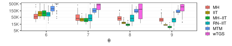
Figure 9: Box plots for the number of posterior calls needed to accurately approximate $\pi$ (see the main text) in Example 1 with $p=500$ and $p_{1}=20$. For each $\theta$, we repeat the simulation $50$ times. All samplers are forced to stop after $500$ thousand posterior calls. MH: uninformed MH; IIT: Algorithm 1; MH-IIT: Algorithm 2; RN-IIT Algorithm 3; MTM: the method of [11]; wTGS: the method of [49].

C.3 More details about the simulation study on Example 2

Details of the MCMC samplers.

Settings of MH, RN-IIT, MTM and wTGS are the same as in Example 1. MH-IIT-1 is the same as MH-IIT in Example 1. For MH-IIT-2, we still use $\rho(x)\equiv 0.025$ but change the balancing function to $h_{c}(r)$ with $c=2\theta$, where $h_{c}$ is defined by (9).

Remarks on $h_{c}$.

Equivalently, we can express $h_{c}$ by

$$h_{c}(r)=\left\{\begin{array}[]{cc}1,&\text{ if }x\geq e^{c},\\ re^{-c},&\text{ if }1\leq r<e^{c},\\ e^{-c},&\text{ if }e^{-c}<x<1,\\ r,&\text{ if }x\leq e^{-c}.\end{array}\right.$$

It is straightforward to check that $h_{c}$ is indeed a balancing function for any $c\geq 0$. When $c=0$, we get $h_{c}(r)=1\wedge r$. As $c\rightarrow\infty$, we get $e^{c}\,h_{c}(r)=1\vee r$. Hence, a larger $c$ implies more aggressive behavior of the corresponding informed proposal.

According to the definition of $\pi$ in Example 2, for any $x\in\mathcal{X}$ and $y\in\mathcal{N}_{x}$, we have $|\log\frac{\pi(y)}{\pi(x)}|\geq\theta$. Hence, for this particular example, using $c=0$, $c=\theta$, or any other value in $(0,\theta)$ do not make a difference. In particular, if $x_{1}=0$, according to the definition of $\pi$, we have

$$\frac{\pi(y)}{\pi(x)}=\left\{\begin{array}[]{cc}\mathrm{exp}(\theta)&\text{ if }y\in\mathcal{N}_{x},\lVert y\rVert_{1}=\lVert x\rVert_{1}+1,y_{1}=0,\\ \mathrm{exp}(2\theta(p-\lVert x\rVert_{1}))&\text{ if }y\in\mathcal{N}_{x},y_{1}=1.\end{array}\right.$$

Hence, using $h_{c}$ with $c>\theta$ encourages the sampler to add the first covariate to $x$ in this case. Of course, in practice, we usually do not have much knowledge about $\pi$ for tuning the parameter $c$. The primary purpose of this simulation study is to illustrate that for MH-IIT schemes, it is often desirable to use a balancing function more aggressive than the default one, $h(r)=1\wedge r$.

Complexity of MH-IIT schemes for $p=5$.

In Section 4, we introduced the metric $\mathrm{Comp}(h,\rho)$, defined in (11), for measuring the complexity of MH-IIT schemes, i.e., Algorithm 2. In Figure 10, we plot $\mathrm{Gap}(\mathsf{P}^{\mathrm{ct}}_{h})$ and $\mathrm{Comp}(h,\rho)$ for MH-IIT schems with balancing function $h_{c}$ in Example 2 with $p=5$. Optimal values of the spectral gap and complexity have already been reported in Table 1.

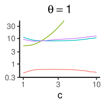
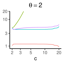
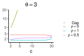
Figure 10: Complexity of MH-IIT schemes with balancing function $h_{c}$ in Example 2 with $p=5$. We consider three choices of $\rho$ and numerically calculate $\mathrm{Gap}(\mathsf{P}^{\mathrm{ct}}_{h})$ and $\mathrm{Comp}(h,\rho)$ for different choices of $c$. Gap (red line): spectral gap $\mathrm{Gap}(\mathsf{P}^{\mathrm{ct}}_{h})$, which is independent of $\rho$. $\rho=0$ (green line): $\mathrm{Comp}(h,\rho)$ with $\rho\equiv 0$ (uninformed MH). $\rho=1$ (blue line): $\mathrm{Comp}(h,\rho)$ with $\rho\equiv 1$ (naive IIT). $\rho=0.5$ (purple line): $\mathrm{Comp}(h,\rho)$ with $\rho\equiv 0.5$.

C.4 More details about the simulation study on Example 3

Details of the MCMC samplers.

The six samplers are the same as those investigated in Example 1. Regarding the parameter settings, the only difference is that we now use $m=40$ for RN-IIT, since $p=200$ in this example while $p=500$ in Example 1. Results for $p_{1}=20$ are given in Figure 11, from which we obtain essentially same findings for the three IIT methods.

Remarks on wTGS.

We note that, unlike in the the other two example, wTGS has very good performance in this bimodal setting. Indeed, Figure 11 shows that when $p_{1}=20$, wTGS has the best performance once $\theta$ becomes sufficiently large. We give an intuitive explanation here. Observe that a sampler can move from $x_{(1)}^{*}$ to $x_{(2)}^{*}$ by either removing the first covariate from $x_{(1)}^{*}$ or adding the second covariate to $x_{(1)}^{*}$. When $p_{1}\ll p$, it is much easier for the sampler to remove the right covariate than to add the right one. Compared to IIT methods, the informed proposal used by wTGS favors removing covariates from $x_{(1)}^{*}$ (the proposal scheme of wTGS was explained in Appendix C.2), which makes wTGS able to move between the two local modes more easily than IIT methods. Nevertheless, as we have shown in Section 3.2, wTGS seems to be inferior to the IIT methods for multimodal targets arising in realistic variable selection problems.

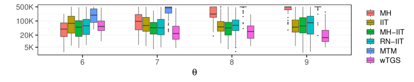
Figure 11: Box plot for the number of posterior calls (truncated at 500K) needed to accurately approximate $\pi$ in Example 3 with $p=200$ and $p_{1}=20$. Each box represents $50$ runs. MH: uninformed MH; IIT: Algorithm 1; MH-IIT: Algorithm 2; RN-IIT Algorithm 3; MTM: the method of [11]; wTGS: the method of [49].

C.5 More details about the variable selection simulation study

The nine MCMC samplers are set up as follows. MH, IIT, RN-IIT, MTM and wTGS are the same as in Example 1. In particular, the parameter $m$ in RN-IIT and the number of tries in MTM are set to $100$, and for IIT, RN-IIT and MTM, the balancing function is $h(r)=\sqrt{r}$. For the two MH-IIT methods, we fix $\rho=0.0025$. For MH-IIT-1, we use the conservative balancing function $h(r)=\min\{1,r\}$, and for MH-IIT-2, we use the balancing function $h$ defined in (9) with $c=8$. For HBS, we utilize the code provided in Zanella and Roberts [49], which considers a Hamming ball with radius 1 centered at the current model in each iteration. For LIT-MH, we use the parameter setting of the LIT-MH-2 algorithm presented in Zhou et al. [52].

Appendix D Supplements for the other simulation studies

D.1 More details about the simulation study in Section 5.3

Identifying six local modes.

We have checked that the signal size is sufficiently large so that the true model $\{1,2,3\}$ has a much larger posterior probability than others (except the other five local modes). To find the other equally good models, first observe that $\bm{L}_{2},\bm{L}_{3},\bm{L}_{4}$ are almost linearly dependent by construction (the normal error is almost negligible since the variance is only $1$% that of $\bm{L}_{2}$ or $\bm{L}_{3}$). Hence, $\{1,2,4\}$ or $\{1,3,4\}$ are both as good as the true model, and which one has a slightly larger posterior probability depends on which can happen to explain more variation in the noise part of $\bm{Y}$. However, $\{2,3,4\}$ is not comparable to the three models since it does not contain information about $\bm{L}_{1}$. Next, the construction of $\bm{L}_{5}$ guarantees that $\bm{L}_{1}+\bm{L}_{2}+\bm{L}_{3}$ is almost the same as $\bm{X}_{5}-\bm{X}_{6}-\bm{X}_{7}$, suggesting that $\{5,6,7\}$ may behave just like the true model. Since $\bm{L}_{6},\bm{L}_{7},\bm{L}_{8}$ are almost linearly dependent, models $\{5,6,8\}$ and $\{5,7,8\}$ should be as good as $\{5,6,7\}$.

We say these six models are local modes since their posterior probabilities cannot be increased by adding or removing one covariate (swap moves are not considered in this paper). Table 3 lists the un-normalized posterior probabilities of the six local modes for the data set we generate.

	$\{1,2,3\}$	$\{1,2,4\}$	$\{1,3,4)\}$	$\{5,6,7\}$	$\{5,6,8\}$	$\{5,7,8\}$
log-posterior	73.24	73.40	73.93	70.41	70.46	67.20

Table 3: Log posterior probabilities (un-normalized) of the six local modes in the example considered in Section 5.3.

Choosing $\psi_{j}$ and $\phi_{j}$.

The classical theory of simulated and parallel tempering suggests that we prefer to set $\psi_{j}$ to be the inverse normalizing constant of the distribution $\pi(\bm{\gamma})^{a_{j}}$, which unfortunately is almost impossible to estimate before sampling. Hence, we use the method of Geyer and Thompson [18] to dynamically update $\psi_{j}$. The main idea is that if the sampler is currently at temperature $1/a_{j}$, we can reduce the weight $\psi_{j}$ to encourage the sampler to move to other temperatures. Specifically, let $n_{0}$ and $s_{0}$ be two positive constants and initialize $\psi_{j}=1$ for every $j$. Suppose that in the $k$-th iteration the inverse temperature is given by $a_{j}$ with $j=j^{(k)}$. Then, we update $\psi_{j}$ by

$$\begin{split}\log\frac{1}{\psi_{j^{(k)}}}&\leftarrow\log\frac{1}{\psi_{j^{(k)}}}+\frac{s_{0}}{n_{0}+k},\\ \log\frac{1}{\psi_{j}}&\leftarrow\log\frac{1}{\psi_{j}}-\frac{s_{0}}{J(n_{0}+k)},\text{ for all }j\neq j^{(k)}.\end{split}$$

We fix $s_{0}=n_{0}=100$ throughout our simulation study.

The choice of $\{\phi_{j}\}_{j=0}^{J}$ can have a significant impact on the efficiency of the importance sampling estimators constructed using the samples and importance weights generated from Algorithm 5. This has been carefully studied in [19], and we recommend using their method. For simplicity, in this simulation study, we only look at the sample trajectory of Algorithm 5 (but not the weights), and thus the choice of $\{\phi_{j}\}_{j=0}^{J}$ is irrelevant.

Simulation results for $J=9$

Table 4 gives the results for 100 runs with $J=9$ (i.e., 10 temperatures). Each run consists of $5\times 10^{4}$ iterations. When $\Delta=1$, “Method 1” is still worse than the other two methods for choosing $\{h_{j}\}_{j=0}^{J}$ in that it gets stuck at one group of local modes in 12 runs. When $\Delta=2$, all three methods have similar performance. In particular, “Method 3” only gets stuck at one group of local modes in one run, but apparently it needs more iterations to identify all the six local modes.

		$\Delta=1$			$\Delta=2$
No. local modes	IIT	M1	M2	M3	M1	M2	M3
3	100	12	2	6	2	2	1
4	0	1	2	1	5	8	10
5	0	8	3	6	15	18	21
6	0	79	93	87	78	72	68

Table 4: The number of distinct local modes (max=6) that have been visited by Algorithm 5 with $J=9$ for the variable selection problem constructed in Section 5.3. IIT: Algorithm 1 without tempering. $\Delta$: the parameter used in the temperature ladder. M1/M2/M3: the three methods for choosing $\{h_{j}\}_{j=0}^{J}$ (see main text for details).

D.2 Pseudo-marginal methods for Example 2

Consider Example 2 again with $p=500$, $\pi(x)=\mathrm{exp}(-\theta\,\ell(x))/\mathfrak{C}_{\theta}$, where $\ell(x)$ and $\mathfrak{C}$ are given by (8). Instead of directly calculating $\pi$ (up to a normalizing constant), we assume that the parameter $\theta$ is unknown but we have an unbiased estimator $\hat{\theta}\sim N(\theta,\sigma^{2})$. Hence, the unbiased estimate of the un-normalized posterior probability can be calculated by

$$\hat{\pi}(x)\propto\mathrm{exp}\left\{-\hat{\theta}\,\ell(x)-\frac{\ell(x)^{2}\sigma^{2}}{2}\right\}.$$

We then run the simulation study using the same setting as in Section 3.1 and investigate how many posterior calls are needed in order to approximate $\pi$ accurately. That is, we define $F(x)=(\lVert x\rVert_{1}-1)\mathbbm{1}_{\{x_{1}=1\}}+p\mathbbm{1}_{\{x_{1}=0\}}$, initialize the sampler at some $x^{(0)}$ with the last 10 coordinates being $1$, and count the posterior calls needed to achieve $d(\pi,\hat{\pi}_{T};F)\leq 0.2$. Results for the standard pseudo-marginal uninformed MH algorithm and Algorithm 6 are shown in Figure 12. The advantage of the use of importance tempering is as significant as in Figure 2. When $\sigma$ is small, indicating a small variance of the posterior estimator, results are very similar to the simulation study in Section 3.1. But as $\sigma$ increases, both methods require more iterations to converge.

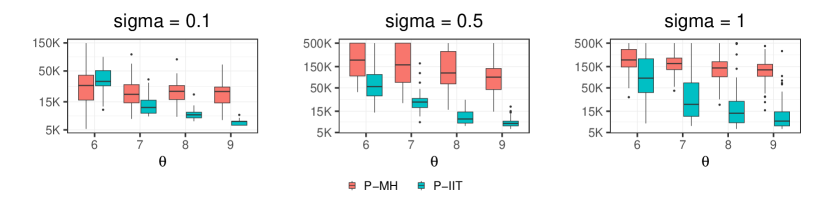
Figure 12: Box plot for the number of posterior calls (truncated at 500K) needed to accurately approximate $\pi$ in Example 2 with $p=500$. Each box represents $50$ runs. P-MH: pseudo-marginal uninformed MH; P-IIT: Algorithm 6 with $h(r)=\sqrt{r}$. A larger sigma indicates a larger variance of the posterior estimate.

D.3 On the toy example considered in Section 6.2

For the geometric distribution example in Section 6.2, we have state space $\mathcal{X}=\{1,2,\dots\}$ and $\mathcal{N}_{x}=\{x-1,x+1\}$ if $x\geq 2$ and $\mathcal{N}_{x}=\{2\}$ if $x=1$. One can still run Algorithm 6 to generate samples $x^{(1)},x^{(2)},\dots$, but the importance weights are biased.

Why Algorithm 6 is biased.

Denote the posterior estimate by $\hat{\pi}(x)=u\pi(x)$. As in Appendix B.4, we consider the joint space $(x,u,u_{-},u_{+})$ such that $\hat{\pi}(x)=u\pi(x)$, $\hat{\pi}(x-1)=u_{-}\pi(x-1)/$, $\hat{\pi}(x+1)=u_{+}\pi(x+1)$. (If $x=1$, we only need to consider the state variable $(x,u,u_{+})$.) The argument used in Appendix B.4 shows that the stationary distribution of Algorithm 6 is

$$\pi_{\mathrm{pm}}(x,u,u_{-},u_{+})\propto u\,\pi(x)Z_{h}(x,u,u_{-},u_{+})\mathsf{T}(x,u)\mathsf{T}(x-1,u_{-})\mathsf{T}(x+1,u_{+}),$$

where $\mathsf{T}(x,\cdot)$ denotes the distribution $(Kb^{x})^{-1}\mathrm{Binom}(K,b^{x})$.

The key difference from the proof in Appendix B.4 is that now we have $Z_{h}(x,u,u_{-},u_{+})=0$ if $u>0$ but $u_{-}=u_{+}=0$. (If $x=1$, then $Z_{h}(x,u,u_{+})=0$ whenever $u_{+}=0$.) Consequently, if we still define the target distribution $\pi(x,u,u_{-},u_{+})$ as in Appendix B.4, then $\pi_{\mathrm{pm}}$ will have a strictly smaller support than $\pi$ and thus the importance weights of Algorithm 6 are biased.

Unbiased importance weights.

We can define our target distribution by

$$\pi(x,u,u_{-},u_{+})=\left\{\begin{array}[]{cc}u\,\pi(x)\mathsf{T}(x,u)\mathsf{T}(x-1,u_{-})\mathsf{T}(x+1,u_{+})B(x)^{-1},&\text{ if }u_{-}\neq 0\text{ or }u_{+}\neq 0,\\ 0,&\text{ if }u_{-}=u_{+}=0,\end{array}\right.$$

where $B(x)$ is the probability that $u_{-},u_{+}$ are not both equal to zero, when $u_{-}\sim\mathsf{T}(x-1,\cdot)$ and $u_{+}\sim\mathsf{T}(x+1,\cdot)$. (If $x=1$, $B(x)$ is the probability that $u_{+}>0$.) One can calculate that

$$B(x)=\left\{\begin{array}[]{cc}1-(1-b^{x+1})^{K},&\text{ if }x=1,\\ 1-(1-b^{x-1})^{K}(1-b^{x+1})^{K},&\text{ if }x\geq 2\end{array}\right.$$

Clearly, $\pi(x,u,u_{-},u_{+})$ still has $\pi(x)$ as the marginal. The corrected importance weight is given by $[Z_{h}(x,u,u_{-},u_{+})B(x)]^{-1}$.

Should we correct for the bias?

The above discussion reveals that the importance weight of Algorithm 6 needs to be multiplied by a correction factor $1/B(x)$. However, observe that $1/B(x)\rightarrow\infty$ as $x\rightarrow\infty$, which can make the importance sampling estimates of P-IIT unstable. Indeed, we find in our simulation study that when the factor $1/B(x)$ is taken into account, the performance of P-IIT becomes quite similar to that of P-MH. If the factor $1/B(x)$ is not included, which means that we still use slightly biased importance weight estimates of Algorithm 6, we find that the performance of P-IIT is significantly improved, as shown in Figure 6 in the main text. Intuitively, if the P-MH sampler is at some large $x$ and $\tilde{U}_{x}$ happens to be large as well, the chain can get stuck at $x$ for a huge number of iterations since it is very difficult to get non-zero posterior estimates for the neighboring states $x-1$ and $x+1$ (recall that the success probability for the binomial distribution of $\tilde{U}_{x}$ decreases to $0$ exponentially fast in $x$). This causes P-MH to have unbounded asymptotic variance [28]. For P-IIT, we can force the chain to keep moving but need to estimate the holding time which is also unbounded. When we do not include $1/B(x)$ in the importance weight calculation, we are essentially using a biased but much more stable estimate for the holding time, and our simulation study confirms that this leads to much better MCMC estimates in practice.

D.4 More results for the simulation study in Section 7.2

Figure 13 shows the box plots analogous to the right panel of Figure 7, where we use the last $10\%$ of the samples or all samples to calculate the estimates of $M_{2,p}$. When last $10\%$ samples are used, the result is highly similar to that presented in Figure 7 (which uses last $50\%$ of the samples); one small difference is that the variance of the estimates of MTM methods have been slightly reduced. When all samples are used, only MT-IT with $h(r)=\sqrt{r}$ yields unbiased estimates, and the bias of the four MTM methods is very large.

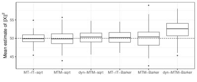
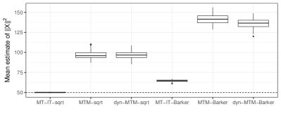
Figure 13: Box plots of the estimate of the mean of $\lVert x\rVert_{2}^{2}$ over 100 runs in the example considered in Section 7.2 with $p=50$. The theoretical value is given by $p=50$. Left: estimates are calculated by using the last 10% samples. Right: estimates are calculated by using all samples. MT-IT: Algorithm 7 with fixed proposal; MTM: MTM with fixed proposal [17]; dyn-MTM: adaptive MTM used in [17]; sqrt: $h(r)=\sqrt{r}$; Barker: $h(r)=r/(1+r)$.

Appendix E Supplements for the record linkage problem

E.1 Posterior distribution

Assume that all the $K$ covariates are categorical, and each has $L$ levels. Let $n_{\bm{M}}=\sum_{i=1}^{n_{1}}\mathbbm{1}\{M_{i}>0\}$ denote the number of matched pairs in $\bm{M}$. The target posterior distribution considered in Zanella [48] is given by

$$\pi(\bm{M},p_{\mathrm{match}},\lambda)\propto \;e^{-\lambda}\lambda^{n_{1}+n_{2}-n_{\bm{M}}}\left(\frac{1-p_{\mathrm{match}}}{2}\right)^{n_{1}+n_{2}-2n_{\bm{M}}}p_{\mathrm{match}}^{n_{\bm{M}}}$$

$$\times\prod_{k=1}^{K}\prod_{i\colon M_{i}>0}\left(\zeta(2-\zeta)+\frac{(1-\zeta)^{2}}{\theta_{ka_{ik}}}\mathbbm{1}\{a_{ik}=b_{M_{i}k}\}\right)$$

$$\times\mathbbm{1}\{0\leq p_{\mathrm{match}}\leq 1\}\mathbbm{1}\{n_{1}\wedge n_{2}\leq\lambda\leq n_{1}+n_{2}\},$$

where $\zeta$ and $\{\theta_{kl}\colon k=1,\dots,K,\,l=1,\dots,L\}$ are some parameters assumed to be known. In our study, we use $\zeta=0.001$ and estimate $\theta_{kl}$ (the frequency of the $l$-th category of the $k$-th covariate) using empirical frequencies. The unknown hyperparameter $\lambda$ gives the expected number of unique entities in $\bm{A}$ and $\bm{B}$, and $p_{\mathrm{match}}$ can be interpreted as the probability that an entity has duplicate records (see [48] for details). The following conditional distributions are used in the MCMC sampling:

$$\pi(\bm{M}\,|\,p_{\mathrm{match}},\lambda)\propto\; \prod_{i:M_{i}>0}\left\{\frac{4p_{\mathrm{match}}}{\lambda(1-p_{\mathrm{match}})^{2}}\prod_{k=1}^{K}\biggl{(}\zeta(2-\zeta)+\frac{(1-\zeta)^{2}}{\theta_{ka_{ik}}}\mathbbm{1}\{a_{ik}=b_{M_{i}k}\}\biggr{)}\right\},$$

$$p_{\mathrm{match}}\,|\,\bm{M},\lambda\sim\; \text{Beta}(n_{m}+1,n_{1}+n_{2}-2n_{\bm{M}}+1),$$

$$\lambda\,|\,\bm{M},p_{\mathrm{match}}\sim\; \text{Gamma}_{[n_{1}\wedge n_{2},n_{1}+n_{2}]}(n_{1}+n_{2}-n_{\bm{M}}+1,1),$$

where $\text{Gamma}_{c_{1},c_{2}}$ denotes the Gamma distribution truncated to $[c_{1},c_{2}]$. We refer readers to Zanella [48] for the details of the Bayesian modeling of the record linkage problem.

E.2 Neighborhood and local proposals for $M$

Fix an arbitrary $\bm{M}$ such that each record in one data set is matched with at most one record in the other data set. we construct a neighborhood $\mathcal{N}_{\bm{M}}=\{\bm{M}^{ij}\colon i=1,\dots,n_{1},\;j=1,\dots,n_{2}\}$ where $\bm{M}^{ij}$ is obtained from $\bm{M}$ by one of the following moves.

• Add move: If $M_{i}=0$ and $M_{j}^{-1}=0$, we set $M^{ij}_{i}=j$.

• Delete move: If $M_{i}=j$, we set $M^{ij}_{i}=0$.

• Single switch move (first type): If $M_{i}=0$ and $M_{j}^{-1}=i^{\prime}$ for some $i^{\prime}\neq i$, we set $M^{ij}_{i}=j$ and $M^{ij}_{i^{\prime}}=0$.

• Single switch move (second type): If $M_{i}=j^{\prime}$ for some $j^{\prime}\neq j$ and $M_{j}^{-1}=0$, we set $M^{ij}_{i}=j$.

• Double switch move: If $M_{i}=j^{\prime}$ for some $j^{\prime}\neq j$ and $M_{j}^{-1}=i^{\prime}$ for some $i^{\prime}\neq i$, we set $M^{ij}_{i}=j$ and $M^{ij}_{i^{\prime}}=j^{\prime}$.

It is not difficult to check that each pair $(i,j)$ yields a unique $\bm{M}^{ij}$, and thus $|\mathcal{N}_{\bm{M}}|=n_{1}n_{2}$.

E.3 More details about the samplers

We describe how each iteration of the three sampler is performed. We use $(\bm{M},p_{\mathrm{match}},\lambda)$ to denote the current state, and use $(\bm{M}^{\prime},p^{\prime}_{\mathrm{match}},\lambda^{\prime})$ to denote the next.

Uninformed MH.

This refers to the standard Metropolis-within-Gibbs sampler. Each iteration has two steps. First, we draw $(p_{\mathrm{match}}^{\prime},\lambda^{\prime})$ from the conditional posterior distribution (which is known) given $\bm{M}$. Second, we propose $\tilde{\bm{M}}$ by a uniform sampling from the neighborhood $\mathcal{N}_{\bm{M}}$ and accept it with probability $\min\{1,\pi(\tilde{\bm{M}}\,|\,p_{\mathrm{match}}^{\prime},\lambda^{\prime})/\pi(\bm{M}\,|\,p_{\mathrm{match}}^{\prime},\lambda^{\prime})\}$. Set $\bm{M}^{\prime}=\tilde{\bm{M}}$ if the proposal is accepted, and $\bm{M}^{\prime}=\bm{M}$ otherwise. Each iteration involves two posterior calls since we need to get both $\pi(\bm{M}\,|\,p_{\mathrm{match}}^{\prime},\lambda^{\prime})$ and $\pi(\tilde{\bm{M}}\,|\,p_{\mathrm{match}}^{\prime},\lambda^{\prime})$.

Informed MH.

This refers to the Metropolis-within-Gibbs sampler where $\bm{M}$ is updated by a locally balanced informed proposal. In each iteration, we first draw $(p_{\mathrm{match}}^{\prime},\lambda^{\prime})$ from the conditional distribution given $\bm{M}$. Next, we randomly select a subset of indices $\mathcal{I}\subset\{1,2,\dots,n_{1}\}$ and $\mathcal{J}\subset\{1,2,\dots,n_{2}\}$ and apply an informed proposal with balancing function $h(r)=\sqrt{r}$ to the neighborhood subset $\{\bm{M}^{ij}\colon i\in\mathcal{I},\,j\in\mathcal{J}\}\subset\mathcal{N}_{\bm{M}}$, where $\bm{M}^{ij}$ is as defined in the last section. This blocking strategy was used in [48] to reduce the computational cost of each informed MH update. Let $\tilde{\bm{M}}$ denote the proposed value. To calculate the acceptance probability, we need to evaluate both $\pi(\bm{M}^{ij}\,|\,p_{\mathrm{match}}^{\prime},\lambda^{\prime})$ and $\pi(\tilde{\bm{M}}^{ij}\,|\,p_{\mathrm{match}}^{\prime},\lambda^{\prime})$ for each $i\in\mathcal{I}$ and $j\in\mathcal{J}$. In our implementation, we set $|\mathcal{I}|=|\mathcal{J}|=10$, and thus each iteration involves $2|\mathcal{I}||\mathcal{J}|+1=201$ posterior calls.

MT-IT.

As described in the main text, we apply Algorithm 7 with $\mathsf{Q}$ being a mixture proposal scheme. More precisely, letting $x=(\bm{M},p_{\mathrm{match}},\lambda)$, we propose $m$ candidate moves, denoted by $(x_{1},\dots,x_{m})$, such that each $x_{i}$ is proposed independently as follows. With probability $\delta$, we set $x_{i}=(\bm{M},\tilde{p}_{\mathrm{match}},\tilde{\lambda})$ where $(\tilde{p}_{\mathrm{match}},\tilde{\lambda})$ is drawn from the conditional distribution given $\bm{M}$. With probability $1-\delta$, we set $x_{i}=(\tilde{\bm{M}},p_{\mathrm{match}},\lambda)$ where $\tilde{\bm{M}}$ is sampled from $\mathcal{N}_{\bm{M}}$ uniformly at random. We set $\delta=0.99$ and $m=100$ so that the MT-IT has a similar dynamics to the informed MH. Each iteration of MT-IT involves $m=100$ posterior calls.

E.4 Results for other regions

We find that the performance of the three samplers mostly depends on the sample size $n_{1},n_{2}$. Figure 14 displays the results for three other representative regions. Region 18 has a relatively small sample size (similar to region 4 shown in the main text), $n_{1}=294$ and $n_{2}=292$. Region 20 has a moderate sample size, $n_{1}=637$ and $n_{2}=641$. Region 1 has a large sample size, $n_{1}=1285$ and $n_{2}=1121$. For both region 20 and region 1, the three samplers are not able to converge after $8\times 10^{5}$ posterior calls, but we still observe that the log-posterior curve of MT-IT increases much faster than that of the other two samplers. Interestingly, it can be seen that the number of matched pairs does not necessarily reflect the efficiency of the sampler, especially when the sampler has not converged (this statistic was also used in [48]). Compared to MH algorithms, MT-IT is more likely to visit some $\bm{M}$ with fewer matched pairs but higher posterior probability in the early stage of the sampling.

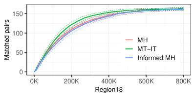
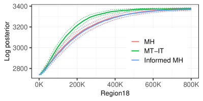
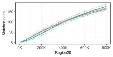
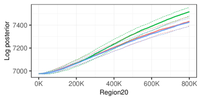
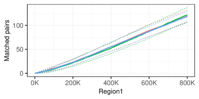
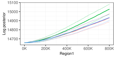
Figure 14: Results for the record linkage analysis of regions 1, 18 and 20 in the R package italy. The solid colored lines represent the average values obtained from 50 runs, and dashed lines indicate $\pm 1$ standard deviation. MH: Metropolis-within-Gibbs sampler with uninformed MH updates; informed MH: Metropolis-within-Gibbs sampler with informed MH updates; MT-IT: Algorithm 7.

References

- Aldous and Fill [2002] David Aldous and Jim Fill. Reversible Markov chains and random walks on graphs, 2002. URL https://www.stat.berkeley.edu/~aldous/RWG/book.html.
- Andral et al. [2022] Charly Andral, Randal Douc, Hugo Marival, and Christian P Robert. The importance Markov chain. arXiv preprint arXiv:2207.08271, 2022.
- Andrieu and Roberts [2009] Christophe Andrieu and Gareth O Roberts. The pseudo-marginal approach for efficient Monte Carlo computations. The Annals of Statistics, 37(2):697–725, 2009.
- Andrieu and Vihola [2015] Christophe Andrieu and Matti Vihola. Convergence properties of pseudo-marginal Markov chain Monte Carlo algorithms. Annals of Applied Probability, 25(2):1030–1077, 2015.
- Atchadé and Perron [2005] Yves F Atchadé and François Perron. Improving on the independent Metropolis–Hastings algorithm. Statistica Sinica, 15(1):3–18, 2005.
- Baldassi [2017] Carlo Baldassi. A method to reduce the rejection rate in Monte Carlo Markov chains. Journal of Statistical Mechanics: Theory and Experiment, 2017(3):033301, 2017.
- Barker [1965] Anthony Alfred Barker. Monte Carlo calculations of the radial distribution functions for a proton-electron plasma. Australian Journal of Physics, 18(2):119–134, 1965.
- Bornn et al. [2017] Luke Bornn, Natesh S Pillai, Aaron Smith, and Dawn Woodard. The use of a single pseudo-sample in approximate Bayesian computation. Statistics and Computing, 27:583–590, 2017.
- Brémaud [2013] Pierre Brémaud. Markov chains: Gibbs fields, Monte Carlo simulation, and queues, volume 31. Springer Science & Business Media, 2013.
- Casella and Robert [1996] George Casella and Christian P Robert. Rao-Blackwellisation of sampling schemes. Biometrika, 83(1):81–94, 1996.
- Chang et al. [2022] Hyunwoong Chang, Changwoo J Lee, Zhao Tang Luo, Huiyan Sang, and Quan Zhou. Rapidly mixing multiple-try Metropolis algorithms for model selection problems. In Advances in Neural Information Processing Systems, 2022.
- Dall and Sibani [2001] Jesper Dall and Paolo Sibani. Faster Monte Carlo simulations at low temperatures. The waiting time method. Computer physics communications, 141(2):260–267, 2001.
- Deligiannidis and Lee [2018] George Deligiannidis and Anthony Lee. Which ergodic averages have finite asymptotic variance? Annals of Applied Probability, 28(4):2309–2334, 2018.
- Douc and Robert [2011] Randal Douc and Christian P Robert. A vanilla Rao–Blackwellization of Metropolis–Hastings algorithms. The Annals of Statistics, 39(1):261–277, 2011.
- Douc et al. [2018] Randal Douc, Eric Moulines, Pierre Priouret, and Philippe Soulier. Markov chains. Springer, 2018.
- Franks and Vihola [2020] Jordan Franks and Matti Vihola. Importance sampling correction versus standard averages of reversible MCMCs in terms of the asymptotic variance. Stochastic Processes and their Applications, 130(10):6157–6183, 2020.
- Gagnon et al. [2022] Philippe Gagnon, Florian Maire, and Giacomo Zanella. Improving multiple-try Metropolis with local balancing. arXiv preprint arXiv:2211.11613, 2022.
- Geyer and Thompson [1995] Charles J Geyer and Elizabeth A Thompson. Annealing Markov chain Monte Carlo with applications to ancestral inference. Journal of the American Statistical Association, 90(431):909–920, 1995.
- Gramacy et al. [2010] Robert Gramacy, Richard Samworth, and Ruth King. Importance tempering. Statistics and Computing, 20(1):1–7, 2010.
- Griffin et al. [2021] Jim E Griffin, Krzysztof G Łatuszyński, and Mark FJ Steel. In search of lost mixing time: adaptive Markov chain Monte Carlo schemes for Bayesian variable selection with very large p. Biometrika, 108(1):53–69, 2021.
- Guan and Stephens [2011] Yongtao Guan and Matthew Stephens. Bayesian variable selection regression for genome-wide association studies and other large-scale problems. The Annals of Applied Statistics, 5(3):1780–1815, 2011.
- Hamze and Freitas [2007] Firas Hamze and Nando de Freitas. Large-flip importance sampling. In Proceedings of the Twenty-Third Conference on Uncertainty in Artificial Intelligence, pages 167–174, 2007.
- Hastings [1970] W Keith Hastings. Monte Carlo sampling methods using Markov chains and their applications. Biometrika, 57(1):97–109, 04 1970.
- Iliopoulos and Malefaki [2013] George Iliopoulos and Sonia Malefaki. Variance reduction of estimators arising from Metropolis–Hastings algorithms. Statistics and Computing, 23:577–587, 2013.
- Jacob et al. [2011] Pierre Jacob, Christian P Robert, and Murray H Smith. Using parallel computation to improve independent Metropolis–Hastings based estimation. Journal of Computational and Graphical Statistics, 20(3):616–635, 2011.
- Jennison [1993] Christopher Jennison. Discussion on the meeting on the Gibbs sampler and other Markov chain Monte Carlo methods. Journal of the Royal Statistical Society, Series B (Statistical Methodology), 55:54–56, 1993.
- Laddha et al. [2020] Aditi Laddha, Yin Tat Lee, and Santosh Vempala. Strong self-concordance and sampling. In Proceedings of the 52nd annual ACM SIGACT symposium on theory of computing, pages 1212–1222, 2020.
- Lee and Łatuszyński [2014] Anthony Lee and Krzysztof Łatuszyński. Variance bounding and geometric ergodicity of Markov chain Monte Carlo kernels for approximate Bayesian computation. Biometrika, 101(3):655–671, 2014.
- Lee et al. [2010] Anthony Lee, Christopher Yau, Michael B Giles, Arnaud Doucet, and Christopher C Holmes. On the utility of graphics cards to perform massively parallel simulation of advanced Monte Carlo methods. Journal of Computational and Graphical Statistics, 19(4):769–789, 2010.
- Liang [2002] Faming Liang. Dynamically weighted importance sampling in Monte Carlo computation. Journal of the American Statistical Association, 97(459):807–821, 2002.
- Liu et al. [2000] Jun S Liu, Faming Liang, and Wing Hung Wong. The multiple-try method and local optimization in Metropolis sampling. Journal of the American Statistical Association, 95(449):121–134, 2000.
- Liu et al. [2001] Jun S Liu, Faming Liang, and Wing Hung Wong. A theory for dynamic weighting in Monte Carlo computation. Journal of the American Statistical Association, 96(454):561–573, 2001.
- Livingstone and Zanella [2022] Samuel Livingstone and Giacomo Zanella. The Barker proposal: Combining robustness and efficiency in gradient-based mcmc. Journal of the Royal Statistical Society. Series B, Statistical Methodology, 84(2):496, 2022.
- Marin et al. [2012] Jean-Michel Marin, Pierre Pudlo, Christian P Robert, and Robin J Ryder. Approximate Bayesian computational methods. Statistics and computing, 22(6):1167–1180, 2012.
- Murray et al. [2006] Iain Murray, Zoubin Ghahramani, and David JC MacKay. MCMC for doubly-intractable distributions. In Proceedings of the Twenty-Second Conference on Uncertainty in Artificial Intelligence, pages 359–366, 2006.
- Neal [2001] Radford M Neal. Annealed importance sampling. Statistics and computing, 11(2):125–139, 2001.
- Peskun [1973] Peter H Peskun. Optimum Monte-Carlo sampling using Markov chains. Biometrika, 60(3):607–612, 1973.
- Power and Goldman [2019] Samuel Power and Jacob Vorstrup Goldman. Accelerated sampling on discrete spaces with non-reversible Markov processes. arXiv preprint arXiv:1912.04681, 2019.
- Rudolf and Sprungk [2020] Daniel Rudolf and Björn Sprungk. On a Metropolis–Hastings importance sampling estimator. Electronic Journal of Statistics, 14(1):857–889, 2020.
- Sahu and Zhigljavsky [2003] Sujit K Sahu and Anatoly A Zhigljavsky. Self-regenerative Markov chain Monte Carlo with adaptation. Bernoulli, 9(3):395–422, 2003.
- Schuster and Klebanov [2020] Ingmar Schuster and Ilja Klebanov. Markov chain importance sampling — a highly efficient estimator for MCMC. Journal of Computational and Graphical Statistics, pages 1–9, 2020.
- Sherlock et al. [2017] Chris Sherlock, Alexandre H Thiery, and Anthony Lee. Pseudo-marginal Metropolis–Hastings sampling using averages of unbiased estimators. Biometrika, 104(3):727–734, 2017.
- Tan et al. [2015] Aixin Tan, Hani Doss, and James P Hobert. Honest importance sampling with multiple Markov chains. Journal of Computational and Graphical Statistics, 24(3):792–826, 2015.
- Titsias and Yau [2017] Michalis K Titsias and Christopher Yau. The Hamming ball sampler. Journal of the American Statistical Association, 112(520):1598–1611, 2017.
- Vihola et al. [2020] Matti Vihola, Jouni Helske, and Jordan Franks. Importance sampling type estimators based on approximate marginal Markov chain Monte Carlo. Scandinavian Journal of Statistics, 47(4):1339–1376, 2020.
- Yang and Liu [2021] Xiaodong Yang and Jun S Liu. Convergence rate of multiple-try Metropolis independent sampler. arXiv preprint arXiv:2111.15084, 2021.
- Yang et al. [2016] Yun Yang, Martin J Wainwright, and Michael I Jordan. On the computational complexity of high-dimensional Bayesian variable selection. The Annals of Statistics, 44(6):2497–2532, 2016.
- Zanella [2020] Giacomo Zanella. Informed proposals for local MCMC in discrete spaces. Journal of the American Statistical Association, 115(530):852–865, 2020.
- Zanella and Roberts [2019] Giacomo Zanella and Gareth Roberts. Scalable importance tempering and Bayesian variable selection. Journal of the Royal Statistical Society Series B, 81(3):489–517, 2019.
- Zhou and Guan [2019] Quan Zhou and Yongtao Guan. Fast model-fitting of Bayesian variable selection regression using the iterative complex factorization algorithm. Bayesian Analysis, 14(2):573, 2019.
- Zhou and Smith [2022] Quan Zhou and Aaron Smith. Rapid convergence of informed importance tempering. In International Conference on Artificial Intelligence and Statistics, pages 10939–10965. PMLR, 2022.
- Zhou et al. [2022] Quan Zhou, Jun Yang, Dootika Vats, Gareth O Roberts, and Jeffrey S Rosenthal. Dimension-free mixing for high-dimensional Bayesian variable selection. Journal of the Royal Statistical Society: Series B (Statistical Methodology), to appear, 2022. doi: 10.1111/rssb.12546.