Twisted curve geometry underlying topological invariants

Abstract:

Topological invariants such as winding numbers and linking numbers appear as charges of topological solitons in diverse nonlinear physical systems described by a unit vector field defined on two and three dimensional manifolds. While the Gauss-Bonnet theorem shows that the Euler characteristic (a topological invariant) can be written as the integral of the Gaussian curvature (an intrinsic geometric quantity), the intriguing question of whether winding and linking numbers can also be expressed as integrals of some other kinds of intrinsic geometric quantities has not been addressed in the literature. In this paper we provide the answer by showing that for the winding number in two dimensions, these geometric quantities involve torsions of the two evolving space curves describing the manifold. On the other hand, in three dimensions we find that in addition to torsions, intrinsic twists of the space curves are necessary to obtain a nontrivial winding number and linking number. They arise from the hitherto unknown connections that we establish between these topological invariants and the corresponding appropriately normalized global space curve anholonomies (i.e., geometric phases) that can be associated with the unit vector fields on the respective manifolds. An application of our results to a 3D Heisenberg ferromagnetic model supporting a topological soliton is also presented.

1 Introduction

It is by now well recognized [1] that both geometry [2] and topology [3] of differentiable manifolds play an important role in a variety of fields such as condensed matter physics, high energy physics, fluid dynamics, biophysics, cosmology, etc. Topological invariants are quantities that take on discrete values (usually normalized to integers) that do not change under a continuous deformation of the manifold. Over the past couple of decades, the study of topological invariants such as winding numbers and linking numbers has become very valuable in the understanding of various phenomena in diverse fields of physics, including transitions between phases with different topological properties.

1.1 Gauss-Bonnet relationship

The well known Gauss-Bonnet theorem [2] leads to the result that the integral of the Gaussian curvature $K$ over the area of a compact two-dimensional manifold $M$ without a boundary is a topological invariant $\chi=2(1-g)$, called the Euler characteristic, where $g$ denotes the genus. It can be written as

$$\chi=\frac{1}{2\pi}\int_{M}K\,dA.$$ (1)

In the above, the Gaussian curvature $K$ is the product of the maximum and minimum curvatures on the surface at a point, given by $K=(R_{1}R_{2})^{-1}$, where $R_{1}$ and $R_{2}$ are the two corresponding radii of curvatures. However, $K$ can also be expressed entirely in terms of the metric, i.e., the coefficients of the first fundamental form of the 2D surface, and its partial derivatives [2]. It is therefore an intrinsic geometric quantity inherent in the manifold, independent of how it is embedded in space.

The Gauss-Bonnet relationship (1) shows that the Euler characteristic $\chi$ (a topological invariant) can be written as the integral of the Gaussian curvature $K$, an intrinsic geometric quantity. It is insightful to ask whether other topological invariants such as winding and linking numbers can also be similarly written as integrals of certain intrinsic geometric quantities. This provides a motivation for our paper. We will show that the answer is in the affirmative. Interestingly, in our quest for how to answer this question, we are led to several other new results that give us a deeper understanding of the geometry underlying topological invariants. We have listed these in Sec. 3, the concluding section of this paper.

1.2 Topological invariants (winding number and linking number)

To investigate whether the integrands appearing in winding and linking number expressions can be obtained in terms of some other kinds of intrinsic geometric quantities, we first scrutinize the known integral expressions for the 2D, 3D winding and linking numbers $W_{2}$, $W_{3}$ and $H$. These are given below in Eqs. (3), (8) and (38), respectively. As is obvious, their integrands typically involve angle variables, which are clearly not intrinsic geometric quantities. Further, to understand the physical relevance of our work, it is instructive to begin with examples of physical systems where topology plays an important role.

Topological invariants associated with a $3$-component unit vector field given by ${\bf t}({\bf r})$, with ${\bf r}$ representing physical space variables of the model considered, are of current interest and appear in a variety of physical systems. As examples we have the spin vector field in the continuum version of the classical Heisenberg model with various types of interactions between spins in magnetism [4, 5] and the vector field appearing in the nonlinear sigma model and its variants in high energy physics [6, 7]. It is noteworthy that these models are generically nonlinear, and (under appropriate conditions) support soliton solutions for the vector field [8]. These are localized, particle-like field configurations. (Baby) skyrmions and hopfions are well known examples of topological solitons [9, 10] in two and three dimensions, respectively. Topological invariants are physically interpreted as topological charges of such solitons.

The tip of the unit vector ${\bf t}$ lies on the two-sphere $S^{2}$. Consider a physical system with a homogeneous boundary condition ${\bf t}({\bf r})\rightarrow{\bf t}_{\infty}$, as ${\bf r}\rightarrow\infty$, where ${\bf t}_{\infty}$ is a constant vector. Under these conditions, the physical spaces $R^{1},R^{2}$ and $R^{3}$ can be compactified to $S^{1},S^{2}$ and $S^{3}$, respectively. Hence the unit vector field configurations represent maps from the (compactified) physical space to target space, given by ${\bf t}(x):S^{1}\rightarrow S^{2}$, ${\bf t}(x,y):S^{2}\rightarrow S^{2}$, and ${\bf t}(x,y,z):S^{3}\rightarrow S^{2}$, respectively. In addition, we note that using a normalized spinor representation [10], the target space $S^{2}$ can be written in terms of variables in $S^{3}$, resulting in the map ${\bf T}(x,y,z):S^{3}\rightarrow S^{3}$.

Among the above, the topological invariant of $S^{1}\rightarrow S^{2}$ is well known to be zero. The maps $S^{2}\rightarrow S^{2}$ and $S^{3}\rightarrow S^{3}$ are classified by integer topological invariants called winding numbers, denoted in this paper by $W_{2}$ and $W_{3}$, respectively. The former (respectively the latter) counts the number of times a sphere $S^{2}$ (respectively $S^{3}$) wraps around another such sphere. It is well known that the topological solitons associated with these maps are baby skyrmions (respectively skyrmions). In contrast, the map $S^{3}\rightarrow S^{2}$ involves manifolds with unequal dimensions. It is classified by an integer topological invariant $H$ known as the Hopf invariant. The corresponding topological solitons are called hopfions. It can be shown that $H$ also denotes the linking number of two closed space curves in $S^{3}$, which are preimages of any two distinct points on the target space $S^{2}$ [3].

Using spherical polar coordinates, with polar angle $\Theta$ and azimuthal angle $\Phi$, a 3-component unit vector field ${\bf t}$ representing $S^{2}$ is given by

$${\bf t}=\big{(}\sin\Theta\,\cos\Phi,\,\,\sin\Theta\,\sin\Phi,\,\,\cos\Theta\big{)}\,,$$ (2)

where $0\leq\Theta\leq\pi$ and $0\leq\Phi\leq 2\pi$.

The winding number $W_{2}$ in two dimensions is given by [8] the following integral over the 2D physical manifold described by $y$ and $z$ (say)

$$W_{2}=\frac{1}{4\pi}\int\int\sin\Theta\,\left[\Theta_{y}\Phi_{z}-\Theta_{z}\Phi_{y}\right]\,\,dy\,\,dz\,,$$ (3)

where the subscripts $y$ and $z$ on angles $\Theta$ and $\Phi$ denote partial derivatives with respect to these variables.

Next, we use the following Hopf coordinate representation [10] to describe a 4-component unit vector field ${\bf T}$ representing $S^{3}$

$${\bf T}=(x_{1},x_{2},x_{3},x_{4})$$ (4)

with

$$x_{1}=\cos\Theta/2\,\cos{\xi_{1}};\,\,x_{2}=\cos\Theta/2\,\sin{\xi_{1}};\,\,x_{3}=\sin\Theta/2\,\cos{\xi_{2}};\,\,x_{4}=\sin\Theta/2\,\sin{\xi_{2}},$$ (5)

where $0\leq\Theta\leq\pi$, $0\leq\xi_{1}\leq 2\pi$ and $0\leq\xi_{2}\leq 2\pi$. In Eq. (5), we find it convenient to set

$$\xi_{1}=(\tilde{\Psi}-\frac{\Phi}{2})\,\,;\,\,\xi_{2}=(\tilde{\Psi}+\frac{\Phi}{2}),$$ (6)

giving

$$\Phi=(\xi_{2}-\xi_{1})\,\,;\,\,\tilde{\Psi}=(\xi_{2}+\xi_{1})/2\,.$$ (7)

Thus $0\leq\Phi\leq 2\pi$, and $\tilde{\Psi}$ represents the third angle needed in addition to $(\Theta,\Phi)$ to define $S^{3}$. Further, $0\leq\tilde{\Psi}\leq 2\pi$.

The winding number $W_{3}$ in three dimensions is given by [11] the following integral over the 3D physical manifold

$$W_{3}=\frac{1}{8\pi^{2}}\int\int\int\sin\Theta\left\{[\Theta_{y}\Phi_{z}-\Theta_{z}\Phi_{y}]\,\,\tilde{\Psi}_{x}+[\Theta_{z}\Phi_{x}-\Theta_{x}\Phi_{z}]\,\,\tilde{\Psi}_{y}+[\Theta_{x}\Phi_{y}-\Theta_{y}\Phi_{x}]\,\,\tilde{\Psi}_{z}\right\}\,dx\,dy\,dz,$$ (8)

where the subscripts $x$, $y$ and $z$ on $\Theta$, $\Phi$ and $\tilde{\Psi}$ stand for partial derivatives with respect to these variables.

The integral expression for the linking number $H$ (Hopf invariant) characterizing the map $S^{3}\rightarrow S^{2}$ is more complicated than that of $W_{2}$ and $W_{3}$. First derived by Whitehead [12], it is given in Eq. (38) below, followed by a brief discussion of how it is computed.

It is important to note from Eqs. (3) and (8) that the integrands of the usual expressions for the winding numbers $W_{2}$ and $W_{3}$ are given explicitly in terms of $\Theta$ and the partial derivatives of all the angle coordinates of ${\bf t}$ and ${\bf T}$, respectively. However, it is not at all obvious that these integrands can be expressed in terms of geometric quantities. Needless to say, the same holds true for the linking number $H$ given in Eq. (38), whose integrand is not even given directly in terms of angle coordinates.

In the following sections, we will present an approach which shows that the integrands of the topological invariants $W_{2}$, $W_{3}$ and $H$ [given in Eqs. (3), (8) and (38), respectively] can indeed be expressed in terms of geometric quantities that define a space curve. We will derive these quantities explicitly, and provide their geometrical and physical interpretations.

1.3 Methodology: Anholonomy

The approach that we adopt to find the geometry underlying winding and linking numbers involves the concept of anholonomy. Anholonomy is a geometric phenomenon that arises if a quantity fails to recover its original value, when the parameters on which it depends are varied around a closed path in parameter space, and return to their original values. The concept of parallel transport, anholonomy and the associated geometric phase was first introduced by Berry in the quantum context [13]. However, as pointed out by Berry in [14], there is a direct correspondence between the anholonomy of a classical vector and that of a quantum state. Hence in the present paper which deals with classical anholonomy, we will use the quantum terminology such as Berry connection, Berry phase, Berry curvature, etc., for their classical analogs as well.

Our methodology is summarized as follows: We map the 3-component unit vector field ${\bf t}$ to the tangent of a space curve. We define a generalized Frenet-Serret frame for the space curve [2], where the plane composed of the normal and binormal vectors of the frame is rotated (i.e., twisted) around the tangent to the curve, by an arbitrary angle. We invoke the concept of parallel transport and find the associated anholonomy density (i.e., Berry connection) [13, 14] of the space curve depicting a 1D manifold. We then describe the 2D and 3D manifolds in terms of appropriate evolving space curves and find the associated global anholonomies. This leads to new relationships between winding and linking numbers and the corresponding (appropriately normalized) global anholonomies associated with the unit vector fields on the respective manifolds. These hitherto unknown connections help us to demonstrate that these topological invariants can be expressed as integrals involving certain geometric quantities appearing in the intrinsic description of a space curve. These will be found explicitly and interpreted physically in the next section.

2 Determination of topological invariants as integrals involving geometric quantities of a space curve

To set the stage for higher dimensions, it is instructive to begin with a one-dimensional manifold.

2.1 One-dimensional manifold

The following important observation is in order. As explained in Sec. 1.2, our starting point is a (given) 3-component unit vector ${\bf t}$. Let us associate ${\bf t}$ with the tangent of a three-dimensional space curve ${\bf R}(x)$ parametrized by $x$, such that ${\bf t}(x)=d{\bf R}(x)/dx$. Since ${\bf t}$ is a unit vector, this in turn implies that the arc length of the space curve, which is defined [2] by $s=\int|d{\bf R}(x)/dx|\,dx$ yields $x$. In other words, the arc length variable $s$ of the space curve gets directly identified with the physical coordinate variable $x$.

The usual Frenet-Serret equations for the orthogonal unit vector triad $({\bf t},{\bf n},{\bf b})$ defined on a space curve with arc length $x$ are given by [2]

$${\bf t}_{x}=k_{1}{\bf n}\,;~{}~{}{\bf n}_{x}=-k_{1}{\bf t}+\tau_{1}{\bf b}\,;~{}~{}{\bf b}_{x}=-\tau_{1}{\bf n}\,.$$ (9)

In Eq. (9), the subscript $x$ on the various vectors denotes derivative with respect to $x$. The principal normal vector ${\bf n}$ is defined to be along ${\bf t}_{x}$. The binormal vector is given by ${\bf b}={\bf t}\times{\bf n}$. Further, $k_{1}$ is the curvature, which measures the departure of a curve from a straight line, while $\tau_{1}$ is the torsion. It is a measure of the nonplanarity of the curve, i.e., the degree to which the curve twists out of a plane. As is well known [2], curvature $k=k_{1}(x)$ and torsion $\tau=\tau_{1}(x)$ are the intrinsic equations of the space curve.

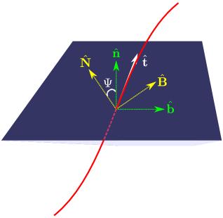
Figure 1: A space curve characterized by the unit triad $(\hat{\bf t},\hat{\bf n},\hat{\bf b})$ representing the tangent, normal and binormal to the curve. More generally, the curve can be represented by a rotated triad $(\hat{\bf t},\hat{\bf N},\hat{\bf B})$, with the angle of rotation of the $(\hat{\bf n},\hat{\bf b})$ plane around $\hat{\bf t}$ given by $\Psi$.

Clearly, one has the freedom to choose new unit vectors $({\bf N},{\bf B})$ perpendicular to ${\bf t}$ (Fig. 1), by rotating [15] the Frenet pair $({\bf n},{\bf b})$ around the tangent by an angle $\Psi$, with $0\leq\Psi\leq 2\pi$. This leads to

$${\bf N}={\bf n}\cos\Psi+{\bf b}\sin\Psi;\,\,\,~{}{\bf B}={\bf t}\times{\bf N}=-{\bf n}\sin\Psi+{\bf b}\cos\Psi.$$ (10)

Here, $\Psi$ can be physically interpreted as the local intrinsic twist of the $({\bf N},{\bf B})$ plane around the (tangential) axis of the space curve. This inherent freedom in the choice of $\Psi$ can also be regarded as a gauge freedom. As we will demonstrate, $\Psi$ plays a crucial role in unraveling the underlying geometry of certain topological invariants.

After a straightforward calculation using Eq. (10), the usual Frenet-Serret equations given in Eq. (9) can be written in terms of the rotated orthogonal unit triad $({\bf t},{\bf N},{\bf B})$ (see Fig. 1) as:

$${\bf t}_{x}=(k_{1}\cos\Psi){\bf N}-(k_{1}\sin\Psi){\bf B}\,,~{}~{}~{}{\bf N}_{x}=-(k_{1}\cos\Psi){\bf t}+\tau_{T,1}{\bf B}\,,~{}~{}~{}{\bf B}_{x}=(k_{1}\sin\Psi){\bf t}-\tau_{T,1}{\bf N}\,.$$ (11)

(For notational convenience, the subscripts $1$, $2$ and $3$ for the curve parameters $k$, $\tau$ and $\tau_{T}$ will be used to indicate that they correspond to a space curve parametrized by $x$, $y$ and $z$, respectively.)

In Eq. (11), the curvature $k_{1}=|\mathbf{t}_{x}|$, and $\tau_{T,1}$ is given by

$$\tau_{T,1}=\tau_{1}+\Psi_{x}\,,$$ (12)

where $\tau_{1}$ is the torsion that appears in the usual unrotated Frenet-Serret equations (9) and $\Psi_{x}$ denotes derivative of $\Psi$ with respect to $x$. As is well known [2], $\tau_{1}$ is given by

$$\tau_{1}=\mathbf{t}~{}\cdot~{}(\mathbf{t}_{x}~{}\times~{}\mathbf{t}_{xx})~{}/~{}k_{1}^{2}.$$ (13)

Adopting the nomenclature used by Moffatt and Ricca [15] in fluid dynamics, we refer to $\tau_{T,1}$ given in Eq. (12) as the total twist density of a space curve with arc length $x$. This is because $(1/2\pi)\int\tau_{T,1}dx$ has been called the ‘total twist number’ ($Tw$) of a thin ribbon constructed from the space curve using a standard procedure [16, 17]. We call the term $\Psi_{x}$ appearing in Eq. (12) as the intrinsic twist density, since its integral

$$(1/2\pi)\int\,\,\Psi_{x}\,\,dx=\,\mathcal{N}$$ (14)

is called the twist number. On integrating Eq. (12), we find that the total twist number is the sum of the total torsion and the twist number, as was defined in [15].

Returning to Eqs. (11), we note that the three equations for the triad $({\bf t},{\bf N},{\bf B})$ can be combined to give ${\bf G}_{x}=\boldsymbol{\xi}\times{\bf G}$, where ${\bf G}$ stands for ${\bf t},{\bf N}$ or ${\bf B}$. In the above, the Darboux vector [2] $\boldsymbol{\xi}$ that denotes the angular velocity of the rotation of the triad as one moves along the curve is given by

$$\boldsymbol{\xi}=\tau_{T,1}\,\,{\bf t}+(k_{1}\sin\Psi)\,\,{\bf N}+\,(k_{1}\cos\Psi)\,\,{\bf B}\,.$$ (15)

A non-rotating plane can be defined by using the usual parallel transport [18, 19] of the tangent vector ${\bf t}$ along the space curve in such a way that as $x$ changes to $(x+dx)$, the $({\bf N},{\bf B})$ plane gets rotated by an infinitesimal angle $\tau_{T,1}\,dx$ with respect to a non-rotating plane. This signifies an associated anholonomy density [13] (with angle per unit length as dimension) for the 1D manifold we are considering. It is the classical analog of Berry connection, which we denote by $V_{1}$. It is given by

$$V_{1}=\tau_{T,1}.$$ (16)

Eq. (12) shows that $V_{1}$ is a gauge dependent quantity, since the rotation angle $\Psi(x)$ can be arbitrary.

It is instructive to express $\tau_{1}$ in terms of spherical polar coordinates of ${\bf t}$, by substituting Eq. (2) in Eq. (13). Using $k_{1}=|\mathbf{t}_{x}|=\Theta^{2}_{x}+\sin^{2}\Theta\,\,\Phi^{2}_{x}$ in the latter equation, a short calculation yields

$$\tau_{1}=\mathbf{t}~{}\cdot~{}(\mathbf{t}_{x}~{}\times~{}\mathbf{t}_{xx})~{}/~{}k_{1}^{2}=\cos\Theta\,\,\Phi_{x}+\beta_{x},$$ (17)

where

$$\beta=\tan^{-1}\left(\frac{\sin\Theta\,\,\Phi_{x}}{\Theta_{x}}\right).$$ (18)

The subscripts $x$ on the various quantities denote their $x$-derivatives.

Using Eq. (17) in Eq. (12) and substituting it in Eq. (16), we obtain the space curve anholonomy density for the 1D manifold (described by the space curve with arc length $x$), i.e., the Berry connection, to be

$$V_{1}=\tau_{T,1}=\cos\Theta\,\,\Phi_{x}\,+\,\,\tilde{\Psi}_{x}\,,$$ (19)

where we have defined $\tilde{\Psi}_{x}=\Psi_{x}+\beta_{x}$.

It is important to note that $\beta$ appears as a total derivative in $V_{1}$. If the final direction of the tangent of the space curve is the same as its initial direction, the spherical image of ${\bf t}(x)$ traces a closed path denoted by $C$ on $S^{2}$. When $V_{1}$ is integrated over $C$, it is clear that in this case, the contribution from $\beta$ vanishes. With $\Psi$ also satisfying similar cyclic boundary conditions, we find that the integral of ${\tilde{\Psi}_{x}}$ yields [${\Psi}_{final}-{\Psi}_{initial}]=2\pi\mathcal{N}$, where $\mathcal{N}$ is an integer counting the number of twists the curve (thin ribbon) undergoes while traversing the closed path $C$. Hence, on substituting Eq. (19) in Eq. (16) and integrating it, we obtain the total 1D global anholonomy $Q_{1}$ or Berry’s geometric phase to be

$$Q_{1}=\oint_{C}\,V_{1}\,dx=\oint_{C}\tau_{T,1}\,dx=-\oint_{S}\,\sin\Theta\,d\Theta\,d\Phi+2\pi\mathcal{N}\,=\Omega(C)+2\pi\mathcal{N},$$ (20)

where $\Omega(C)$ is the solid angle subtended by the closed boundary curve $C$ (enclosing a surface $S$) at the center of the sphere. Thus the Berry phase $Q_{1}$ is independent of the function $\Psi(x)$ representing the rotation given in Eq. (10).

2.2 Two-dimensional manifold

Next, we consider a 2D manifold parametrized by $(y,z)$, with a vector field ${\bf t}(y,z)$ defined on it. Here, for every constant $z$ (resp. $y$) on the 2D manifold, there is a space curve parametrized by $y$ (resp.$z$), with its unit tangent denoted by ${\bf t}(y)$ (resp. ${\bf t}(z)$). Since ${\bf t}$ is a unit vector, the physical coordinate $y$ (resp. $z$) can be regarded as the arc length variable, as explained above Eq. (9). We can write down two sets of Frenet-Serret equations in terms of a rotated unit triad (analogous to Eq. (11)) to describe this 2D case. As mentioned below Eq. (11), in each set, we now have $k_{1}$ replaced by $k_{2}$ (resp. $k_{3})$ and $\tau_{T,1}$ replaced by $\tau_{T,2}$ (resp. $\tau_{T,3}$), and the subscript $x$ replaced by $y$ (resp. $z$).

It has been shown in [19] that when one considers a closed path of infinitesimal area $dy\,dz$ on the two-dimensional manifold parametrized by $(y,z)$, and invokes the concept of parallel transport of ${\bf t}$ (as in the 1D case), then, on returning to its starting point on the curve, the (N, B) plane gets rotated by an angle $[\partial\tau_{T,3}/\partial{y}-\partial\tau_{T,2}/\partial{z}]\,\,dy\,dz$, which is just a measure of the associated anholonomy. This derivation is similar to that given in [19] (except that instead of the usual unrotated Frenet-Serret equations used there, we now use Eqs. (11)), and will not be repeated here.

We denote the 2D anholonomy density (with angle per unit area as dimension) associated with the 2D manifold ($y,z$) by $\Omega_{1}(y,z)$. It is given by

$$\Omega_{1}(y,z)=\left[\frac{\partial\tau_{T,3}}{\partial{y}}-\frac{\partial\tau_{T,2}}{\partial{z}}\right]\,.$$ (21)

Equation (21) is reminiscent of a Berry curvature, since it has the form of the $x$ component of the curl of a certain ‘vector potential’ whose components are torsions of the two curves, i.e. the $x$ component of a (fictitious) ‘magnetic field’.

On substituting (the analogs of) Eq. (12) in Eq. (21), we find that the terms involving $\Psi$ cancel out. Thus we obtain the 2D anholonomy density to be

$$\Omega_{1}(y,z)=\left[\frac{\partial\tau_{3}}{\partial{y}}-\frac{\partial\tau_{2}}{\partial{z}}\right].$$ (22)

Note that $\Omega_{1}(y,z)$ becomes independent of $\Psi$, and is hence gauge invariant.

The total anholonomy $Q_{2}$ associated with the vector field ${\bf t}(y,z)$ is given by integrating the above expression for the anholonomy density over the 2D manifold, yielding

$$Q_{2}=\int\int\Omega_{1}(y,z)dydz=\int\int\left[\frac{\partial\tau_{3}}{\partial{y}}-\frac{\partial\tau_{2}}{\partial{z}}\right]dy\,dz\,.$$ (23)

On using (the analogs of) Eq. (17) to write down $\tau_{2}=\cos\Theta\,\,\Phi_{y}+\beta_{y}$ and $\tau_{3}=\cos\Theta\,\,\Phi_{z}+\beta_{z}$ in Eq. (22), we find that the terms involving $\beta$ cancel, and the expression for the 2D anholonomy density or Berry curvature becomes

$$\Omega_{1}(y,z)=\left[\frac{\partial\tau_{3}}{\partial{y}}-\frac{\partial\tau_{2}}{\partial{z}}\right]=\sin\Theta\,\left[\Theta_{y}\Phi_{z}-\Theta_{z}\Phi_{y}\right],$$ (24)

where the subscripts on the angles $\Theta$ and $\Phi$ denote partial derivatives. Substituting Eq. (24) in Eq. (23), we find the total anholonomy $Q_{2}$ (which is just the integral of the Berry curvature) to be

$$Q_{2}=\int\int\sin\Theta\,\left[\Theta_{y}\Phi_{z}-\Theta_{z}\Phi_{y}\right]\,dydz\,.$$ (25)

Now, it is important to note that Eq. (25) is independent of $\Psi$, and also remains valid when we consider a non-rotated frame with $\Psi=0$. Thus it becomes possible to relate $Q_{2}$ to the winding number $W_{2}$ given in Eq. (3). We obtain

$$W_{2}=\frac{1}{4\pi}\,\,Q_{2}.$$ (26)

This yields a direct relationship between the winding number $W_{2}$ and the global 2D anholonomy $Q_{2}$.

Further, substituting Eq. (23) in Eq. (26) , we obtain

$$W_{2}=\frac{1}{4\pi}\int\int\left[\frac{\partial\tau_{3}}{\partial y}-\frac{\partial\tau_{2}}{\partial z}\right]dydz.$$ (27)

Our new results that determine the geometric quantities underlying the 2D winding number $W_{2}$ are summarized as follows:

(i) Equation (26) shows the following new connection: The winding number $W_{2}$, which is the topological invariant of the map $S^{2}\rightarrow S^{2}$, is identical to the global anholonomy $Q_{2}$ associated with evolving space curves depicting a 2D manifold (which is also the integral of the Berry curvature) with a normalization factor ($1/4\pi$).
(ii) Equation (27) shows that the integrand of the topological invariant $W_{2}$ is expressed in terms of the torsions of the two space curves forming the 2D physical manifold. These torsions represent the geometric quantities we were looking for in the integrand of the topological invariant $W_{2}$. Note that they describe intrinsic curve geometry, and are physically interpreted as the nonplanarity of the space curves involved.

2.3 Three dimensional manifold

We may regard the 3D manifold to be generated by a 2D manifold parametrized by $(y,z)$ with a vector field ${\bf t}(y,z)$ defined on it (see Sec. 2.2), which evolves as the third parameter $x$ varies. We can equivalently also have the two other possibilities, namely, the $(z,x)$ manifold evolving with $y$, and the $(x,y)$ manifold evolving with $z$. As explained in Secs. (2.1) and (2.2), since ${\bf t}$ is a unit vector, the physical coordinates $x,y$ and $z$ of the manifold get identified with arc length variables for the corresponding curves.

2.3.1 Winding number $W_{3}$

It is convenient to start with the integral expression of $W_{3}$ given in Eq. (8) and write it in the form

$$W_{3}=\frac{1}{8\pi^{2}}\,\,Q_{3}\,,$$ (28)

where

$$Q_{3}=\int\int\int\sin\Theta\left\{[\Theta_{y}\Phi_{z}-\Theta_{z}\Phi_{y}]\,\,\tilde{\Psi}_{x}+[\Theta_{z}\Phi_{x}-\Theta_{x}\Phi_{z}]\,\,\tilde{\Psi}_{y}+[\Theta_{x}\Phi_{y}-\Theta_{y}\Phi_{x}]\,\,\tilde{\Psi}_{z}\right\}\,dx\,dy\,dz\,.$$ (29)

Note that the first term in the integrand of $Q_{3}$ is given by $\sin\Theta\,\,(\Theta_{y}\Phi_{z}-\Theta_{z}\Phi_{y})]\,\,\tilde{\Psi}_{x}$. We immediately realize [from Eqs. (24) and (19)] that this term can be written as a product of 2D anholonomy density/Berry curvature $\Omega_{1}(y,z)$ associated with the $(y,z)$ manifold, and the corresponding 1D anholonomy density/Berry connection given by $V_{1}$ for the 1D manifold (created by the $x$ space curve), provided the term $\sin\Theta(\Theta_{y}\Phi_{z}-\Theta_{z}\Phi_{y})\cos\Theta\,\Phi_{x}$ is subtracted from it. The other two terms in the integrand of $Q_{3}$ can also be similarly written down, with appropriate terms subtracted in an analogous fashion. A short calculation shows that the total contribution from the three subtracted terms vanishes exactly.

Hence the expression (29) for $Q_{3}$ can be written in a compact form as

$$Q_{3}=\int\int\int{\bf V}.\,\boldsymbol{\Omega}\,\,dx\,\,dy\,\,dz\,\,,$$ (30)

where the vectors ${\bf V}$ and $\boldsymbol{\Omega}$ are defined as

$${\bf V}=(V_{1},V_{2},V_{3})=(\tau_{T,1},\tau_{T,2},\tau_{T,3})=\boldsymbol{\tau}_{T}\,,$$ (31)

and

$$\boldsymbol{\Omega}=\boldsymbol{\nabla}\times{\bf V}=\boldsymbol{\nabla}\times\boldsymbol{\tau}_{T}\,.$$ (32)

The components $V_{i}$ and $\Omega_{i}$, for $i=2,3$ are obtained analogous to $V_{1}$ and $\Omega_{1}$ defined in Eq. (16) and Eq. (21), respectively. Further, Eq. (32) yields $\boldsymbol{\nabla}\cdot\boldsymbol{\Omega}=0$, showing that $\boldsymbol{\Omega}$ is a divergence-free vector field, reminiscent of a magnetic field.

It is evident that the 3D integral for $Q_{3}$ given in Eq. (30) encodes the global anholonomy of the 3D manifold, since its integrand is given in terms of the respective Berry connections $V_{i}$ and the Berry curvatures $\Omega_{i}$, $i=1,2,3$, that emerge in the three possible descriptions of the 3D manifold.

To determine the geometric quantities in the integrand of $W_{3}$, we first use Eqs. (31) and (32) in Eq. (30), and write the 3D global anholonomy as

$$Q_{3}=\int\int\int\,\boldsymbol{\tau}_{T}\cdot(\boldsymbol{\nabla}\times\boldsymbol{\tau}_{T})\,\,dx\,\,dy\,\,dz\,.$$ (33)

In Eq. (33), the $x,y$ and $z$ components of $\boldsymbol{\tau}_{T}$ are given by Eq. (12) and its analogs.

Substituting Eq. (33) in Eq. (28) yields

$$W_{3}=\frac{1}{8\pi^{2}}\int\int\int\,\boldsymbol{\tau}_{T}\cdot(\boldsymbol{\nabla}\times\boldsymbol{\tau}_{T})\,dx\,dy\,dz.$$ (34)

We summarize below, our new results that determine the geometric quantities for the 3D winding number $W_{3}$:
(i) Equation (28) shows that the 3D winding number $W_{3}$ given above, which is the topological invariant of the map $S^{3}\rightarrow S^{3}$, is identical to the global anholonomy $Q_{3}$ (see Eq. (33)) associated with the evolving space curves in a 3D manifold, with a normalization factor $(1/8\pi^{2})$.

(ii) Note that the three components of $\boldsymbol{\tau}_{T}$ appear in the winding number $W_{3}$ given in Eq. (34). They are given analogous to the first component $\tau_{T,1}=\tau_{1}+\Psi_{x}$ defined in Eq. (12). Thus, we see that the topological invariant $W_{3}$ can be written as an integral of terms involving the torsions (a measure of nonplanarity) of the evolving space curves depicting the 3D manifold, as well as the respective derivatives of the twist $\Psi$. Both these are intrinsic geometric quantities of a space curve. In particular, we note that in contrast to the 2D winding number $W_{2}$, the intrinsic twist $\Psi$ of the space curve that appears in $\tau_{T,1}$ is necessary to yield a nontrivial winding number $W_{3}$.

Although we have not used the spinor representation of the unit vector field ${\bf t}$ in this paper, we present a short discussion on it, as a brief digression. As seen from Eq. (10), the twist $\Psi$ encodes a certain gauge freedom in the choice of the $({\bf n},{\bf b})$ plane of the Frenet-Serret frame of a space curve. We wish to determine the role of the twist $\Psi$, in the following normalized spinor representation [10] for the unit vector ${\bf t}$ given in Eq. (2):

$${\bf t}=Z^{\dagger}\,\boldsymbol{\sigma}\,Z\,.$$ (35)

Here, the three components of $\boldsymbol{\sigma}$ are the well known Pauli spin matrices. Setting $Z^{T}=(z_{1},z_{2})$, with $z_{1}=x_{1}+ix_{2}$ and $z_{2}=x_{3}+ix_{4}$, the condition $(|z_{1}|^{2}+z_{2}|^{2})=1$ implies that the real coordinates $x_{i}$, $i=1,2,3,4$, lie on $S^{3}$.

Next, we use the Hopf coordinate representation for $S^{3}$ given in Eq. (5) to give

$$z_{1}=\cos\Theta/2\,\,\exp{i\xi_{1}}\,\,;\,\,\,z_{2}=\sin\Theta/2\,\,\exp{i\xi_{2}}\,.$$ (36)

Substituting the definitions from Eq. (6) in $Z^{T}=(z_{1},z_{2})$, we get

$$Z^{T}=\exp(-i{\tilde{\Psi}})\,\left(\cos{\Theta/2}\,\exp({-i\Phi/2})\,,\,\sin{\Theta/2}\,\,\exp({i\Phi/2})\right).$$ (37)

Integration of the derivative relationship given below Eq. (19) shows that the angle $\tilde{\Psi}=\Psi+\beta+C_{0}$, where $C_{0}$ is an arbitrary constant. Thus the intrinsic twist $\Psi$, which can be regarded as a gauge freedom inherent in the choice of the rotation angle $\Psi$ in the space curve formulation, appears in the gauge freedom $\tilde{\Psi}$ inherent in the spinor representation $Z$ of ${\bf t}$ given in Eq. (37).

2.3.2 Linking number (Hopf invariant $H$)

Since the Hopf invariant $H$ characterizes the map $S^{3}\rightarrow S^{2}$ between two manifolds of unequal dimensions, it is not a winding number. It can be shown to be the linking number of the two closed space curves in $S^{3}$, that are the preimages of any two distinct points on the target space $S^{2}$. The integral expression for $H$ was first derived by Whitehead [12], and can be written in the form [7]

$$H=\frac{1}{8\pi^{2}}\iiint(\mathbf{A}\cdot\mathbf{B})\,dx\,dy\,dz,$$ (38)

where the Cartesian components $(B_{1},B_{2},B_{3})$ of the divergence-free field ${\bf B}$ (called emergent magnetic field in magnetic models) are given by

$$B_{1}=\mathbf{t}\cdot(\partial_{y}\mathbf{t}\times\partial_{z}\mathbf{t})=\sin\Theta\,\left[\Theta_{y}\Phi_{z}-\Theta_{z}\Phi_{y}\right],$$ (39)

with the components $B_{2}$ and $B_{3}$ given in terms of its cyclic permutations. (The last equality in Eq. (39) is obtained by using Eq. (2) for ${\bf t}$.) It is easily verified that $\nabla\cdot\mathbf{B}=0$.

Now, by solving for ${\bf t}({\bf r})$ in any physical model in 3D, the components of ${\bf B}$ can be explicitly written down using Eq. (39) and its analogs. Given the vector ${\bf B}$, its vector potential $\mathbf{A}$ is found by solving

$$\boldsymbol{\nabla}\times\boldsymbol{\bf A}={\bf B}\,.$$ (40)

Next, the solution for ${\bf A}$ and the corresponding ${\bf B}$ are substituted in Eq. (38), and the integral computed, to determine the Hopf invariant $H$.

In order to identify the curve geometry underlying the topological invariant $H$, we begin by observing that the integral in Eq. (38) has the same form as the anholonomy $Q_{3}$ given in Eq. (30), with ${\bf A}$ and ${\bf B}$ identified with ${\bf V}$ and $\boldsymbol{\Omega}$, respectively.

We note from Eq. (39) that ${\bf B}$ is given in terms of spherical coordinates $(\Theta,\Phi)$ of ${\bf t}$, and their partial derivatives. Therefore the vector potential ${\bf A}$, which is found by solving Eq. (40) will also depend only on $(\Theta,\Phi)$. On the other hand, the space curve anholonomy density (or Berry connection) ${\bf V}$ given in Eq. (19) shows that the solution for the components of the vector potential must satisfy

$$A_{i}(\Theta,\Phi)=V_{i}=\tau_{T,i}=\tau_{i}+\partial_{i}\Psi,$$ (41)

where for $i=1,2,3$, the term $\partial_{i}\Psi$ is given by the partial derivatives $\Psi_{x}$, $\Psi_{y}$ and $\Psi_{z}$, respectively. Since the components $\tau_{i}$ depend on (appropriate partial derivatives of) $(\Theta,\Phi)$ [see Eq. (17)], Eq. (41) shows that the twist $\Psi$ will also become a functional of these two angles.

Hence $\Psi$ is not an independent angle in the expression for the general 3D anholonomy given in Eq. (28), but gets fixed in terms of some functions of $\Theta$ and $\Phi$, in general. (This is similar to ‘gauge-fixing’ or choosing a gauge, as encountered in other physical contexts such as electromagnetism.)

Due to the above gauge fixing, the relationship given in Eq. (28) can be written as

$$H=(1/8\pi^{2})\,\,Q_{3,F},$$ (42)

where the integral expression for $Q_{3,F}$ has the same form as Eq. (33), but with $\Psi$ appearing in its integrand getting fixed as a function of the spherical angles of ${\bf t}$ representing $S^{2}$, as already explained. (Hence in Eq. (42), we have used the subscript $F$ on $Q_{3}$ to denote ‘fixed $\Psi$’.)

It is noteworthy that the presence of intrinsic twists $\Psi$ of the space curves, although fixed in this case, is still necessary to obtain a nontrivial Hopf invariant, just as it was in the case of the winding number $W_{3}$. Clearly, the functional form of the twist $\Psi$ will depend on the vector field solution ${\bf t}(\Theta,\Phi)$ supported by the physical model considered. As an example, we present a 3D ferromagnetic model.

2.4 An application to a magnetic model: Determination of intrinsic twists in the Hopf invariant

It should be clear from Eq. (41) that to determine an analytical expression for the intrinsic twist $\Psi$ appearing in the integral expression of the Hopf invariant $H$ for any physical model in three dimensions, we require analytical solutions for its unit vector field configurations ${\bf t}(\Theta,\Phi)$. Here, we point out that several 3D models have been considered in the literature over the past two decades, with homogeneous boundary conditions (see Sec. 1.2) imposed on the solutions for ${\bf t}(x,y,z)$. These describe the map $S^{3}\rightarrow S^{2}$, as appropriate for finding a hopfion configuration with an integer Hopf invariant. However, to our knowledge, only numerical solutions for ${\bf t}$ (as well as $H$) have been found so far (see, for e.g., [5, 6, 7, 9, 10]). This is essentially because the Euler-Lagrange variational equations for ${\bf t}$ derived from the energy expressions (which as is well known, are coupled nonlinear partial differential equations for $\Theta$ and $\Phi$) have been found to be difficult to solve analytically in these models, rendering them unsuitable for finding an analytical expression for $\Psi$.

On the other hand, it is important to note that the expression for $H$ given in Eq. (38) is valid not only when the unit vector field configuration ${\bf t}(x,y,z)$ in 3D satisfies homogeneous boundary conditions in all three coordinates so that $R^{3}$ gets compactified to $S^{3}$, resulting in the map $S^{3}\rightarrow S^{2}$, but also for other boundary conditions such as periodicity in some (or all) coordinates, leading to other types of compactifications of $R^{3}$ [20]. Compact manifolds such as $S^{2}\times T^{1}$ and $T^{3}$, which lead to corresponding maps $S^{2}\times T^{1}\rightarrow S^{2}$ and $T^{3}\rightarrow S^{2}$ are two examples. A detailed discussion of the topological aspects of such maps may be found in [20]. Other examples involving compact manifolds are given in [21].

We have studied a certain 3D anisotropic, inhomogeneous Heisenberg ferromagnetic model [22], where the unit vector field spin configuration ${\bf S}(x,y,z)$ satisfies periodic boundary conditions in the $z$ direction and homogeneous ones on the $(x,y)$ plane. Hence it describes the map $(S^{2}\times T^{1})$ $\rightarrow$ $S^{2}$ [20]. For a special form of inhomogeneity, we found exact analytical solutions for ${\bf S}(x,y,z)$ in this model. These are called hopfion vortex solutions [20]. In what follows, we use this model as an illustrative example to determine $\Psi$. We will not repeat all the details of this model and its solutions since they are described in [22], but will focus only on the parts that are relevant for determining the analytic expression for the ‘fixed’ twist $\Psi$ appearing in $H$.

Our exact solution for ${\bf S}(x,y,z)$ was labeled by two integers $n$ and $m$. The three components of the emergent magnetic field ${\bf B}$ for this solution were calculated using Eq. (39) and its cyclic permutations, by setting ${\bf t}={\bf S}$ in them. The vector potential ${\bf A}$ corresponding to the above magnetic field ${\bf B}$ was then obtained by solving $\boldsymbol{\nabla}\times{\bf A}={\bf B}$. Its components were found to be

$$A_{1}=[\pm{1}+\cos\Theta]\,\frac{\partial\Phi}{\partial x};\,\,~{}A_{2}=[\pm{1}+\cos\Theta]\,\frac{\partial\Phi}{\partial y}\,\,;\,\,~{}A_{3}=\cos\Theta\frac{\partial\Phi}{\partial z}.$$ (43)

By substituting the respective expressions for ${\bf B}$ and ${\bf A}$ in Eq. (38) and integrating, we found the Hopf invariant to be an integer given by $H=nm$, a product of two integers. We also showed that the preimages of $S^{2}$ for our model are knots, any two of which link exactly $H$ times. Thus the interpretation of $H$ as a linking number was also verified.

We proceed to determine $\Psi$ as follows. To understand how gauge fixing appears in $H$, recall that A is identified with V in Eq. (41), whose components are given in Eq. (19) (and its analogs).

$$A_{i}(\Theta,\Phi)=V_{i}=\tau_{T,i}=\tau_{i}+\partial_{i}\Psi=\cos\Theta\,\,\partial_{i}\Phi+\partial_{i}{\tilde{\Psi}}.$$ (44)

Comparing Eq. (44) with Eq. (43) we had obtained for our model, we get

$$\frac{\partial\tilde{\Psi}}{\partial x}=\pm\frac{\partial\Phi}{\partial x};\,\,\,\,\frac{\partial\tilde{\Psi}}{\partial y}=\pm\frac{\partial\Phi}{\partial y};\,\,\,\,\frac{\partial\tilde{\Psi}}{\partial z}=0.$$ (45)

In Eq. (45), we substitute $\tilde{\Psi}_{x}=\Psi_{x}+\beta_{x}$ as given below Eq. (19), where $\beta$ is defined in Eq. (18) (and similarly for the $y$ and $z$ derivatives of $\tilde{\Psi}$).

We find that the twist angle $\Psi$ is not an independent variable and gets fixed in terms of the polar and azimuthal angles of the spin vector field ${\bf S}$. This establishes that the twists of the space curves which are intrinsic geometrical quantities underlying the topological invariant $H$ are not arbitrary. Note that this choice of $\Psi$ is specific to this magnetic model only.

3 Summary of results and concluding remarks

In recent years, the study of topological invariants has become vital in the understanding of several unusual phenomena in a variety of physical systems. The well known Gauss-Bonnet relationship given in Eq. (1) states that the Euler characteristic $\chi$ (a topological invariant) is given by the integral of the Gaussian curvature $K$ (an intrinsic geometric quantity). The intriguing question of whether other topological invariants such as winding numbers $W_{2}$ and $W_{3}$ and the linking number $H$, can be written down as integrals of certain other types of intrinsic geometric quantities has not been addressed in the literature. In this paper we have shown that it is indeed possible to do so. Interestingly, their integrands involve torsions and twists, which are intrinsic geometric quantities for the space curves describing the manifolds concerned. We have also found these quantities explicitly and interpreted them physically, in addition to obtaining other related results.

Our approach which uses the geometric phenomenon of anholonomy (or geometric phase) associated with evolving space curves is ideal for finding the geometric quantities underlying these topological invariants. This is essentially because Frenet-Serret equations encode the intrinsic geometry of a space curve, independent of its position and orientation in physical space.

Our new results are as follows: (i) We have found a novel connection which shows that the topological invariants given by the winding and linking numbers are identical to the corresponding (appropriately normalized) global anholonomies associated with the unit vector fields defined on the respective manifolds considered. (ii) The integrands of these topological invariants are then shown to emerge as geometric quantities (which describe intrinsic space curve geometry) in a natural fashion. (iii) For the 2D winding number $W_{2}$, these quantities involve the torsions of the two space curves depicting the 2D manifold. They quantify their underlying nonplanarity. (iv) In the case of the 3D winding number $W_{3}$ and the linking number $H$, we find that in addition to the three torsions, the respective contributions from the intrinsic twists of the evolving space curves emerge as crucial geometric quantities. (v) Importantly, we find that the twist angle $\Psi$ (which plays the role of a gauge) is necessary to yield a nontrivial $W_{3}$ and $H$. (vi) In particular, we note that since the target space of $W_{3}$ is $S^{3}$, a redefined twist angle (which we denote by $\tilde{\Psi}$) acts as a third independent angle, in addition to the angles $(\Theta,\Phi)$. On the other hand, since the target space corresponding to $H$ is $S^{2}$, this angle gets fixed, leading to the twist angle $\Psi$ becoming a specific functional of $\Theta$ and $\Phi$. This functional depends on the unit vector field solution of the model concerned. (This is explained in Sec. 2.3.2.) (vii) As an illustrative example, we have also explicitly demonstrated how this gauge-fixing of $\Psi$ emerges in the topological invariant $H$ for the exact hopfion vortex soliton we have found [22], for the spin configuration of a 3D anisotropic, inhomogeneous Heisenberg ferromagnet. Of the above results, those which are significant in the context of various types of topological solitons are summarized in Table 1 for ready reference.

Table 1: Different mappings and corresponding topological invariants, underlying curve geometric quantities (torsion and twist) and the gauge for the topological solitons describing four distinct vector field textures (see text for details).

Dim.	Map	Topological Invariant	Geometric Quantity	Gauge	Topological soliton
2D	$S^{2}\rightarrow S^{2}$	$W_{2}$ (winding no.)	Torsion	None	Magnetic skyrmion
3D	$S^{3}\rightarrow S^{3}$	$W_{3}$ (winding no.)	Torsion plus general twist	Arbitrary	Skyrmion
3D	$S^{3}\rightarrow S^{2}$	$H$ (linking no.)	Torsion plus fixed twist	Fixed	Hopfion
3D	$S^{2}\times T^{1}\rightarrow S^{2}$	$H$ (linking no.)	Torsion plus fixed twist	Fixed	Hopfion vortex

An integral with a structure identical to the Hopf invariant $H$ (Eq. (38)) has been shown to be a topological invariant in several other fields, with corresponding identifications of the vector field ${\bf A}={\bf V}$ as the vector potential of a given divergence-free field ${\bf B}$ = $\boldsymbol{\Omega}$. In fluid dynamics, $\boldsymbol{\Omega}$ is taken as a vorticity field $\boldsymbol{\omega}=\boldsymbol{\nabla}\times\boldsymbol{\bf u}$, with its solution being the velocity field ${\bf u}$($x,y,z$). Moffatt [23] named the corresponding quantity as helicity. Assuming the special case of localized vorticity distribution $\boldsymbol{\omega}$, which vanishes everywhere except in two closed vortex filaments, Moffatt [23] has shown that for this case, $H$ becomes a topological invariant given by the linking number of the vortex filaments in a fluid flow. In magnetohydrodynamics, $H$ has been termed magnetic helicity, with the given local magnetic field ${\bf B}$ and its corresponding vector potential ${\bf A}$ playing the roles of $\boldsymbol{\Omega}$ and ${\bf V}$, respectively. Here, $H$ becomes a topological invariant which gives the linking number of magnetic field lines. Topological invariants resulting from similar identifications have also appeared in liquid crystals [24], and in 3D static field theories supporting solitons [6, 7]. In (2+1)D field theories [25], $\boldsymbol{\Omega}$ and ${\bf V}$ are the conserved topological current $j_{\mu}$, and its gauge potential $A_{\mu}$, $\mu=0,1,2$, respectively. The Hopf invariant has also been studied in Hamiltonian systems [26], and its relationship with helicity in fluid dynamics has been discussed. Thus, our analysis should be useful in identifying the geometric quantities appearing in the integrands of topological invariants appearing in diverse physical systems, especially those systems in which space curves appear as basic entities. Vortex filaments in fluid dynamics, curved field lines in magnetic systems and liquid crystals, phase space trajectories (in 3D) of a Hamiltonian system, elastic filaments, biopolymers, etc., are some examples of space curves.

As already mentioned in Sec. 1.3, there is a direct correspondence between the concept of parallel transport of classical vectors and that of quantum states [14]. Considering the vectors ${\bf N}$ and ${\bf B}$ given in Eq. (10), we define a normalized classical complex vector ${\bf M}=\frac{1}{\sqrt{2}}({\bf N}+i{\bf B})\exp(-i\int\tau_{T,1}(x)\,dx)$ and map it to a normalized quantum state $|\psi\rangle$ in Hilbert space. Using this expression for ${\bf M}$, we can show that the classical Berry connection $\tau_{T,1}(x)$, which is the total twist density of a space curve, [see Eqs. (12) and (16)] takes on the form $i{\bf M}^{*}\cdot d{\bf M}/dx$, where ${\bf M}^{*}$ is the complex conjugate of ${\bf M}$. This has the same form as the quantum Berry connection $i\langle\psi|\frac{\partial}{\partial x}\psi\rangle$ [13, 27], and may be regarded as its classical analog.

The deep connection between topology and the quantum Hall effect conductance is by now well established. In models like 2D Chern insulators, a unit vector field ${\bf t}(k_{x},k_{y})$ can be constructed in the 2D Brillouin zone (momentum space) in terms of the Hamiltonian of the model [28]. Here, the target space is a Bloch sphere $S^{2}$ while the physical space is compactified to the torus $T^{2}$ due to periodic boundary conditions of the quantum wave function in the 2D momentum space. The map $T^{2}\rightarrow S^{2}$ is classified by an integer topological invariant, which is called Chern number [29] in the quantum context.

As explained in Sec. (2.2), the map $S^{2}\rightarrow S^{2}$ is classified by the winding number $W_{2}$ given in Eq. (3) in terms of angle variables. By using the representation for ${\bf t}$ given in Eq. (2), a short calculation shows that Eq. (3) can also be written in the form

$$W_{2}=\frac{1}{4\pi}\int\int\,\mathbf{t}\cdot(\partial_{y}\mathbf{t}\times\partial_{z}\mathbf{t})\,\,dy\,\,dz.$$ (46)

It is interesting to note that the integral expression of the Chern number [29] is identical to that of the winding number $W_{2}$ given in Eq. (46), when the partial derivatives of ${\bf t}$ with respect to physical space variables $(x,y)$ in the integrand are replaced by the corresponding derivatives with respect to the periodic momentum space variables $(k_{x},k_{y})$, and the integration is over the 2D Brillouin zone. Furthermore, as is well known, Chern number is the integral over (quantum) Berry curvature. As stated above Eq. (24) and below Eq. (27), we have found that $W_{2}$ is an integral over classical Berry curvature, by using the anholonomy of space curves. Hence the winding number $W_{2}$ may be regarded as the classical analog of the Chern number.

More recently, topological insulators in 3D, called Hopf insulators [30] have attracted a lot of attention. Their Hamiltonians can be associated with a map $T^{3}\rightarrow S^{2}$. Such a map is classified by an integer, which is just the Hopf invariant arising from the periodicity in the 3D Brillouin zone momentum space in the quantum context. Topological invariants are known to play a crucial role in understanding various physical phenomena in condensed matter systems. Hence it would be interesting to understand and physically interpret the quantum analogs of the classical geometric quantities describing space curves that we have identified as the integrands of topological invariants such as winding numbers and the linking number, by considering specific physical models.

We thank Saikat Banerjee for help with the figure. The work of A. S. at Los Alamos National Laboratory was carried out under the auspices of the U.S. DOE and NNSA under Contract No. DEAC52-06NA25396.

References

- [1] M. Nakahara, Geometry, Topology and Physics (Taylor & Francis, London, 2003).
- [2] D. J. Struik, Lectures on Classical Differential Geometry (Addison-Wesley, Reading, MA,1961); L.P. Eisenhart, A Treatise on the Differential Geometry of Curves and Surfaces (Dover, New York, 1960); A. Pressley, Elementary Differential Geometry (Springer, SUMS, 2010).
- [3] See, e.g., R. Bott and L.W. Tu, Differential Forms in Algebraic Topology (Springer, New York, 1982).
- [4] A. M. Kosevich, B. A. Ivanov, and A. S. Kovalev, Phys. Reports 194, 117 (1990).
- [5] F. N. Rybakov, N. S. Kiselev, A. B. Borisov, L. Döring, C. Melcher, and S. Blügel, APL Mater. 10, 111113 (2022), and references therein.
- [6] L. Faddeev and A. J. Niemi, Nature 387, 58 (1997).
- [7] J. Gladikowski and M. Helmund, Phys. Rev. D 56, 5194 (1997).
- [8] R. Rajaraman, Solitons and Instantons (North-Holland Physics Publishers, Amsterdam, The Netherlands, 1982).
- [9] N. Manton and P. Sutcliffe, Topological Solitons (Cambridge Univ. Press, Cambridge, UK, 2004), and references therein.
- [10] See, e.g., Y. M. Shnir, Topological and Nontopological Solitons in Scalar Field Theories (Cambridge Univ. Press, Cambridge, UK, 2018), and references therein.
- [11] N. K. Pak and R. Percacci, Phys. Rev. D 43, 1375 (1991).
- [12] J. H. C. Whitehead, Proc. Nat. Acad. Sci. (USA) 33, 117 (1947).
- [13] M. V. Berry, Proc. Roy. Soc. London Ser. A 392, 45 (1984).
- [14] Geometrical Phases in Physics, edited by A. Shapere and F. Wilczek (World Scientific, Singapore, 1989).
- [15] H. K. Moffatt and R. L. Ricca, Proc. Roy. Soc. London A 439, 411 (1992). See Sec. 5, Eqs. (5.13) and (5.15).
- [16] G. Calugareanu, Czechoslovak Math. J. 11, 588 (1961).
- [17] F. B. Fuller, Proc. Nat. Acad. Sci. (USA) 68, 815 (1971).
- [18] M. Kugler and S. Shtrikman, Phys. Rev. D 37, 934 (1988); R. Dandoloff and W. Zakrzewski, J. Phys. A 22, L461 (1989).
- [19] R. Balakrishnan, A. R. Bishop, and R. Dandoloff, Phys. Rev. Lett. 64, 2107 (1990); Phys. Rev. B 47, 3108 (1993).
- [20] J. Jaykka and J. Hietarinta, Phys. Rev. D 79, 125027 (2009) and references therein. Here, and are differentiated depending on whether the boundary conditions imposed correspond to an infinite or finite interval, respectively.
- [21] R. S. Ward, J. Math. Phys. 59, 022904 (2018).
- [22] Radha Balakrishnan, Rossen Dandoloff, and Avadh Saxena, Phys. Lett A 480,128975 (2023).
- [23] H. K. Moffatt, J. Fluid Mech. 35, 117 (1969); H. K. Moffatt, Proc. Nat. Acad. Sci. 111, 3663 (2014) and references therein.
- [24] Jung-Shen Tai and Ivan I. Smalyukh, Science 365, 1449 (2019).
- [25] F. Wilczek and A. Zee, Phys. Rev. Lett. 51, 2250 (1983).
- [26] Vladimir. I. Arnold - Collected Works: Hydrodynamics, Bifurcation Theory and Algebraic Geometry, Eds. B. Givental et al., Vol. II (Springer-Verlag, Berlin, Heidelberg 2014).
- [27] Y. Aharonov and J. Anandan, Phys. Rev. Lett. 60, 2339 (1988).
- [28] L. J. Lang, S. L. Zhang, and Q. Zhou, Phys. Rev. A 95, 053615 (2017); D. Xiao, M.-C. Chang, and Q. Niu, Rev. Mod. Phys. 82, 1959 (2010).
- [29] R. M. Kaufmann, D. Li, and B. Wehefritz-Kaufmann, Rev. Math. Phys. 28, 1630003 (2016).
- [30] J. E. Moore, Ying Ran, and X-G. Wen, Phys. Rev. Lett. 101, 186805 (2008); T. Schuster, F. Flicker, M. Li, S. Kotochigova, J. E. Moore, J. Ye, and N. Y. Yao, Phys. Rev. Lett. 127, 015301 (2021) and references therein.