Magnetism in twisted triangular bilayer graphene quantum dots

Abstract

Using a tight-binding model along with the mean-field Hubbard method, we investigate the effect of twisting angle on the magnetic properties of twisted bilayer graphene (tBLG) quantum dots (QDs) with triangular shape and zigzag edges. We consider such QDs in two configurations: when their initial untwisted structure is a perfect AA- or AB-stacked BLG, referred to as AA- or AB-like dots. We find that AA-like dots exhibit an antiferromagnetic spin polarization for small twist angles, which transits to a ferromagnetic spin polarization beyond a critical twisting angle $\theta_{c}$. Our analysis shows that $\theta_{c}$ decreases as the dot size increases, obeying a criterion, according to which once the maximum energy difference between electron and hole edge states (in the single-particle picture) is less than $(U/\gamma_{0})\,t_{0}$, the spin-polarized energy levels are aligned ferromagnetically [$U$ is the Hubbard parameter and $\gamma_{0}$ ($t_{0}$) the graphene intralayer (interlayer) hopping]. Unlike AA-like dots, AB-like dots exhibit finite magnetization for any twist angle. Furthermore, in the ferromagnetic polarization state, the ground net spin for both dot configurations agrees with prediction from Lieb’s theorem.

I Introduction

Magnetic materials are critical components for a wide range of technological applications. Due to the outstanding electronic and structural properties of graphene Geim2007 ; Castro2009 ; Vozmediano2010 , it has also attracted huge amounts of research attention to the magnetism associated with carbon-based materials since its first isolation in 2004 Novoselov2004 . While ideal graphene itself does not show magnetic properties, several of its derivative materials and nanostructures, both realized in practice and studied in theory, exhibit various forms of magnetism (see, e.g., Refs. Nakada1996 ; Son2006 ; Fernandez2007 ; Yazyev2010 ; Potasz2012 ; Oteyza2022 ). For example, both theoretical Duplock2004 ; Palacios2008 and experimental Ugeda2010 ; Gonzalez2016 studies reveal that a defective graphene with some $p_{z}$ electrons missing from its crystallographic lattice displays a net spin. Theoretical studies, on the other hand, predict that a wide range of finite nanostructured graphene exhibit magnetic ordering. Triangular graphene quantum dots (QDs) [the corresponding PAH (polycyclic aromatic hydrocarbon) molecule is known as [n]-triangulenes, where $n$ is the number of hexagons along each molecular edge] and graphene nanoribbons with zigzag edges are iconic examples of such structures Nakada1996 ; Son2006 ; Yazyev2010 ; Oteyza2022 . The origin of magnetism in nanostructured graphene (generally in carbon-based structures) as a light material is mainly related to the imbalance of sublattice atoms Fernandez2007 ; Yazyev2010 , which is different from other conventional magnetic materials like Ni, Fe, and Co. Because of this property, graphene $\pi$ magnetism is more delocalized and isotropic than conventional magnetic.

The huge progress achieved within the last few years in the fabrication of graphene nanostructures has provided unprecedented opportunities for the synthesis and characterization of such type of materials. Many carbon-based nanostructures, such as triangulene Pavlicek2017 ; Mishra2019 ; Su2019 , zigzag-edged graphene nanoribbons Tao2011 ; Ruffieux2016 , and Clar’s goblet Mishra2020 , whose intrinsic magnetic properties were theoretically predicted previously Fernandez2007 ; Yazyev2010 ; Nakada1996 , have been synthesized and studied over the last few years. Despite the lack of conclusive evidence in the first two mentioned graphene nanostructures, magnetism in Clar’s goblet was recently demonstrated in Ref. Mishra2020 . Ferromagnetism in twisted bilayer graphene (tBLG) has also been recently reported Sharpe2019 , which demonstrates the fascinating advances reached in carbon-based magnetism. Further details of recent experimental progress in nanostructured graphene materials that either display or have the potential to trigger its magnetic properties (mostly zigzag-edged graphene flakes) can be found in recent review-articles Oteyza2022 ; Liu2020 ; Song2021 . These new advancements in the synthesis of graphene nanostructures motivated us to study the magnetic properties of QDs in tBLG.

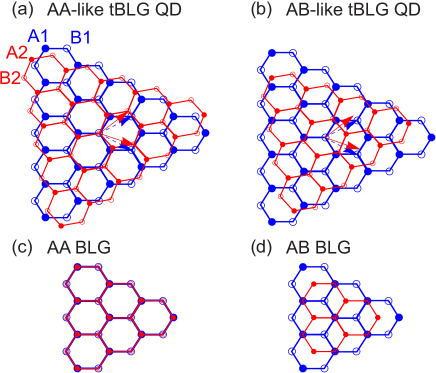
Figure 1: Schematic geometry of the triangular tBLG QDs with lateral zigzag edges. The layers are depicted in two different colors: blue (bottom) and red (top). Filled (empty) circles in each layer indicate A$i$ (B$i$) [$i=1,2$] sublattice. (a) An AA-like dot, whose untwisted arrangement corresponds to the AA-stacked triangular BLG dot [panel (c)], in which each carbon atom of the top layer is placed exactly above the corresponding atom of the bottom layer. (b) An AB-like dot, whose untwisted arrangement corresponds to the AB-stacked triangular BLG dot [panel (d)], in which different sublattices of two layers are directly coupled to each other (A1-B2) so that the two others are situated above the centers of the opposing layer hexagons (B1,A2).

At this point, it needs to be noticed that stacking two or more layers of graphene can have a significant impact on its mechanical, electronic, and magnetic properties, both in bulk and nanostructured forms, see, e.g., Refs. Velasco2014 ; Pereira2007 ; Zarenia2013 ; daCosta2015 ; Belouad2016 ; Guclu2011 ; Sahu2008 ; Henriksen2008 ; Zhang2010 ; Velasco2014 ; Fang2015 ; Rozhkov2016re ; Mirzakhani2016 ; Nascimento2017 . In the case of BLG QDs, it has been demonstrated that the edges and geometries play an essential role in modifying the energy spectrum daCosta2016a ; daCosta2016b as well as its magnetic properties Nascimento2017 , similar to monolayer graphene (MLG) QDs Zhang2008 ; Guclu2014Re . During the last decade, two well-known stacks of BLG QDs, i.e., the AA and AB types, have been experimentally realized and extensively studied Allen2012 ; Goossens2012 ; Eich2018 ; Ge2020 . Besides, the effect of twisting on the electronic and transport properties of BLG QDs has also been recently addressed both theoretically Landgraf2013 ; Tiutiunnyka2019 ; Mirzakhani2020 ; Han2020 ; Tepliakov2020 ; Wang2021 ; Wang2022 and experimentally Zhou2021 . These results, for example, suggest that the twisting axis can be utilized to tune the interlayer conductance Han2020 or that the twist angle can modify the energy levels Tiutiunnyka2019 ; Mirzakhani2020 in stacked graphene nanostructures. Despite several theoretical studies pertinent to the electronic properties of tBLG QDs, to our knowledge, there is currently no theoretical study on the magnetic properties of such QDs.

In this paper, we aim to investigate the effect of twisting angle on the magnetic properties of a triangular QD in tBLG. As previously demonstrated in Refs. Fernandez2007 ; Yazyev2010 , zigzag edges host low-energy edge states, which causes magnetism to develop in carbon nanostructures. In this study too, we only address triangular tBLG QDs with well-defined zigzag edges as shown in Fig. 1. Combining the tight-binding model (TBM) and the electron-electron (e-e) interactions addressed self-consistently at the level of the mean-field (MF) Hubbard model, we numerically investigate how twisting angle affects the magnetic ordering in (triangular) tBLG QDs. To this end, we study systematically two configurations of tBLG QDs: AA-like [Fig. 1(a)] and AB-like QDs [Fig. 1(b)], whose untwisted arrangements correspond, respectively, to the ideal AA- and AB-stacked BLG QDs, as depicted in Figs. 1(c) and 1(d).

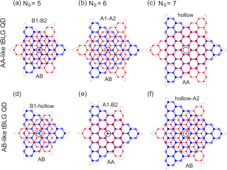
Figure 2: Geometries and geometric centers (GC, dashed circles) of three different dot sizes with the edge atoms of $N_{s}=5,6,$ and $7$ [respectively, representing $N_{s}^{(2),(3),(4)}$-group dots with $n=1$ in Eq. (1)] at a twisting angle of $\theta=60^{\circ}$ for the AA-like (upper panels) and AB-like (lower panels) dots. In each case, the GC (as the twisting point, indicated at the top of each panel) is determined by the lattice sites of the bottom and top layers where the GC is located. Notice that, at $\theta=60^{\circ}$, both dots can result in AA or AB arrangements in the layers’ intersection. The same patterns are repeated for different dot sizes, characterized by Eq. (1).

Interestingly, our numeric calculations predict a magnetic quantum phase transition at a critical twisting angle for AA-like dots. We find that the AA-like dots exhibit an antiferromagnetic phase at small twisting angles, which beyond a critical angle $\theta_{c}$ transition to a ferromagnetic phase occur for which the total spin $S$ agrees with Lieb’s theorem Lieb1989 . Lieb’s theorem predicts the total spin of the Hubbard model’s ground state in bipartite lattices. Our analysis shows that $\theta_{c}$ decreases as the dot size increases. We also find a criterion for the value of $\theta_{c}$, according to which once the maximum energy difference between electron and hole edge states in the single-particle (SP) picture is less than $(U/\gamma_{0})\times t_{0}$, the spin-polarized energy levels are aligned ferromagnetically. Here, $U$ is the Hubbard parameter and $\gamma_{0}$ ($t_{0}$) denotes the graphene intralayer (interlayer) hopping.

Unlike AA-like dots, there is no phase transition from an antiferromagnetic to a ferromagnetic phase in AB-like dots, and the spins in such dots are ferromagnetically polarized all twist angles. Furthermore, in the ferromagnetic phase, the net spin of the studied tBLG QD configurations scales linearly with dot size by one spin unit; nevertheless, AA-like dots result in an integer net spin and AB-like ones in a half-integer.

The paper is organized as follows: In Sec. II, we present the QD structures in tBLG and the basics of our numerical method. Section III is dedicated to results and discussions. A summary and concluding remarks follow in Sec. IV.

II Theory and model

In this paper, we study the intrinsic magnetism of triangular tBLG QDs for two types of configurations. Figures 1(a) and 1(b) depict two possibilities for creating a tBLG QD from two comparable monolayer QDs. A zigzag triangular tBLG QD [Figs. 1(a)], which is built from the two perfectly flat triangular MLG QDs with the same shape, size, and edge boundaries in which the second MLG QD (top) is rotated by an angle $\theta$ around the geometric center of the dot. In this case, untwisted arrangement ($\theta=0$) corresponds to an AA-stacked BLG QD configuration [Fig. 1(c)]. We will refer to such a structure as an “AA-like dot”. Another configuration choice is shown in Fig. 1(b), in which the top layer is smaller (one atom at the edge) than the bottom layer, and $\theta=0$ corresponds to a perfect AB-stacked BLG QD, see Fig. 1(d). Such a structure is referred here to as an “AB-like dot”. In both configurations, the interlayer spacing is $d_{0}=0.335$ nm. Each dot can be characterized by the number of atoms on one edge of the (bottom) layer, $N_{s}$. The total number of carbon atoms in a layer of such triangular dots with zigzag edges is $N_{L}=N_{s}^{2}+4N_{s}+1$. Notice that in zigzag triangular graphene QDs, all edge atoms belong to the same sublattice, which here is B sublattice in both layers.

Depending on the dot size, the geometric center (through which the twist axis passes) coincides at different positions, and each dot can result in either an AA- or an AB-BLG configuration when $\theta=60^{\circ}$. This feature is illustrated in Fig. 2. Accordingly, from a geometrical standpoint, we categorize the dots into three groups, identifying them by the edge atom numbers as

$$N_{s}^{(p)}=p+3n\quad(n=0,\ 1,\ \ldots),$$ (1)

where, $p=2,3,\text{and }4$. For more details, see Fig. 2 and the caption therein.

In order to study the magnetic properties of tBLG QDs, we use the widely applied one-orbital MF Hubbard model Yazyev2010 ; Fernandez2007 ; Oteyza2022 ; Wolf2021 ; Phung2022 ; Li2022 . This model considers only the unhybridized $p_{z}$ atomic orbital of the carbon atoms. The $p_{z}$-electron states govern all low-energy features of graphene, both electronic and magnetic. The Hubbard model can be expressed as the sum of two terms Hubbard1963 ,

$$\mathcal{H}=\mathcal{H}_{0}+\mathcal{H}_{\mathrm{U}}.$$ (2)

The first term ($H_{0}$) is the SP TB Hamiltonian, which in the second quantization formalism can be written as

$$\mathcal{H}_{0}=\sum_{i,\sigma}\epsilon_{i\sigma}c^{\dagger}_{i\sigma}c_{i\sigma}-\sum_{\langle i,j\rangle,\sigma}[t(\mathbf{d}_{ij})c^{\dagger}_{i\sigma}c_{j\sigma}+\text{h.c.}],$$ (3)

where $c^{\dagger}_{i\sigma}$ and $c_{i\sigma}$ are, respectively, the creation and annihilation operators for an electron on lattice site $i$ with on-site energy $\epsilon_{i\sigma}$ (we set $\epsilon_{i\sigma}=0$). $\mathbf{d}_{ij}=\mathbf{r}_{i}-\mathbf{r}_{j}$ is the distance between the lattice points ($\mathbf{r}_{i}$, $\mathbf{r}_{j}$), $t(\mathbf{d}_{ij})$ is the corresponding transfer integral, and $\langle i,j\rangle$ indicates a summation over nearest-neighbor sites. Using the Slater-Koster form, the transfer integral between the atoms $i$ and $j$ can be written as Slater1954 ; Nakanishi2001 ; Uryu2004 ; Laiss2010 ; Moon2013 ,

$$-t(\mathbf{d}_{ij})=V_{pp\pi}\Big{[}1-\Big{(}\frac{\mathbf{d}_{ij}.\mathbf{e}_{z}}{d_{ij}}\Big{)}^{2}\Big{]}+V_{pp\sigma}\Big{(}\frac{\mathbf{d}_{ij}.\mathbf{e}_{z}}{d_{ij}}\Big{)}^{2}.$$ (4)

Here, $V_{pp\pi}=\gamma_{0}\exp[-(d_{ij}-a_{cc})/\delta_{0}]$ and $V_{pp\sigma}=t_{0}\exp[-(d_{ij}-d_{0})/\delta_{0}],$ where $a_{cc}=0.142$ nm is the carbon-carbon distance of graphene and $\delta_{0}=0.184\,a$ ($a=\sqrt{3}\,a_{cc}$ is the graphene lattice constant) is the decay length. $\gamma_{0}\approx-2.7$ eV and $t_{0}\approx 0.48$ eV are the intralayer and interlayer nearest-neighbor hopping parameters, respectively. For the intralayer coupling, we include only the nearest-neighbor hopping parameter. But for the interlayer coupling, since the layers are rotated and the neighbors are not on top of each other, we take the interlayer coupling terms for atomic distances of $d_{ij}\leqslant 4a_{cc}$. For $d_{ij}>4a_{cc}$, the transfer integral is exponentially small and can be safely ignored Moon2013 . The electron-hole symmetry is also broken as a result of the mixing between the two sublattices.

The second term in Hamiltonian (2) is the Hubbard term that introduces e-e interactions through the repulsive on-site Coulomb interaction,

$$\mathcal{H}_{\mathrm{U}}=U\sum_{i}n_{i\uparrow}n_{i\downarrow},$$ (5)

where $n_{i\sigma}=c^{\dagger}_{i\sigma}c_{i\sigma}$ ($\sigma=\uparrow,\downarrow$) is the spin-resolved electron density at site $i$. The parameter $U>0$ is the Hubbard parameter and denotes, in the short-range regime, the on-site Coulomb repulsion energy for each pair of electrons with opposite spins on the same site $i$.

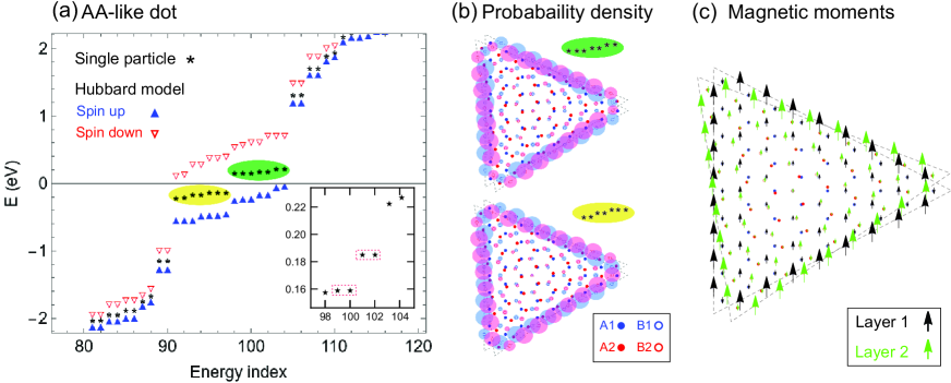
Figure 3: (a) Energy levels of an AA-like triangular tBLG QD with $N_{s}=8$ and twisting angle of $\theta=7^{\circ}$ in the frame of SP (single particle, black stars) and Hubbard model (triangles) around the Fermi energy $E_{f}=0$. Filled blue (empty red) triangles depict the spin up (down) energy levels. The inset shows a zoom of the LUMO cluster energy levels (encircled by the green oval in the main figure), indicating two doubly degenerate (red boxes) and three non-degenerate energy levels. (b) Probability densities corresponding to two clusters of the LUMO (upper panel) and HOMO (lower panel) energy levels around $E_{f}$. (c) Local magnetic moments $m_{i}$ shown by the black and green arrows corresponding to the lower and upper layers, respectively. The length of the arrows signifies the relative magnitude of the magnetic moments.

In the MF approximation, the Hubbard term (5) at half-filling can be rewritten as

$$\mathcal{H}_{\mathrm{U}}=U\sum_{i}\big{(}n_{i\uparrow}-\frac{1}{2}\big{)}\big{(}n_{i\downarrow}-\frac{1}{2}\big{)}\\ =U\sum_{i}\big{[}\langle n_{i\downarrow}\rangle n_{i\uparrow}+\langle n_{i\uparrow}\rangle n_{i\downarrow}-\frac{1}{2}(n_{i\uparrow}+n_{i\downarrow})-\langle n_{i\uparrow}\rangle\langle n_{i\downarrow}\rangle+\frac{1}{4}\big{]}.$$ (6)

Here, a spin-up electron, $n_{i\uparrow}$, at site $i$ interacts with the average density of spin-down electrons $\langle n_{i\downarrow}\rangle$ at the same site and vice versa. Accordingly, the MF Hubbard Hamiltonian only contains SP operators. It is also worth mentioning that such MF approximation shows the Hartree term, that is, the MF Hubbard term is only written for the $z$ component of the spin moment. This is the most common method for examining a system’s magnetic properties Yazyev2010 ; Fernandez2007 ; Oteyza2022 .

To solve the problem for $\mathcal{H}$, we use self-consistent calculations that start with randomly chosen initial values for the unknown electron densities $\langle n_{i\sigma}\rangle$. The Hamiltonian (2) is then diagonalized to obtain the new eigenvalues and eigenvectors, which are used to compute the new spin densities $\langle n_{i\uparrow}\rangle$ and $\langle n_{i\downarrow}\rangle$ on each site. Then, the obtained new spin densities are fed as the initial values for the next iteration. The procedure is repeated until all values of $\langle n_{i\sigma}\rangle$ are converged. The convergency criterion is met when $\langle n_{i\sigma}\rangle^{s+1}-\langle n_{i\sigma}\rangle^{s}<\delta$, where $\delta$ is a small number chosen $\delta=10^{-6}$ and $s$ is the self-consistent cycle index. After achieving self-consistency, one can compute the magnetic moment per atomic site

$$m_{i}=\frac{\langle n_{i\uparrow}\rangle-\langle n_{i\downarrow}\rangle}{2},$$ (7)

and the total spin of system $S=\sum_{i}m_{i}$.

From literature (see, e.g., Refs. Yazyev2010 ; Nascimento2017 ), there is currently no consensus on the exact value of $U$ in the case of graphene-based structures. Such a parameter should ideally be approximated using experimental data, and there are currently no standard or direct experiments on magnetic graphene systems to which we may refer. However, it has been demonstrated that for specific values of $U/|\gamma_{0}|$, the results of MF Hubbard model calculations are in good agreement with results from first-principles approaches based on density functional theory Fernandez2007 ; Pisani2007 ; Gunlycke2007 . In general, the most common range of $U$ parameter values is $U\sim 3.0-3.5$ eV, which corresponds to $U/|\gamma_{0}|\sim 1.1-1.3$ Yazyev2010 .† At $U/|\gamma_{0}|\approx 2.23$, ideal graphene undergoes a Mott-Hubbard transition into an antiferromagnetically ordered insulating phase Sorella1992 ; Fujita1996 . In our calculations, we use the value of $U=1.2\,|\gamma_{0}|=3.24$ eV, unless otherwise specified.

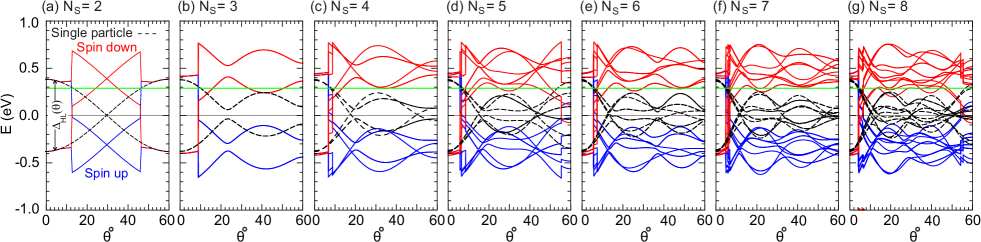
Figure 4: Energy levels of the AA-like dot as a function of the twist angle $\theta$ for different dot sizes as indicated by the $N_{s}$ value in each panel. The results are presented for SP (dashed black curves) and Hubbard models [spin up (blue) and spin down (red)] around the Fermi energy $E_{f}=0$. The solid green lines indicate $(q\times t_{0})/2$ [$q\equiv U/|\gamma_{0}|=1/2$; explained in Eq. (9)]. As clearly seen, when $\Delta_{HL}(\theta)/2$ falls below the green line, the energy levels become spin polarized in all cases.

Figure 5: (a) Total spin $S$ as a function of $\theta$ for AA-like dots whose energy levels are shown in Fig. 4. For certain twisting angles, $S$ achieves a value that is consistent with Lieb’s theorem prediction [Eq. (8)].¬† (b) Local magnetic moments for a dot with $N_{s}=5$ and $\theta=5.5^{\circ}$, presenting an antiferromagnetic phase with $S=0$, as seen in panel (a).

III Numerical results

III.1 AA-like triangular tBLG QDs

First, we consider the AA-like dots as illustrated in Fig. 1(a). Figure 3(a) shows the energy spectrum of an AA-like dot with $N_{s}=8$ edge atoms and a twist angle of $\theta=7^{\circ}$ as a function of the energy index. The results are presented for the SP (black stars) and the MF Hubbard models near the Fermi energy $E_{f}=0$. Filled (empty) triangular symbols correspond to the spin up (down) energy states. As seen, in the case of SP energy levels, there are two clusters of nearly-degenerate energy levels [indicated by yellow and green ovals in Fig. 3(a)] corresponding to the highest occupied and lowest unoccupied molecular orbitals (HOMOs and LUMOs) around $E_{f}=0$. Such electronic states originate from sublattice imbalance of each layer of the dot. In a bipartite structure, one can find $N_{Z}$ “strict” zero-energy states (according to the “benzenoid graph” theory Fajtlowicz2005 ) equating to sublattice imbalance $|N_{A}-N_{B}|$, where $N_{A}$ and $N_{B}$ are the number of sites in sublattices A and B, respectively Yazyev2010 ; Oteyza2022 . In the case of zigzag triangular MLG QDs, the sublattice imbalance is proportional to the number of atoms at one edge, i.e., $|N_{A}-N_{B}|=N_{s}-1=N_{Z}$ Potasz2010 . Here, two clusters of $N_{Z}=7$ nearly-degenerate energy states (totally 14 states) appear around $E_{f}$, due to the two triangular MLG QDs, which are gaped as a result of the interlayer coupling between the edge atoms of the two dot layers. The SP energy gap is $\Delta_{SP}\approx 0.28$ eV. Notice that each cluster of energies consists of two doubly degenerate and three non-degenerate states as shown in the inset of Fig. 3(a). Probability densities corresponding to each cluster of electron and hole energy states [Fig. 3(b)] show that all states are mostly localized at the edges of the dot and are sublattice polarized as well. Here, because atoms of the dot edges belong to the B-sublattice, carriers are only localized at the B atoms [open circles in Fig. 3(b)]. Furthermore, the probability densities of each energy cluster are almost evenly distributed between the two layers.

Including the MF Hubbard model, one can see that each (spin-degenerate) energy state is now spin polarized. Filled blue (empty red) symbols in Fig. 3(a) show the spin up (down) energy levels. As seen, each energy state in the two HOMOs and LUMOs clusters are considerably affected by the e-e interaction. However, the same type of SP energy degeneracy is still preserved for each spin-polarized energy levels. The spin-polarized energy gap is $\Delta_{H}\approx 0.15$ eV. Local magnetic moments $m_{i}$, shown in Fig. 3(c), demonstrate that the two layers are ferromagnetically coupled to each other, and each layer shares the same magnetization behavior. However, the magnetic moments of the two sublattices in each layer are antiferromagnetic ordered. Further, the moments corresponding to the edges’ atoms are the largest, which decay to zero in the center of the dot. The same behavior was also seen in both triangular MLG and AA-stacked BLG QDs Fernandez2007 ; Nascimento2017 . The total spin of the dot is $S=7$, which agrees with Lieb’s theorem, which states that a bipartite system described by the Hubbard model at half-filling displays a ground state with a net spin of magnitude Lieb1989

$$S=\frac{1}{2}|N_{A}-N_{B}|.$$ (8)

This theorem allows us to predict the spin of the ground state of the bipartite molecular systems, such as graphene-based nanostructures, only by counting the sublattice imbalance $|N_{A}-N_{B}|$.

After investigating the energy states for a particular AA-like dot, now we examine the effect of twisting angle $\theta$ on the variation of the energy levels as a function of $\theta$ for fixed dot sizes. Figure 4 shows the lowest energy levels around $E_{f}=0$ for different dot sizes with the number of edge atoms $N_{s}=2,3,\ldots,$ and $8$. The results depict the two clusters of the HOMOs and LUMOs of the SP framework (black dashed) and the corresponding spin-polarized energy levels [spin up (blue) and spin down (red)] of the Hubbard model. First, notice that the SP energy spectrum features an equal opening energy gap independent of the dot sizes when $\theta=0$, which corresponds to the AA-stacked configuration of the triangular tBLG QD. The size of the SP energy gap at $\theta=0$ is $\Delta_{SP}=\epsilon^{+}-\epsilon^{-}=0.74$ eV, ($\epsilon^{\pm}\approx\pm 0.37$ eV), which is the largest value for the entire range of twist angle. This is expected since the untwisted structure (AA stacking) has the largest interlayer coupling between edge atoms, see Fig. 1(c). However, as seen in Fig. 4, increasing the twisting angle leads the energy gap to shrink and close (or become minimum) at certain values of $\theta$. Notice that the gap decreases quickly and exhibits an oscillatory behavior for large dot sizes as the twist angle increases. Further, the maximum energy separation between HOMOs and LUMOs at $\theta=60^{\circ}$ occurs for $N_{s}^{(2)}$-group QDs, as seen for $N_{s}=2,5$ and $8$ in Figs. 4(a), 4(d), and 4(g), respectively. This can be understood by the edge atoms’ coupling, whose $N_{s}^{(2)}$-group dots are greater than those of the two others. In this case, as seen in Fig. 2(a), the edge atoms of each layer are directly connected to the atoms of the adjacent layer that belong to the sublattice of the edge atoms, i.e. B1-B2. As previously shown, the HOMOs and LUMOs probability densities are sublattice polarized and solely localized at the B1 and B2 sublattices, which leads to a strong coupling between the layers in $N_{s}^{(2)}$-group dots.

The corresponding total spin $S$ for the dots with the spin-polarized energy levels shown in Fig. 4, is plotted in Fig. 5(a). All dot sizes for small twist angles (which decrease as dot size increases) have a total spin of $S=0$ and the magnitude of $S$ is consistent with Lieb’s theorem [Eq. (8)] for large twisting angles. The observed behavior for small twisting angles does not contradict the prediction of Lieb’s theorem, but rather indicates that the energy levels at these angles are antiferromagnetically polarized, as can be seen directly from the energy spectra shown in Fig. 4. This antiferromagnetic spin alignment can be highlighted further by plotting the local magnetic moments for an example of dot size and twist angle, e.g., $N_{s}=5$ and $\theta=5.5^{\circ}$ [Fig. 5(b)]. As seen, the spin polarization of each layer is oriented equally in opposite directions. Accordingly, all dot sizes exhibit a critical value of twist angle ($\theta_{c}$), at which a magnetic phase transition occurs. As visible in Fig. 5(a), $\theta_{c}$ decreases as the dot size increases.

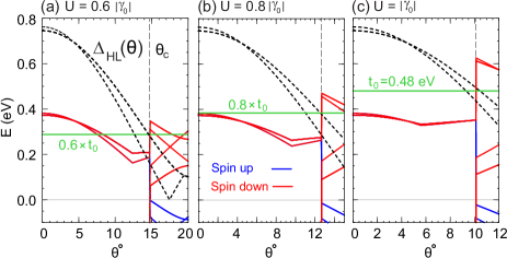
Figure 6: A zoom of the energy levels for an AA-like tBLG dot with $N_{s}=4$, as a function of $\theta$ for three different values of the Hubbard parameter ($U=q\,|\gamma_{0}|$) (a) $q=0.6$, (b) $q=0.8$, and (c) $q=1$. As seen, when the maximum energy difference between two clusters of HOMOs and LUMOs ($\Delta_{HL}(\theta)$; dashed curves) goes below $q\times t_{0}$ (green lines), the energy levels become spin polarized.

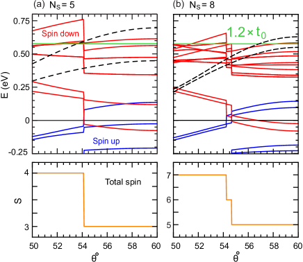
Figure 7: (Upper panel) A zoom of the lowest spin-polarized energy levels of AA-like dots with (a) $N_{s}=5$ and (b) $N_{s}=8$ for the twist angle range of $[50^{\circ},~{}60^{\circ}]$. Dashed black curves show the energy gap of the two outmost SP HOMOs and LUMOs, and the horizontal solid green line indicates $q\times t_{0}$ ($q=1.2$). (Lower panel) The corresponding total spin $S$ for each dot.†

Our numerical calculations demonstrate that the phase transition occurs when the ratio of the (maximum) energy difference between the HOMOs and LUMOs (in the SP frame), $\Delta_{HL}(\theta)$, to the interlayer coupling $t_{0}$ becomes lesser than the ratio of the Hubbard parameter $U$ to the intralayer hopping $|\gamma_{0}|$, i.e.,

$$\Delta_{HL}(\theta)\lessapprox q\times t_{0},$$ (9)

where $q=U/|\gamma_{0}|$. To highlight this point, we plot, in Fig. 6, a zoom of the Hubbard spin-polarized energy levels and $\Delta_{HL}(\theta)$ for a dot with $N_{s}=4$ and different Hubbard parameter values ($U=q\,|\gamma_{0}|$), e.g., (a) $q=0.6$, (b) $q=0.8$, and (c) $q=1$. As seen, the above-mentioned criterion is met in all cases. This behavior is also visible in the energy levels depicted in Fig. 4 for different dot sizes but with the constant $U=1.2\,\gamma_{0}$ value. Magnetic phase transition occurs for all dots when $\Delta_{HL}(\theta)/2$ falls below $(q\times t_{0})/2\approx 0.29$ eV (here $q=1.2$); notice the horizontal green lines in all panels of Fig. 4 and the caption therein.

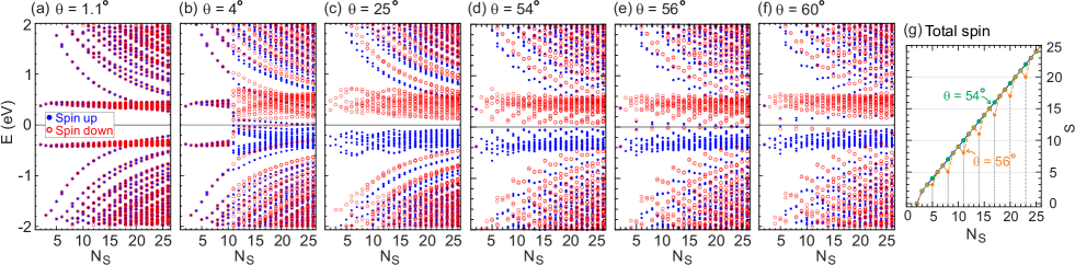
Figure 8: (a-f) Spin-polarized energy levels of the AA-like dot as a function of dot size, characterized by $N_{s}$, around the Fermi energy $E_{f}=0$ for six different twist angles as indicated in each panel. Filled blue (empty red) circles represent spin-up (spin-down) energy levels.† (g) Net spin plotted for two twist angles of $\theta=54^{\circ}$ (green) and $\theta=56^{\circ}$ (orange). The vertical dashed gray lines indicate $N_{s}^{(2)}$-group dots, whose net spin deviates from Lieb’s theorem prediction beyond the twist angle of $\theta\simeq 55^{\circ}$.

The spin-polarized energy levels exhibit smooth variation as a function of $\theta$ in the ferromagnetic phase for which the total spin $S$ of the structures agrees with the prediction of Lieb’s theorem, as shown in Fig. 5(a). Notice that the net spin scales linearly with dot size by one spin unit. While the $N_{s}^{(3),(4)}$-group dots exhibit a smooth variation of the energy spectra as the twist angle approaches $\theta=60^{\circ}$, the energy levels of the $N_{s}^{(2)}$-group dots, i.e., $N_{s}=2,5,$ and $8$, undergo an abrupt decline in this area as seen in Figs. 4(a), 4(d) and 4(g), respectively. Such abrupt drops in the energy levels are manifested as a decrease in the total spin of the dot by one or two units depending on the dot sizes, as shown in Fig. 5(a).† Figure 7 shows a zoomed of the energy levels for two examples of these types of dots, i.e., $N_{s}=5$ (a) and $N_{s}=8$ (b), at twist angles between $50^{\circ}\leq\theta\leq 60^{\circ}$. As seen, the abrupt decrease in energy levels around the twist angle of [$54^{\circ}$- $56^{\circ}$] results in an antiferromagnetically polarization of the lowest energy level(s). This is a generic feature for $N_{s}^{(2)}$-group dots which will be discussed latter in Figs. 8(d) and 8(e). We attribute this behavior to the criterion mentioned in Eq. (9). As depicted in Fig. 7, once $\Delta_{HL}(\theta)$ (dashed black curves shown only for the two outermost HOMOs and LUMOs) exceeds $q\times t_{0}$ ($\approx 0.58$ eV, green line), a decline in the energy levels occur. This criterion is well matched in the case of $N_{s}=5$ [Fig. 7(a)], but there is some discrepancy for $N_{s}=8$ [Fig. 7(b)].

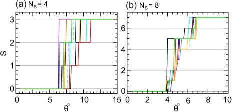
Figure 9: Total spin as a function of $\theta$ shown for ten different randomly chosen initial electron densities $\langle n_{i\sigma}\rangle$ for two AA-like dot sizes (a) $N_{s}=4$ and (b) $N_{s}=8$. †

It is also interesting to discuss the dependence of magnetization on the dot size. Figures 8(a)-8(f) show the lowest energy levels as a function of the dot size (characterized by $N_{s}$) for the six different twist angles $\theta=1.1^{\circ},\ 4^{\circ},\ 25^{\circ},\ 54^{\circ},\ 56^{\circ}$, and $60^{\circ}$. The results are shown up to $N_{s}=26$. As seen, for tiny twist angles, e.g., $\theta=1.1^{\circ}$, the energy levels show antiferromagnetic polarization for the entire range of dot sizes. In the case of $\theta=4^{\circ}$ [Figs. 8(b)], small dots exhibit antiferromagnetic phase and turn to ferromagnetic phase when dot size increases, around $N_{s}=11$. This is because of the fast decline in the SP energy gap for the large dot sizes. At intermediate twist angles, such as $\theta=25^{\circ}$ [Fig. 8(c)], the energy levels are perfectly aligned ferromagnetically; two clusters of spin-polarized HOMOs and LUMOs are formed around the Fermi energy $E_{f}=0$, where the energy gap diminishes smoothly as the dot size increases. This ferromagnetic phase is maintained for all dot sizes until $\theta\approx 55^{\circ}$, as seen in Fig. 8(d). However, beyond the angle $\theta\approx 55^{\circ}$ [Figs. 8(e) and 8(f)], the $N_{s}^{(2)}$-group dots behave differently from the other two groups, with the lowest one or two energy levels being antiferromagnetically polarized, resulting in a drop in the net spin of the dots. To highlight this further, total spin as a function of $N_{s}$ is shown in Fig. 8(g) for two twist angles $\theta=54^{\circ}$ (green) and $\theta=56^{\circ}$ (orange). As seen, while the net spin of all dots scales linearly at $\theta=54^{\circ}$, the $N_{s}^{(2)}$-group dots (marked by dashed gray vertical lines) show a reduced net-spin value from Lieb’s theorem prediction for $\theta=56^{\circ}$. Except for $N_{s}=2$, which displays one unit reduction, the remaining $N_{s}^{(2)}$-group dots show a net spin of two units less than what Lieb’s theory predicts.

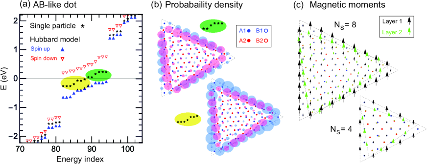
Figure 10: (a) Energy spectra of an AB-like dot with $N_{s}=8$ and a twist angle of $\theta=7^{\circ}$ in the frame of SP (black stars) and Hubbard models around the Fermi energy $E_{f}=0$. Filled blue (empty red) symbols depict the up (down) energy levels. (b) Probability densities corresponding to two clusters of the LUMOs (upper panel) and HOMOs (lower panel). Bottom (top) layer is represented by the light blue (red) color. (c) Local magnetic moments $m_{i}$ for two examples of AB-like dots of $N_{s}=8$ and $N_{s}=4$ ($\theta=7^{\circ}$) are shown by the black and green arrows corresponding to the lower and upper layers, respectively. The length of the arrows is measure of the relative magnitude of the magnetic moments.†

At this point it is worth mentioning that all MLG carbon nanostructures studied in previous literature feature zero-energy states for which any repulsive Coulomb interaction can cause spin-polarization, a mechanism for escaping an instability caused by the presence of low-energy electrons in the system Yazyev2010 ; Oteyza2022 . As illustrated above, an AA-like dot no longer features strictly zero-energy states at small twist angles. However, the same scenario occurs with such graphene QDs. For small twist angles near the AA-stacking configuration, it is energetically favorable for spins in adjacent layers to couple to each other antiferromagnetically. Increasing the twisting angle, HOMO and LUMO electronic states approach the Fermi level; in the case when the Coulomb repulsion and energy separation between HOMOs and LUMOs meet the criterion expressed by Eq. (9), the energy levels become spin polarized to reduce the density of states around the Fermi energy. Furthermore, notice that, where the HOMOs and LUMOs are closer to the Fermi level at $E_{f}=0$, spin-polarized energy levels are formed farther away, and vice versa, see Fig. 4.

We also would like to point out an issue in the numerical calculation using the MF Hubbard model for the studied dots. Our findings show that the results for the critical values of twist angles at which the magnetic phase transition occurs can be varied depending on the randomly chosen initial values for the electron densities $\langle n_{i\sigma}\rangle$. For example, in Fig. 9, we plot the net spin for two examples of the AA-like dots with (a) $N_{s}=4$ and (b) $N_{s}=8$ for ten different randomly chosen electron densities $\langle n_{i\sigma}\rangle$. As seen, the critical twist angles change slightly for different initial values of $\langle n_{i\sigma}\rangle$, and these variations appear to diminish as the dot size increases, cf. Figs 9(a) and 9(b). All cases, however, share a similar thread.

III.2 AB-like triangular tBLG QDs

Now we investigate the magnetic properties of AB-like tBLG QD, whose configuration is illustrated in Fig. 1(b). In this configuration, the top layer is smaller than the bottom layer by one edge atom, and $\theta=0^{\circ}$ corresponds to the AB-stacking BLG QD [Fig. 1(d)]. In BLG, the AB stacking configuration is more natural and stable than the AA arrangement. As we discuss below, such a BLG dot features an odd number of degenerate edge states that can generate a half-integer net spin in contrast to the AA-like dots with an integer net spin.

Figure 10(a) shows the energy levels for an example of AB-like tBLG QDs with the same parameters as used for the AA-like dot of previous section [Fig. 3(a)], i.e., $N_{s}=8$ and $\theta=7^{\circ}$. Here also, the number of SP edge states is consistent with the benzenoid graph theory. As seen, there are $13$ edge states (black stars): $N_{Z}=7$ (encircled in the yellow oval) from the bottom layer and $N_{Z}=6$ (green oval) from the upper layer. Notice that here the edge states are more dispersed compared to those in the AA-like configuration [cf. Figs. 3(a) and 10(a)]. The SP energy gap is $\Delta_{SP}\approx 0.08$ eV, which is smaller than for the AA-like dot by a factor of $3.5$. This is related to the coupling between edge atoms, which is weaker in the AB-like dots.† The probability densities corresponding to each layer’s edge states are mostly concentrated in the same layer [Fig. 10(b)], as opposed to the AA-like dot, whose edge states are almost evenly distributed in both layers due to layer symmetry [Fig. 3(b)]. However, the edge-state densities in both types of dots are sublattice polarized.

Similar to the case of the AA-like dot, including MF on the level of the Hubbard model, the edge states are considerably affected by the e-e interaction. Here, the spin-polarized energy gap is about $\Delta_{H}\approx 0.60$ eV, which is four times larger than that in the AA-like dot. The local magnetic moments are depicted in Fig. 10(c), demonstrating that in the bottom layer they are somewhat larger than that in the top layer. This feature is more pronounced for small dot sizes as shown in Fig. 10(d) for a dot with $N_{s}=4$.

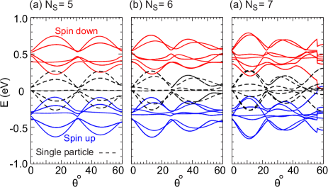
Figure 11: Energy levels of the AB-like dots as a function of twist angle $\theta$ for three different dot sizes as indicated by the number $N_{s}$ of edge atoms in each panel. Dashed black curves are for SP model, and blue and red ones show the spin up and spin down energy levels in the Hubbard model.†

In Fig. 11, we show the the lowest energy levels around $E_{f}=0$ for three dot sizes of the AB-like dots with the edge atoms of (a) $N_{s}=5$, (b) $N_{s}=6$, and (c) $N_{s}=7$, respectively, representing $N_{s}^{(2),(3),(4)}$-group dots [Eq. (1)]. As seen, all dots exhibit ferromagnetically-polarized energy levels throughout the whole twist angle range of $[0,60^{\circ}]$, with the net spin $S$ consistent with Lieb’s theorem prediction. The numerically calculated total spins are shown in each panel. Notice that because of the one edge atom discrepancy between the bottom and top layers in the AB-like dots, the total spins come out as half-integer numbers. However, here too, the $N_{s}=7$ dot (an example of $N_{s}^{(4)}$-group dots) undergo abrupt drops in the energy levels when the twist angle approaches $\theta=60^{\circ}$. This behavior is analogous to that of the $N_{s}^{(2)}$ group of the AA-like dots, as explained in Fig. 7. This is to be expected as we can see from the geometries in Figs. 2(a) and 2(f), which are both similar around $\theta=60^{\circ}$.

Finally, we conclude this section by mentioning a few words about the magnetism in MLG and BLG nanostructures. In contrast to MLG triangle QDs Yazyev2010 , where the total spin scales linearly with dot size by half a spin unit, i.e., $S=1/2,1,3/2,\ldots$, the examples above show that the $S$ for both tBLG QD configurations in the ferromagnetic phase scales linearly with dot size by one spin unit. However, as discussed above, AA-like and AB-like dots feature integer ($S=1,2,3,\ldots$) and half-integer ($S=3/2,5/2,\ldots$) total spin, respectively. A striking feature of a tBLG QD is its capacity to control the position of its energy levels by tuning the relative twist angle of the layers while still representing a specific spin. Besides, the prediction of a magnetic quantum phase transition at a critical twisting angle would be of interest for understanding the fundamental physics of magnetism in tBLG dots, as well as for potential applications in areas such as spintronics and quantum computing.

IV Conclusion

In conclusion, using the TBM in combination with the MF Hubbard model, we studied the magnetic properties of zigzag-edged triangular QDs in tBLG with a focus on the effects of variations in the twist angle as well as dot size. We considered two configurations of tBLG QDs: AA-like and AB-like QDs, whose untwisted arrangements correspond, respectively, to the AA- and AB-stacked BLG QDs. Depending on the dot size, such QDs would have a different geometries, and we classified them appropriately into three categories.

Our findings show that the AA-like dots exhibit an antiferromagnetic phase for small twist angles, which transits to a ferromagnetic phase beyond a critical value of $\theta_{c}$.† Our analysis shows that the size of $\theta_{c}$ decreases as the dot size increases. We also found a criteria for such $\theta_{c}$, according to which the dots exhibit ferromagnetic spin polarization as long as the energy difference between the electron and hole edge states (in the single particle frame) is less than $(U/\gamma_{0})\times t_{0}$, where $U$ is the Hubbard e-e interaction and $\gamma_{0}$ ($t_{0}$) denotes the graphene intralayer (interlayer) hopping. Unlike AA-like dots, spins in the AB-like dots are ferromagnetically polarized for the entire range of twist angle. The net spin $S$ of both types of QDs in the ferromagnetic phase is consistent with the prediction from Lieb’s theorem, where AA-like (AB-like) dot exhibits an integer (half-integer) total spin value.

Due to the dispersive and oscillatory behavior of the energy levels as a function of twist angle in such QDs, the ferromagnetic phase is preserved as long as the energy gap between the edge states is satisfied by the above-mentioned criterion. Our analysis showed that depending on whether the entire or part of such gaps surpass the amount of $(U/\gamma_{0})\times t_{0}$, the spins can be polarized antiferromagnetically with $S=0$ or ferromagnetically with a finite $S$ (an integer multiple of 1/2) less than Lieb’s theorem prediction. For the applied Hubbard e-e interaction here ($U=1/2\,\gamma_{0}$), the latter property occurred for a group of both types of dots at the twist angle range of $[55^{\circ}-60^{\circ}]$, i.e., when two triangular layers are almost overlapped in the opposite direction, as in the “David star” configuration.

Using the twist angle as a knob to tune the energy levels of QDs in tBLG presents an interesting opportunity to manipulate the charge and spins in such nanostructures, which are promising candidates for future electronic and spintronic technologies.

References

- (1) A. K. Geim and K. S. Novoselov Nat. Mater. 6, 183 (2007).
- (2) A. H. Castro Neto, F. Guinea, N. M. R. Peres, K. S. Novoselov, and A. K. Geim, Rev. Mod. Phys. 81, 109 (2009).
- (3) M. A. H. Vozmediano, M. I. Katsnelson, and F. Guinea, Phys. Rep. 496, 109 (2010).
- (4) K. S. Novoselov, A. K. Geim, S. V. Morozov, D. Jiang, Y. Zhang, S. V. Dubonos, I. V. Grigorieva, and A. A. Firsov, Science 306, 666 (2004).
- (5) K. Nakada, M. Fujita, G. Dresselhaus, and M. S. Dresselhaus, Phys. Rev. B 54, 17954 (1996).
- (6) Y.-W. Son, M. L. Cohen, and S. G. Louie, Phys. Rev. Lett. 97, 216803 (2006); Erratum, Phys. Rev. Lett. 98, 089901 (2007).
- (7) J. Fernández-Rossier and J. J. Palacios, Phys. Rev. Lett. 99, 177204 (2007).
- (8) O. V. Yazyev, Rep. Prog. Phys. 73, 056501 (2010).
- (9) P. Potasz, A. D. Güçlü, A. Wójs, and P. Hawrylak Phys. Rev. B 85, 075431 (2012).
- (10) D. G. de Oteyza and T. Frederiksen, J. Phys.: Condens. Matter 34, 443001 (2022).
- (11) E. J. Duplock, M. Scheffler, and P. J. D. Lindan, Phys. Rev. Lett. 92, 225502 (2004).
- (12) J. J. Palacios, J. Fernández-Rossier, and L. Brey, Phys. Rev. B 77, 195428 (2008).
- (13) M. M. Ugeda, I. Brihuega, F. Guinea, and J. M. Gómez-Rodríguez, Phys. Rev. Lett. 104, 096804 (2010).
- (14) H. González-Herrero, J. M. Gómez-Rodríguez, P. Mallet, M. Moaied, J. J. Palacios, C. Salgado, M. M. Ugeda, J. Y. Veuillen, F. Yndurain, and I. Brihuega, Science 352, 437 (2016).
- (15) N. Pavliček, A. Mistry, Z. Majzik, N. Moll, G. Meyer, D. J. Fox, and L. Gross, Nat. Nanotechnol. 12, 308 (2017).
- (16) S. Mishra, D. Beyer, K. Eimre, J. Liu, R. Berger, O. Gröning, C. A. Pignedoli, K. Müllen, R. Fasel, X. Feng, and P. Ruffieux J. Am. Chem. Soc. 141, 10621 (2019).
- (17) J. Su, M. Telychko, P. Hu, G. Macam, P. Mutombo, H. Zhang, Y. Bao, F. Cheng, Z.-Q. Huang, Z. Qiu, S. J. R. Tan, H. Lin, P. Jelínek, F.-C. Chuang, J. Wu, and J. Lu, Sci. Adv. 5, 7717 (2019).
- (18) S. Mishra, D. Beyer, K. Eimre, S. Kezilebieke, R. Berger, O. Gröning, C. A. Pignedoli, Klaus Müllen, P. Liljeroth, P. Ruffieux, X. Feng, and R. Fasel, Nat. Nanotechnol. 15, 22 (2020).
- (19) C. Tao, L. Jiao, O. V. Yazyev, Y.-C. Chen, J. Feng, X. Zhang, R. B. Capaz, J. M. Tour, A. Zettl, S. G. Louie, H. Dai, and M. F. Crommie, Nat. Phys. 7, 616 (2011).
- (20) P. Ruffieux, S. Wang, B. Yang, C. Sánchez-Sánchez, J. Liu, T. Dienel, L. Talirz, P. Shinde, C. A. Pignedoli, D. Passerone, T. Dumslaff, X. Feng, K. Müllen, and R. Fasel, Nature 531, 489 (2016).
- (21) A. L. Sharpe, E. J. Fox, A. W. Barnard, J. Finney, K. Watanabe, T. Taniguchi, M. A. Kastner, and D. Goldhaber-Gordon, Science 365, 605 (2019).
- (22) J. Liu and X. Feng, Angew. Chem. Int. Ed. 59, 23386 (2020).
- (23) S. Song, J. Su, M. Telychko, J. Li, G. Li, Y. Li, C. Su, J. Wu, and J. Lu, Chem. Soc. Rev. 50 3238 (2021).
- (24) J. Velasco, Y. Lee, Z. Zhao, L. Jing, P. Kratz, M. Bockrath, and C.N. Lau, Nano Lett. 14, 1324 (2014).
- (25) W. Fang, A. L. Hsu, Y. Song, and J. Kong, Nanoscale 7, 20335 (2015).
- (26) E.A. Henriksen, Z. Jiang, L.-C. Tung, M.E. Schwartz, M. Takita, Y.-J. Wang, and P. Kim, H.L. Stormer, Phys. Rev. Lett. 100, 087403 (2008).
- (27) A. V. Rozhkov, A. O. Sboychakov, A. L. Rakhmanov, and F. Nori, Phys. Rep. 648, 1 (2016).
- (28) J. M. Pereira, P. Vasilopoulos, and F. M. Peeters, Nano Lett. 7, 946 (2007).
- (29) B. Sahu, H. Min, A.H. MacDonald, and S.K. Banerjee, Phys. Rev. B 78, 045404 (2008).
- (30) A. D. Güçlü, P. Potasz, and P. Hawrylak, Phys. Rev. B 84, 035425 (2011).
- (31) Z. Zhang, C. Chen, X.C. Zeng, and W. Guo, Phys. Rev. B 81, 155428 (2010).
- (32) M. Zarenia, B. Partoens, T. Chakraborty, and F. M. Peeters, Phys. Rev. B 88, 245432 (2013).
- (33) D. R. da Costa, M. Zarenia, A. Chaves, G. A. Farias, and F. M. Peeters, Phys. Rev. B 92, 115437 (2015).
- (34) A. Belouad, Y. Zahidi, and A. Jellal, Mater. Res. Express. 3, 055005 (2016).
- (35) M. Mirzakhani, M. Zarenia, S. A. Ketabi, D. R. da Costa, and F. M. Peeters, Phys. Rev. B 93, 165410 (2016).
- (36) J. S. Nascimento, D. R. da Costa, M. Zarenia, Andrey Chaves, and J. M. Pereira Jr., Phys. Rev. B 96, 115428 (2017).
- (37) D. R. da Costa, M. Zarenia, Andrey Chaves, J. M. Pereira, Jr., G. A. Farias, and F. M. Peeters, Phys. Rev. B 94, 035415 (2016).
- (38) D. R. da Costa, M. Zarenia, Andrey Chaves, G. A. Farias, and F. M. Peeters, Phys. Rev. B 93, 085401 (2016).
- (39) Z. Z. Zhang, K. Chang, and F. M. Peeters, Phys. Rev. B 77, 235411 (2008).
- (40) A. D. Güçlü, P. Potasz, M. Korkusinski, P. Hawrylak, X. Li, S. P. Lau, L. Tang, R. Ji, and P. Yang, Graphene Quantum Dots, (Springer, Berlin, 2014).
- (41) M. T. Allen, J. Martin, and A. Yacoby, Nat. Commun. 3, 934 (2012).
- (42) A. M. Goossens, S. C. M. Driessen, T. A. Baart, K. Watanabe, T. Taniguchi, and L. M. K. Vandersypen, Nano Lett. 12, 4656 (2012).
- (43) M. Eich, F. Herman, R. Pisoni, H. Overweg, A. Kurzmann, Y. Lee, P. Rickhaus, K. Watanabe, T. Taniguchi, M. Sigrist, T. Ihn, and K. Ensslin, Phys. Rev. X 8, 031023 (2018).
- (44) Z. Ge, F. Joucken, E. Quezada, D. R. da Costa, J. Davenport, B. Giraldo, T. Taniguchi, K. Watanabe, N. P. Kobayashi, T. Low, and J. Velasco, Nano Lett. 20, 8682 (2020).
- (45) W. Landgraf, S. Shallcross, K. Türschmann, D. Weckbecker, and O. Pankratov, Phys. Rev. B 87, 075433 (2013).
- (46) A. Tiutiunnyka, C. A. Duqueb, F. J. Caro-Loperac, M. E. Mora-Ramosa, and J. D. Correac, Phys. E 112, 36 (2019).
- (47) M. Mirzakhani, F. M. Peeters, and M. Zarenia, Phys. Rev. B 101, 075413 (2020).
- (48) Y. Han, J. Zeng, Y. Ren, X. Dong, W. Ren, and Z. Qiao, Phys. Rev. B 101, 235432 (2020).
- (49) N. V. Tepliakov, A. V. Orlov, E. V. Kundelev, and I. D. Rukhlenko, J. Phys. Chem. C 124, 22704 (2020).
- (50) X. Wang, Y. Cui, L. Zhang, and M. Yang, Nano Res. 14, 3935 (2021).
- (51) X. Wang and M. Yang, Appl. Surf. Sci. 600, 154148 (2022).
- (52) X.-F. Zhou, Y.-W. Liu, H.-Y. Yan, Z.-Q. Fu, H. Liu, and L. He, Phys. Rev. B 104, 235417 (2021).
- (53) E. H. Lieb, Phys. Rev. Lett. 62, 1201 (1989).
- (54) T. M. R. Wolf, O. Zilberberg, G. Blatter, and J. L. Lado, Phys. Rev. Lett. 126, 056803 (2021).
- (55) T. T. Phung, M. T. Nguyen, L. T. Pham, L. T. Ngo, and T. T. Nguyen, J. Phys. Condens. Matter 34, 315801 (2022).
- (56) J. Li, X. Liu, L. Wan, X. Qin, W. Hu, and J. Yang, Multifunct. Mater. 5, 014001 (2022).
- (57) J. Hubbard, Proc. R. Soc. A 276, 238 (1963).
- (58) J. C. Slater and G. F. Koster, Phys. Rev. 94, 1498 (1954).
- (59) T. Nakanishi and T. Ando, J. Phys. Soc. Jpn. 70, 1647 (2001).
- (60) S. Uryu, Phys. Rev. B 69, 075402 (2004).
- (61) G. Trambly de Laissardière, D. Mayou, and L. Magaud, Nano Lett. 10, 804 (2010).
- (62) P. Moon and M. Koshino, Phys. Rev. B 87, 205404 (2013).
- (63) L. Pisani, J. A. Chan, B. Montanari, and N. M. Harrison, Phys. Rev. B 75, 064418 (2007).
- (64) D. Gunlycke, D. A. Areshkin, J. Li, J. W. Mintmire, and C. T. White, Nano Lett. 7, 3608 (2007).
- (65) S. Sorella and E. Tosatti, Europhys Lett. 19, 699 (1992).
- (66) M. Fujita, K. Wakabayashi, K. Nakada, and K. Kusakabe, J. Phys. Soc. Jap. 65, 1920 (1996).
- (67) S. Fajtlowicz, P. E. John, and H. Sachs, Croat. Chem. Acta 78, 195 (2005).
- (68) P. Potasz, A. D. Güçlü, and P. Hawrylak Phys. Rev. B 81, 033403 (2010).