Minimal-time Deadbeat Consensus and Individual Disagreement Degree Prediction for High-order Linear Multi-agent Systems

Abstract

In this paper, a Hankel matrix-based fully distributed algorithm is proposed to address a minimal-time deadbeat consensus prediction problem for discrete-time high-order multi-agent systems (MASs). Therein, each agent can predict the consensus value with the minimum number of observable historical outputs of its own. Accordingly, compared to most existing algorithms only yielding asymptotic convergence, the present method can attain deadbeat consensus instead. Moreover, based on the consensus value prediction, instant individual disagreement degree value of MASs can be calculated in advance as well. Sufficient conditions are derived to guarantee both the minimal-time deadbeat consensus and the instant individual disagreement degree prediction. Finally, both the effectiveness and superiority of the proposed deadbeat consensus algorithm are substantiated by numerical simulations.

, , , ,

1 Introduction

Due to their high efficiency, wide coverage and low cost, a large volume of efforts have been devoted to the distributed control of multi-agent systems (MASs). Therein, consensus situation is a requisite that refers to a certain state (i.e., acceleration, position, voltage) of all the agents reaching an agreement merely by using local interaction (Ren & Beard, 2008; Olfati-Saber, 2006). To this end, quite a few consensus algorithms have been proposed over the past few decades (Ren & Beard, 2005; Fax & Murray, 2004; Dimarogonas & Kyriakopoulos, 2007; Huang et al., 2014), which have been found universal applications to smart grids (Yang et al., 2013), social networks (Proskurnikov et al., 2015), multi-sensor networks (Sun et al., 2017), unmanned systems (Liu et al., 2019), etc. So far, most of the existing relevant approaches focus on asymptotically attaining consensus by utilizing local interactions (Olfati-Saber & Murray, 2004; Jadbabaie et al., 2003; Moreau, 2005; Xiao & Boyd, 2004), which update each agent’s state by some kinds of weighted linear combinations of itself and its neighbors. Therein, exact convergence to the consensus state could not be achieved within finite steps, which could not fulfill more and more strict cooperation efficiency requirements of modern industrial MASs.

In the past decades, as a remedy, a promising kind of scheme has been proposed, which calculates the exact final consensus value according to sequential individual states (Charalambous & Hadjicostis, 2018; Zhang et al., 2008, 2019; Manitara & Hadjicostis, 2017; Sundaram & Hadjicostis, 2010). As a pioneer work, a consensus prediction scheme for first-order linear MASs with time-invariant topology was proposed in (Sundaram & Hadjicostis, 2007), where each individual computes the consensus value using finite historical sampling series stored in its memory. Enlightened by such representative works, (Charalambous & Hadjicostis, 2018; Zhang et al., 2008, 2019; Manitara & Hadjicostis, 2017; Sundaram & Hadjicostis, 2010, 2007), some efforts (Yuan, 2012; Yuan et al., 2013) have further reduced the individual consensus prediction cost by substantially decreasing the total historical state series length required to be stored in individual memory. Following this research line, (Charalambous et al., 2015) proposed a distributed algorithm that calculate exact average consensus values in a finite period for first-order MASs with time-delays.

Till date, most of the aforementioned consensus value prediction algorithms focus on first-order MASs and adopt the final value theorem of $\mathcal{Z}$-transform to calculate the eventual consensus values, which can not be directly extended to high-order MASs since the limits of their eventual values do not always exist. Due to the challenges for high-order evolution calculation merely by local information exchanging, so far, minimal-time deadbeat consensus prediction for high-order linear MASs has not been touched. However, for both natural biological swarms/flocks/schools and engineering collective motion systems, it is often required for collective motional systems to take prompt reactions to environmental emergencies, urgent tasks or even suddenly-appeared group targets. In such universal situations, development of a deadbeat consensus prediction protocol becomes indispensable for high-order MASs, which needs to reach exact agreement upon not only positions and velocities, but also accelerations and jerks (Attanasi et al., 2014; Cavagna et al., 2015), with sufficiently short individual memory lengths. Therefore, consensus protocol design of high-order MASs has attracted more and more attention from relevant researchers (Rezaee & Abdollahi, 2015; Seo et al., 2009; Su & Lin, 2016; Zuo et al., 2018; Hu et al., 2019). This motivates us to consider an urgent yet challenging problem, i.e., designing a decentralized protocol to predict the exact eventual consensus values of high-order linear MASs with directed topological backbones merely according to individual memory as short as possible.

In brief, the main contribution of this paper is as below. A minimal-time deadbeat consensus prediction (MDCP) protocol is developed for discrete-time high-order linear MASs. Sufficient conditions are theoretically derived to guarantee the convergence of MDCP. Moreover, rather than just prediction of steady-state consensus values of MASs, the present MDCP could predict the instant states of each individual of the MASs as well, which in turn describes the future evolution of the individual disagreement degree among the MASs more delicately that is desirable for more complicated real application cases like rendezvous, coverage, flocking and formation control.

The remainder of this paper is organized as follows. In Section II, the main problem addressed by the present study is presented together with the preliminaries. Then, MDCP is designed in Section III and the sufficient conditions are derived to guarantee the convergence of MDCP. Afterwards, numerical simulations are conducted in Section IV to verify the effectiveness of the present protocol. Finally, conclusion is drawn in Section V.

Throughout this paper, the following symbols will be used. $\mathbb{R}$, $\mathbb{R}^{n}$, $\mathbb{R}^{n\times m}$, $\mathbb{R}^{+}$ refer to the sets of real number, $n$-dimensional real vector, $n\times m$ real matrix and positive real number, respectively. $\mathbb{N}$, $\mathbb{Z}$ and $\mathbb{Z}^{+}$ indicate the natural number, integer number and positive integer number sets, respectively. The transpose of a matrix $\ast$ is denoted by $\ast^{\mbox{\tiny\sf T}}$. Size$(\ast)$ indicates the rows of a square matrix $\ast$, and $\ast^{\bot}$ denotes the null space of $\ast$. $(e_{n}^{i})^{\mbox{\tiny\sf T}}=\left[0,\ldots,0,1_{i\text{-th }},0,\ldots,0\right]\in\mathbb{R}^{1\times n}$ is an $n$-dimension row vector with $i$-th element being 1 and the others 0. The symbol det$(\ast)$ denotes the determinant of a matrix $\ast$. $\otimes$ refers to the Kronecker product. $\textbf{1}_{n}\in\mathbb{R}^{n}$ and $\textbf{0}_{n}\in\mathbb{R}^{n}$ are the column vectors with all elements being 1 and 0, respectively. 0 is a matrix with compatible dimensions and all elements being 0. $I_{n}\in\mathbb{R}^{n\times n}$ denotes an $n\times n$ identity matrix. The $\mathcal{Z}$-transform of a function $f$ is denoted by $\mathcal{Z}(f)$. The symbol $\lfloor\ast\rfloor:=\max\{n\in\mathbb{Z}\mid n<\ast\}$ indicates the lower integral function. Euclidean norm of a vector $*$ is denoted by $\left\|*\right\|$. The symbol ${}_{i}^{j}*:=\left[*(i),*(i+1),\dots,*(j)\right]\in\mathbb{R}^{j-i+1},j>i,i,j\in\mathbb{N}$ denotes a row vector, where $*(i)$ refers to the $i$-th element of $*$. $\sup(*)$ denotes the supremum of set $*$.

2 Preliminaries and problem formulation

Consider a fixed directed graph consisted of $n$ agents given by $\mathcal{G}=\left(\mathcal{V},\mathcal{E},\mathcal{A}\right)$, where $\mathcal{V}=\left\{1,2,\dots,n\right\}$ is a finite nonempty node set denoting the agents, $\mathcal{E}\subseteq\mathcal{V}\times\mathcal{V}$ is the edge set. $\mathcal{A}=\left[a_{ij}\right]\in\mathbb{R}^{n\times n}$ represents the weighted adjacency matrix. Here, $a_{ij}>0$ if $(j,i)\in\mathcal{E}$, and $a_{ij}=0$ otherwise, furthermore, only simple graph is considered. i.e., there is no self-loop. Let $\mathcal{L}:=[\mathcal{L}_{ij}]\in\mathbb{R}^{n\times n}$ denotes the Laplacian matrix, where $\mathcal{L}_{ii}=\sum_{i\neq j}a_{ij}$, $\mathcal{L}_{ij}=-a_{ij}$ for $i\neq j$. If directed graph $\mathcal{G}$ has a directed spanning tree, 0 is a simple eigenvalue of $\mathcal{L}$ corresponding to eigenvector $\textbf{1}_{n}$, i.e., $\mathcal{L}\textbf{1}_{n}=0$.

Consider a discrete-time $s$-order linear MAS consisted of $n$ agents with dynamics described by

$$\begin{split}x_{i}^{(1)}(k)&=x_{i}^{(1)}(k-1)+\epsilon x_{i}^{(2)}(k-1),\\ x_{i}^{(2)}(k)&=x_{i}^{(2)}(k-1)+\epsilon x_{i}^{(3)}(k-1),\\ &\vdots\\ x_{i}^{(s-1)}(k)&=x_{i}^{(s-1)}(k-1)+\epsilon x_{i}^{(s)}(k-1),\\ x_{i}^{(s)}(k)&=x_{i}^{(s)}(k-1)+u_{i}(k-1),\end{split}$$ (1)

where $x_{i}^{(s)}(k)\in\mathbb{R}^{m}$ denotes the $s$-order state of $i$-th agent at the $k$-th time instant, $i=1,2,\cdots,n$, $s,k\in\mathbb{Z}^{+}$, and $\epsilon\in\mathbb{R}^{+}$ represents the sampling time. Without loss of generality, $m=1$ is considered throughout this paper. The scenarios for $m>1$ can be easily extended with the assistance of the Kronecker product ‘$\otimes$’.

Conventional control protocol for high-order linear MASs is given as follows (Ren et al., 2007)

$$u_{i}(k-1)=\omega\sum_{j=1}^{n}a_{ij}p_{s}\left(x_{i}^{(1)}(k-1)-x_{j}^{(1)}(k-1)\right),$$ (2)

where $p_{s}(x):=c_{0}x+c_{1}x^{(1)}+\cdots+c_{s-1}x^{(s-1)}$ is an operator of variable $x$, external coupling weight $\omega<0$, and internal coupling weight coefficient $c_{l}>0$ with $l=0,1,2,\cdots,s-1$. Consensus is called to be reached for high-order MAS if $x_{i}^{(\ell)}\rightarrow x_{j}^{(\ell)}$, $\ell=1,2,\dots,s$, $\forall i\neq j$, $i,j=1,2,\cdots,n$. The $\ell$-order states of all agents are denoted by a vector $X^{(\ell)}:=\left[x_{1}^{(\ell)},x_{2}^{(\ell)},\dots,x_{n}^{(\ell)}\right]^{\mbox{\tiny\sf T}},\ell=1,2,\cdots,s$. The full-state of the $i$-th agent is denoted by a vector

$$X_{i}:=\left[x_{i}^{(1)},x_{i}^{(2)},\dots,x_{i}^{(s)}\right]^{\mbox{\tiny\sf T}},i=1,2,\cdots,n.$$ (3)

Substituting (2) into (1), the dynamics of the whole MAS $\mathcal{G}$ can be rewritten in a compact form as

$$X(k)=WX(k-1),$$ (4)

with $X:=\left[(X^{(1)})^{\mbox{\tiny\sf T}},(X^{(2)})^{\mbox{\tiny\sf T}},\dots,(X^{(s)})^{\mbox{\tiny\sf T}}\right]^{\mbox{\tiny\sf T}}$ and

$$W=\left[\begin{array}[]{cccccc}I_{n}&\epsilon I_{n}&\mathbf{0}_{n}&\ldots&\mathbf{0}_{n}&\mathbf{0}_{n}\\ \mathbf{0}_{n}&I_{n}&\epsilon I_{n}&\ldots&\mathbf{0}_{n}&\mathbf{0}_{n}\\ \vdots&\vdots&\vdots&\ddots&\vdots&\vdots\\ \mathbf{0}_{n}&\mathbf{0}_{n}&\mathbf{0}_{n}&\ldots&I_{n}&\epsilon I_{n}\\ \omega c_{0}\mathcal{L}&\omega c_{1}\mathcal{L}&\omega c_{2}\mathcal{L}&\ldots&\omega c_{s-2}\mathcal{L}&I_{n}+\omega c_{s-1}\mathcal{L}\end{array}\right]$$

being the Perron matrix (Olfati-Saber & Murray, 2004).

To facilitate further analysis, the following assumptions are necessary.

Assumption 1.

MAS $\mathcal{G}=\left(\mathcal{V},\mathcal{E},\mathcal{A}\right)$ has a directed spanning tree.

Assumption 2.

All the eigenvalues of Perron matrix $W$ of (4) lie inside the unit circle, i.e., $\left\|\lambda_{(W,i)}\right\|\leq 1$, $\lambda_{(W,i)}$ denotes the $i$-th eigenvalue of $W$.

Assumptions 1 and 2 ensure the consensus accessibility of the discrete-time high-order linear MAS (4) (Wieland et al., 2008). Moreover, we give some definitions to facilitate further derivation.

Definition 1.

(Consensus vector) For a discrete-time high-order linear MAS (4) fulfilling Assumptions 1 and 2, the consensus vector (Ren et al., 2007) is denoted by $\wp_{c}(k)$ that satisfies

$$\wp_{c}(k):=\Upsilon(k,\mathcal{L})X(0)\in\mathbb{R}^{s},$$ (5)

where

$$\Upsilon(k,\mathcal{L})=\left[\begin{array}[]{cccc}\mathbf{1}_{n}p^{\mbox{\tiny\sf T}}&k\epsilon\mathbf{1}_{n}p^{\mbox{\tiny\sf T}}&\dots&\frac{1}{(s-1)!}(k\epsilon)^{(s-1)}\mathbf{1}_{n}p^{\mbox{\tiny\sf T}}\\ \mathbf{0}_{n}&\mathbf{1}_{n}p^{\mbox{\tiny\sf T}}&\dots&\frac{1}{(s-2)!}(k\epsilon)^{(s-2)}\mathbf{1}_{n}p^{\mbox{\tiny\sf T}}\\ \mathbf{0}_{n}&\mathbf{0}_{n}&\ddots&k\epsilon\mathbf{1}_{n}p^{\mbox{\tiny\sf T}}\\ \mathbf{0}_{n}&\mathbf{0}_{n}&\dots&\mathbf{1}_{n}p^{\mbox{\tiny\sf T}}\\ \end{array}\right],$$ (6)

$p\in\mathbb{R}^{n}$ is a nonnegative vector such that $p^{\mbox{\tiny\sf T}}\mathcal{L}=\mathbf{0}_{n}$ and $p^{\mbox{\tiny\sf T}}\mathbf{1}_{n}=1$, $\wp_{c}^{(\ell)}(k)=(e_{s}^{\ell})^{\mbox{\tiny\sf T}}\wp_{c}(k)$ denotes the $\ell$-order consensus value, $k\in\mathbb{N}$ denotes the time instant.

Definition 2.

(Individual disagreement vector) For a discrete-time high-order linear MAS (4) fulfilling Assumptions 1 and 2, the individual disagreement vector is denoted by $\wp_{i}(k)$ that satisfies

$$\wp(k):=X(k)-\wp_{c}(k)\otimes\mathbf{1}_{n},$$ (7)

where $\wp(k):=\left[\wp_{1}(k),\wp_{2}(k),\dots,\wp_{n}(k)\right]^{\mbox{\tiny\sf T}}\in\mathbb{R}^{sn}$ denotes disagreement vector,

$$\wp_{i}(k):=\left[\wp_{i}^{(1)}(k),\wp_{1}^{(2)}(k),\dots,\wp_{i}^{(s)}(k)\right]^{\mbox{\tiny\sf T}}\in\mathbb{R}^{s},$$

$\wp_{i}^{(\ell)}(k)$ refers to $\ell$-order disagreement value for $i$-th agent.

Definition 3.

(Consensus-window-launch-time) For a discrete-time high order linear MAS (4) fulfilling Assumptions 1 and 2, given an error thresohold $\sigma\in\mathbb{R}^{+}$, the consensus-window-launch-time is a time $T_{c}$ that satisfies

$$T_{c}=\sup\left\{T\left|\sum_{j=1}^{s}\sum_{i=1}^{n}\left\|\wp_{i}^{(j)}\left(\frac{T}{\epsilon}\right)\right\|\leq\sigma\right.\right\}$$ (8)

with $\wp_{i}^{(j)}(k)$ given in Definition 2, $T_{c}\in\mathbb{R}^{+}$.

Definition 4.

(Principal Minor) (Horn & Johnson, 2012) For a square matrix $\ast\in\mathbb{R}^{n\times n}$, a $m\times m$ $(n>m)$ submatrix of matrix $\ast$ is a matrix obtained by deleting arbitrary $n-m$ rows and the corresponding columns. The determinant of the $m\times m$ principal submatrix is named the principal minor of $\ast$.

Definition 5.

(Sum of Principal Minor) (Horn & Johnson, 2012) For a square matrix $\ast\in\mathbb{R}^{n\times n}$. The sum of its principal minor of size $m$ (there are $C_{n}^{m}$ of them) is denoted by $E_{m}(\ast)$, i.e., for $m=1$, then $E_{1}(\ast)=a_{11}+\cdots+a_{nn}$ and $C_{n}^{1}=n$; for $m=n$, then $E_{n}(\ast)=\operatorname{det}(\ast)$ and $C_{n}^{n}=1$.

Definition 6.

(Minimal Polynomial Pair) (Yuan et al., 2013) The minimal polynomial pair of matrix $W$ is the monic polynomial of smallest degree $D_{i}$ that satisfies $(e_{sn}^{i})^{\mbox{\tiny\sf T}}q_{i}(W)=0$ with $q_{i}(t):=t^{D_{i}+1}+\sum_{j=0}^{D_{i}}\alpha_{i,j}t^{j},i=1,2,\dots,sn$.

Remark 1.

For each agent $i$ ($i=1,2,\cdots,n$) in an MAS, its own individual state $x_{i}$ is generally available. Therefore, without loss of generality, consider the case that the measurable output is $x_{i}^{(1)}(k)$. The virtual of the present predictor lies in retrieving the global initial state information and Laplacian matrix of a whole MAS indirectly to solve both Problems 1 and 2 merely by using an individual state series $x_{i}^{(1)}(k)$ with a minimal length $2\overline{D}_{i}+1$, i.e., an individual memory vector

$${}_{0}^{2\overline{D}_{i}}x_{i}^{(1)}:=\left[x_{i}^{(1)}(0),x_{i}^{(1)}(1),\ldots,x_{i}^{(1)}(2\overline{D}_{i})\right]\in\mathbb{R}^{2\overline{D}_{i}+1}$$ (9)

with $\overline{D}_{i}\in\mathbb{Z}^{+}$ to be determined later.

Now, we are ready to introduce the two main problems addressed in this study as below.

Problem 1.

(Minimal-time deadbeat consensus prediction) Given a discrete-time high-order linear MAS (4) fulfilling Assumptions 1 and 2, for some $i=1,2,\cdots,n$, find a consensus vector $\widetilde{\wp}_{c}(k)\in\mathbb{R}^{s}$ that satisfies

$${\widetilde{\wp}_{c}\left(k\right)-\wp_{c}(k)=\textbf{0}_{s}}$$ (10)

by the memory vector ${}_{0}^{2\overline{D}_{i}}x_{i}^{(1)}$ given in (9) and $\wp_{c}(k)$ defined in Definition 1.

Problem 2.

(Instant individual disagreement degree prediction) Given the discrete-time high-order linear MAS (4), for some $i=1,2,\cdots,n$, find a individual disagreement vector $\widetilde{\wp}_{i}(k)\in\mathbb{R}^{s}$, such that

$${\widetilde{\wp}_{i}\left(k\right)-\wp_{i}(k)=\textbf{0}_{s}}$$ (11)

by memory vector ${}_{0}^{2\overline{D}_{i}}x_{i}^{(1)}$ given in (9), $\wp_{i}(k)$ defined in Definition 2.

3 Main technical result

In this section, Problems 1 and 2 will be addressed for the discrete-time high-order linear MAS (4). To this end, we provide the following Lemmas in advance.

Lemma 1.

(Sundaram & Hadjicostis, 2007) The minimal polynomial matrix pair $q_{i}(t)$ divides the minimal polynomial of $W$ for all $i=1,2,\cdots,sn$.

Lemma 2.

$W$ in (4) has exactly $s$ eigenvalues at 1 with geometric multiplicity of 1.

Proof: Rewriting (1) in a compact form, one has that

$$X(k)=\left(\epsilon C\otimes I_{n}+\omega R\otimes\mathcal{L}+I_{sn}\right)X(k-1),$$ (12)

with

$$C =\left(\begin{array}[]{cccc}0&1&\cdots&0\\ \vdots&\ddots&\ddots&\vdots\\ 0&0&\ddots&1\\ 0&0&\cdots&0\end{array}\right)_{s\times s},R =\left(\begin{array}[]{cccc}0&0&\cdots&0\\ \vdots&\ddots&\cdots&0\\ c_{0}&c_{1}&\cdots&c_{s-1}\end{array}\right)_{s\times s}.$$

Let $\Lambda:=\operatorname{diag}\left(\lambda_{1},\ldots,\lambda_{n}\right)$ be a matrix with diagonal elements being the eigenvalues associated with Laplacian $\mathcal{L}$, i.e., there exists a nonsingular matrix $P$ such that $P^{-1}\mathcal{L}P=\Lambda$. Then, multiply both sides of (12) by $I_{s}\otimes P^{-1}$, one has

$$\left(I_{s}\otimes P^{-1}\right)X(k) =(B+I_{sn})\left(I_{s}\otimes P^{-1}\right)X(k-1)$$

with $B=\left(\epsilon C\otimes I_{n}+\omega R\otimes\Lambda\right)$. Let $\eta(k)=\left(I_{s}\otimes P^{-1}\right)X(k)$, one has

$${\eta}_{i}(k)=\left(B_{i}+I_{s}\right)\eta_{i}(k-1)$$

with $\eta_{i}(k)=\left[e_{sn}^{i},e_{sn}^{n+i},\cdots,e_{sn}^{(s-1)n+i}\right]^{\mbox{\tiny\sf T}}\eta(k)$, $B_{i}=\left(\epsilon C+\omega\lambda_{i}R\right)$ and $i=1,2,\dots,n$.

According to (Horn & Johnson, 2012), the characteristic polynomial of $B_{i}$ is derived as follows

$$p_{B_{i}}(\lambda)= \lambda^{s}-\omega c_{s-1}\lambda_{i}\lambda^{s-1}-\omega c_{s-2}\epsilon\lambda_{i}\lambda^{s-2}-\omega c_{s-3}\epsilon^{2}\lambda_{i}\lambda^{s-3}$$

$$-\cdots-\omega c_{1}\epsilon^{s-2}\lambda_{i}\lambda-\omega c_{0}\epsilon^{s-1}\lambda_{i}.$$

Since $\mathcal{L}$ has a simple zero eigenvalue, i.e., there exists one and only one $\lambda_{i}=0$. Consequently, $p_{B_{i}}(\lambda)$ has $s$ zero eigenvalues, which implies that $B+I_{sn}$ only has $s$ eigenvalues at 1. Moreover,

$$W=\left(I_{s}\otimes P^{-1}\right)^{-1}\left(B+I_{sn}\right)\left(I_{s}\otimes P^{-1}\right),$$

which implies that $W$ has only $s$ eigenvalues at 1 as well.

Let $\mathcal{Q}:=[\mathcal{Q}_{1}^{\mbox{\tiny\sf T}},\mathcal{Q}_{2}^{\mbox{\tiny\sf T}},\dots\mathcal{Q}_{s}^{\mbox{\tiny\sf T}}]^{\mbox{\tiny\sf T}}\in\mathbb{R}^{sn}$ denotes the right eigenvector of $W$ associated to the eigenvalue 1, then one has

$$W\mathcal{Q}=\mathcal{Q},$$

which implies $\mathcal{Q}_{i}=\mathbf{0}_{n},i=2,3\dots s$ whereas $\mathcal{L}\mathcal{Q}_{1}=\mathbf{0}_{n}$. Thereby, $\mathcal{Q}_{1}$ is an eigenvector of $\mathcal{L}$ associated to its eigenvalue at 0. Since $\mathcal{L}$ has only one linearly independent eigenvector $\mathcal{Q}_{1}$ associated to the eigenvalue at 0, which in turn implies that $W$ has only one linearly independent eigenvector $\mathcal{Q}=\left[\mathcal{Q}_{1}^{\mbox{\tiny\sf T}},\mathbf{0}_{n}^{\mbox{\tiny\sf T}},\dots,\mathbf{0}_{n}^{\mbox{\tiny\sf T}}\right]^{\mbox{\tiny\sf T}}$. Therefore, the eigenvalue of $W$ at 1 has algebraic multiplicity of $s$ but geometric multiplicity of 1. The proof is thus completed.  

Lemma 3.

The minimal polynomial pair of matrix $W$ can be decomposed into $q_{i}(t)=(t-1)^{\ell(i)}p_{i}$, where $\ell(i)=s-\lfloor\frac{i}{n}\rfloor,i=1,2\cdots,sn$; $p_{i}$ denotes a polynomial without the factor $(t-1)$.

Proof: Let $\lambda$ be an eigenvalue of $W$ that the algebraic multiplicity of $s$ and geometric multiplicity of 1. Define a Jordan block of order $s$ as follows

$$\boldsymbol{J}(\lambda):=\left(\begin{array}[]{ccccc}\lambda&1&&&\\ &\lambda&1&&\\ &&\ddots&\ddots&\\ &&&\ddots&1\\ &&&&\lambda\end{array}\right)_{s\times s}.$$

One has that

$$\begin{aligned} \hfil\displaystyle\boldsymbol{J}^{k}(\lambda)=\left\{\begin{split}&\left(\begin{array}[]{crclc}\lambda^{k}&C_{k}^{1}\lambda^{k-1}&\cdots&1&0\\ &\lambda^{k}&C_{k}^{1}\lambda^{k-1}&\text{ }\ddots&0\\ &\ddots&\qquad\ddots&&1\\ &&\ddots&&\\ &&&&C_{k}^{1}\lambda^{k-1}\\ &&&&\lambda^{k}\end{array}\right),k<s\\ &\left(\begin{array}[]{cclc}\lambda^{k}&C_{k}^{1}\lambda^{k-1}&\quad\cdots&C_{k}^{s-1}\lambda^{k-s+1}\\ &\lambda^{k}&C_{k}^{1}\lambda^{k-1}&\vdots\\ &&\ddots&\\ &&&C_{k}^{1}\lambda^{k-1}\\ &&&\lambda^{k}\end{array}\right),k\geq s\end{split}\right.\end{aligned}.$$

Case 1: if $\ell(i)=1$, one has that

$$q_{i,1}(\lambda)={q_{i}(\lambda)}=\lambda^{D_{i}+1}+\alpha_{i,D_{i}}\lambda^{D_{i}}+\cdots+\alpha_{i,1}\lambda+\alpha_{i,0}=0.$$ (13)

Case 2: if $\ell(i)=m$ with $m\in\mathbb{Z}^{+},2\leq m\leq s$. By mathematical induction, one has that

$$q_{i,m}(t)=\frac{q_{i}(t)}{(t-\lambda)^{m-1}}=\sum_{j=0}^{{D_{i}}-m+2}v_{j,m}t^{j}$$ (14)

with $v_{j,m}=\sum_{h=j}^{{D_{i}}-m+2}C_{m-2+h-j}^{m-2}\alpha_{i,h+m-1}\lambda^{h-j}$.

Bearing in mind Pascal’s Triangle $\sum_{j=0}^{x}C_{m-1+j}^{m-1}=C_{m+x}^{m},x\in\mathbb{Z}^{+}$, substituting $t=\lambda$ into (14) yields

$$q_{i,m}(\lambda)=\sum_{j=m-1}^{D_{i}+1}\alpha_{i,j}C_{j}^{m-1}\lambda^{j-m+1}=0,$$ (15)

and $q_{i,x}(\lambda)=0,x\in\mathbb{Z}^{+},x<m$.

Combining Cases 1 and 2, one has that $q_{i,x}(\lambda)=0,x\in\mathbb{Z}^{+},x\leq\ell(i)$. According to Lemma 2, let the Jordan decomposition of $W$ be indicated by

$$W=\mathcal{T}\left[\begin{array}[]{cc}\boldsymbol{J}(1)&\textbf{0}\\ \textbf{0}&Z\end{array}\right]\mathcal{T}^{-1},$$

where $Z$ denotes the set of Jordan block whose eigenvalue does not equal 1, $\mathcal{T}$ is a nonsingular matrix with columns composed of the (generalized) eigenvectors of $W$.

From Definition 6, one has

$$(e_{sn}^{i})^{\mbox{\tiny\sf T}}\mathcal{T}\left[\begin{array}[]{cc}q_{i}(\boldsymbol{J}(1))&\textbf{0}\\ \textbf{0}&q_{i}(Z)\end{array}\right]\mathcal{T}^{-1}=0.$$ (16)

Let $\mathbf{d}\in\mathbb{R}^{sn\times s}$ denotes the $1$-th to $s$-th columns of $\mathcal{T}$, direct calculation gives

$$[_{1}^{s}d_{i}\quad{}_{s+1}^{sn}\mathcal{T}_{i}]\left[\begin{array}[]{cc}q_{i}(\boldsymbol{J}(1))&\textbf{0}\\ \textbf{0}&q_{i}(Z)\end{array}\right]=0,$$ (17)

where ${}_{1}^{s}d_{i}$ is $i$-th row of $\mathbf{d}$ and $[_{1}^{s}d_{i}\quad{}_{s+1}^{sn}\mathcal{T}_{i}]$ is the $i$-th row of $\mathcal{T}$. According to Lemma 2, $W$ has only one linearly independent eigenvector $\mathcal{Q}=\left[\mathcal{Q}_{1}^{\mbox{\tiny\sf T}},\mathbf{0}_{n}^{\mbox{\tiny\sf T}},\dots,\mathbf{0}_{n}^{\mbox{\tiny\sf T}}\right]^{\mbox{\tiny\sf T}}$ associated to eigenvalue 1. Without loss of generality, let $\mathcal{Q}=\left[\mathbf{1}_{n}^{\mbox{\tiny\sf T}},\mathbf{0}_{n}^{\mbox{\tiny\sf T}},\dots,\mathbf{0}_{n}^{\mbox{\tiny\sf T}}\right]^{\mbox{\tiny\sf T}}$ and $\mathcal{Q}_{1,r}=\left[\mathbf{0}_{n}^{\mbox{\tiny\sf T}},\mathbf{0}_{n}^{\mbox{\tiny\sf T}},\dots,\frac{1}{\epsilon^{r-1}}\mathbf{1}_{r\text{-}th}^{\mbox{\tiny\sf T}},\cdots\mathbf{0}_{n}^{\mbox{\tiny\sf T}}\right]^{\mbox{\tiny\sf T}},r=2,3\dots,s$, be a right eigenvector and generalized right eigenvectors of $W$ associated to the eigenvalue at 1, respectively. Then,

$$\mathbf{d}=\left[\begin{array}[]{ccccc}\mathbf{1}_{n}&\textbf{0}_{n}&\textbf{0}_{n}&\cdots&\textbf{0}_{n}\\ \textbf{0}_{n}&\frac{1}{\epsilon}\mathbf{1}_{n}&\textbf{0}_{n}&\cdots&\textbf{0}_{n}\\ \textbf{0}_{n}&\textbf{0}_{n}&\frac{1}{\epsilon^{2}}\mathbf{1}_{n}&\cdots&\vdots\\ \vdots&\vdots&\vdots&\ddots&\vdots\\ \textbf{0}_{n}&\textbf{0}_{n}&\textbf{0}_{n}&\cdots&\frac{1}{\epsilon^{s-1}}\mathbf{1}_{n}\end{array}\right].$$

Bearing $\boldsymbol{J}^{k}(\lambda)$ and (13), (15) in mind, one has

$$q_{i}(\boldsymbol{J}(1))=\left[\begin{array}[]{cccc}q_{i,1}(1)&q_{i,2}(1)&\ldots&q_{i,s}(1)\\ 0&q_{i,1}(1)&\cdots&q_{i,s-1}(1)\\ \vdots&\vdots&\cdots&\vdots\\ 0&0&\cdots&q_{i,1}(1)\end{array}\right].$$

From (17), one has ${}_{1}^{s}d_{i}q_{i}(J(1))=0$, all elements of $\left(\lfloor\frac{i}{n}\rfloor+1\right)$-row of $q_{i}(J(1))$ are zeros for $i=1,2,\dots,sn$, i.e., $q_{i,m}(1)=0,m=1,2,\cdots,\ell(i)$, and the minimal polynomial pair $q_{i}(t)$ of $W$ has at least $\ell(i)$ eigenvalues at $1$. Since the degree of the polynomial pair is minimized, $q_{i}(t)$ has and only has $\ell(i)$ eigenvalues at 1. The proof is thus completed.  

Remark 2.

The number of eigenvalue 1 contained in the minimal polynomial pair of matrix $W$ could be determined by a Hankel matrix construction, which will be designed later.

Remark 3.

Note that $\mathcal{Z}(C_{k}^{r})=\frac{z}{(z-1)^{r+1}},r\in\mathbb{N}$, $k$ denotes the $k$-th time instant. Firstly, $\mathcal{Z}(C_{k}^{0})=\frac{z}{z-1}$ for $r=0$. Suppose $\mathcal{Z}(C_{k}^{m})=\frac{z}{(z-1)^{m+1}}$ holds for $r=m$, one has $\mathcal{Z}(C_{k}^{m+1})=\mathcal{Z}\left(\frac{k-m}{m+1}C_{k}^{m}\right)=\frac{z}{(z-1)^{m+2}}$ for $r=m+1$.

Theorem 1.

Consider a closed-loop high-order MAS governed by (1), (2). Under Assumptions 1 and 2, Problem 1 is solvable.

Proof: The proof can be divided into three steps.

Step 1: Derive the parameter of the minimal polynomial pair.

Consider the memory vector (9) and Lemma 3, one has

$$q_{i}(t)=(t-1)^{s}p_{i}(t)=\sum_{j=0}^{D_{i}+1}\alpha_{i,j}t^{j}$$ (18)

with $\alpha_{i}=\left[\alpha_{i,0},\alpha_{i,1},\dots,\alpha_{i,D_{i}+1}\right]\in\mathbb{R}^{D_{i}+2}$ being the coefficients of the minimal polynomial pairs of $W$ to be calculated. Note that

$$p_{i}(t)=\frac{q_{i}(t)}{(t-1)^{s}}=\sum_{j=0}^{D_{i}+1-s}\zeta_{i,j}t^{j},$$ (19)

where $\zeta_{i,j}\in\mathbb{R}$ is another null space coefficient parameters. From Leibniz’s Derivation Rule (Olver, 1993) and Definition 6, one has

$$\zeta_{i}\Theta_{i}(k,\overline{D}_{i})=0$$ (20)

with $\zeta_{i}=\left[\zeta_{i,0},\zeta_{i,1},\dots,\zeta_{i,\overline{D}_{i}}\right],\overline{D}_{i}=D_{i}+1-s$ and

$$\Theta_{i}(k,\overline{D}_{i})=\left[\begin{split}&\sum_{h=0}^{s}(-1)^{s-h}C_{s}^{h}x_{i}^{(1)}(k+h)&\\ &\sum_{h=0}^{s}(-1)^{s-h}C_{s}^{h}x_{i}^{(1)}(k+h+1)&\\ &\qquad\qquad\qquad\vdots&\\ &\sum_{h=0}^{s}(-1)^{s-h}C_{s}^{h}x_{i}^{(1)}(k+h+\overline{D}_{i})&\end{split}\right].$$ (21)

According to (20), build up a Hankel matrix (Partington, 1988) as the following form

$$\begin{split}&\Gamma=\left[\begin{array}[]{cccc}\Theta_{i}(k,\widehat{\overline{D}}_{i})&\Theta_{i}(k+1,\widehat{\overline{D}}_{i})&\cdots&\Theta_{i}(k+\widehat{\overline{D}}_{i},\widehat{\overline{D}}_{i})\\ \end{array}\right].\end{split}$$ (22)

Gradually increase $\widehat{\overline{D}}_{i}$ until getting the minimal $\widehat{\overline{D}}_{i}$ such that the Hankel matrix $\Gamma$ becomes non-fully ranked. Then, $\widehat{\overline{D}}_{i}$ and $\Gamma_{i}^{\bot}$ become estimates of $\overline{D}_{i}$ and $\zeta_{i}$, respectively. Together with (18), (19), $\alpha_{i,j}$ can be obtained.

Step 2: Calculate and decompose-fit the $\mathcal{Z}$-transform of $x_{i}^{(1)}(t)$.

According to (18) and Definition 6, one has

$$\begin{split}\left(e_{sn}^{i}\right)^{\mbox{\tiny\sf T}}\sum_{j=0}^{D_{i}+1}\alpha_{i,j}W^{j}X(k)&=\sum_{j=0}^{D_{i}+1}\alpha_{i,j}x_{i}^{(1)}(k+j)=0.\end{split}$$ (23)

Note that the $\mathcal{Z}$-transform $x_{i}^{(1)}(z)=\mathcal{Z}\left(x_{i}^{(1)}(t)\right)$, from $\mathcal{Z}$-transform time-shift properties and (23), one has

$$\begin{split}x_{i}^{(1)}(z)&=\frac{\sum_{j=1}^{D_{i}+1}\alpha_{i,j}z^{j}\left(\sum_{k=0}^{j-1}x_{i}^{(1)}(k)z^{-k}\right)}{(z-1)^{s}p_{i}(z)}\\ &=\frac{\sum_{j=1}^{D_{i}+1}z^{j}\sum_{h=0}^{D_{i}+1-j}\alpha_{i,h+j}x_{i}^{(1)}(h)}{(z-1)^{s}p_{i}(z)}.\\ \end{split}$$ (24)

Let

$$\phi_{i}(z)=\sum_{j=0}^{D_{i}}z^{j}\sum_{h=0}^{D_{i}+1-j}\alpha_{i,h+j}x_{i}^{(1)}(h),$$ (25)

which could be divided into two parts as

$$\phi_{i}(z)=p_{i}(z)\sum_{j=0}^{s-1}\beta_{j}(z-1)^{j}+\sum_{j=s}^{D_{i}}\beta_{j}(z-1)^{j}.$$ (26)

Here, $\beta_{i}\in\mathbb{R},i=0,1,\cdots,D_{i}$, is a parameter.

From Leibniz’s Derivation Rule (Olver, 1993), the $n$-th derivative of (26) is given as follows

$$\phi_{i}^{n}(1)=\sum_{k=0}^{n}A_{n}^{k}p_{i}^{n-k}(1)\beta_{k},$$ (27)

for $n=0,1,\cdots,s-1$. Direct calculation gives

$$\left[\begin{array}[]{c}\beta_{0}\\ \beta_{1}\\ \vdots\\ \beta_{s-1}\end{array}\right]=\mathcal{M}^{-1}\left[\begin{array}[]{c}\phi_{i}^{(0)}(1)\\ \phi_{i}^{(1)}(1)\\ \vdots\\ \phi_{i}^{(s-1)}(1)\end{array}\right],$$ (28)

with

$$\mathcal{M}=\left[\begin{array}[]{ccccc}p_{i}^{0}(1)&0&0&\cdots&0\\ p_{i}^{1}(1)&p_{i}^{0}(1)&0&\cdots&0\\ p_{i}^{2}(1)&A_{2}^{1}p_{i}^{1}(1)&A_{2}^{2}p_{i}^{0}(1)&\cdots&0\\ \vdots&\vdots&\vdots&\ddots&\vdots\\ p_{i}^{s-1}(1)&A_{s-1}^{1}p_{i}^{s-2}(1)&A_{s-1}^{2}p_{i}^{s-3}(1)&\cdots&A_{s-1}^{s-1}p_{i}^{0}(1)\end{array}\right].$$

Since $p_{i}^{0}(1)\neq 0$, $\mathcal{M}$ is fully ranked, and $\beta_{i}$ always exists such that (26) holds.

Step 3: Predict the eventual consensus value of the MAS.

Under Assumptions 1 and 2, $x_{i}^{(s)}$ converges to a constant value. Denote the consensus item as the following form

$$\widetilde{\wp}_{c}^{(1)}(k)=\kappa_{s-1}k^{s-1}+\kappa_{s-2}k^{s-2}+\dots+\kappa_{0}k^{0},$$ (29)

where $\kappa_{i},i=0,1,\dots,s-1,$ is the coefficient to be determined later. According to the property of $\mathcal{Z}(C_{k}^{r})=\frac{z}{(z-1)^{r+1}},r\in\mathbb{N}$, in Remark 3, rewriting (29) in a compact form as

$$\Psi(k)=\sum_{r=0}^{s-1}b_{r}C_{k}^{r},$$ (30)

where $b_{r}$ is the coefficient to be determined.

Substituting (29) into (30) yields

$$\left[\begin{array}[]{c}\kappa_{s-1}\\ \kappa_{s-2}\\ \vdots\\ \kappa_{0}\end{array}\right]=\mathcal{J}^{-1}\left[\begin{array}[]{c}\Psi^{(s-1)}(1)\\ \Psi^{(s-2)}(1)\\ \vdots\\ \Psi^{(0)}(1)\end{array}\right]$$ (31)

with

$$\mathcal{J}=\left[\begin{array}[]{ccccc}A_{s-1}^{s-1}&0&0&\cdots&0\\ A_{s-1}^{s-2}&A_{s-2}^{s-2}&0&\cdots&0\\ A_{s-1}^{s-3}&A_{s-2}^{s-3}&A_{s-3}^{s-3}&\cdots&0\\ \vdots&\vdots&\vdots&\ddots&\vdots\\ A_{s-1}^{0}&A_{s-2}^{0}&A_{s-3}^{0}&\cdots&A_{0}^{0}\end{array}\right].$$

Let $\wp_{c}^{(1)}(z)=\mathcal{Z}\left(\widetilde{\wp}_{c}^{(1)}(k)\right)$, one has

$$\widetilde{\wp}_{c}^{(1)}(z)=\sum_{r=0}^{s-1}b_{r}\frac{z}{(z-1)^{r+1}}.$$ (32)

Let $\widetilde{\wp}_{i}^{(1)}(z)$ denote the disagreement item of $x_{i}^{(1)}(z)$ , from (24), (32), one has

$$\begin{split}H(z)=&x_{i}^{(1)}(z)-\widetilde{\wp}_{c}^{(1)}(z)-\widetilde{\wp}_{i}^{(1)}(z)\\ =&\frac{z\phi_{i}(z)}{(z-1)^{s}p_{i}(z)}-\sum_{j=0}^{s-1}b_{j}\frac{z}{(z-1)^{j+1}}-\widetilde{\wp}_{i}^{(1)}(z)\\ =&z\frac{\sum_{j=0}^{s-1}\left(\beta_{j}-b_{s-1-j}\right)(z-1)^{j}}{(z-1)^{s}}\\ &+z\frac{\sum_{j=s}^{D_{i}}\beta_{j}(z-1)^{j}}{(z-1)^{s}p_{i}(z)}-\widetilde{\wp}_{i}^{(1)}(z).\end{split}$$ (33)

Moreover, it follows from $H(z)=0$ that $b_{s-1-j}=\beta_{j}\text{ with }j=0,1,\cdots,s-1$ and $\beta_{j},j=0,1,\cdots,s-1$, has been obtained in (28). Then, $\kappa_{j}$ can be calculated by (31), and hence the consensus item (29) is obtained.

Direct calculation gives

$$\widetilde{\wp}_{c}^{(j)}(k)=\frac{\widetilde{\wp}_{c}^{(j-1)}(k+1)-\widetilde{\wp}_{c}^{(j-1)}(k)}{\epsilon}$$ (34)

with $j=2,3,\cdots,s$. Thereby, all orders of the consensus item for MAS (4) could be obtained as well. The proof is thus completed.  

Theorem 2.

Consider a closed-loop high-order MAS governed by (1), (2). Under Assumptions 1 and 2, Problem 2 is solvable.

Proof: Let $\Omega_{i,1}(z)=p_{i}(z)\sum_{j=0}^{s-1}\beta_{j}(z-1)^{j}$, $\Omega_{i,2}(z)=\sum_{j=s}^{D_{i}}\beta_{j}(z-1)^{j}$. From (26), $\Omega_{i,2}(z)=\phi_{i}(z)-\Omega_{i,1}(z)$, then

$$\beta_{j}=\frac{\Omega_{i,2}^{(j)}(1)}{j!},$$ (35)

for $j=s,s+1,\cdots,D_{i}$.

According to (33), the instant individual disagreement value of $i$, i.e., $\widetilde{\wp}_{i}^{(1)}(z)$ is determined as follows

$$\begin{split}\widetilde{\wp}_{i}^{(1)}(z)&=z\frac{\sum_{j=s}^{D_{i}}\beta_{j}(z-1)^{j-s}}{p_{i}(z)}.\end{split}$$ (36)

According to Lemma 1 and (19), $p_{i}(z)$ can denoted by

$$p_{i}(z)=(z-\lambda_{1})(z-\lambda_{2})\dots(z-\lambda_{\overline{D}_{i}}),$$ (37)

where $\lambda_{i},i=1,2,\cdots,\overline{D}_{i}$, is the eigenvalue of matrix $W$. Therefore, consider the partial fraction expansion of ${\widetilde{\wp}_{i}^{(1)}(z)}/{z}$ as below

$$\frac{\widetilde{\wp}_{i}^{(1)}(z)}{z}=\frac{K_{0}}{z}+\sum_{h\in\mathcal{F}_{1}\cup\mathcal{F}_{2},\lambda_{h}\neq 0}\frac{K_{h}}{z-\lambda_{h}}+\sum_{h\in\mathcal{F}_{3}}\sum_{h_{i}=1}^{\overline{n}_{h}}\frac{K_{h,h_{i}}}{\left(z-\lambda_{h}\right)^{h_{i}}},$$

where $\mathcal{F}_{1},\mathcal{F}_{2},\mathcal{F}_{3}$ indicate single real roots, conjugate single pole and repeated roots sets, respectively, and $\overline{n}_{h}$ is the multiplicity for ${h}\in\mathcal{F}_{3}$.

The partial fraction coefficient for ${h}\in\mathcal{F}_{1}\cup\mathcal{F}_{2}$ is calculated by

$$K_{h}=\left.\left(z-\lambda_{h}\right)\frac{\widetilde{\wp}_{i}^{(1)}(z)}{z}\right|_{z=\lambda_{h}},$$ (38)

for $h\in\mathcal{F}_{3}$ and

$$K_{h,h_{i}}=\left.\frac{1}{(\overline{n}_{h}-h_{i})!}\frac{\mathrm{d}^{\overline{n}_{h}-h_{i}}}{\mathrm{~{}d}z^{\overline{n}_{h}-h_{i}}}\left[\left(z-\lambda_{h}\right)^{\overline{n}_{h}}\frac{\widetilde{\wp}_{i}^{(1)}(z)}{z}\right]\right|_{z=\lambda_{h}}.$$

Let $\mathcal{F}_{2}^{+}$ be a set whose imaginary part is positive in $\mathcal{F}_{2}$. For $h\in\mathcal{F}_{2}^{+}$, $\lambda_{h}=\mathrm{m}e^{j\mathfrak{n}}$, $K_{h}=\left|K_{h}\right|e^{j\theta}$, where $j$ denotes the imaginary unit.

Taking the inverse $\mathcal{Z}$-transform as

$$\begin{split}\widetilde{\wp}_{i}^{(1)}(k)=&\sum_{{h}\in\mathcal{F}_{1},\lambda_{h}\neq 0}K_{h}\left(\lambda_{h}\right)^{k}\nu(k)+K_{0}\varepsilon(k)\\ &+\sum_{{h}\in\mathcal{F}_{2}}2\left|K_{h}\right|\mathrm{m}^{k}\cos(\mathfrak{n}k+\theta)\nu(k)\\ &+\sum_{{h}\in\mathcal{F}_{3}}\sum_{h_{i}=1}^{\overline{n}_{h}}\frac{K_{h,h_{i}}}{(h_{i}-1)!}\frac{k!}{(k-h_{i}+1)!}\lambda_{h}^{k-h_{i}+1}\nu(k),\\ \end{split}$$ (39)

where $\nu(k),\varepsilon(k)$ are step and impulse functions, respectively.

Analogous to (34), all orders of instant individual disagreement $\widetilde{\wp}_{i}$, i.e., $\widetilde{\wp}_{i}^{(1)},\dots,\widetilde{\wp}_{i}^{(s)},$ for MAS (4) can be obtained. The proof is thus completed.  

Algorithm 1 is presented below to calculate the eventual consensus value of the MASs, and afterwards the instant individual disagreement value.

Algorithm 1 MDCP-based instant individual disagreement degree prediction algorithm for high-order linear MASs

1:Memory vector ${}_{0}^{2\overline{D}_{i}}x_{i}^{(1)},i=1,2,\cdots,n$, sampling time $\epsilon$.

2:The consensus item $\widetilde{\wp}_{c}$, the instant individual disagreement item $\widetilde{\wp}_{i}$.

3:Set the order of MAS $s$, the maximal number of iterations $I_{\max}$. Initialize $\widehat{\overline{D}}_{i}=0$.

4:for $j=1:I_{\max}$ do

5:     Compute the Hankel matrix $\Gamma$ in (22).

6:     if rank($\Gamma$) $<$ size($\Gamma$) then

7:         Break.

8:     end if

9:     $\widehat{\overline{D}}_{i}=\widehat{\overline{D}}_{i}+1$

10:end for

11:Calculate the coefficient $\zeta_{i}=\Gamma^{\bot}$ in (19), $\overline{D}_{i}=\widehat{\overline{D}}_{i}$. Calculate the coefficients $\alpha_{i,j}$ according to (18) and (19).

12:Calculate $x_{i}^{(1)}(z)$ and $\phi_{i}(z)$ according to (24), (26).

13:Calculate $\beta_{j}$ in (26) using (28), (35).

14:$b_{s-1-j}=\beta_{j},j=0,1,\cdots,s-1$.

15:Calculate $\kappa_{i}$ using (31).

16:Calculate the consensus item $\widetilde{\wp}_{c}(k)$ using (29), (34).

17:Obtain the instant individual disagreement value $\widetilde{\wp}_{i}$ using (34), (LABEL:wpd).

Corollary 3.1.

Denote the state vector $X_{i}(k)$ in (3) by $X_{i}(k)=\widetilde{\wp}_{c}(k)+\widetilde{\wp}_{i}(k)$. Let

$$W=SJS^{-1},$$

where $J\in\mathbb{R}^{sn\times sn}$ is a diagonal matrix, $S\in\mathbb{R}^{sn\times sn}$ is a nonsingular matrix whose columns are (generalized) eigenvectors of $W$. Let $\mathcal{K}:=\left[\mathcal{K}_{1},\mathcal{K}_{2},\ldots,\mathcal{K}_{s}\right]^{\mbox{\tiny\sf T}}$ with $\mathcal{K}_{r}=$ $S^{-1}_{r}X(0),r=1,2,\cdots,s$, $S^{-1}_{r}$ denoting the $r$-th row of $S^{-1}$. Then, one has

$$\lim_{k\rightarrow\infty}X_{i}(k)-\sum_{r=1}^{s}e_{s}^{r}\sum_{h=0}^{s-r}C_{k}^{h}\mathcal{K}_{r+h}=0.$$ (40)

Proof: Since $\lim_{k\rightarrow\infty}\widetilde{\wp}_{i}(k)=0$, one has $\lim_{k\rightarrow\infty}X_{i}(k)=\widetilde{\wp}_{c(k)}$. According to (30) and (Hu et al., 2019), it can be derived that $\widetilde{\wp}_{c}(k)=\sum_{r=1}^{s}e_{s}^{r}\sum_{h=0}^{s-r}C_{k}^{h}\mathcal{K}_{r+h}$.  

Note that Corollary 1 is a special case corresponding to $k\rightarrow+\infty$ of Theorem 2.

Remark 3.2.

The purpose of most consensus prediction methods for a first-order MAS is to recover the consensus value (e.g., average consensus $\frac{1}{n}\sum_{i}^{n}x_{i}^{(1)}(0)\in\mathbb{R}$). By constrast, in the present study, we need to recover the eventual consensus vector (i.e., recover $\Upsilon(k,\mathcal{L})X(0)$ given in (6)), which is more general yet challenging due to the lack of niche analytical tools. More precisely, the challenge of proposed MDCP lies in the establishment of the quantitative relationship between the eigenspectrum of Perron matrix and the minimal polynomial pair, and decomposition-fit of $\mathcal{Z}$-transform of state. The conventional kind of first-order discrete-time consensus prediction algorithms is a special case of the present MDCP with $s=1$.

Remark 3.3.

In this study, the conventional control protocol for high order linear MASs (Ren et al., 2007) is employed to reach consensus in relative damping manner. Since the Perron matrix has a simple eigenvalue at 1 in the absolute damping manner, the present method can be extended to such a damping scenario with the assistance of Lemma 1 in (Sundaram & Hadjicostis, 2007).

4 Numerical simulation

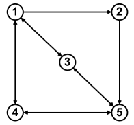
Figure 1: Communication topology graph $\mathcal{G}$.

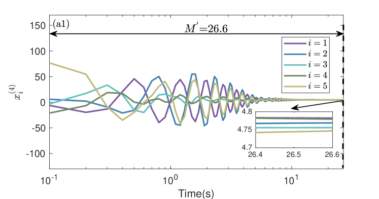
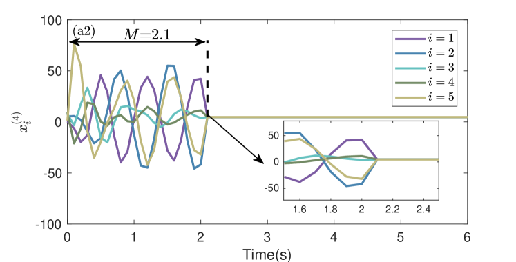
(a) Temporal evolution of $x_{i}^{(4)}$ for routine protocol (a1) and MDCP (a2).

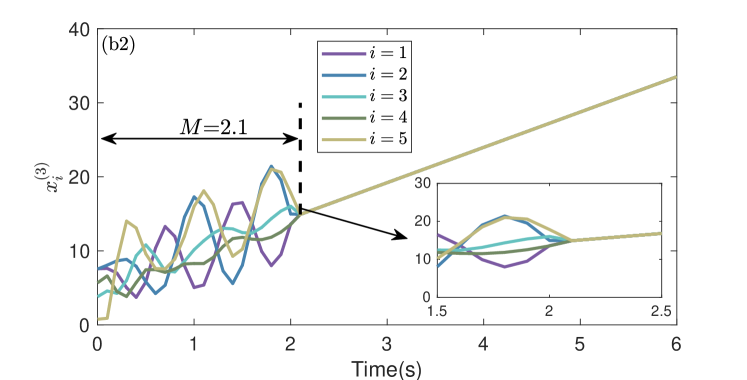
(b) Temporal evolution of $x_{i}^{(3)}$ for routine protocol (b1) and MDCP (b2).

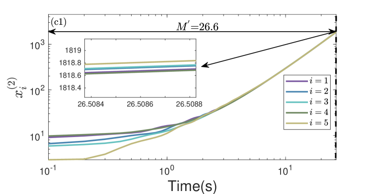
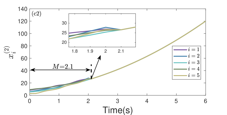
(c) Temporal evolution of $x_{i}^{(2)}$ for routine protocol (c1) and MDCP (c2).

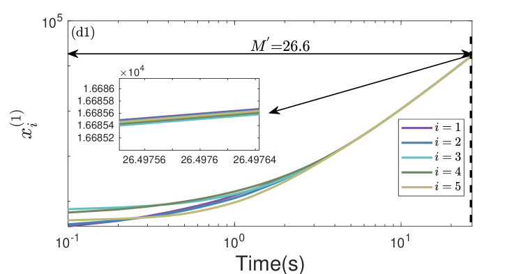
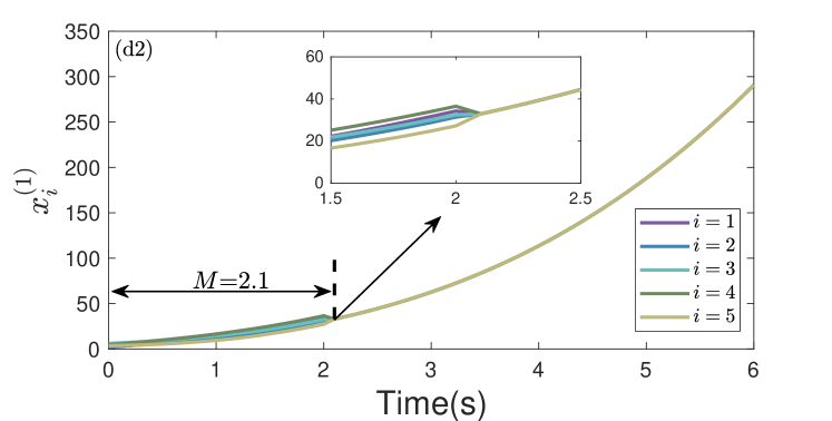
(d) Temporal evolution of $x_{i}^{(1)}$ for routine protocol (d1) and MDCP (d2).

Figure 2: Temporal evolution of state for the fourth-order MAS with topology shown in Fig. 1, the method in (Ren et al., 2007) is adopted as the routine procedure.

Consider a discrete-time 4-order linear MAS composed of five agents governed by (1) and (2), whose communication topology is given in Fig. 1. Pick the external coupling weight $\omega=-0.2$, internal coupling weight $c_{0}=6,c_{1}=6,c_{2}=17,c_{3}=2$, sampling time $\epsilon=0.1$. The Laplacian matrix is given as follows

$$\mathcal{L}=\left[\begin{array}[]{ccccc}2&0&-1&-1&0\\ -1&1&0&0&0\\ -1&0&2&0&-1\\ -1&0&0&2&-1\\ 0&-1&-1&-1&3\end{array}\right].$$

The initial values

$$X(0)=[ 1.9660\quad 2.5108\quad 6.1604\quad 4.7329\quad 3.5166$$

$$8.3083\quad 5.8526\quad 5.4972\quad 9.1719\quad 2.8584$$

$$7.5720\quad 7.5373\quad 3.8045\quad 5.6782\quad 0.7585$$

$$0.5395\quad 5.3080\quad 7.7917\quad 9.3401\quad 1.2991]^{\mbox{\tiny\sf T}}$$

are generated randomly.

According to (4), the corresponding Perron matrix is set as follows

$$W=\left[\begin{array}[]{cccccc}I_{5}&0.1I_{5}&\mathbf{0}_{5}&\mathbf{0}_{5}\\ \mathbf{0}_{5}&I_{5}&0.1I_{5}&\mathbf{0}_{5}\\ \mathbf{0}_{5}&\mathbf{0}_{5}&I_{5}&0.1I_{5}\\ -1.2\mathcal{L}&-1.2\mathcal{L}&-3.4\mathcal{L}&I_{5}-0.4\mathcal{L}\end{array}\right].$$

Consider the first agent, i.e., $i=1$. Establish a Hankel matrix by (22), increase $\widehat{\overline{D}}_{1}$ until $\Gamma$ loses rank. Then, $\widehat{\overline{D}}_{1}=10$, which implies $2\widehat{\overline{D}}_{1}+1=21$ is the minimal individual memory length. Besides, $\Gamma^{\bot}$ is given as follows

$$\zeta_{1}=[ 0.0000,0.7209,-3.2848,7.5597,-10.8951,9.8706,$$

$$-4.0706,-2.6171,5.2873,-3.5668,1.0000]^{\mbox{\tiny\sf T}},$$

which is the coefficient of (19). Together with (18), the minimal polynomial pair of $W$ is calculated below

$$\alpha_{1}=[ 0.0000,0.7209,-6.1685,25.0245,-63.7266,$$

$$112.6697,-142.4475,124.0291,-59.0453,-14.2656,$$

$$53.3886,-49.1670,25.5545,-7.5668,1.0000]^{\mbox{\tiny\sf T}}.$$

Then, (25) can be obtained. According to (28), one has that

$$[\beta_{0},\beta_{1}\dots\beta_{3}]^{\mbox{\tiny\sf T}}=[0.0048\quad 0.0538\quad 0.6762\quad 3.7570]^{\mbox{\tiny\sf T}}.$$

Besides, $b_{3-j}=\beta_{j}\text{ for }j=0,1,\cdots,3$. According to (31), the first-order consensus item of the first agent is computed as $\widetilde{\wp}_{c}^{(1)}(k)=0.000794850061k^{3}+0.02451822315k^{2}+0.6508490022k+3.757019522$. Here, the result is converted from a fraction to decimal with 10 significant figures for convenience. In addition, once the first agent has predicted the eventual consensus value, it will send the value to other ones simultaneously.

To compare the performances of the present MDCP and the routine consensus control protocol for high-order MASs (Ren et al., 2007) (in Abbr. Ren’s protocol), let $M^{{}^{\prime}}$, $M$ denote consensus-window-launch-time (CWLT) of Ren’s protocol and MDCP, respectively, here $\sigma=0.1$. Note that the smaller the $\sigma$ is the larger the CWLT is. As shown in Figs. 2 (a2-d2), deadbeat convergence to the consensus state is achieved by the present MDCP. By contrast, from Figs. 2 (a1-d1), it is observed that Ren’s protocol yields asymptotic convergence to the eventual same consensus value. Thus, the main technical results of Theorem 1 and 2 are verified.

To examine the feasibility of the proposed MDCP on more general complex networks, we consider benchmark Erdös–Rényi ($\mathrm{ER}$) (Erdos et al., 1960), Barabási–Albert ($\mathrm{BA}$) (Barabási & Albert, 1999) and Watts–Strogatz ($\mathrm{BA}$) (Watts & Strogatz, 1998) networks. In the $\mathrm{ER}$ network, node pairs are connected with a probability $\rho$. Initially, $\mathrm{BA}$ networks is a small clique of $m$ nodes, and at each time step, a new node is introduced and connected to $m$ existing nodes. $\mathrm{WS}$ network is a lattice where each node connects to $z$ neighbors with a rewiring probability of $0.3$. We generate $\mathcal{S}=100$ networks of size $N=20$ for each kind of network model randomly with randomly initial individual state in the range $\left[0,30\right]$. In each network, we pick up an observed node $i$ from $20$ nodes independent runs. Define the average CWLT of $\mathcal{S}$ networks with $N$ agents as $\overline{M}=\frac{1}{N\times\mathcal{S}}\sum_{j=1}^{\mathcal{S}}\sum_{i=1}^{N}M_{i,j}\text{ and }\overline{M^{{}^{\prime}}}=\frac{1}{\mathcal{S}}\sum_{j=1}^{\mathcal{S}}M^{{}^{\prime}}_{j}$, respectively. Here, $\sigma=0.1$, $M_{i,j}$ denotes CWLT for the $i$-th agent of the $j$-th networks, and $M^{{}^{\prime}}_{j}$ refers to CWLT of the $j$-th networks. It is observed from Fig. 3 that the average CWLT of MDCP is much shorter than Ren’s protocol ($\mathrm{ER}(\rho=0.2)$: 5.20s VS 54.05s, $\mathrm{ER}(\rho=0.4)$: 4.32s VS 32.26s, $\mathrm{WS}(z=6)$: 6.63s VS 42.88s, $\mathrm{WS}(z=8)$: 6.58s VS 35.94s, $\mathrm{BA}(m=6)$: 4.78s VS 35.87s, $\mathrm{BA}(m=9)$: 4.44s VS 27.24s), which implies that consensus has been substantially accelerated by locally sequential observations. Both the feasibility of Theorems 1 and 2, and the superiority of the present MDCP have thus been verified.

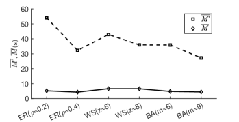
Figure 3: The average CWLT $\overline{M^{{}^{\prime}}}$ and $\overline{M}$ computed for independent $\mathcal{S}=100$ $\mathrm{ER},\mathrm{BA},\mathrm{WS}$ networks with size $N=20$ independently.

5 Conclusion

In this paper, both minimal-time deadbeat consensus and instant individual disagreement degree prediction problems are addressed by the propose MDCP for a class of discrete-time high-order linear MASs with directed communication topological backbones. Deadbeat consensus is achieved to fulfill prompt coordination requirements of modern industrial MASs. Sufficient conditions concerning the topology and the associate eigenspectrum of Perron matrix are derived to guarantee the minimal-time deadbeat consensus and instant individual disagreement degree prediction. Extensive simulations are conducted on a variety of benchmark complex networks to show the effectiveness and superiority of the proposed MDCP protocol. The present MDCP can be expected to pave the way from minimal time deadbeat consensus theory to prompt responses to emergence of natural/social/engineering swarming systems.

This work is supported by the National Natural Science Foundation of China under Grants 62225306 and U2141235.

References

• Attanasi et al. (2014) Attanasi, A., Cavagna, A., Del Castello, L., Giardina, I., Grigera, T. S., Jelić, A., Melillo, S., Parisi, L., Pohl, O., Shen, E. et al. (2014). Information transfer and behavioural inertia in starling flocks. Nature physics, 10, 691–696.
• Barabási & Albert (1999) Barabási, A.-L., & Albert, R. (1999). Emergence of scaling in random networks. science, 286, 509–512.
• Cavagna et al. (2015) Cavagna, A., Del Castello, L., Giardina, I., Grigera, T., Jelic, A., Melillo, S., Mora, T., Parisi, L., Silvestri, E., Viale, M. et al. (2015). Flocking and turning: a new model for self-organized collective motion. Journal of Statistical Physics, 158, 601–627.
• Charalambous & Hadjicostis (2018) Charalambous, T., & Hadjicostis, C. N. (2018). When to stop iterating in digraphs of unknown size? an application to finite-time average consensus. In 2018 European Control Conference (ECC) (pp. 1–7). IEEE.
• Charalambous et al. (2015) Charalambous, T., Yuan, Y., Yang, T., Pan, W., Hadjicostis, C. N., & Johansson, M. (2015). Distributed finite-time average consensus in digraphs in the presence of time delays. IEEE Transactions on Control of Network Systems, 2, 370–381.
• Dimarogonas & Kyriakopoulos (2007) Dimarogonas, D. V., & Kyriakopoulos, K. J. (2007). On the rendezvous problem for multiple nonholonomic agents. IEEE Transactions on Automatic Control, 52, 916–922.
• Erdos et al. (1960) Erdos, P., Rényi, A. et al. (1960). On the evolution of random graphs. Publ. Math. Inst. Hung. Acad. Sci, 5, 17–60.
• Fax & Murray (2004) Fax, J. A., & Murray, R. M. (2004). Information flow and cooperative control of vehicle formations. IEEE Transactions on Automatic Control, 49, 1465–1476.
• Horn & Johnson (2012) Horn, R. A., & Johnson, C. R. (2012). Matrix analysis. Cambridge University Press.
• Hu et al. (2019) Hu, Z., Fu, D., & Zhang, H.-T. (2019). Decentralized finite time consensus for discrete-time high-order linear multi-agent system. In 2019 Chinese Control Conference (CCC) (pp. 6154–6159). IEEE.
• Huang et al. (2014) Huang, J., Fang, H., Dou, L., & Chen, J. (2014). An overview of distributed high-order multi-agent coordination. IEEE/CAA Journal of Automatica Sinica, 1, 1–9.
• Jadbabaie et al. (2003) Jadbabaie, A., Lin, J., & Morse, A. S. (2003). Coordination of groups of mobile autonomous agents using nearest neighbor rules. IEEE Transactions on Automatic Control, 48, 988–1001.
• Liu et al. (2019) Liu, B., Chen, Z., Zhang, H.-T., Wang, X., Geng, T., Su, H., & Zhao, J. (2019). Collective dynamics and control for multiple unmanned surface vessels. IEEE Transactions on Control Systems Technology, 28, 2540–2547.
• Manitara & Hadjicostis (2017) Manitara, N. E., & Hadjicostis, C. N. (2017). Distributed stopping for average consensus in digraphs. IEEE Transactions on Control of Network Systems, 5, 957–967.
• Moreau (2005) Moreau, L. (2005). Stability of multiagent systems with time-dependent communication links. IEEE Transactions on Automatic Control, 50, 169–182.
• Olfati-Saber (2006) Olfati-Saber, R. (2006). Flocking for multi-agent dynamic systems: Algorithms and theory. IEEE Transactions on Automatic Control, 51, 401–420.
• Olfati-Saber & Murray (2004) Olfati-Saber, R., & Murray, R. M. (2004). Consensus problems in networks of agents with switching topology and time-delays. IEEE Transactions on Automatic Control, 49, 1520–1533.
• Olver (1993) Olver, P. J. (1993). Applications of Lie groups to differential equations volume 107. Springer Science & Business Media.
• Partington (1988) Partington, J. R. (1988). An introduction to Hankel operators. 13. Cambridge University Press.
• Proskurnikov et al. (2015) Proskurnikov, A. V., Matveev, A. S., & Cao, M. (2015). Opinion dynamics in social networks with hostile camps: Consensus vs. polarization. IEEE Transactions on Automatic Control, 61, 1524–1536.
• Ren & Beard (2005) Ren, W., & Beard, R. W. (2005). Consensus seeking in multiagent systems under dynamically changing interaction topologies. IEEE Transactions on Automatic Control, 50, 655–661.
• Ren & Beard (2008) Ren, W., & Beard, R. W. (2008). Distributed Consensus in Multi-Vehicle Cooperative Control. Springer.
• Ren et al. (2007) Ren, W., Moore, K. L., & Chen, Y. (2007). High-order and model reference consensus algorithms in cooperative control of multivehicle systems. Journal of Dynamic Systems, Measurement and Control, 129, 678–688.
• Rezaee & Abdollahi (2015) Rezaee, H., & Abdollahi, F. (2015). Average consensus over high-order multiagent systems. IEEE Transactions on Automatic Control, 60, 3047–3052.
• Seo et al. (2009) Seo, J. H., Shim, H., & Back, J. (2009). Consensus of high-order linear systems using dynamic output feedback compensator: Low gain approach. Automatica, 45, 2659–2664.
• Su & Lin (2016) Su, S., & Lin, Z. (2016). Distributed consensus control of multi-agent systems with higher order agent dynamics and dynamically changing directed interaction topologies. IEEE Transactions on Automatic Control, 61, 515–519. doi:10.1109/TAC.2015.2444211.
• Sun et al. (2017) Sun, S., Lin, H., Ma, J., & Li, X. (2017). Multi-sensor distributed fusion estimation with applications in networked systems: A review paper. Information Fusion, 38, 122–134.