Sub-Optimal Moving Horizon Estimation in Feedback Control of Linear Constrained Systems

Abstract

Moving horizon estimation (MHE) offers benefits relative to other estimation approaches by its ability to explicitly handle constraints, but suffers increased computation cost. To help enable MHE on platforms with limited computation power, we propose to solve the optimization problem underlying MHE sub-optimally for a fixed number of optimization iterations per time step. The stability of the closed-loop system is analyzed using the small-gain theorem by considering the closed-loop controlled system, the optimization algorithm dynamics, and the estimation error dynamics as three interconnected subsystems. By assuming incremental input/output-to-state stability ($\delta$-IOSS) of the system and imposing standard ISS conditions on the controller, we derive conditions on the iteration number such that the interconnected system is input-to-state stable (ISS) w.r.t. the external disturbances. A simulation using an MHE-MPC estimator-controller pair is used to validate the results.

I introduction

MHE is an optimization-based method that considers a fixed window of past measurements and the system’s constraints in estimating the current state. Due to the inclusion of the constraints explicitly in the problem formulation, MHE has been shown to produce more accurate state estimates compared to the extended Kalman Filter [1]. Assuming detectability of the system, rather than observability, MHE was shown to posses robust global asymptotic stability w.r.t. bounded disturbances and the estimation error converges in case of bounded and vanishing disturbances [2].

Although MHE offers the benefit of considering constraints, its application is limited by the computational cost, particularly in systems with fast dynamics or platforms with limited computational resources. To alleviate this issue, [3] introduced an auxiliary observer to provide pre-estimation for MHE. However, despite reduced computation time, the iteration number required to solve the MHE problem with stability guarantees cannot be determined offline. In [4], a feasible candidate solution from an auxiliary observer is improved for a limited but varying amount of iterations to obtain a sub-optimal solution so that the resulting estimate is robustly stable. The proximity-MHE scheme in [5] performs limited optimization iterations with a proximity regularizing term to improve the prior estimate from an auxiliary observer and guarantees the nominal stability of the MHE.

Other approaches concentrated on the optimization scheme that underlies the MHE problem. For example, [6] proposed to enforce move blocking on the disturbance sequence in MHE to reduce the associated computation burden, which also guarantees the nominal stability of MHE. In [7], a real-time iteration scheme is applied to MHE without inequality constraints. Local convergence is guaranteed when a single optimization iteration is performed per time step. The work [8] combined this scheme with automatic code generation to obtain highly efficient source code of MHE algorithms. For noise-free systems, [9] solves the MHE problem for single or multiple iterations with gradient-based, conjugate gradient-based, and Newton methods and achieves local stability.

Compared to the aforementioned works, we study the stability of the closed-loop with a sub-optimal MHE and a feedback control law. Earlier studies often treated MHE and the feedback controller as separate modules, with MHE providing estimates with bounded error [10], and the controller designed to ensure stability. Instead, we aim to jointly determine conditions that guarantee stability of both MHE and the controlled system. To achieve this, we employ an stability analysis framework from the sub-optimal model predictive control (MPC) literature [11],[12],[13]. Therein, the closed-loop system was formulated as an interconnection of a controlled system and an optimization algorithm dynamics.

In this paper, we propose a sub-optimal MHE scheme where, at every time step, the MHE problem is warm-started with the previous solution and then solved by an optimization algorithm with a fixed number of iterations. Then, the resulting sub-optimal estimate is used for feedback control of a linear system with state and input constraints.

Our main contribution lies in the stability analysis, which follows a similar approach as [11], [12], and [13]. We first characterize the interaction between the closed-loop controlled system, the sub-optimality error dynamics (of the optimization algorithm used for solving the MHE problem), and the state estimation error dynamics as three interconnected subsystems. Then, assuming the controller is robustly stabilizing, the small-gain theorem is used to derive conditions on the optimization iteration number for guaranteeing the interconnected system is input-to-state stable (ISS) w.r.t to the external disturbances.

Notations: Let $\mathbb{S}_{\succ 0}$ be the set of positive definite matrices. Let $\mathbf{I}^{n}$ be the identity matrix of size $n$. Let $\mathbf{0}^{m\times n}$ be the zero matrix of size $m\times n$. For a vector $x\in\mathbb{R}^{n_{x}}$ and a matrix $U\in\mathbb{S}^{n_{x}\times n_{x}}_{\succ 0}$, let $\|x\|$ and $\|x\|_{U}$ denote the $l_{2}$-norm and the weighted $l_{2}$-norm of $x$, respectively. Consider square matrices $U$ and $V$. Let $\|U\|$ denote the spectral norm. Let $\overline{\lambda}_{U}$ and $\underline{\lambda}_{U}$ denote the largest and smallest eigenvalues of $U$, respectively. Let $\Lambda^{U}_{V}:=\overline{\lambda}(U)/\underline{\lambda}(V)$. Let $\mathbb{I}_{[a,b]}$ denote the set of integers in $[a,b]\in\mathbb{R}$. For a variable $v_{t}\in\mathbb{R}^{n_{v}}$ and time steps $a,b\in\mathbb{I}_{[a,b]}$, let $\mathbf{v}_{[a,b]}:=\{v_{a},\cdots,v_{b}\}$ and $\|\mathbf{v}_{[a,b]}\|:=\sup_{t\in\mathbb{I}_{[a,b]}}\|v_{t}\|$. A continuous function $\gamma:\mathbb{R}_{+}\rightarrow\mathbb{R}_{+}$ is of class $\mathcal{K}$ if it is strictly increasing and $\gamma(0)=0$. If it is also unbounded, then it is of class $\mathcal{K}_{\infty}$. If $\gamma$ is strictly decreasing and $\gamma(s)\rightarrow 0$ as $s\rightarrow 0$, then it is of class $\mathcal{L}$. A continuous function $\beta:\mathbb{R}_{+}\times\mathbb{R}_{+}\rightarrow\mathbb{R}_{+}$ is of class $\mathcal{KL}$ if $\beta(\cdot,s)\in\mathcal{K}$ for each fixed $s$ and $\beta(r,\cdot)\in\mathcal{L}$ for each fixed $r$.

II Controller and MHE Formulation

II-A Dynamic System with State Feedback Controller

Consider a system with linear time-invariant dynamics

$$x_{t+1} =Ax_{t}+Bu_{t}+w^{1}_{t},$$ (1)

$$y_{t} =Cx_{t}+w^{2}_{t},$$

with state $x_{t}\in\mathcal{X}\subset\mathbb{R}^{n_{x}}$, input $u_{t}\in\mathcal{U}\subset\mathbb{R}^{n_{u}}$, output measurement $y_{t}\in\mathcal{Y}\subset\mathbb{R}^{n_{y}}$, external disturbance $w^{1}_{t}\in\mathcal{W}_{1}\subset\mathbb{R}^{n_{x}}$, and measurement noise $w^{2}_{t}\in\mathcal{W}_{2}\subset\mathbb{R}^{n_{y}}$. Let $w_{t}:=[{w^{1}_{t}}^{\top},{w^{2}_{t}}^{\top}]^{\top}\in\mathcal{W}\subset\mathbb{R}^{n_{x+y}}$ be the augmented disturbance. Let $\mathcal{Z}:=\mathcal{X}\times\mathcal{U}\times\mathcal{Y}\times\mathcal{W}$ be the Cartesian product of the constraint sets.

Assumption 1.

$\mathcal{Z}$ is convex and contains the origin.

Assumption 2.

Consider system (1). There exist $P,Q,R\in\mathbb{S}_{\succ 0}$ and $\eta\in[0,1)$ that satisfy

$$\left(\begin{array}[]{cc}A^{\top}PA-\eta P-C^{\top}RC&A^{\top}P\bar{B}-C^{\top}R\bar{D}\\ \bar{B}^{\top}PA-\bar{D}^{\top}RC&\bar{B}^{\top}P\bar{B}-Q-\bar{D}^{\top}R\bar{D}\end{array}\right)\preceq 0,$$ (4)

$$\bar{B}=[\textbf{{I}}^{n_{x}},\textbf{{0}}^{n_{x}\times n_{y}}],\quad\bar{D}=[\textbf{{0}}^{n_{y}\times n_{x}},\textbf{{I}}^{n_{y}},].$$ (5)

From Corollary 3 of [14], we know Assumption 2 implies system (1) admits a $\delta$-IOSS Lyapunov function and is detectable. Specifically, for $(x,u,y,w),(x^{\prime},u,y^{\prime},w^{\prime})\in\mathcal{Z}$, where $y=Cx+w^{2}$ and $y^{\prime}=Cx^{\prime}+{w}^{2}{{}^{\prime}}$, the function

$$W_{\delta}(x,x^{\prime})=\|x-x^{\prime}\|_{P}^{2}$$ (6)

is a $\delta$-IOSS Lyapunov function for system (1), satisfying

$$W_{\delta}(Ax+Bu+w^{1},Ax^{\prime}+Bu+w^{1}{{}^{\prime}})$$

$$\quad\leq\eta W_{\delta}(x,x^{\prime})+\|w-w^{\prime}\|_{Q}^{2}+\|y-y^{\prime}\|_{R}^{2}.$$ (7)

Consider the system (1) with a state feedback controller $u_{t}:=\pi(\hat{x}_{t}):\mathcal{X}\rightarrow\mathcal{U}$ satisfying Assumptions 3 and 4,

$$x_{t+1} =Ax_{t}+B\pi(\hat{x}_{t})+w^{1}_{t},$$ (8)

where $\hat{x}_{t}\in\mathcal{X}$ is a state estimate with estimation error $e_{t}:=\hat{x}_{t}-x_{t}$.

Assumption 3.

There exists a positive constant $L_{\pi}$ such that, for any $x,x^{\prime}\in\mathcal{X}$, $\pi(\cdot)$ satisfies

$$\|\pi(x)-\pi(x^{\prime})\|\leq L_{\pi}\|x-x^{\prime}\|.$$ (9)

Assumption 4.

The closed-loop controlled system in (8) is input-to-state stable (ISS): Given an initial state $x_{t}\in\mathcal{X}$, an input sequence $\mathbf{u}_{[t,t+g]}\in\mathcal{U}\times\cdots\times\mathcal{U}$ generated from applying $\pi(\cdot)$, an estimation error sequence $\mathbf{e}_{[t,t+g]}\in\mathbb{R}^{n_{x}}\times\cdots\times\mathbb{R}^{n_{x}}$, and a disturbance sequence $\mathbf{w}_{[t,t+g]}\in\mathcal{W}\times\cdots\times\mathcal{W}$, there exist $\beta_{1}\in\mathcal{KL}$, and $\gamma_{1,3},\gamma^{w}_{1}\in\mathcal{K}$ such that, for all $g\geq 0$, the resulting state $x_{t+g}\in\mathcal{X}$ and satisfies

$$\|x_{t+g}\|\leq \beta_{1}(\|x_{t}\|,g)+\gamma_{1,3}(\|{\mathbf{e}}_{[t,t+g]}\|)+\gamma^{w}_{1}(\|\mathbf{w}_{[t,t+g]}\|).$$ (10)

II-B Sub-Optimal Moving Horizon Estimation

At time step $t$, we obtain the state estimate $\hat{x}_{t}$ by solving a MHE problem based on a prior estimation $x^{\textup{prior}}_{t-M_{t}}$, past inputs $\mathbf{u}_{[t-M_{t},t-1]}$, and past output measurements $\mathbf{y}_{[t-M_{t},t-1]}$, with estimation horizon $M_{t}:=\min(M,t)$, $M\in\mathbb{I}_{\geq 0}$. The MHE problem $\mathbb{P}_{t}(x^{\textup{prior}}_{t-M_{t}},{\mathbf{u}}_{t},{\mathbf{y}}_{t})$ is formulated as

$$(\hat{\mathbf{x}}^{*}_{t}, \hat{\mathbf{w}}^{*}_{t},\hat{\mathbf{y}}^{*}_{t})=\underset{\hat{\mathbf{x}}_{t},\hat{\mathbf{w}}_{t},\hat{\mathbf{y}}_{t}}{\operatorname{argmin}}\;V_{\operatorname{MHE}}(\hat{x}_{t-M_{t}\mid t},\hat{\mathbf{w}}_{t},\hat{\mathbf{y}}_{t})$$ (11a)

s.t. $$\hat{x}_{i+1\mid t}=A\hat{x}_{i\mid t}+Bu_{i}+\hat{w}^{1}_{i\mid t},\;\;\,i\in\mathbb{I}_{\left[t-M_{t},t-1\right]},$$ (11b)

$$\hat{y}_{i\mid t}=C\hat{x}_{i\mid t}+\hat{w}^{2}_{i\mid t},\;\;\;\;\;\;\;\;\;\;\;\;\;\;\;\;\;i\in\mathbb{I}_{\left[t-M_{t},t-1\right]},$$ (11c)

$$\hat{w}_{i\mid t}\in\mathcal{W},\;\hat{y}_{i\mid t}\in\mathcal{Y},\;\;\;\;\;\;\;\;\;\;\;\;\;\;\;\,\;i\in\mathbb{I}_{\left[t-M_{t},t-1\right]},$$ (11d)

$$\hat{x}_{i\mid t}\in\mathcal{X},\;\;\;\;\;\;\;\;\;\;\;\;\;\;\;\;\;\;\;\;\;\;\;\;\;\;\;\;\;\;\;\;\,i\in\mathbb{I}_{\left[t-M_{t},t\right]},$$ (11e)

where the cost is defined as

$$V_{\operatorname{MHE}}(\hat{x}_{t-{M_{t}}\mid t},\hat{\mathbf{w}}_{t},\hat{\mathbf{y}}_{t}):=2\eta^{M_{t}}W_{\delta}(\hat{x}_{t-{M_{t}}\mid t},x^{\textup{prior}}_{t-{M_{t}}})$$

$$\;\;+\sum_{i=1}^{M_{t}}\eta^{i-1}\left(2\left\|\hat{w}_{t-i\mid t}\right\|_{Q}^{2}+\left\|\hat{y}_{t-i\mid t}-y_{t-i}\right\|_{R}^{2}\right),$$ (12)

with $\eta$, $P$, $Q$, and $R$ satisfying (4). The decision variables $\hat{\mathbf{x}}_{t}:=\{\hat{x}_{t-M_{t}\mid t},\cdots,\hat{x}_{t\mid t}\}$, $\hat{\mathbf{w}}_{t}:=\{\hat{w}_{t-M_{t}\mid t},\cdots,\hat{w}_{t-1\mid t}\}$, and $\hat{\mathbf{y}}_{t}:=\{\hat{y}_{t-M_{t}\mid t},\cdots,\hat{y}_{t-1\mid t}\}$ denote the estimated states, augmented disturbances, and measurements, respectively. The cost functions (II-B) can be reformulated as

$$V_{\operatorname{MHE}}(\hat{x}_{t-M_{t}\mid t},\hat{\mathbf{w}}_{t},\hat{\mathbf{y}}_{t}):=\|z_{t}-\tilde{z}_{t}\|^{2}_{H_{t}},$$ (13)

where

$$z_{t}:= [{\hat{x}_{t-{M_{t}}\mid t}}^{\top},{\hat{{w}}_{t-M_{t}\mid t}}^{\top},{\hat{{y}}_{t-M_{t}\mid t}}^{\top},\cdots,{\hat{{w}}_{t-1\mid t}}^{\top},\hat{y}_{t-1\mid t}^{\top}]^{\top},$$ (14)

$$\tilde{z}_{t}:= [x^{\textup{prior}\top}_{t-{M_{t}}},{\mathbf{0}^{n_{w}}}^{\top},y_{t-M_{t}}^{\top},\cdots,{\mathbf{0}^{n_{w}}}^{\top},y_{t-1}^{\top}]^{\top},$$

$$H_{t}:= \operatorname{blkdiag}(2\eta^{M_{t}}P,2\eta^{M_{t}-1}Q,\eta^{M_{t}-1}R,\cdots,2Q,R).$$

Given $\mathbf{u}_{t}$, the state sequence $\hat{\mathbf{x}}_{t}$ can be constructed from $z_{t}$. Let $(\hat{\mathbf{x}}^{*}_{t},\hat{\mathbf{y}}^{*}_{t},\hat{\mathbf{w}}^{*}_{t})$ and $z^{*}_{t}$ denote the optimal solution to (11), considering the formulations in (9) and (10), respectively. To solve $\mathbb{P}_{t}(x^{\textup{prior}}_{t-M_{t}},{\mathbf{u}}_{t},{\mathbf{y}}_{t})$, we consider optimization algorithms that satisfies Assumption 5.

Assumption 5.

$\mathbb{P}_{t}(x^{\textup{prior}}_{t-M_{t}},{\mathbf{u}}_{t},{\mathbf{y}}_{t})$ is solved by an optimization algorithm whose iteration can be described by a nonlinear mapping $z^{k+1}_{t}=\Phi(z^{k}_{t},\tilde{z}_{t})$, where $k\geq 0$ is the iteration number. Furthermore, given an initial solution $z^{0}_{t}$, the $K_{\textup{th}}$-iteration solution $z^{K}_{t}$ obtained from applying $\Phi(\cdot)$ for $K$ times is feasible, i.e., satisfying (8b)-(8e), and satisfies

$$\|z^{K}_{t}-z^{*}_{t}\|\leq\phi(K)\|z^{0}_{t}-z^{*}_{t}\|,$$ (15)

where $\phi(K)\in(0,1)\forall K>0$ and $\phi\in\mathcal{L}$.

Let $(\hat{\mathbf{x}}^{K}_{t},\hat{\mathbf{y}}^{K}_{t},\hat{\mathbf{w}}^{K}_{t})$ and $z^{K}_{t}$ denote the sub-optimal solution to (11) and define the sub-optimality error as $\epsilon_{t}:=\|z^{K}_{t}-z^{*}_{t}\|$.

III Sub-Optimal MHE-Based Feedback Control

In this section, we introduce a sub-optimal MHE scheme. We characterize the closed-loop system controlled with the proposed scheme as three interconnected subsystems and show each subsystem is ISS. Lastly, we derive conditions on the optimization iteration number that guarantee the interconnected system is ISS w.r.t. the augmented disturbance ${w}_{t}$, through the small-gain theorem. We present the proofs of Propositions 1-3 in the Appendix.

III-A The Sub-Optimal MHE Scheme

Alg. 1 introduces the proposed sub-optimal MHE scheme, employing a warm-start strategy. When $t<M$, the formulation in (11) represents the full information estimator, which grows in size as more information is obtained. Due to this, the solution $z^{K}_{t}$ of $\mathbb{P}_{t}(x^{\textup{prior}}_{t-M_{t}},{\mathbf{u}}_{t},{\mathbf{y}}_{t})$ has a lower dimension compared to the solution $z^{K}_{t+1}$ of $\mathbb{P}_{t+1}(x^{\textup{prior}}_{t-M_{t}+1},{\mathbf{u}}_{t+1},{\mathbf{y}}_{t+1})$ when $t<M$. To ensure the warm-starting step can be smoothly carried out for time steps $t<M$, we use the matrix

$$\Sigma_{t}:=\left\{\begin{array}[]{l}\operatorname{blkdiag}(\mathbf{I}^{n_{z_{t}}-n_{x}-n_{y}},\mathbf{0}^{n_{x}+n_{y}}),\;t<M,\\ \mathbf{I}^{n_{z_{t}}},\quad\quad\quad\quad\quad\quad\quad\quad\quad\quad\;\;\,\;t\geq M,\end{array}\right.$$ (18)

in Step 2 to map $z^{K}_{t}$ to $\Sigma_{t}z^{K}_{t}$, which has the same dimension as $z^{K}_{t+1}$. In Step 3, the operator $\Upsilon({\mathbf{y}}_{t},y_{t})$ appends $y_{t}$ to the end of the sequence ${\mathbf{y}}_{t}$ for all $t\geq 0$, and discards the first element $y_{t-M_{t}}$ in $\mathbf{y}_{t}$ if $t>M$.

Require: $K$, $M$, $\Phi(\cdot)$, $z^{0}_{0}$, $x^{\textup{prior}}_{0}$, ${\mathbf{u}}_{0}$, ${\mathbf{y}}_{0}$;
For $t=0,1,2,\cdots$ Do
1. Obtain $\hat{x}^{K}_{t}$ by solving $\mathbb{P}_{t}(x^{\textup{prior}}_{t-M_{t}},{\mathbf{u}}_{t},{\mathbf{y}}_{t})$ for $K$ iterations using optimization algorithm $\Phi(\cdot)$ with initial solution $z^{0}_{t}$;
2. Warm-starting: $z^{0}_{t+1}\leftarrow\Sigma_{t}z^{K}_{t}$;
3. Update problem parameters: $x^{\textup{prior}}_{t-M_{t}}\leftarrow\hat{x}^{K}_{t-M_{t}\mid t}$, ${\mathbf{u}}_{t+1}\leftarrow\Upsilon({\mathbf{u}}_{t},\pi(\hat{x}^{K}_{t}))$, ${\mathbf{y}}_{t+1}\leftarrow\Upsilon({\mathbf{y}}_{t},y_{t})$;
4. Apply $\pi(\hat{x}^{K}_{t})$ to the system (8);
End

Algorithm 1 Sub-Optimal MHE in Feedback Control

III-B Interconnection of Three Subsystems

We identify three dynamic subsystems from Alg. 1:

Subsys. 1:

Subsys. 2:

Subsys. 3:

They describe the closed-loop controlled system (Subsys. 1), the sub-optimality error dynamics (Subsys. 2), and the estimation error dynamics (Subsys. 3), respectively. Fig. 1 illustrates the interconnections between the three subsystems.

In subsystem 1, the controller $\pi(x_{t})$ attempts to drive $x_{t}$ to the origin. However, $\pi(x_{t})$ is perturbed to $\pi(\hat{x}^{K}_{t\mid t})$ by $e_{t}$. In subsystem 2, $\mathbb{P}_{t}(x^{\textup{prior}}_{t-M_{t}},{\mathbf{u}}_{t},{\mathbf{y}}_{t})$ is solved for $K$ iterations with warm-starting to reduce the sub-optimality error (drive $z^{0}_{t}=\Sigma_{t-1}z^{K}_{t-1}$ to $z^{*}_{t}$). The optimal solution $z^{*}_{t}$ can be seen as a perturbed solution of $z^{*}_{t-1}$, resulting from the problem parameter update in Step 3 of Alg. 1. In subsystem 3, the MHE attempts to drive the estimation error to zero. This process is disturbed by the change in state $x_{t}$ and the sub-optimality error $\epsilon_{t}$. The stability of the interconnected system (19) can be analyzed via the small-gain theorem, which requires each subsystem to be ISS. Note that subsystem 1 in (19c) already meets this requirement via Assumption 4.

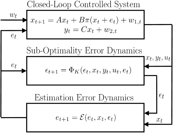
Figure 1: The interconnection of three subsystems.

III-C ISS of the Sub-Optimality Error Dynamics (Subsystem 2)

To prove the sub-optimality error dynamics is ISS, we first show the difference between two consecutive optimal solutions $z^{*}_{t-1}$ and $z^{*}_{t}$ is bounded w.r.t. the changes in the parameters of $\mathbb{P}_{t}(x^{\textup{prior}}_{t-M_{t}},{\mathbf{u}}_{t},{\mathbf{y}}_{t})$.

Lemma 1.

Suppose Assumptions 1-2 hold. Then, there exists a Lipschitz constant $L_{\Phi}>1$ such that the optimal solutions of $\mathbb{P}_{t-1}(x^{\textup{prior}}_{t-M_{t}-1},{\mathbf{u}}_{t-1},{\mathbf{y}}_{t-1})$ and $\mathbb{P}_{t}(x^{\textup{prior}}_{t-M_{t}},{\mathbf{u}}_{t},{\mathbf{y}}_{t})$ satisfy

$$\|\Sigma_{t-1}z^{*}_{t-1}-z^{*}_{t}\|\leq L_{\Phi}(\|\tilde{z}_{t-1}-\Sigma^{\top}_{t-1}\tilde{z}_{t}\|+\sigma_{t}),$$ (20)

with $\tilde{z}_{t}$ and $\tilde{z}_{t-1}$ defined in (14), $\Sigma_{t}$ defined in (18), and

$$\sigma_{t}:=\left\{\begin{array}[]{l}(1-\eta^{-1})\|H_{t}\|+\|A\|+\|B\|+\|C\|+2,\,t\leq M,\\ 0,\quad\quad\quad\quad\quad\quad\quad\quad\quad\quad\quad\quad\quad\quad\quad\quad\;\,\,t>M.\end{array}\right.$$ (23)

Proof.

We prove (20) by treating $\mathbb{P}_{t}(\cdot)$ as a parametric optimization problem, whose cost function is strongly convex (from Assumption 2), inequality constraints are convex, and equality constraints are affine. For $t>M$, using Theorem 3.1 in [15] and the fact $\Sigma_{t}=\mathbf{I}^{n_{z_{t}}}$ for $t\geq M$ from (18), we know there exists a Lipschitz constant $L_{\Phi}>1$ such that

$$\|\Sigma_{t-1}z^{*}_{t-1}-z^{*}_{t}\|\leq L_{\Phi}\|\tilde{z}_{t-1}-\Sigma^{\top}_{t-1}\tilde{z}_{t}\|.$$ (24)

For $t\leq M$, we consider an equivalent expression of $\mathbb{P}_{t}(\hat{x}_{0},{\mathbf{u}}_{t},{\mathbf{y}}_{t})$, given by $\mathbb{P}_{t}^{\prime}(\hat{x}_{0},\allowbreak{\mathbf{u}}_{t},\allowbreak{\mathbf{y}}_{t},H_{t},\allowbreak A,\allowbreak B,\allowbreak\mathbf{I}^{n_{x}},C,\mathbf{I}^{n_{y}})$. The matrix $H_{t}$ is from the cost (13). The last five matrices are from the system constraints (11b) and (11c), $i\allowbreak=\allowbreak t-1$, respectively. Let $\check{\mathbb{P}}_{t}:=\mathbb{P}_{t}^{\prime}(\hat{x}_{0},\allowbreak{\mathbf{u}}_{t},\allowbreak{\mathbf{y}}_{t},\allowbreak\eta^{-1}H_{t},\allowbreak\mathbf{0}^{n_{x}},\allowbreak\mathbf{0}^{n_{x}\times n_{u}},\allowbreak\mathbf{0}^{n_{x}},\allowbreak\mathbf{0}^{n_{y}\times n_{u}},\allowbreak\mathbf{0}^{n_{y}})$, with optimal solution $\check{z}^{*}_{t}$. With $A,\allowbreak B,\allowbreak\mathbf{I}^{n_{x}},C,\mathbf{I}^{n_{y}}=\mathbf{0}$, $\check{\mathbb{P}}_{t}$ is equivalent to $\mathbb{P}_{t-1}(\hat{x}_{0},{\mathbf{u}}_{t-1},{\mathbf{y}}_{t-1})$ with inactive system constraints at $i=t-1$. Thus, $\check{z}^{*}_{t}=\Sigma_{t-1}z^{*}_{t-1}$. Similar to (24), we know there exists $L_{\Phi}>1$ such that the optimal solutions of $\check{z}^{*}_{t}$ and $z^{*}_{t-1}$ satisfy

$$\|\check{z}^{*}_{t}-z^{*}_{t}\|\leq L_{\Phi}\sigma_{t}\Rightarrow\|\Sigma_{t-1}z^{*}_{t-1}-z^{*}_{t}\|\leq L_{\Phi}\sigma_{t}.$$ (25)

Since $\|\tilde{z}_{t-1}-\Sigma^{\top}_{t-1}\tilde{z}_{t}\|=0$ for $t\leq M$ and $\sigma_{t}=0$ for $t>M$, we can combine (24) and (25) to obtain (20). 0.0pt0.55em0.55em

With the bound in (20), we can show the sub-optimality error dynamics defined in (19d) is ISS:

Proposition 1.

Consider $\mathbb{P}_{t}(x^{\textup{prior}}_{t-M_{t}},{\mathbf{u}}_{t},{\mathbf{y}}_{t})$ solved by an optimization algorithm $\Phi(\cdot)$ for $K$ iterations. Suppose Assumptions 1-5 hold. For $t\geq 0$, the sub-optimality error $\epsilon_{t}$ satisfies

$$\|\epsilon_{t}\|{\leq}\beta_{2}(\|\epsilon_{0}\|,t)+\gamma_{2,1}(\|\mathbf{x}_{[0,t-1]}\|)+\gamma_{2,3}(\|\mathbf{e}_{[0,t-1]}\|)$$

$$\quad\quad\;+\gamma^{w}_{2}(\|\mathbf{w}_{[0,t-1]}\|)+\gamma^{\sigma}_{2}(\|\bm{\sigma}_{[0,t-1]}\|),$$ (26)

where $\beta_{2}(s,t):=\phi(K)^{t}s$, $\gamma_{2,1}(s):=C_{1}(K)/{(1-\phi(K))}s$, $\gamma_{2,3}(s):=C_{2}(K)/{(1-\phi(K))}s$, $\gamma_{2}^{w}(s):=C_{3}(K)/{(1-\phi(K))}s$, and $\gamma_{3}^{\sigma}(s):=\phi(K)L_{\Phi}/{(1-\phi(K))}s$, with $C_{1}(K)$, $C_{2}(K)$, and $C_{3}(K)$ defined in (32)-(34).

III-D ISS of the Estimation Error Dynamics (Subsystem 3)

Inspired by [14], we first construct an $M$-step Lyapunov function for (19e) based on $W_{\delta}(\cdot)$ defined in (6).

Proposition 2.

Suppose Assumptions 1-5 hold. Let $\bar{H}:=\sup_{t\geq 0}(\overline{\lambda}(H_{t}))$. For $t\geq 0$, the state estimate $\hat{x}^{K}_{t\mid t}$ satisfies

$$W_{\delta}(\hat{x}^{K}_{t\mid t},x_{t})\leq 6\eta^{M_{t}}W_{\delta}(\hat{x}^{K}_{t-M_{t}\mid t-M_{t}},x_{t-M_{t}})\allowdisplaybreaks$$

$$\quad\quad\quad+2\bar{H}\|\epsilon_{t}\|^{2}+6\sum_{j=1}^{M_{t}}\eta^{j-1}\|w_{t-j}\|^{2}_{Q}.$$ (27)

Based on the $M$-step Lyapunov function in (2), we show the estimation error dynamics is ISS.

Proposition 3.

Suppose Assumptions 1-5 hold. Then, the estimation error dynamics is ISS and $\hat{x}^{K}_{t\mid t}$ satisfies

$$\|e_{t}\|\leq \beta_{3}(\|e_{0}\|,t)+\gamma_{3,1}(\|\mathbf{x}_{[0,t-1]}\|)+\gamma_{3,2}(\|\bm{\epsilon}_{[0,t-1]}\|)$$

$$+\gamma^{w}_{3}(\|\mathbf{w}_{[0,t-1]}\|)+\gamma^{\sigma}_{3}(\|\bm{\sigma}_{[0,t-1]}\|),$$ (28)

where $\beta_{3}(s,t):=C_{e}(K)\sqrt{\rho}^{t}s$, $\gamma_{3,1}(s):=\sqrt{2\Lambda^{\bar{H}}_{P}}C_{1}(K)s$, $\gamma_{3,2}(s):=C_{\epsilon}(K)s$, $\gamma_{3}^{w}(s):=C_{w}(K)s$, and $\gamma_{3}^{\sigma}(s):=\sqrt{2\Lambda^{\bar{H}}_{P}}\phi(K)L_{\Phi}s$, with $\rho$ satisfying $\rho^{M}=6\eta^{M}$ and $C_{e}(K)$, $C_{w}(K)$, and $C_{\epsilon}(K)$ defined in (35)-(37).

III-E Stability of the Interconnected System

Given that subsystems 1, 2, and 3 are ISS satisfying (10), (1), and (3), respectively, we can establish conditions on the iteration number $K$ such that the small-gain theorem is satisfied and the interconnected system is ISS.

Theorem 1.

Consider the interconnected system (19). Suppose Assumptions 1-5 hold. Then, for any $K$ satisfying

$$\gamma_{1,3}\circ\gamma_{3,1}(s)<s,$$ (29)

$$\gamma_{2,3}\circ\gamma_{3,2}(s)<s,$$ (30)

$$\gamma_{1,3}\circ\gamma_{3,2}\circ\gamma_{2,1}(s)<s,$$ (31)

for all $s>0$, the interconnected system (19) is ISS w.r.t. the augmented disturbance $w_{t}$ and virtual disturbance $\sigma_{t}$.

Remark 1.

Since $\gamma_{1,2},\gamma_{1,3},\gamma_{2,1},\gamma_{2,3},\gamma_{3,1},\gamma_{3,2}\in\mathcal{K}$, and $\gamma_{2,1},\gamma_{2,3},\gamma_{3,1}\rightarrow 0$ as $K\rightarrow\infty$, there always exists a iteration number ${K}$ such that (29)-(31) are satisfied.

IV Case study with an MHE-MPC

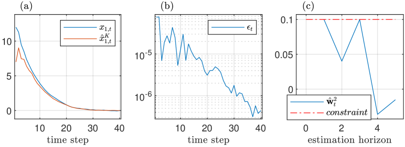
Figure 2: (a) True state vs. Sub-optimal estimate; (b) Change in sub-optimality error; (c) The estimated measurement noise obtained from solving the MHE problem at $t=6$.

To demonstrate Alg. 1 and the theoretical findings, we consider the discrete-time linear system and the corresponding MPC controller in the case study of [11]. We add an output matrix $C=[0.1,0.3,0.8,0.5]$ to the system such that the system is observable. The state $x\in\mathbb{R}^{4}$ and measurement $y\in\mathbb{R}$ are unconstrained, and the input $u\in[-1,1]\times[-1,1]$. Each element of the disturbance vector $w_{t}$ is sampled independently and uniformly from $[-0.1,0.1]$. We found $\gamma_{1,3}(s):=28.8s$, through the method used in Proposition 2 of [16], and $L_{\pi}=2.65$, through a sample-based method.

The parameters of the MHE problem in (11) are $M=5$, $Q=\textbf{I}^{4}$, $R=1$, and $\eta=0.8$, with $P$ computed to satisfy (4). Problem (11) is written in a condensed form and solved using the partial gradient method [11] with convergence rate $\|z^{K}_{t}-z^{*}_{t}\|\leq 0.98^{K}\|z^{0}_{t}-z^{*}_{t}\|$. Accordingly, we define $\phi(K):=0.98^{K}$. The Lipschitz constant $L_{\Phi}=5.32$ is determined through a sample-based method. Finally, the iteration number $K=652$ is computed, which satisfies (29)-(31) with the previously defined parameters.

Given an initial state $x_{0}=[12,-10,10,-10]^{\top}$, $z^{0}_{0}=x^{\textup{prior}}_{0}=[7,-7,3,-5]^{\top}$, and empty sequences $\textbf{y}_{0}$ and $\textbf{u}_{0}$, Alg. 1 is applied for 40 time steps. Fig. 2(a) shows the state $x_{1,t}$ converges asymptotically to a neighbourhood of $0$ and the sub-optimal estimate $\hat{x}^{K}_{1,t}$ converges asymptotically to a neighbourhood of $x_{1,t}$. Fig. 2(b) shows that the sub-optimality error $\epsilon_{t}$ converges asymptotically to a neighbourhood of $0$. Thus, subsystems 1-3 defined in (19c)-(19e) are ISS. Fig. 2(c) shows the estimated measurement noise sequence $\hat{\mathbf{w}}^{2,K}_{t}$ obtained from solving (11) at time step $t=6$, which respects the constraint (in red) by the design of MHE.

V Conclusion

In this work, we proposed a sub-optimal MHE scheme applied to the control of linear systems with constraints. By characterizing Alg. 1 as three interconnected subsystems, we derived conditions on the optimization iteration number for guaranteeing ISS of the interconnected system w.r.t. to external disturbance and measurement noises. A possible extension is to consider the stability of systems controlled by sub-optimal MPC combined with sub-optimal MHE in applications with limited computation resources.

VI Appendix

We define some terms here for clarity:

$$C_{1}(K):=2\phi(K)L_{\Phi}(1+M(\|C\|+L_{\pi}))\allowdisplaybreaks$$ (32)

$$C_{2}(K):=2\phi(K)L_{\Phi}(1+ML_{\pi})\allowdisplaybreaks$$ (33)

$$C_{3}(K):=2\phi(K)L_{\Phi}M\allowdisplaybreaks$$ (34)

$$C_{e}(K):=2\sqrt{3\Lambda^{P}_{P}\Lambda^{\bar{H}}_{P}}\phi(K)L_{\Phi}(\sqrt{\rho}^{-M}+L_{\pi}{\sqrt{\rho}^{-1}})\allowdisplaybreaks$$

$$\quad\;\;+4\sqrt{3\Lambda^{P}_{P}\Lambda^{\bar{H}}_{P}}\phi(K)L_{\Phi}L_{\pi}\sum^{M-1}_{i=1}{\sqrt{\rho}^{-1-i}}+\sqrt{6\Lambda^{P}_{P}}\allowdisplaybreaks$$

$$\quad\;\;+2\sqrt{3\Lambda^{P}_{P}\Lambda^{\bar{H}}_{P}}\phi(K)L_{\Phi}(L_{\pi}+1){\sqrt{\rho}^{-M-1}},\allowdisplaybreaks$$ (35)

$$C_{w}(K):=\sqrt{2\Lambda^{\bar{H}}_{P}}C_{3}(K)+\sqrt{6\Lambda^{Q}_{P}}({1-\sqrt{\rho}})^{-1}\allowdisplaybreaks$$

$$\quad\;\;+4\sqrt{3\Lambda^{\bar{H}}_{P}\Lambda^{Q}_{P}}\phi(K)L_{\Phi}\left(L_{\pi}M+1\right)({1-\sqrt{\rho}})^{-1},\allowdisplaybreaks$$ (36)

$$C_{\epsilon}(K):=\sqrt{2\Lambda^{\bar{H}}_{P}}\phi(K)+\sqrt{2\Lambda^{\bar{H}}_{P}}({1-\sqrt{\rho^{M}}})^{-1}\allowdisplaybreaks$$

$$\quad\;\;+4\Lambda^{\bar{H}}_{P}\phi(K)L_{\Phi}\left(L_{\pi}M+1\right)({1-\sqrt{\rho^{M}}})^{-1}.$$ (37)

Proof of Proposition 1: We break the proof into two cases.

Case 1: For $t\leq M$, due to the warm-start step (Step 2) in Alg. 1, we have

$$\|z^{0}_{t}-z^{*}_{t}\|=\|\Sigma_{t-1}z^{K}_{t-1}-z^{*}_{t}\|$$ (38)

$$\leq\|\Sigma_{t-1}z^{K}_{t-1}-\Sigma_{t-1}z^{*}_{t-1}\|+\|\Sigma_{t-1}z^{*}_{t-1}-z^{*}_{t}\|$$ (39)

$$\overset{\eqref{MHE lipschitz 1}}{\leq}\|\Sigma_{t-1}\|\|z^{K}_{t-1}-z^{*}_{t-1}\|+L_{\Phi}\sigma_{t}.$$ (40)

By multiplying $\phi(K)$ on both sides of the above inequality, and using (15) and the fact $\|\Sigma_{t}\|=1\forall t\in\mathbb{R}$, we have

$$\|\epsilon_{t}\|{\leq}\phi(K)\|\epsilon_{t-1}\|+\phi(K)L_{\Phi}\|\bm{\sigma}_{[0,t-1]}\|.$$ (41)

where we bounded $\sigma_{t}$ with $\|\bm{\sigma}_{[0,t-1]}\|$.

Case 2: For $t>M$, due to the warm-start step (Step 2) in Alg. 1, and $\Sigma^{\top}_{t}=\textbf{I}^{n_{z_{t}}}$ and $\sigma_{t}=0$ for $t>M$, we have

$$\|z^{0}_{t}-z^{*}_{t}\|\leq\|z^{K}_{t-1}-z^{*}_{t-1}\|+\|z^{*}_{t-1}-z^{*}_{t}\|$$ (42)

$$\overset{\eqref{MHE lipschitz 1}}{\leq}\|z^{K}_{t-1}-z^{*}_{t-1}\|+L_{\Phi}\|\tilde{z}_{t-1}-\tilde{z}_{t}\|$$ (43)

$$\leq L_{\Phi}\sum^{M_{t}-1}_{i=0}(\|{u}_{t-1-i}-{u}_{t-2-i}\|+\|{y}_{t-1-i}-{y}_{t-2-i}\|)$$

$$+L_{\Phi}\|\hat{x}^{K}_{t-M\mid t-M}-\hat{x}^{K}_{t-M-1\mid t-M-1}\|+\|\epsilon_{t-1}\|,$$ (44)

where we used $x^{\textup{prior}}_{t-M}=\hat{x}^{K}_{t-M\mid t-M}$ and $x^{\textup{prior}}_{t-M-1}=\hat{x}^{K}_{t-M-1\mid t-M-1}$ in (44). Given the above inequality, we can bound $\|\hat{x}^{K}_{t-M\mid t-M}-\hat{x}^{K}_{t-M-1\mid t-M-1}\|$ with

$$\|\hat{x}^{K}_{t-M\mid t-M}-\hat{x}^{K}_{t-M-1\mid t-M-1}\|$$

$$= \|({x}_{t-M}+{e}_{t-M})-({x}_{t-M-1}+{e}_{t-M-1})\|$$ (45)

$$\leq \|{x}_{t-M_{t}}\|+\|{x}_{t-M_{t}-1}\|+\|{e}_{t-M_{t}}\|+\|{e}_{t-M_{t}-1}\|,$$ (46)

bound $\|{u}_{t-1-i}-{u}_{t-2-i}\|$ with

$$\|{u}_{t-1-i}-{u}_{t-2-i}\|\overset{\eqref{controller lip constant}}{\leq}L_{\pi}\|\hat{x}^{K}_{t-1-i}-\hat{x}^{K}_{t-2-i}\|$$

(47)

and bound $\|{y}_{t-1-i}-{y}_{t-2-i}\|$ with

$$\|{y}_{t-1-i}-{y}_{t-2-i}\|\leq\|{w}_{t-1-i}\|+\|{w}_{t-2-i}\|\allowdisplaybreaks$$

$$+\|C\|\|{x}_{t-1-i}\|+\|C\|\|{x}_{t-2-i}\|.$$ (48)

Using the resulting bound to replace the term $\|z^{0}_{t}-z^{*}_{t}\|$ on the r.h.s. of (15), we have that

$$\|\epsilon_{t}\|\leq\phi(K)\|\epsilon_{t-1}\|+C_{1}(K)\|\mathbf{x}_{[0,t-1]}\|+C_{3}(K)\|\mathbf{w}_{[0,t-1]}\|\allowdisplaybreaks$$

$$+\phi(K)L_{\Phi}\left(\|{e}_{t-M}\|+\|{e}_{t-M-1}\|\right)\allowdisplaybreaks$$

$$+\phi(K)L_{\Phi}\sum^{M-1}_{i=0}\left(L_{\pi}(\|{e}_{t-1-i}\|+\|{e}_{t-2-i}\|)\right).$$ (49)

where the $\|x_{t}\|$ and $\|w_{t}\|$ terms are bounded with $\|\mathbf{x}_{[0,t-1]}\|$ and $\|\mathbf{w}_{[0,t-1]}\|$, respectively. Next, bounding the $\|e_{t}\|$ terms in (49) with $\|\mathbf{e}_{[0,t-1]}\|$ gives

$$\|\epsilon_{t}\|{\leq}\phi(K)\|\epsilon_{t-1}\|+C_{1}(K)\|\mathbf{x}_{[0,t-1]}\|$$

$$\quad+C_{2}(K)\|\mathbf{e}_{[0,t-1]}\|+C_{3}(K)\|\mathbf{w}_{[0,t-1]}\|.$$ (50)

Combining the r.h.s. of (41) and (50) gives

$$\|\epsilon_{t}\|{\leq}\phi(K)\|\epsilon_{t-1}\|+C_{1}(K)\|\mathbf{x}_{[0,t-1]}\|+C_{2}(K)\|\mathbf{e}_{[0,t-1]}\|$$

$$\quad+C_{3}(K)\|\mathbf{w}_{[0,t-1]}\|+\phi(K)L_{\Phi}\|\bm{\sigma}_{[0,t-1]}\|,$$ (51)

which holds for all time steps $t>0$. Finally, applying (51) for $t$ times and using the geometric series to simplify $\sum_{i=0}^{t-1}\phi(K)^{(t-1-i)}$ as $1/(1-\phi(K))$ yield (1). 0.55em0.55em

Proof of Proposition 2: We first derive an intermediate bound on $W_{\delta}(\hat{x}^{K}_{t\mid t},x_{t})$. Due to Assumption 5, the sub-optimal solution $(\hat{\mathbf{x}}^{K}_{t},\hat{\mathbf{y}}^{K}_{t},\hat{\mathbf{w}}^{K}_{t})$ is feasible for (11) and forms a feasible trajectory of the system in (1). Given the actual trajectory $({\mathbf{x}}_{[t-M,t]},{\mathbf{y}}_{[t-M,t-1]},{\mathbf{w}}_{[t-M,t-1]})$, we can apply the bound in (II-A) for $M_{t}$ times to obtain

(52)

(53)

(54)

where (53) is obtained by applying the triangle inequality to $W_{\delta}(\hat{x}^{K}_{t-M_{t}\mid t},x_{t-M_{t}})$ and $\|\hat{w}^{K}_{t-j\mid t}-w_{t-j}\|^{2}_{Q}$. Next, we derive a bound on $V_{\textup{MHE}}(\hat{x}^{K}_{t-M_{t}\mid t},\hat{\mathbf{y}}^{K}_{t},\hat{\mathbf{w}}^{K}_{t})$. We know that

$$V_{\textup{MHE}}(\hat{x}^{K}_{t-M_{t}\mid t},\hat{\mathbf{y}}^{K}_{t},\hat{\mathbf{w}}^{K}_{t})=\|z^{K}_{t}-\tilde{z}_{t}\|^{2}_{H_{t}}$$ (55)

$$\leq 2\|z^{K}_{t}-z^{*}_{t}\|^{2}_{H_{t}}+2\|z^{*}_{t}-\tilde{z}_{t}\|^{2}_{H_{t}}$$ (56)

$$\leq 2\|z^{K}_{t}-z^{*}_{t}\|^{2}_{H_{t}}+2V_{\textup{MHE}}(\hat{x}^{*}_{t-M_{t}\mid t},\hat{\mathbf{y}}^{*}_{t},\hat{\mathbf{w}}^{*}_{t})$$ (57)

$$\leq\scalebox{0.99}{$2\|\epsilon_{t}\|^{2}_{H_{t}}+2V_{\textup{MHE}}({{x}}_{t-M_{t}},{\mathbf{y}}_{[t-M_{t},t-1]},{\mathbf{w}}_{[t-M_{t},t-1]})$}$$ (58)

where (58) holds since $({\mathbf{x}}_{[t-M_{t},t]},{\mathbf{y}}_{[t-M_{t},t-1]},{\mathbf{w}}_{[t-M_{t},t-1]})$ forms a sub-optimal solution to (11). Using the above bound with (54) and then using (II-B) give

$$+2V_{\textup{MHE}}({x}_{t-M_{t}},{\mathbf{y}}_{[t-M_{t},t-1]},{\mathbf{w}}_{[t-M_{t},t-1]})\allowdisplaybreaks$$ (59)

$$=6\eta^{M_{t}}W_{\delta}(\hat{x}^{K}_{t-M_{t}\mid t-M_{t}},x_{t-M_{t}})+\sum_{j=1}^{M_{t}}\eta^{j-1}6\|w_{t-j}\|^{2}_{Q}\allowdisplaybreaks$$

$$+2\|\epsilon_{t}\|^{2}_{H_{t}}.$$ (60)

Lastly, using $\|\epsilon_{t}\|^{2}_{H_{t}}\leq\overline{\lambda}(H_{t})\|\epsilon_{t}\|^{2}\leq\bar{H}\|\epsilon_{t}\|^{2}$ in the last equality gives (2). 0.55em0.55em

Proof of Proposition 3: Let $t=cM+l$, with $l\in\mathbb{I}_{[0,M-1]}$ and $c\in\mathbb{I}_{\geq 0}$. At time step $l$, plugging $M_{t}=l$ into (2) gives

$$W_{\delta}(\hat{x}^{K}_{l\mid l},x_{l})\leq 6\eta^{l}W_{\delta}(\hat{x}^{K}_{0\mid 0},x_{0})+2\bar{H}\|\epsilon_{l}\|^{2}\allowdisplaybreaks$$

$$+6\sum_{j=1}^{l}\eta^{j-1}\|w_{l-j}\|^{2}_{Q}.$$ (61)

At time step $t$, applying (2) for $c$ times, and bounding the resulting $W_{\delta}(\hat{x}^{K}_{l\mid l},x_{l})$ with (VI) gives

$$W_{\delta}(\hat{x}^{K}_{t\mid t},x_{t})\leq\rho^{kM}6\eta^{l}W_{\delta}(\hat{x}^{K}_{0\mid 0},x_{0})+2\bar{H}\sum_{i=0}^{c-1}\rho^{iM}\|\epsilon_{t-iM}\|^{2}\allowdisplaybreaks$$

$$+2\bar{H}\rho^{kM}\|\epsilon_{l}\|^{2}+6\sum_{i=0}^{c}\rho^{iM}\sum_{j=1}^{M}\eta^{j-1}\|w_{t-iM-j}\|^{2}_{Q}\allowdisplaybreaks$$ (62)

$$\leq 2\bar{H}\sum_{i=0}^{c}\rho^{iM}\|\epsilon_{t-iM}\|^{2}+6\sum_{j=0}^{t-1}\rho^{j}\|w_{t-j-1}\|^{2}_{Q}\allowdisplaybreaks$$

$$+6\rho^{t}W_{\delta}(\hat{x}^{K}_{0},x_{0})$$ (63)

where $\rho^{M}$ is used to replace $6\eta^{M}$ in (62). To obtain (63), $\rho$ is used to bound $\eta$, since $\rho/\eta=6^{1/M}>1$. Then, applying the bounds $\underline{\lambda}(P)\|e_{t}\|^{2}\leq W_{\delta}(\hat{x}^{K}_{t\mid t},x_{t})\leq\overline{\lambda}(P)\|e_{t}\|^{2}$ and $\|w_{t}\|^{2}_{Q}\leq\overline{\lambda}(Q)\|w_{t}\|^{2}$ to (63) gives

$$\|e_{t}\|^{2}\leq 6\Lambda_{P}^{Q}\sum_{j=0}^{t-1}\rho^{j}\|w_{t-j-1}\|^{2}+2\Lambda^{\bar{H}}_{P}\sum_{i=1}^{c}\rho^{iM}\|\epsilon_{t-iM}\|^{2}$$

$$\quad+2\Lambda^{\bar{H}}_{P}\|\epsilon_{t}\|^{2}+6\rho^{t}\Lambda_{P}^{P}\|e_{0}\|^{2}.$$ (64)

Finally, by bounding $\|w_{t-j-1}\|$ with $\|\mathbf{w}_{[0,t-1]}\|$, bounding $\|\epsilon_{t-iM}\|$ with $\|\bm{\mathbf{\epsilon}}_{[0,t-1]}\|$, taking square roots on both sides of (VI) using $\sqrt{a+b}\leq\sqrt{a}+\sqrt{b}$, and applying the geometric series, we obtain

$$\|e_{t}\|\leq\sqrt{6\Lambda^{P}_{P}}\sqrt{\rho}^{t}\|e_{0}\|+\sqrt{6\Lambda^{Q}_{P}}(1-\sqrt{\rho})^{-1}\|\mathbf{w}_{[0,t-1]}\|$$

$$+\sqrt{2\Lambda^{\bar{H}}_{P}}({1-\sqrt{\rho^{M}}})^{-1}\|\bm{\epsilon}_{[0,t-1]}\|+\sqrt{2\Lambda^{\bar{H}}_{P}}\|\epsilon_{t}\|.$$ (65)

To eliminate $\|\epsilon_{t}\|$ in (VI), we consider two cases:

Case 1: For $t\leq M$, $\|\epsilon_{t}\|$ can be bounded by (41) to obtain

$$\|e_{t}\|\leq\sqrt{6\Lambda^{P}_{P}}\sqrt{\rho}^{t}\|e_{0}\|+\sqrt{6\Lambda^{Q}_{P}}({1-\sqrt{\rho}})^{-1}\|\mathbf{w}_{[0,t-1]}\|\allowdisplaybreaks$$

$$+\sqrt{2\Lambda^{\bar{H}}_{P}}(({1-\sqrt{\rho^{M}}})^{-1}+\phi(K))\|\bm{\epsilon}_{[0,t-1]}\|\allowdisplaybreaks$$

$$+\sqrt{2\Lambda^{\bar{H}}_{P}}\phi(K)L_{\Phi}\|\bm{\sigma}_{[0,t-1]}\|.$$ (66)

where the resulting $\|\epsilon_{t-1}\|$ is bounded by $\|\bm{\epsilon}_{[0,t-1]]}\|$.

Case 2: For $t>M$, $\|\epsilon_{t}\|$ can be bounded by (49) to obtain

$$\|e_{t}\|\leq\sqrt{6\Lambda^{P}_{P}}\sqrt{\rho}^{t}\|e_{0}\|+\sqrt{2\Lambda^{\bar{H}}_{P}}C_{1}(K)\|\mathbf{x}_{[0,t-1]}\|\allowdisplaybreaks$$

$$+(\sqrt{6\Lambda^{Q}_{P}}({1-\sqrt{\rho}})^{-1}+\sqrt{2\Lambda^{\bar{H}}_{P}}C_{3}(K))\|\mathbf{w}_{[0,t-1]}\|\allowdisplaybreaks$$

$$+\sqrt{2\Lambda^{\bar{H}}_{P}}(({1-\sqrt{\rho^{M}}})^{-1}+\phi(K))\|\bm{\epsilon}_{[0,t-1]}\|\allowdisplaybreaks$$

$$+\sqrt{2\Lambda^{\bar{H}}_{P}}\phi(K)L_{\Phi}\sum^{M-1}_{i=0}\left(L_{\pi}(\|{e}_{t-1-i}\|+\|{e}_{t-2-i}\|)\right)\allowdisplaybreaks$$

$$+\sqrt{2\Lambda^{\bar{H}}_{P}}\phi(K)L_{\Phi}\left(\|{e}_{t-M}\|+\|{e}_{t-M-1}\|\right).$$ (67)

Using (VI) to bound $\|{e}_{t-1-i}\|$, $\|{e}_{t-2-i}\|$, $i\in[0,M-1]$ in (67) and simplifying the expression gives

$$\|e_{t}\|\leq C_{e}(K)\sqrt{\rho}^{t}\|e_{0}\|+\sqrt{2\Lambda^{\bar{H}}_{P}}C_{1}(K)\|\mathbf{x}_{[0,t-1]}\|$$

$$+C_{\epsilon}(K)\|\bm{\epsilon}_{[0,t-1]}\|+C_{w}(K)\|\mathbf{w}_{[0,t-1]}\|.$$ (68)

Since $C_{e}(K)\geq\sqrt{6\Lambda^{P}_{P}}$, $C_{\epsilon}(K)\geq\sqrt{2\Lambda^{\bar{H}}_{P}}(({1-\sqrt{\rho^{M}}})^{-1}+\phi(K))$, and $C_{w}(K)\geq\sqrt{6\Lambda^{Q}_{P}}({1-\sqrt{\rho}})^{-1}$, we can combine (VI) and (VI) to obtain (3), which holds for $t\geq 0$. 0.55em0.55em

References

- [1] J. B. Rawlings, D. Q. Mayne, and M. Diehl, Model predictive control : theory, computation, and design (2. ed.). Nob Hill, 2017.
- [2] M. A. Müller, “Nonlinear moving horizon estimation in the presence of bounded disturbances,” Automatica, vol. 79, pp. 306–314, 2017.
- [3] R. Suwantong, S. Bertrand, D. Dumur, and D. Beauvois, “Stability of a nonlinear moving horizon estimator with pre-estimation,” in 2014 American Control Conference, 2014, pp. 5688–5693.
- [4] J. D. Schiller and M. A. Muller, “Suboptimal nonlinear moving horizon estimation,” IEEE Transactions on Automatic Control, 2022.
- [5] M. Gharbi, B. Gharesifard, and C. Ebenbauer, “Anytime proximity moving horizon estimation: Stability and regret for nonlinear systems,” in 2021 60th IEEE Conference on Decision and Control (CDC), 2021, pp. 728–735.
- [6] H. Kong and S. Sukkarieh, “Suboptimal receding horizon estimation via noise blocking,” Automatica, vol. 98, pp. 66–75, 2018.
- [7] A. Wynn, M. Vukov, and M. Diehl, “Convergence guarantees for moving horizon estimation based on the real-time iteration scheme,” IEEE Transactions on Automatic Control, vol. 59, no. 8, pp. 2215–2221, 2014.
- [8] H. J. Ferreau, T. Kraus, M. Vukov, W. Saeys, and M. Diehl, “High-speed moving horizon estimation based on automatic code generation,” in 2012 IEEE 51st IEEE Conference on Decision and Control (CDC), 2012, pp. 687–692.
- [9] A. Alessandri and M. Gaggero, “Fast moving horizon state estimation for discrete-time systems using single and multi iteration descent methods,” IEEE Transactions on Automatic Control, vol. 62, no. 9, pp. 4499–4511, 2017.
- [10] M. Ellis, J. Zhang, J. Liu, and P. D. Christofides, “Robust moving horizon estimation based output feedback economic model predictive control,” Systems and Control Letters, vol. 68, pp. 101–109, 2014.
- [11] D. Liao-McPherson, T. Skibik, J. Leung, I. Kolmanovsky, and M. M. Nicotra, “An analysis of closed-loop stability for linear model predictive control based on time-distributed optimization,” IEEE Transactions on Automatic Control, vol. 67, no. 5, pp. 2618–2625, 2022.
- [12] A. Zanelli, Q. Tran-Dinh, and M. Diehl, “A lyapunov function for the combined system-optimizer dynamics in inexact model predictive control,” Automatica, vol. 134, p. 109901, 2021.
- [13] Y. Yang, Y. Wang, C. Manzie, and Y. Pu, “Sub-optimal MPC with dynamic constraint tightening,” IEEE Control Systems Letters, vol. 7, pp. 1111–1116, 2023.
- [14] J. D. Schiller, S. Muntwiler, J. Köhler, M. N. Zeilinger, and M. A. Müller, “A lyapunov function for robust stability of moving horizon estimation,” 2022.
- [15] W. W. Hager, “Lipschitz continuity for constrained processes,” SIAM Journal on Control and Optimization, vol. 17, no. 3, pp. 321–338, 1979.
- [16] Y. Yang, Y. Wang, C. Manzie, and Y. Pu, “Real-time distributed model predictive control with limited communication data rates,” 2022. [Online]. Available: https://arxiv.org/abs/2208.12531