Learning Over Contracting and Lipschitz Closed-Loops for Partially-Observed Nonlinear Systems (Extended Version)

Abstract

This paper presents a policy parameterization for learning-based control on nonlinear, partially-observed dynamical systems. The parameterization is based on a nonlinear version of the Youla parameterization and the recently proposed Recurrent Equilibrium Network (REN) class of models. We prove that the resulting Youla-REN parameterization automatically satisfies stability (contraction) and user-tunable robustness (Lipschitz) conditions on the closed-loop system. This means it can be used for safe learning-based control with no additional constraints or projections required to enforce stability or robustness. We test the new policy class in simulation on two reinforcement learning tasks: 1) magnetic suspension, and 2) inverting a rotary-arm pendulum. We find that the Youla-REN performs similarly to existing learning-based and optimal control methods while also ensuring stability and exhibiting improved robustness to adversarial disturbances.

I Introduction

Deep reinforcement learning (RL) has been a driving force behind many recent successes in learning-based control, with applications ranging from discrete game-like problems [1, 2] to robotic locomotion [3]. As its popularity continues to grow, there is increasing need for a learning framework that offers the stability and robustness guarantees of classical control methods while still being fast and flexible for learning in complex environments [4].

One promising idea is to directly learn over a set of robustly stabilizing controllers for a given dynamical system. RL policies are then guaranteed to naturally satisfy robustness and stability requirements even during training. Parameterizing the space of all such controllers is well-studied for linear systems [5]. In fact, learning over this space results in policies that perform better and are more robust than those learned from typical RL frameworks which do not consider stability [6]. While there has been considerable work extending this parameterization to nonlinear systems with full state knowledge [7, 8] or specific structures [9, 10], the problem of general partially-observed nonlinear systems (full state information unavailable) is more challenging. In this paper, we present a parameterization of robust stabilizing controllers for partially-observed nonlinear systems that can be readily applied to learning-based control.

I-A Previous work on linear systems

We recently proposed the Youla-REN policy class for learning over all stabilizing controllers for partially-observed linear systems [11, 12]. It combines the classical Youla-Kucera parameterization with the Recurrent Equilibrium Network (REN) model architecture [13]. The Youla parameterization is an established idea in linear control theory that represents all stabilizing linear controllers for a given linear system [14]. One common construction augments an existing stabilizing “base” controller with a stable linear parameter $\mathcal{Q}$, which is optimized to improve the closed-loop system performance [15, 16]. We extended this idea in [12], showing that if $\mathcal{Q}$ is a contracting and Lipschitz nonlinear system, the Youla parameterization represents all stabilizing nonlinear controllers for a given linear system.

A key feature of our work in [12] was using RENs for the Youla parameter $\mathcal{Q}$. The direct parameterization presented in [13] allowed us to construct RENs that universally approximate all contracting and Lipschitz systems. This meant that we could use unconstrained optimization to train the Youla-REN. Training RENs in this way is less conservative than weight-rescaling methods such as [17], and significantly faster than solving large semi-definite programs during training [18] or projected gradient descent methods such as [19, 20]. Our aim is to retain this computational efficiency when extending our framework to learning stabilizing controllers for nonlinear systems.

I-B Youla parameterization for nonlinear systems

Significant theoretical advances were made in the 1980s-90s to extend the Youla parameterization to partially-observed nonlinear systems. Early work by [21, 22] addressed the problem by using left coprime factorizations. However, state-space models of left coprime factors are limited to nonlinear systems with specific structures [9]. A more extensive framework was proposed by [23, 24, 25, 26] using kernel representations to parameterize all stabilizing controllers for nonlinear systems based on input-to-state stability. Despite providing a rather general result, kernel representations are often not intuitive to work with in practical learning-based control. Moreover, the focus of these works was on stabilizing a particular equilibrium state. Many applications require control systems that track a wide range of reference trajectories. This motivates the need for a framework with a sufficiently strong and flexible notion of stability that is also intuitive to implement in practice.

I-C Contributions

In this paper, we extend the Youla-REN policy class proposed in [11, 12] to nonlinear systems and address the open questions outlined in Section I. In particular, we:

1. Parameterize robust (Lipschitz) stabilizing feedback controllers for partially-observed nonlinear systems based on a strong stability notion — contraction.

2. Demonstrate that the Youla-REN can be applied to learning-based control by investigating its performance on two simulated RL tasks: 1) magnetic suspension and 2) inverting a rotary-arm pendulum.

3. Show through simulation that we can intuitively tune the trade-off between performance and robustness of the learned policy via the direct parameterization of RENs.

I-D Notation

Consider the set of sequences $\ell_{2e}^{n}=\{x\mid x:\mathbb{N}\rightarrow\mathbb{R}^{n}\}$, where $n$ is omitted if it can be inferred from the context. For any $x\in\ell_{2e}^{n}$, write $x_{t}\in\mathbb{R}^{n}$ for the value of the sequence at time $t\in\mathbb{N}$. We define the subset $\ell_{2}\subset\ell_{2e}^{n}$ as the set of all square-summable sequences such that $x\in\ell_{2}\Leftrightarrow\|x\|:=\sqrt{\sum_{t=0}^{\infty}|x_{t}|^{2}}$ is finite, where $|\cdot|$ denotes the Euclidean norm. We also define the norm of the truncation of $x\in\ell_{2}$ over $[0,T]$ as $\|x\|_{T}:=\sqrt{\sum_{t=0}^{T}|x_{t}|^{2}}$ for all $T\in\mathbb{N}$ such that $x\in\ell_{2e}^{n}\iff\|x\|_{T}$ is finite. A function $f:\mathbb{R}^{n}\rightarrow\mathbb{R}^{m}$ is Lipschitz continuous if there exist a constant $\gamma\in\mathbb{R}^{+}$ such that $|f(a)-f(b)|\leq\gamma|a-b|,\forall a,b\in\mathbb{R}^{n}$.

I-E Definitions

They main results in this paper concern the analysis of contracting (“stable”) and Lipschitz (“robust”) dynamical systems. Consider a system

$$\mathcal{T}:\begin{cases}x_{t+1}=f(x_{t},u_{t})\\ y_{t}=h(x_{t},u_{t})\end{cases}$$ (1)

with state $x_{t}\in\mathbb{R}^{n}$, inputs $u_{t}\in\mathbb{R}^{m}$, and outputs $y_{t}\in\mathbb{R}^{p}$.

Definition 1 (Contraction)

$\mathcal{T}$ is contracting if there exists a smooth (continuously differentiable) function $V:\mathbb{R}^{n}\times\mathbb{R}^{n}\rightarrow\mathbb{R}^{+}$ which, for any fixed input sequence $u\in\ell_{2e}^{m}$, satisfies

$$c_{1}\absolutevalue{x^{1}_{t}-x^{2}_{t}}^{2}\leq V(x^{1}_{t}, x^{2}_{t})\leq c_{2}\absolutevalue{x^{1}_{t}-x^{2}_{t}}^{2}$$ (2)

$$V(x^{1}_{t+1},x^{2}_{t+1}) \leq\alpha V(x^{1}_{t},x^{2}_{t})$$ (3)

where $c_{2}\geq c_{1}>0$ and $\alpha\in[0,1)$ is the contraction rate.

Intuitively, a contracting system is one that exponentially forgets its initial conditions. We introduce a slightly weaker notion of contraction based only on exponential convergence.

Definition 2 (Contraction with transients)

$\mathcal{T}$ is contracting with transients at rate $\alpha\in[0,1)$ if for any two initial conditions $x_{0}^{1},x_{0}^{2}\in\mathbb{R}^{n}$ and for any fixed input sequence $u\in\ell_{2e}^{m}$, there exists $\beta:\mathbb{R}^{n}\times\mathbb{R}^{n}\rightarrow\mathbb{R}^{+}$ such that

$$|x^{1}_{t}-x^{2}_{t}|\leq\beta(x_{0}^{1},x_{0}^{2})\cdot\alpha^{t}\qquad\forall\,t\in\mathbb{N}.$$ (4)

Note that the overshoot $\beta$ is a function of initial conditions.

Definition 3 (Lipschitz with transients)

A system $\mathcal{T}$ is Lipschitz with transients (referred to simply as Lipschitz in this paper) if for any two input sequences $u^{1},u^{2}\in\ell_{2e}^{m}$ and initial conditions $x^{1}_{0},x^{2}_{0}\in\mathbb{R}^{n}$ we have

$$\norm{y^{1}-y^{2}}_{T}\leq\gamma\norm{u^{1}-u^{2}}_{T}+\kappa(x^{1}_{0},x^{2}_{0})\ \forall\,T\in\mathbb{N}$$ (5)

where $\gamma\in\mathbb{R}^{+}$ is the Lipschitz constant and $\kappa(x^{1}_{0},x^{2}_{0})\geq 0$.

A system with a smaller Lipschitz bound is more robust to sudden changes in its inputs. Adding the condition $\kappa(a,a)=0$ for any $a\in\mathbb{R}^{n}$ would recover the definition for a system with an incremental $\ell^{2}$ gain bound of $\gamma$ from [13, 27].

II Problem statement

Consider a nonlinear dynamical system $\mathcal{G}$ described by

$$\mathcal{G}:\begin{cases}x_{t+1}=f(x_{t},u_{t}+r_{t})\\ y_{t}=c(x_{t})\end{cases}$$ (6)

with internal states $x_{t}\in\mathbb{R}^{n}$, controlled inputs $u_{t}\in\mathbb{R}^{m}$, and measured outputs $y_{t}\in\mathbb{R}^{p}$. The control signal is perturbed by a known, bounded input $r_{t}\in\mathbb{R}^{m}$ (e.g., a reference signal) satisfying $\absolutevalue{r_{t}}\leq\overline{r}$ for all $t\in\mathbb{N}$ with $\overline{r}\in\mathbb{R}^{+}$. We denote the total inputs as $\bar{u}_{t}=u_{t}+r_{t}$. The exogenous inputs and controlled outputs are $r_{t}$ and $z_{t}=(x_{t}^{\top},u_{t}^{\top})^{\top}$, respectively.

Our aim is to learn feedback controllers of the form $u=\mathcal{K}_{\theta}(y)$ where $\theta$ is a learnable parameter. Controllers may be nonlinear and dynamical systems themselves. The closed-loop system of $\mathcal{G}$ and $\mathcal{K}_{\theta}$ should satisfy the following stability, robustness, and performance criteria (respectively):

1. The closed-loop system is contracting (with transients) such that initial conditions are forgotten exponentially.

2. The closed-loop response to external inputs (the map $r\mapsto z$) is Lipschitz.

3. The controller $\mathcal{K}_{\theta}$ at least locally and approximately minimizes a cost function of the form

   $$J_{\theta}=E\left[\sum_{t=0}^{T-1}g(x_{t},u_{t})+g_{T}(x_{T})\right]$$ (7)

   where the expectation is over $x_{0}$ and external inputs.

III A nonlinear Youla parameterization

III-A The Youla architecture

Suppose $\mathcal{G}$ is in feedback with a base controller $\mathcal{K}_{b}$ consisting of an observer and state-feedback controller:

$$\mathcal{K}_{b}:\begin{cases}\hat{x}_{t+1}=f_{o}(\hat{x}_{t},u_{t}+r_{t},y_{t})\\ \bar{u}_{t}=k(\hat{x}_{t})\end{cases}$$ (8)

where $\hat{x}_{t}\in\mathbb{R}^{n}$ is the estimated value of the true state $x_{t}$, and the observer system $\mathcal{O}(\bar{u},y)$ with state vector and output $\hat{x}$ is define by the first equation in (8). Denote the predicted measurements as $\hat{y}_{t}=c(\hat{x}_{t})$ where $\hat{y}\in\mathbb{R}^{p}$. Our proposed controller parameterization (Fig. 1) augments the base controller with a (possibly nonlinear) system $\mathcal{Q}:(r,\tilde{y})\mapsto\tilde{u}$, where $\tilde{y}_{t}=y_{t}-\hat{y}_{t}$ are the innovations. Specifically, the augmented controller is

$$\mathcal{K}_{\mathcal{Q}}:\begin{cases}\hat{x}_{t+1}=f_{o}(\hat{x}_{t},u_{t}+r_{t},y_{t})\\ \bar{u}_{t}=k(\hat{x}_{t})+\tilde{u}_{t}\end{cases}$$ (9)

with

$$\mathcal{Q}:\begin{cases}q_{t+1}=f_{q}(q_{t},r_{t},\tilde{y}_{t})\\ \tilde{u}_{t}=h_{q}(q_{t},r_{t},\tilde{y}_{t}),\end{cases}q_{t}\in\mathbb{R}^{q}.$$ (10)

Here $\mathcal{K}_{\mathcal{Q}}$ is a nonlinear version of the Youla-Kucera parameterization, where $\mathcal{Q}$ is the Youla parameter.

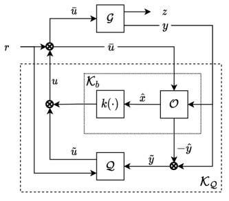
Figure 1: A version of the Youla-Kucera parameterization, where the Youla parameter $\mathcal{Q}$ augments an observer-based feedback controller $\mathcal{K}_{b}$.

III-B Assumptions

We make the following assumptions, drawing inspiration from [25, 28]:

1. Robustly stabilizing base controller: The closed-loop system composed of $\mathcal{G}$ in feedback with $\mathcal{K}_{b}$ is contracting and the map $r\mapsto z$ is Lipschitz.

2. Observer correctness: Given $\hat{x}_{0}=x_{0}$, the observer exactly replicates the plant dynamics. That is, $f(x_{t},\bar{u}_{t})=f_{o}(x_{t},\bar{u}_{t},c(x_{t}))\ \forall t\in\mathbb{N}$.

3. Contracting & Lipschitz observer: The observer $\mathcal{O}$ is contracting and the map $(\bar{u},y)\mapsto\hat{x}$ is Lipschitz.

4. Smooth maps: All functions are Lipschitz continuous and $f$ in (6) is continuously differentiable in $x$ on $\mathbb{R}^{n}$.

III-C Theoretical results

Our first main result is that augmenting a robustly stabilizing controller with a contracting and Lipschitz $\mathcal{Q}$ ensures the closed-loop system will also be contracting and Lipschitz. This allows optimization of the closed-loop response via $\mathcal{Q}$ while maintaining stability and robustness guarantees.

Theorem 1

Suppose that assumptions A1) to A4) hold and the Youla parameter $\mathcal{Q}$ is contracting and Lipschitz. Then the closed-loop system of $\mathcal{G}$ in (6) and $\mathcal{K}_{\mathcal{Q}}$ in (8) to (10) is contracting with transients and the map $r\mapsto z$ is Lipschitz.

The proof is provided in the appendix and can be summarized as follows. The observer error $\tilde{x}_{t}:=x_{t}-\hat{x}_{t}$ exponentially converges to zero since the plant trajectory $x$ is a particular solution of the observer, which is a contracting and Lipschitz system. This occurs regardless of $r_{t}$ and $\tilde{u}_{t}$. To prove contraction with transients, we show that the states of a contracting system exponentially converge given exponentially converging inputs, and apply this to $\mathcal{Q}$ and the closed-loop system under $\mathcal{K}_{b}$ (“base system”). We repeatedly apply Lipschitz properties of $\mathcal{Q}$ and the base system to prove that the closed-loop system under $\mathcal{K}_{\mathcal{Q}}$ is also Lipschitz.

One interesting question is whether the converse holds: that is, can a contracting and Lipschitz closed loop always be parameterized by a contracting and Lipschitz $\mathcal{Q}$? Our second main result shows that this is true under additional assumptions. We consider a perturbed nonlinear system

$$\mathcal{G}_{d}:\begin{cases}x_{t+1}=f(x_{t},u_{t}+r_{t})+d_{x_{t}}\\ y_{t}=c(x_{t})+d_{y_{t}}\end{cases}$$ (11)

where $d_{x_{t}}\in\mathbb{R}^{n}$ and $d_{y_{t}}\in\mathbb{R}^{p}$ are additive process and measurement disturbances, respectively. The following is a stronger version of assumption A1).

1. Robustness to disturbances: The closed-loop system $(r,d_{x},d_{y})\mapsto z$ composed of $\mathcal{G}_{d}$ in feedback with $\mathcal{K}_{b}$ is contracting and Lipschitz.

Theorem 2

Suppose that assumptions A2) to A5) hold. Then, any controller $\mathcal{K}$ forming a contracting and Lipschitz closed-loop map $(r,d_{x},d_{y})\mapsto z$ with $\mathcal{G}_{d}$ in (11) can be represented by (8) to (10) with contracting and Lipschitz $\mathcal{Q}$.

The proof follows by augmenting the robustly stabilizing controller $\mathcal{K}$ with an observer $\mathcal{O}$ to form a map $\mathcal{Q}_{\mathcal{K}}:(r,\tilde{y})\mapsto\tilde{u}$, which is contracting and Lipschitz by comparison with the closed-loop system under $\mathcal{K}$ (see appendix).

Remark 1

It is worth to noting that the closed-loop system is not guaranteed to be contracting and Lipschitz under bounded but unknown additive disturbances (see Example 1). This is because the observer error does not converge to zero in the presence of unknown disturbances, which is the key property required in Theorem 1. However, the closed-loop states will still be bounded under bounded additive disturbances [29, 30].

Example 1

Consider the following scalar system

$$\begin{split}\mathcal{G}:&\quad x_{t+1}=0.5\sin(x_{t})+\tilde{u}_{t}+d_{t}\\ \mathcal{K}_{\mathcal{Q}}:&\;\begin{cases}\hat{x}_{t+1}=0.5\sin(\hat{x}_{t})+\tilde{u}_{t}\\ \tilde{u}_{t}=10\tilde{y}=10(x-\hat{x}_{t})\end{cases}\end{split}$$

which is contracting for the case $d_{t}\equiv 0$. When $d_{t}\equiv 1$, the system converges to multiple solutions, hence the closed-loop system is not contracting under non-zero disturbances.

IV Numerical Experiments

We now examine the performance of the Youla-REN policy class on two RL problems: 1) magnetic suspension, and 2) inverting a rotary-arm pendulum. Each system is nonlinear and partially-observed, with different base controller designs to test the policy class under different architectures. We compare performance and robustness of three policy types:

1. Youla-REN: uses a contracting REN for the Youla parameter $\mathcal{Q}$ (see (9) and (10)).

2. Youla-$\gamma$REN: uses a REN with a Lipschitz upper bound of $\gamma$ (where $\gamma\to\infty$ recovers the contracting REN).

3. Feedback-LSTM: an LSTM network [31] augmenting the base controller via direct feedback of the measurement output, with $\tilde{u}=\mathcal{F}(y)$ for an LSTM system $\mathcal{F}$.

Since RENs are universal approximators of contracting and Lipschitz systems [12, Prop. 2], then by Theorem 1 the Youla-($\gamma$)REN parameterizes a set of contracting and Lipschitz closed-loops for partially-observed nonlinear systems. The Feedback-LSTM form is commonly used in deep RL (e.g: [3]) but provides no such stability or robustness guarantees. For more detail on contracting and Lipschitz parameterizations of RENs, see [13]. Our experiments were written in Julia using RobustEquilibriumNetworks.jl [32] and are available on github.

IV-A Problem setup

IV-A1 Learning objective

Let $z_{t}=p(x_{t})$ be a performance variable to be tracked for some function $p$. We formulated the RL tasks as minimizing a quadratic cost on the differences $\Delta z_{t}=z_{t}-z_{\mathrm{ref}}$, $\Delta u_{t}=u_{t}-u_{\mathrm{ref}}$ between performance variables and controls, and their desired reference values (respectively). That is,

$$\text{min.}\ E[J]\ \text{s.t.}\ J(x_{0})=\sum_{t=0}^{T-1}\left(|\Delta z_{t}|^{2}_{Q}+|\Delta u_{t}|^{2}_{R}\right)$$ (12)

where the cost function $J$ is weighted by matrices $Q$ and $R$. The expectation is over all possible initial conditions and random disturbances. We used $T=100$ time samples.

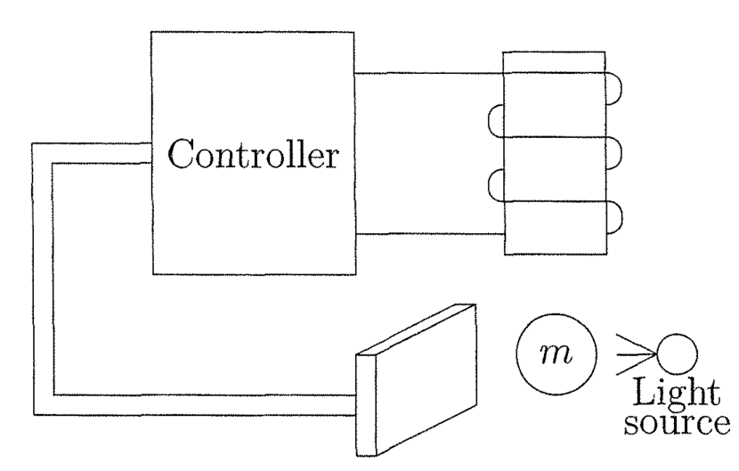
(a) 1D magnetic suspension.

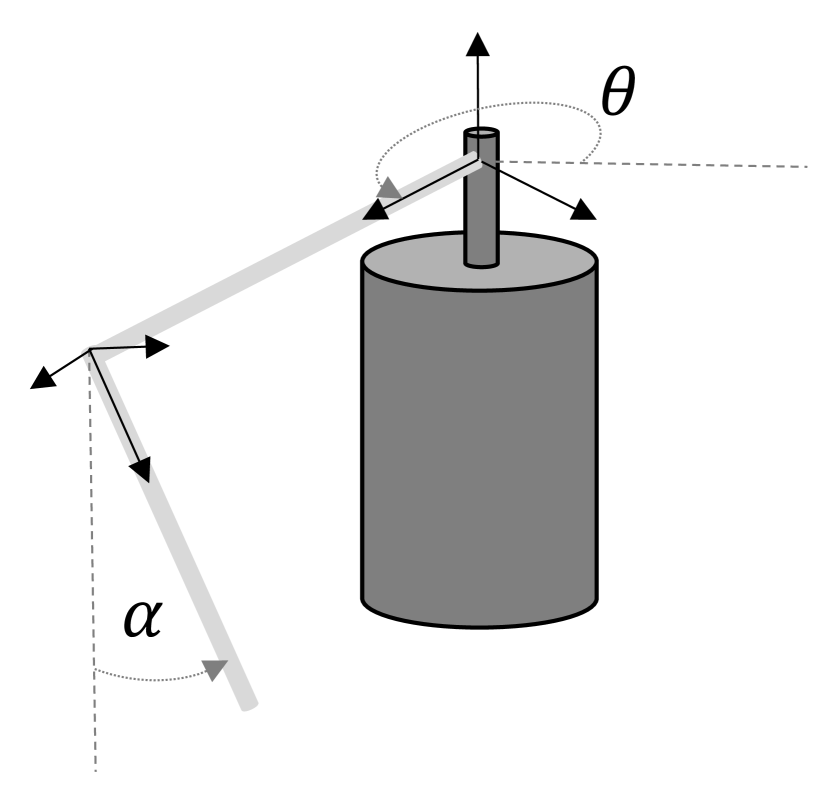
(b) Rotary-arm pendulum.

Figure 2: The two RL environments examined in Sec. IV: (a) a magnetic ball moving vertically under the influence of an electromagnet, and (b) a rotary-arm pendulum driven by a single motor on the rotating arm. The light source in (a) measures the ball position. Fig. 2(a) from [33].

IV-A2 Magnetic suspension

Consider the one-dimensional magnetic suspension system presented in [33], illustrated in Fig. 2(a). The system has three states (ball position, velocity, and coil current) and one input (coil voltage). Only the ball position and coil current are measured. We used the same nonlinear system model as in Exercise 13.27 of [33]. We added random noise to all states and measurements with standard deviations $5\times 10^{-4}$ and $10^{-3}$ (respectively).

The objective was to stabilize the ball at a height of 5 cm with minimal control effort. Our base controller consisted of a high-gain observer ([33, Sec. 14.5.2]) and a state-feedback controller designed with the backstepping and Lyapunov re-design methods outlined in [33, Sec. 14.2-14.3]. We encoded the learning objective in (12) with $z_{t}=x_{t}$, $Q=\mathrm{diag}(1/0.025^{2},0,0)$, $R=1/50^{2}$.

IV-A3 Rotary-arm pendulum

Next we considered the rotary-arm pendulum system in Fig. 2(b). The system has four states (rod angles and angular velocities) and one control input (motor voltage). Only the angles are measured. The system dynamics are presented in [34, Eqn. 31]. We added noise with standard deviation $10^{-2}$ to all states and measurements.

The control objective was to stabilize the pendulum in its (unstable) upright equilibrium, again with minimal control effort. We designed a state-feedback policy consisting of an energy-pumping controller to swing the pendulum arm upwards ([35, Eqn. 8]) and a static linear quadratic regulator to balance the pendulum within $30^{\circ}$ of the vertical. We completed the base controller with a high-gain observer. The learning objective was defined as per (12) with $z_{t}=(\cos\theta_{t},\sin\theta_{t},\cos\alpha_{t},\sin\alpha_{t})^{\top}$ for the arm and pendulum angles $\theta_{t},\alpha_{t}$ (respectively), and $Q=\mathrm{diag}(5,5,10,10)$, $R=0.01$. For small deviations from vertical, this is approximately a quadratic cost on $\Delta\theta_{t},\Delta\alpha_{t}$.

IV-B Results and discussion

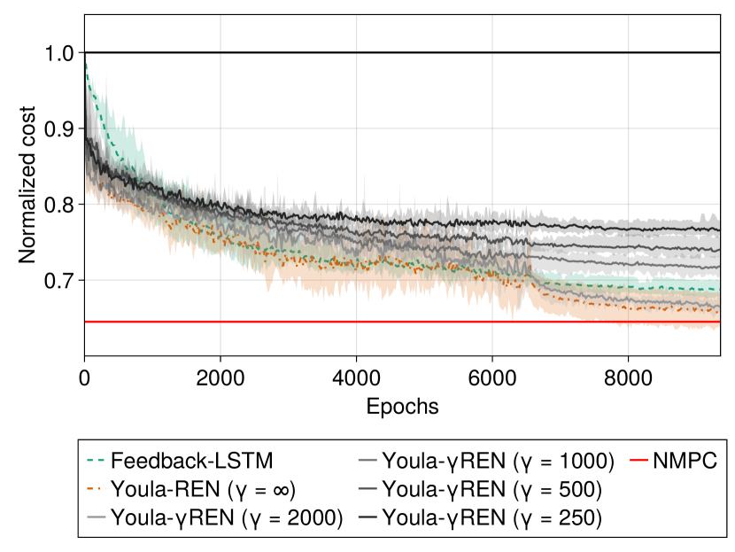
(a) Magnetic suspension.

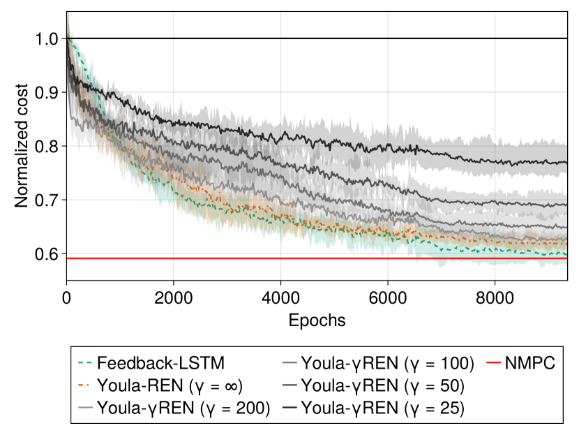
(b) Rotary-arm pendulum.

Figure 3: Loss curves showing the mean test cost vs. training epochs for policies trained on (a) the magnetic suspension problem and (b) the rotary-arm pendulum problem. Colored bands show the range over the six random seeds for each model, lines show the mean. Test cost is normalized by the base controller cost, indicated by the solid black line at 1.0.

IV-B1 Learning performance

Fig. 3 shows the mean test cost for each policy trained on the magnetic suspension and rotary-arm pendulum RL tasks. Policies were benchmarked against nonlinear model predictive controllers (NMPC), which are easy to design for low-dimensional problems. All of the learned policies show significant performance improvements over the base controller, and the best performing models reach the NMPC benchmarks. In particular, we see comparable performance between the Youla-REN and the Feedback-LSTM policy classes, with the Youla-REN achieving a lower cost on magnetic suspension, and the Feedback-LSTM performing slightly better on the rotary-arm pendulum. Together with the results of Sec. III, we therefore have a policy class that can perform as well as existing state-of-the-art methods on RL tasks for partially-observed nonlinear systems, while also providing stability guarantees for every policy trialled during training. Note that we have not compared the Youla-REN to an LSTM or REN in direct feedback without a base controller (the typical RL policy architecture) in Fig. 3. Training models in this configuration took significantly more epochs than the Youla and Feedback architectures, and achieved a worse final cost than even the base controllers on both tasks.

IV-B2 Robustness

One of the great advantages of the Youla-REN policy class is that we can control the performance-robustness trade-off by imposing a Lipschitz upper bound on the REN. The left panels in Figs. 4(a) and 4(b) show the effect of perturbing each trained policy with additive adversarial attacks of increasing size on the measurement signal $y_{t}$. The scatter plots to the right show the attack size required to meaningfully perturb each closed-loop system. We define a “critical” attack as one that shifts 1) the average ball position more than 1 cm from the target and 2) the average pendulum angle more than $30^{\circ}$ from the vertical in the magnetic suspension and rotary-arm pendulum tasks, respectively. Adversarial attacks were computed with minibatch gradient descent over a receding horizon of 10 time samples.

Comparing Figs. 3 and 4 demonstrates the effect of the Lipschitz bound on the performance-robustness trade-off. In Fig. 3, imposing a stronger Lipschitz bound (smaller $\gamma$) drives the Youla-$\gamma$REN policies to worse final costs. In Fig. 4, however, stronger Lipschitz bound can reliably lead to policies which are more robust to adversarial attacks, even if they perform worse in the unperturbed case. In particular, Fig. 4(b) shows that the base controller and Feedback-LSTM policies are highly sensitive to adversarial attacks in the rotary-arm pendulum environment. We suspect this is because the system has enough degrees of freedom to exhibit chaotic motion, and can be driven to extremely unstable closed-loop responses that are more difficult to recover from than in the magnetic suspension environment. Note that the relationship is not linear — imposing too strong a Lipschitz bound can lead to less robust policies (for example $\gamma=25$ in Fig. 4(b)). In practice, careful tuning of the imposed Lipschitz upper bound is required for a given problem.

IV-B3 Key results

These results emphasize the strength of the Youla-REN policy class in learning-based control tasks. We can take an existing stabilizing controller for a (nonlinear) dynamical system and learn a robust stabilizing feedback controller that improves some user-defined performance metric. Moreover, we can search over a space of contracting and Lipschitz closed-loops, guaranteeing stability at every step of the training process, and still achieve similar performance to existing methods which provide no such guarantees. Our approach is intuitive in that we can balance the performance-robustness trade-off by tuning the Lipschitz bound of the REN. It is versatile since we do not require special solution methods or projections during training. We therefore expect the Youla-REN to be well-suited to learning-based control in safety-critical robotic systems where performance and robustness are crucial to successful operation.

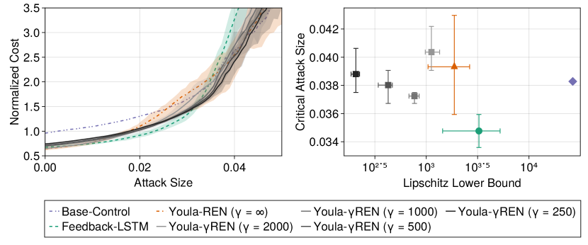
(a) Magnetic suspension.

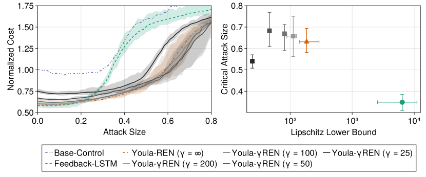
(b) Rotary-arm pendulum.

Figure 4: Normalized test cost vs. adversarial attack size for each of the trained models in Fig. 3. Lines show the average cost over the six random seeds for each model, with bands showing the range. Test cost is normalized by the cost of the (unperturbed) base controller. Scatter plots show the “critical” attack size required to perturb (a) the mean ball position 1 cm from its target and (b) the mean pendulum angle to $30^{\circ}$ from the vertical in each task, respectively. Error bars are for the six different random seeds for each model. The estimated Lipschitz lower bound of the base controller in (b) is extremely large and has been omitted from the scatter plot. Values of $\gamma$ in the legend are Lipschitz upper bounds.

Proofs of theorems

We first prove three auxiliary results. Each of these results are well-known and commonly referred to in the literature in various forms [29, 30, 36, 37]. We provide proofs of the particular discrete-time statements required in the proof of Theorem 1 for completeness.

Lemma 3

Consider a contracting system $\mathcal{T}$ given by (1). Then for any fixed input sequence $u\in\ell^{m}_{2e}$, any two state trajectories $x^{1},x^{2}\in\ell_{2e}^{n}$ exponentially converge to each other with a uniform rate and overshoot.

Proof:

Since $\mathcal{T}$ is contracting, it satisfies (2) and (3) with $c_{2}\geq c_{1}>0$ and $\alpha\in[0,1)$. Repeatedly applying (3) gives $V(x^{1}_{t},x^{2}_{t})\leq\alpha^{t}V(x^{1}_{0},x^{2}_{0})$ for all $t\in\mathbb{N}$ where $x^{1}_{0},x^{2}_{0}\in\mathbb{R}^{n}$ are the initial states of $x^{1},x^{2}$. Applying the upper and lower bounds in (2) then dividing through by $c_{1}$, we have

$$\absolutevalue{x^{1}_{t}-x^{2}_{t}}\leq\beta\alpha^{\frac{t}{2}}\absolutevalue{x^{1}_{0}-x^{2}_{0}}\ \forall t\in\mathbb{N}$$ (13)

where $\beta=\sqrt{c_{2}/c_{1}}$ is the overshoot. ∎

Lemma 4

Consider a contracting system $\mathcal{T}$ given by (1). Then for any $x_{0}\in\mathbb{R}^{n}$ and bounded inputs $u\in\ell_{2e}^{m}$, the states $x_{t}$ will also be bounded for all $t\in\mathbb{N}$.

Proof:

Re-write the dynamics of (1) as

$$x_{t+1}=\tilde{f}(x_{t})+d(x_{t},t)$$ (14)

where $\tilde{f}(x_{t}):=f(x_{t},0)$ and $d(x_{t},t):=f(x_{t},u_{t})-f(x_{t},0)$. We note two key facts about the system (14):

1. The system $x_{t+1}=\tilde{f}(x_{t})$ is an autonomous (time-invariant) contracting system and thus it will converge to a unique and bounded equilibrium $x^{\star}\in\mathbb{R}^{n}$ [29, Prop. (v), Sec. 3.7].

2. Since $u$ is bounded and $f$ is Lipschitz by assumption A4), then $d$ is also bounded and there exists $\bar{d}\in\mathbb{R}^{n}$ such that $\absolutevalue{d(x_{t},t)}\leq\bar{d}$ for all $t\in\mathbb{N}$.

Let $x^{1},x^{2}\in\ell_{2e}^{n}$ be solutions of the unperturbed dynamics $x_{t+1}=\tilde{f}(x_{t})$ and (14) (respectively) with initial states $x^{1}_{0},x^{2}_{0}\in\mathbb{R}^{n}$. We know that $x^{1}_{t}\rightarrow x^{*}$ uniformly and exponentially by Lemma 3. Therefore, it remains to prove that $\absolutevalue{x^{1}_{t}-x^{2}_{t}}$ is bounded for all $t\in\mathbb{N}$ if $u$ is bounded.

We apply the result of [30, Thm. 2.8] on (14) — that bounded additive perturbations to a contracting system generate bounded perturbations to its states — simplified here for an autonomous contracting system. Suppose there exists a uniformly positive-definite matrix $M(x_{t})=\Theta(x_{t})^{\top}\Theta(x_{t})\succ 0\ \forall\,x_{t}\in\mathbb{R}^{n}$, where $\Theta:\mathbb{R}^{n}\rightarrow\mathbb{R}^{n\times n}$ is a nonsingular matrix-valued function, that satisfies

$$a_{1}I\preceq M(x_{t})\preceq a_{2}I$$ (15)

$${\partialderivative{\tilde{f}}{x}}(x_{t})^{\top}M(x_{t+1}){\partialderivative{\tilde{f}}{x}}(x_{t})\preceq\sigma^{2}M(x_{t})$$ (16)

where $a_{2}\geq a_{1}>0$ and $\sigma\in[0,1)$. Then by [30, Thm. 2.8],

$$\absolutevalue{x^{1}_{t}-x^{2}_{t}}\leq C_{1}\sigma^{t}+\frac{\bar{d}}{1-\sigma}C_{2}$$ (17)

for some $C_{1},C_{2}\in\mathbb{R}^{+}$ where $C_{1}$ depends on the initial conditions $x^{1}_{0},x^{2}_{0}$.

A function $M(x_{t})$ satisfying (15) and (16) exists and is well-defined for the autonomous contracting system $x_{t+1}=\tilde{f}(x_{t})$, as explained below. Since the system is contracting, there exists a smooth function $V$ satisfying (2) and (3) with $c_{2}\geq c_{1}>0$ and $\alpha\in[0,1)$. We can re-write (3) as

$$V(x^{1}_{t+1},x^{2}_{t+1})-V(x^{1}_{t},x^{2}_{t})\leq-c_{3}\absolutevalue{x^{1}_{t}-x^{2}_{t}}^{2}$$

using the lower bound in (2), where $c_{3}=(1-\alpha)c_{1}$. Hence by [37, Thm. 11] and [38, Thm. 23.3] (both simplified for an autonomous system) there exists a nonsingular matrix-valued function $\Theta:\mathbb{R}^{n}\rightarrow\mathbb{R}^{n\times n}$ and constants $\mu,\eta,\rho\in\mathbb{R}^{+}$ such that

$$\eta I\preceq\Theta(x_{t})^{\top}\Theta(x_{t})\preceq\rho I$$ (18)

$$F(x_{t})^{\top}F(x_{t})-I\preceq-\mu I$$ (19)

for all $x_{t}\in\mathbb{R}^{n}$, where $\mu\in[0,1)$ and $F(x_{t})$ is given by

$$F(x_{t})=\Theta(x_{t+1}){\partialderivative{\tilde{f}}{x}}(x_{t})\Theta(x_{t})^{-1}.$$ (20)

Defining $M(x_{t})=\Theta(x_{t})^{\top}\Theta(x_{t})$, it is clear that (15) and (18) are identical if $a_{1}=\eta,a_{2}=\rho$, and (16) and (19) are equivalent if $\sigma^{2}=1-\mu$. Therefore, (17) holds and the states of a contracting system $\mathcal{T}$ given by (1) are bounded for bounded inputs $u\in\ell_{2e}^{m}$. ∎

Lemma 5

Consider a contracting system

$$\begin{cases}x_{t+1}=f(x_{t},u_{t},r_{t})\\ y_{t}=h(x_{t},u_{t},r_{t})\end{cases}$$ (21)

with state $x_{t}\in\mathbb{R}^{n}$, inputs $u_{t}\in\mathbb{R}^{m_{1}}$, $r_{t}\in\mathbb{R}^{m_{2}}$, and outputs $y\in\mathbb{R}^{p}$, where $f$ and $h$ are Lipschitz continuous. Further consider any fixed, bounded $r\in\ell_{2e}^{m_{2}}$ and any exponentially converging, bounded $u,v\in\ell_{2e}^{m_{1}}$ such that $\absolutevalue{u_{t}-v_{t}}\leq ba^{t}$ with $b\in\mathbb{R}^{+}$ and $a\in[0,1)$. Then the corresponding state and output trajectories $x,z\in\ell_{2e}^{n}$ and $y,p\in\ell_{2e}^{p}$ exponentially converge to each other (respectively) and satisfy

$$\absolutevalue{x_{t}-z_{t}} \leq\beta_{1}(x_{0},z_{0})\sigma_{1}^{t}$$ (22)

$$\absolutevalue{y_{t}-p_{t}} \leq\beta_{2}(x_{0},z_{0})\sigma_{2}^{t}$$ (23)

where $\beta_{i}:\mathbb{R}^{n}\times\mathbb{R}^{n}\rightarrow\mathbb{R}^{+}$ and $\sigma_{i}\in[0,1)$ for $i\in\{1,2\}$.

Proof:

Since the system is contracting, there exists a smooth function $V$ satisfying (2) and (3) with $c_{2}\geq c_{1}>0$ and $\alpha\in[0,1)$. First note that

$$V(x_{t+1},z_{t+1}) =V(f(x_{t},u_{t},r_{t}),f(z_{t},v_{t},r_{t}))$$

$$\leq V(f(x_{t},u_{t},r_{t}),f(z_{t},u_{t},r_{t}))+\absolutevalue{\Delta V}$$

where we introduced $\Delta V=V(f(x_{t},u_{t},r_{t}),f(z_{t},v_{t},r_{t}))-V(f(x_{t},u_{t},r_{t}),f(z_{t},u_{t},r_{t}))$. $V$ is locally Lipschitz (it is continuously differentiable) and all states of (21) are bounded as per Lemma 4. Hence, there exists some finite upper bound $\gamma_{V}\in\mathbb{R}^{+}$ for a given $z,u,v,r$ such that

$$\absolutevalue{\Delta V}\leq\gamma_{V}\absolutevalue{f(z_{t},v_{t},r_{t})-f(z_{t},u_{t},r_{t})}\quad\forall\,t\in\mathbb{N}.$$

Since $f$ is globally Lipschitz then $\absolutevalue{\Delta V}\leq\gamma_{V}\gamma_{f}\absolutevalue{v_{t}-u_{t}}$ for some $\gamma_{f}\in\mathbb{R}^{+}$ and so $\absolutevalue{\Delta V}\leq\bar{b}a^{t}$ where $\bar{b}=b\gamma_{V}\gamma_{f}$. Applying (3), we therefore have

$$V(x_{t+1},z_{t+1})\leq\alpha V(x_{t},z_{t})+\bar{b}a^{t}.$$ (24)

It is clear from (24) that $V$ is upper-bounded by the particular solution of a two-state linear system

$$q_{t+1}=\matrixquantity[\alpha&\bar{b}\\ 0&a]q_{t}\quad\text{with}\quad q_{0}=\matrixquantity[V(x_{0},z_{0})\\ 1].$$

This system is stable since $\alpha,a\in[0,1)$, and hence $V$ will be exponentially upper-bounded for all $t$. In fact, we can compute the analytic solution of this system. Using the fact that $\sum_{k=0}^{t-1}\alpha^{t-k}a^{k}=(\alpha^{t}-a^{t})/(\alpha-a)$, we have

$$V(x_{t},z_{t})\leq\alpha^{t}V(x_{0},z_{0})+\bar{b}\cdot\frac{\alpha^{t}-a^{t}}{\alpha-a}.$$ (25)

Applying the upper and lower-bounds on $V$ and dividing through by $c_{1}$ shows that

$$\absolutevalue{x_{t}-z_{t}}^{2}\leq\frac{c_{2}}{c_{1}}\alpha^{t}\absolutevalue{x_{0}-z_{0}}^{2}+\frac{\bar{b}}{c_{1}}\cdot\frac{\alpha^{t}-a^{t}}{\alpha-a}.$$ (26)

Taking the square root gives an inequality in the form of (22), where $\beta_{1}:\mathbb{R}^{n}\times\mathbb{R}^{n}\rightarrow\mathbb{R}^{+}$ and $\sigma_{1}\in[0,1)$ take different values depending on $\alpha$ and $a$:

1. If $\alpha\neq a$, then (22) is satisfied with $\sigma_{1}=\sqrt{\max(\alpha,a)}$ and $\beta_{1}^{2}=\frac{c_{2}}{c_{1}}\absolutevalue{x_{0}-z_{0}}^{2}+\frac{\bar{b}}{c_{1}\absolutevalue{\alpha-a}}.$

2. If $\alpha=a$, the sum of terms giving (25) collapses to $\sum_{k=0}^{t-1}\alpha^{t}=t\alpha^{t}$ and (26) becomes

   $$\absolutevalue{x_{t}-z_{t}}^{2}\leq\left(\frac{c_{2}}{c_{1}}\absolutevalue{x_{0}-z_{0}}^{2}+\frac{\bar{b}}{c_{1}}t\right)\alpha^{t}.$$

   The function on the right-hand side can be uniformly and exponentially upper-bounded by $\beta_{1}\sigma_{1}^{t}$ where $\sigma_{1}\in[\alpha,1)$, $\beta_{1}\in\mathbb{R}^{+}$ since the exponential function $(\sigma_{1}/\alpha)^{t}$ dominates the linear term for sufficiently large $t$. Hence there exists a $T\in\mathbb{R}^{+}$ such that (22) is satisfied with $\beta_{1}^{2}=\frac{c_{2}}{c_{1}}\absolutevalue{x_{0}-z_{0}}^{2}+\frac{\bar{b}}{c_{1}}T$ and $\sigma_{1}\in[\alpha,1)$.

The result (23) follows from (22) and $\absolutevalue{u_{t}-v_{t}}\leq ba^{t}$ by noting that the output function $h$ in (21) is Lipschitz. ∎

Proof:

(Theorem 1) Let $\bar{x}_{t}=(x_{t}^{\top},\tilde{x}_{t}^{\top},q_{t}^{\top})^{\top}$ be the state of the closed-loop system under $\mathcal{K}_{\mathcal{Q}}$, where $\tilde{x}_{t}=x_{t}-\hat{x}_{t}$ is the observer error. The closed-loop system maps $r\mapsto z$ with

$$\mathcal{G}_{\mathrm{CL}}:\begin{cases}x_{t+1}=f(x_{t},\bar{u}_{t})\\ \tilde{x}_{t+1}=f(x_{t},\bar{u}_{t})-f_{o}(x_{t}-\tilde{x}_{t},\bar{u}_{t},c(x_{t}))\\ q_{t+1}=f_{q}(q_{t},r_{t},c(x_{t})-c(x_{t}-\tilde{x}_{t}))\\ z_{t}=(x_{t}^{\top},(k(x_{t}-\tilde{x}_{t})+\tilde{u}_{t})^{\top})^{\top}\end{cases}$$ (27)

where $\bar{u}_{t}=k(x_{t}-\tilde{x}_{t})+\tilde{u}_{t}+r_{t}$ and $\tilde{u}_{t}=h_{q}(q_{t},r_{t},c(x_{t})-c(x_{t}-\tilde{x}_{t}))$. We will show that $\mathcal{G}_{\mathrm{CL}}$ is contracting and Lipschitz with transients due to initial conditions as per Definitions 2 and 3, respectively.

Proof of contraction

Consider the observer error $\tilde{x}$ for a single trajectory. Since the observer satisfies the correctness assumption A2), we can write $\tilde{x}=\mathcal{O}_{x_{0}}(\bar{u},y)-\mathcal{O}_{\hat{x}_{0}}(\bar{u},y)$, where the subscripts on $\mathcal{O}$ distinguish between the initial system and observer states. The inputs $\bar{u}=u+r$ and $y$ are the same for both the true and estimated state trajectories $x$ and $\hat{x}$ (respectively). Therefore by Lemma 3, there exists a $\beta\in\mathbb{R}^{+}$ and $\alpha\in[0,1)$ such that $\absolutevalue{\tilde{x}_{t}}\leq\beta\alpha^{t}\absolutevalue{\tilde{x}_{0}}$ since the observer is contracting by A3).

Now consider any two state trajectories $\bar{x}^{1},\bar{x}^{2}\in\ell_{2e}$ of the closed-loop system $\mathcal{G}_{\mathrm{CL}}$ starting from initial states $\bar{x}^{1}_{0},\bar{x}^{2}_{0}\in\mathbb{R}^{2n+q}$ and given the same input sequence $r\in\ell^{m}_{2e}$. The observer errors exponentially converge to one another since

$$\absolutevalue{\tilde{x}^{1}_{t}-\tilde{x}^{2}_{t}}\leq\beta\alpha^{t}(\absolutevalue{\tilde{x}^{1}_{0}}+\absolutevalue{\tilde{x}^{2}_{0}})=:\bar{\beta}(\tilde{x}^{1}_{0},\tilde{x}^{2}_{0})\alpha^{t}.$$

The same is true for the innovations signals

$$\absolutevalue{\tilde{y}^{1}_{t}-\tilde{y}^{2}_{t}}\leq\gamma_{c}\bar{\beta}(\tilde{x}^{1}_{0},\tilde{x}^{2}_{0})\alpha^{t},$$ (28)

where $\gamma_{c}$ is the Lipschitz bound of the measurement function $c(\cdot)$ from (6).

We now repeatedly apply Lemma 5 to prove the result. Since $\tilde{u}=\mathcal{Q}(r,\tilde{y})$ is contracting, $\absolutevalue{\tilde{y}^{1}_{t}-\tilde{y}^{2}_{t}}$ exponentially converges to zero, and $r^{1}=r^{2}$ is bounded, then by Lemma 5

$$\absolutevalue{\tilde{u}^{1}_{t}-\tilde{u}^{2}_{t}}\leq\beta_{q}(q^{1}_{0},q^{2}_{0},\tilde{x}^{1}_{0},\tilde{x}^{2}_{0})\alpha_{q}^{t}$$

with $\beta_{q}\geq 0$ and $\alpha\in[0,1)$. By assumption A1), the closed-loop system under the base controller mapping $\tilde{u},r\mapsto z$ is also contracting. Therefore, the states $(x_{t}^{i\top},\tilde{x}_{t}^{i\top})^{\top}$ with $i\in\{1,2\}$ also exponentially converge to one another with uniform rate and an overshoot dependent on initial conditions, again by Lemma 5. Hence there exists a $\beta_{\mathrm{CL}}(\bar{x}^{1}_{0},\bar{x}^{2}_{0})\geq 0$ and $\alpha_{\mathrm{CL}}\in[0,1)$ such that

$$\absolutevalue{\bar{x}^{1}_{0}-\bar{x}^{2}_{0}}\leq\beta_{\mathrm{CL}}(\bar{x}^{1}_{0},\bar{x}^{2}_{0})\alpha_{\mathrm{CL}}^{t},$$ (29)

so $\mathcal{G}_{\mathrm{CL}}$ is contracting with transients.

Proof of Lipschitz

Consider two trajectories $z^{1},z^{2}\in\ell_{2e}$ of the closed-loop system starting from initial states $\bar{x}^{1}_{0},\bar{x}^{2}_{0}\in\mathbb{R}^{2n+q}$ with inputs $r_{1},r_{2}\in\ell^{m}_{2e}$, respectively. Denote $\Delta z=z^{1}-z^{2}$ and similarly for all other variables. By assumption A1), the closed-loop system under the base controller is Lipschitz with respect to any inputs $(r+\tilde{u})\in\ell_{2e}^{m}$, hence $\exists\ \gamma\in\mathbb{R}^{+}$ and $\kappa_{1}(s^{1}_{0},s^{2}_{0})\geq 0$ such that

$$\norm{\Delta z}_{T} \leq\gamma\norm{(r^{1}+\tilde{u}^{1})-(r^{2}+\tilde{u}^{2})}_{T}+\kappa_{1}(s^{1}_{0},s^{2}_{0})$$

$$\leq\gamma\norm{\Delta r}_{T}+\gamma\norm{\Delta\tilde{u}}_{T}+\kappa_{1}(s^{1}_{0},s^{2}_{0}).$$

Since $\mathcal{Q}$ is Lipschitz by assumption, then similarly $\exists\ \gamma_{q_{r}},\gamma_{q_{y}}\in\mathbb{R}^{+}$ and $\kappa_{2}(q^{1}_{0},q^{2}_{0})\geq 0$ such that

$$\norm{\tilde{u}}_{T}\leq\gamma_{q_{r}}\norm{\Delta r}_{T}+\gamma_{q_{y}}\norm{\Delta\tilde{y}}_{T}+\kappa_{2}(q^{1}_{0},q^{2}_{0})$$

Note further that $\tilde{y}=c(x)-c(\hat{x})$ (where $c(\cdot)$ acts element-wise on signals) so $\norm{\Delta\tilde{y}}_{T}\leq\gamma_{c}\norm{\Delta\tilde{x}}_{T}$ since $c(\cdot)$ is Lipschitz with bound $\gamma_{c}\in\mathbb{R}^{+}$ by assumption A4). Combining these expressions, we have that

$$\norm{\Delta z}_{T}\leq\gamma(1+\gamma_{q_{r}})\norm{\Delta r}_{T}+\tilde{\gamma}\norm{\Delta\tilde{x}}_{T}+\kappa_{3}(\bar{x}^{1}_{0},\bar{x}^{2}_{0})$$ (30)

where $\tilde{\gamma}=\gamma\gamma_{q_{y}}\gamma_{c}$ and $\kappa_{3}=\kappa_{1}+\gamma\kappa_{2}$. Since the observer error satisfies $\absolutevalue{\tilde{x}_{t}}\leq\beta\alpha^{t}\absolutevalue{\tilde{x}_{0}}$ for any $\tilde{u},r$, then there exists a finite $\Gamma(\tilde{x}_{0})\geq 0$ such that $\norm{\tilde{x}}_{T}\leq\Gamma(\tilde{x}_{0})$. Hence $\norm{\Delta\tilde{x}}_{T}\leq\Gamma(\tilde{x}^{1}_{0})+\Gamma(\tilde{x}^{2}_{0})$ and substituting into (30) gives

$$\norm{\Delta z}_{T}\leq\bar{\gamma}\norm{\Delta r}_{T}+\kappa_{4}(\bar{x}^{1}_{0},\bar{x}^{2}_{0})$$ (31)

where $\bar{\gamma}=\gamma(1+\gamma_{q_{r}})$ and $\kappa_{4}=\tilde{\gamma}(\Gamma(x^{1}_{0},\hat{x}^{1}_{0})+\Gamma(x^{2}_{0},\hat{x}^{2}_{0}))+\kappa_{3}$. The closed-loop system $\mathcal{G}_{\mathrm{CL}}$ is therefore Lipschitz with the effect of initial conditions captured by $\kappa_{4}\geq 0$. ∎

Proof:

(Theorem 2) Consider the closed-loop system of the disturbed plant $\mathcal{G}_{d}$ from (11) in feedback with a robustly stabilizing feedback controller

$$\mathcal{K}:\begin{cases}\phi_{t+1}=h(\phi_{t},y_{t})\\ u_{t}=g(\phi_{t},y_{t})\end{cases}$$ (32)

with states $\phi_{t}\in\mathbb{R}^{k}$. The closed-loop system $\bar{\mathcal{G}}_{\mathrm{CL}}:(r,d_{x},d_{y})\mapsto z$ is given by

$$\bar{\mathcal{G}}_{\mathrm{CL}}:\begin{cases}x_{t+1}=f(x_{t},g(\phi_{t},c(x_{t})+d_{y_{t}})+r_{t})+d_{x_{t}}\\ \phi_{t+1}=h(\phi_{t},c(x_{t})+d_{y_{t}})\\ z_{t}=(x_{t}^{\top},g(\phi_{t},c(x_{t})+d_{y_{t}})^{\top})^{\top}.\end{cases}$$ (33)

The system $\bar{\mathcal{G}}_{\mathrm{CL}}$ is contracting and Lipschitz by assumption. We now aim to show that $\mathcal{K}$ can be represented by a Youla controller (9) – (10) parameterized by a contracting and Lipschitz $\mathcal{Q}_{\mathcal{K}}$. By augmenting $\mathcal{K}$ with a Lipschitz state-feedback controller $k(\cdot)$ and an observer satisfying assumptions A2) to A4), we can construct a map $\mathcal{Q}_{\mathcal{K}}:(r,\tilde{y})\mapsto\tilde{u}$ using the fact that $y_{t}=\tilde{y}_{t}+c(\hat{x}_{t})$ and $\tilde{u}_{t}=\bar{u}_{t}-k(\hat{x}_{t})$. This gives

$$\mathcal{Q}_{\mathcal{K}}:\begin{cases}\hat{x}_{t+1}=f_{o}(\hat{x}_{t},g(\phi_{t},c(\hat{x}_{t})+\tilde{y}_{t})+r_{t},c(\hat{x}_{t}))+\Delta f_{o}\\ \phi_{t+1}=h(\phi_{t},c(\hat{x}_{t})+\tilde{y}_{t})\\ \tilde{u}_{t}=g(\phi_{t},c(\hat{x}_{t})+\tilde{y}_{t})-k(\hat{x}_{t}).\end{cases}$$ (34)

where $\Delta f_{o}:=f_{o}(\hat{x}_{t},u_{t}+r_{t},c(\hat{x}_{t})+\tilde{y})-f_{o}(\hat{x}_{t},u_{t}+r_{t},c(\hat{x}_{t}))$. Note that $\mathcal{Q}_{\mathcal{K}}$ does not change the control signal $u_{t}$ since $\tilde{u}_{t}+k(\hat{x}_{t})=g(\phi_{t},y_{t})$ by construction. We show that $\mathcal{Q}_{\mathcal{K}}$ is contracting and Lipschitz by comparing it to $\bar{\mathcal{G}}_{\mathrm{CL}}$. Make the substitution $\hat{x}_{t}\leftrightarrow x_{t}$, $\tilde{y}_{t}\leftrightarrow d_{y_{t}}$, $\Delta f_{o}\leftrightarrow d_{x_{t}}$. Then the state dynamics of $\mathcal{Q}_{\mathcal{K}}$ and $\bar{\mathcal{G}}_{\mathrm{CL}}$ are identical after applying assumption A2), and hence $\mathcal{Q}_{\mathcal{K}}$ is contracting.

It remains to show that $\mathcal{Q}_{\mathcal{K}}:(r,\tilde{y})\rightarrow\tilde{u}$ is Lipschitz. We know $(r,d_{x},d_{y})\mapsto z$ is Lipschitz, and hence so too is $(r,\tilde{y})\mapsto z$ following our transformation, noting that the norm of $\Delta f_{o}$ is linearly bounded by $\tilde{y}$ since $f_{o}$ is Lipschitz. Considering $z\mapsto\tilde{u}$, note that under $x\leftrightarrow\hat{x}$ then $z=(\hat{x}^{\top},u^{\top})^{\top}$ and $u=\tilde{u}+k(\hat{x})$ so $\tilde{u}=k([I,0]z)-[0,I]z$ where $k(\cdot)$ acts element-wise on signals. Since $k(\cdot)$ is a Lipschitz function, then the map $z\mapsto\tilde{u}$ is Lipschitz and hence so too is $\mathcal{Q}_{\mathcal{K}}:(r,\tilde{y})\mapsto\tilde{u}$. ∎

Model configurations and training details

We compared the three model architectures on each RL task outlined in Section IV. We selected four Lipschitz bounds for the Youla-$\gamma$RENs on each task to compare the effect of imposing robustness constraints. Similar numbers of model parameters were used for a fair comparison. LSTM models were allocated 28 cell units, while the RENs and $\gamma$RENs were given 32 states and 64 neurons. We found that reducing the dimensionality of one of the REN parameters (the $X$ matrix in [13, Eqn. 23]) from ($128\times 128$) to ($16\times 128$) accelerated learning and improved performance in the Youla-REN and Youla-$\gamma$RENs. ReLU activation functions were used for all RENs models.

We chose to use a separate, de-tuned observer to compute the innovations in the magnetic suspension task instead of the base observer. This slowed the contraction rate of the innovations sequence, giving the network more samples with a non-zero input signal to affect the controls. This does not violate any assumptions outlined in Sec. III, since our only requirements for the observer were only that it satisfied the correctness, contraction, and Lipschitz properties A2) to A4).

We trained our models using a version of the Augmented Random Search (ARS)-v1 algorithm from [39]. Each model was trained with six random seeds to account for variability in the initialization. We averaged gradient estimates over 16 perturbation directions at each training epoch, using batches of 50 random initial conditions to approximate the expected costs, and clipped gradients to an $\ell^{2}$ norm of 10. A batch size of 100 was used for the test cost. Models were trained with the ADAM optimizer [40]. Learning rates and ARS exploration magnitudes were tuned by sweeping over a wide range from $10^{-5}$ to $10^{-1}$. The best-performing combinations for each model and task are provided in Table I. Learning rates were decreased by a factor of 10 after 70% of the total epochs to verify that the models had converged.

	Magnetic Suspension			Rotary Pendulum
Model	$\gamma$	$\alpha$	$\sigma$	$\gamma$	$\alpha$	$\sigma$
Feedback-LSTM	-	0.01	0.01	-	0.01	0.02
Youla-REN	$\infty$	0.005	0.01	$\infty$	0.01	0.05
Youla-$\gamma$REN	2000	0.005	0.01	200	0.01	0.05
	1000	0.005	0.05	100	0.01	0.05
	500	0.005	0.05	50	0.01	0.05
	250	0.005	0.05	25	0.01	0.05

TABLE I: Learning rates $\alpha$, ARS exploration magnitudes $\sigma$, and imposed Lipschitz upper bounds $\gamma$ on the two RL tasks.

References

- [1] V. Mnih, K. Kavukcuoglu, D. Silver, A. A. Rusu, J. Veness, M. G. Bellemare, A. Graves, M. Riedmiller, A. K. Fidjeland, G. Ostrovski, S. Petersen, C. Beattie, A. Sadik, I. Antonoglou, H. King, D. Kumaran, D. Wierstra, S. Legg, and D. Hassabis, “Human-level control through deep reinforcement learning,” Nature, vol. 518, pp. 529–533, 2 2015.
- [2] D. Silver, J. Schrittwieser, K. Simonyan, I. Antonoglou, A. Huang, A. Guez, T. Hubert, L. Baker, M. Lai, A. Bolton, Y. Chen, T. Lillicrap, F. Hui, L. Sifre, G. V. D. Driessche, T. Graepel, and D. Hassabis, “Mastering the game of go without human knowledge,” Nature, vol. 550, pp. 354–359, 10 2017.
- [3] J. Siekmann, Y. Godse, A. Fern, and J. Hurst, “Sim-to-real learning of all common bipedal gaits via periodic reward composition,” 11 2021.
- [4] B. Hu, K. Zhang, N. Li, M. Mesbahi, M. Fazel, and T. Başar, “Toward a theoretical foundation of policy optimization for learning control policies,” https://doi.org/10.1146/annurev-control-042920-020021, vol. 6, pp. 123–158, 5 2023.
- [5] B. D. Anderson, “From youla-kucera to identification, adaptive and nonlinear control,” Automatica, vol. 34, pp. 1485–1506, 12 1998.
- [6] J. W. Roberts, I. R. Manchester, and R. Tedrake, “Feedback controller parameterizations for reinforcement learning,” pp. 310–317, 2011.
- [7] J. I. Imura and T. Yoshikawa, “Parametrization of all stabilizing controllers of nonlinear systems,” Systems & Control Letters, vol. 29, pp. 207–213, 1 1997.
- [8] L. Furieri, C. L. Galimberti, and G. Ferrari-Trecate, “Neural system level synthesis: Learning over all stabilizing policies for nonlinear systems,” pp. 2765–2770, 1 2023.
- [9] J. B. Moore and L. Irlicht, “Coprime factorization over a class of nonlinear systems,” Proceedings of the American Control Conference, vol. 4, pp. 3071–3075, 1992.
- [10] F. Blanchini, D. Casagrande, and S. Miani, “Parametrization of all stabilizing compensators for absorbable nonlinear systems,” Proceedings of the IEEE Conference on Decision and Control, pp. 5943–5948, 2010.
- [11] R. Wang and I. R. Manchester, “Youla-ren: Learning nonlinear feedback policies with robust stability guarantees,” Proceedings of the American Control Conference, vol. 2022-June, pp. 2116–2123, 2022.
- [12] R. Wang, N. H. Barbara, M. Revay, and I. R. Manchester, “Learning over all stabilizing nonlinear controllers for a partially-observed linear system,” IEEE Control Systems Letters, pp. 1–1, 2022.
- [13] M. Revay, R. Wang, and I. R. Manchester, “Recurrent equilibrium networks: Flexible dynamic models with guaranteed stability and robustness,” IEEE Transactions on Automatic Control, pp. 1–16, 2023.
- [14] D. C. Youla, J. J. Bongiorno, and H. A. Jabr, “Modern wiener-hopf design of optimal controllers — part ii: The multivariable case,” IEEE Transactions on Automatic Control, vol. 21, pp. 319–338, 1976.
- [15] F. Li, S. Yuan, F. Qian, Z. Wu, H. Pu, M. Wang, J. Ding, and Y. Sun, “Adaptive deterministic vibration control of a piezo-actuated active–passive isolation structure,” Applied Sciences 2021, Vol. 11, Page 3338, vol. 11, p. 3338, 4 2021.
- [16] I. Mahtout, F. Navas, V. Milanes, and F. Nashashibi, “Advances in youla-kucera parametrization: A review,” Annual Reviews in Control, vol. 49, pp. 81–94, 1 2020.
- [17] J. Miller and M. Hardt, “Stable recurrent models,” 7th International Conference on Learning Representations, ICLR 2019, 5 2018.
- [18] P. Pauli, A. Koch, J. Berberich, P. Kohler, and F. Allgower, “Training robust neural networks using lipschitz bounds,” IEEE Control Systems Letters, vol. 6, pp. 121–126, 2022.
- [19] J. N. Knight and C. Anderson, “Stable reinforcement learning with recurrent neural networks,” Journal of Control Theory and Applications, vol. 9, pp. 410–420, 8 2011.
- [20] N. Junnarkar, H. Yin, F. Gu, M. Arcak, and P. Seiler, “Synthesis of stabilizing recurrent equilibrium network controllers,” pp. 7449–7454, 1 2023.
- [21] A. D. Paice and J. B. Moore, “On the youla-kucera parametrization for nonlinear systems,” Systems & Control Letters, vol. 14, pp. 121–129, 2 1990.
- [22] G. Chen and R. J. de Figueiredo, “Construction of the left coprime fractional representation for a class of nonlinear control systems,” Systems & Control Letters, vol. 14, pp. 353–361, 4 1990.
- [23] A. D. Paice and A. J. van der Schaft, “Stable kernel representations as nonlinear left coprime factorizations,” Proceedings of the IEEE Conference on Decision and Control, vol. 3, pp. 2786–2791, 1994.
- [24] A. D. Paice and A. J. V. D. Schaft, “The class of stabilizing nonlinear plant controller pairs,” IEEE Transactions on Automatic Control, vol. 41, pp. 634–645, 1996.
- [25] K. Fujimoto and T. Sugie, “Characterization of all nonlinear stabilizing controllers via observer-based kernel representations,” Automatica, vol. 36, pp. 1123–1135, 8 2000.
- [26] K. Fujimoto and T. Sugie, “State-space characterization of youla parametrization for nonlinear systems based on input-to-state stability,” Proceedings of the IEEE Conference on Decision and Control, vol. 3, pp. 2479–2484, 1998.
- [27] M. Revay, R. Wang, and I. R. Manchester, “A convex parameterization of robust recurrent neural networks,” IEEE Control Systems Letters, vol. 5, pp. 1363–1368, 10 2021.
- [28] B. Yi, R. Wang, and I. R. Manchester, “Reduced-order nonlinear observers via contraction analysis and convex optimization,” IEEE Transactions on Automatic Control, vol. 67, pp. 4045–4060, 8 2022.
- [29] W. Lohmiller and J. J. E. Slotine, “On contraction analysis for non-linear systems,” Automatica, vol. 34, pp. 683–696, 6 1998.
- [30] H. Tsukamoto, S. J. Chung, and J. J. E. Slotine, “Contraction theory for nonlinear stability analysis and learning-based control: A tutorial overview,” Annual Reviews in Control, vol. 52, pp. 135–169, 1 2021.
- [31] S. Hochreiter and J. Schmidhuber, “Long short-term memory,” Neural Computation, vol. 9, pp. 1735–1780, 11 1997.
- [32] N. H. Barbara, M. Revay, R. Wang, J. Cheng, and I. R. Manchester, “Robustneuralnetworks.jl: a package for machine learning and data-driven control with certified robustness,” arXiv preprint arXiv:2306.12612, 6 2023.
- [33] H. K. Khalil, Nonlinear systems; 3rd ed. Prentice-Hall, 2002. The book can be consulted by contacting: PH-AID: Wallet, Lionel.
- [34] B. S. Cazzolato and Z. Prime, “On the dynamics of the furuta pendulum,” Journal of Control Science and Engineering, vol. 2011, 2011.
- [35] K. J. Åström and K. Furuta, “Swinging up a pendulum by energy control,” Automatica, vol. 36, pp. 287–295, 2 2000.
- [36] F. Bullo, Contraction Theory for Dynamical Systems. Kindle Direct Publishing, 1.0 ed., 2022.
- [37] D. N. Tran, B. S. Rüffer, and C. M. Kellett, “Convergence properties for discrete-time nonlinear systems,” IEEE Transactions on Automatic Control, vol. 64, pp. 3415–3422, 8 2019.
- [38] W. J. Rugh, Linear system theory / Wilson J. Rugh. Prentice Hall,, 2nd ed. ed., 1996. Includes bibliographical references and indexes.;Chapter Dependence Chart – 1. Mathematical Notation and Review – 2. State Equation Representation – 3. State Equation Solution – 4. Transition Matrix Properties – 5. Two Important Cases – 6. Intern.
- [39] H. Mania, A. Guy, and B. Recht, “Simple random search of static linear policies is competitive for reinforcement learning,” Advances in Neural Information Processing Systems, vol. 31, 2018.
- [40] D. P. Kingma and J. L. Ba, “Adam: A method for stochastic optimization,” International Conference on Learning Representations, ICLR, 12 2015.