Finite temperature second harmonic generation in Kitaev magnets

Abstract

We study electric field induced second harmonic generation (2HG) in the Kitaev model. This frustrated magnet hosts a quantum spin-liquid, featuring fractionalization in terms of mobile Majorana fermion and static $\mathbb{Z}_{2}$ flux-vison elementary excitations. We show that finite temperature 2HG allows to probe characteristic features of both fractional quasiparticle types. In the homogeneous flux state at low-temperatures, the 2HG susceptibility displays an oscillatory spectrum, which is set by only the fermionic excitations and is subject to temperature induced Fermi-blocking, generic to all higher harmonic generation (HHG). In the intermediate to high temperature range, intrinsic randomness, which emerges from thermally excited visons leads to drastic changes of the 2HG susceptibility, resulting from resonance decoupling over a wide range of energies. At the flux proliferation crossover, we suggest an interpolation between these two temperature regimes. Our results satisfy previously established symmetries for electric field induced 2HG in Kitaev magnets.

I Introduction

Nonlinear optical (NLO) spectroscopy is a diverse tool of many interests. In particular, second harmonic generation (2HG) has traditionally served as a probe to study inversion symmetry breaking [1]. Lately, this has played an eminent role in bulk graphene materials [2, 3, 4, 5], layered transition metal dichalcogenides [6, 7, 8, 9, 10], and transition metal monopnictide Weyl semimetals [11]. Probing inversion symmetry breaking by 2HG can even be related to local properties [12]. Apart from 2HG, photovoltaic shift currents, e.g., in ferroelectrics [13, 14] and topological insulators [15] are another second order NLO response of interest which is of similar sensitivity to symmetries. Photogalvanic currents have been considered not only in the charge, but also in the spin channel, e.g., for bilayer trihalides [16].

Beyond exploring symmetries with low-order HG, the complete time-dependence of the NLO response is of interest due to its relations to Floquet group theory and Floquet topological insulators [17, 18, 19]. This is because the allowed emissions from higher harmonic generation (HHG) can be analyzed in terms of certain spatiotemporal, dynamical symmetries of time-periodically driven systems [17, 20, 21]

Lately, two-dimensional coherent NLO spectroscopy (2DCS), which is a third-order echo response [22, 23], has come into focus, for accessing quasiparticle spectra and interactions. This pertains not only to semiconductors [23], molecules [24], and disordered many-body systems [25]. Instead, direct coupling of the driving external magnetic fields to the spin of correlated magnets has allowed to consider magnons [26], kinks [27], spinons [28], fractons [29], Majorana fermions and visons [30] by 2DCS and also by a related second-order spectroscopy [31]. Such applications have linked NLO spectroscopy to the very timely topics of quantum spin-liquids (QSL) and fractionalization [32].

In the context of QSLs, the Kitaev magnet [33] is of particular interest [35, 34]. This frustrated magnet hosts a QSL due to an exact fractionalization of spin in terms of two types of elementary excitations, namely mobile Majorana matter and $\mathbb{Z}_{2}$ gauge flux which is localized in the absence of external magnetic fields [33]. It is realized by an Ising model on the honeycomb lattice with bond-directional anisotropy and may serve as a low-energy spin model for certain Mott-Hubbard insulators with strong spin-orbit coupling [36]. All of its spin correlations are short ranged [37] and the flux-free sector allows for analytic treatment [33]. In a finite magnetic field the Kitaev magnet opens a gap, supporting chiral edge modes [33]. As for materials, $\alpha$-RuCl₃ [38] may currently be closest to representing the Kitaev model, although additional exchange interactions lead to zigzag antiferromagentic order below $7.1$K [39]. This order can be suppressed by in-plane magentic fields $H{\parallel}a$ [40, 41] and leaves the most likely region for a low-temperature QSL in the field range of $H\sim 7{\dotsc}9$T [42, 43, 44, 45, 46]. Fractionalization in this QSL has been suggested to impact a multitude of spectroscopic probes, including inelastic neutron scattering [47, 48, 49, 50], Raman scattering [51, 52, 53], resonant X-ray scattering [54], phonon spectra [55, 56, 57, 58, 59, 60], and ultrasound propagation [61].

Recently, in a first work [62], the NLO response to driving external electric fields of a Kitaev magnet has been added to the list of spectroscopies of fractional quasiparticles. Based on a field-induced exchange-striction mechanism [63], HHG by Majorana-fermions was shown to exist up to high order, using the time-dependent density matrix from a Lindblad-equation aproach. The latter approach was confined to a particular driving pulse-shape, leaving spectral information about the higher harmonic (HH) susceptibilities undisclosed. In addition, only the case of zero temperature was considered. Therefore, since the magnetostrictive light-matter interaction does not couple to $\mathbb{Z}_{2}$ flux directly, the impact of thermally excited visons, i.e. the second type of fractional quasiparticles of a Kitaev QSL on NLO spectroscopy remains to be understood.

Motivated by this, the purpose of this work is to study the effects of finite temperature on the electric field driven NLO response of a Kitaev QSL, focusing on the dynamical 2HG susceptibility. As prime results, we show that not only Fermi-blocking occurs, but that visons have a very strong impact, indicating that temperature is an additional important parameter in NLO experiments. The paper is organized as follows. In Sec. II we summarize the model. Sec. III details our evaluation of HHG and 2HG susceptibilities for homogeneous and random gauge sectors, in Sec. III.1 and III.2, respectively. Results and discussions are presented in Sec. IV, a summary in Sec. V. Additional information and further calculations are deferred into App. A-D.

II The Model

We consider the Kitaev spin-model on the two dimensional honeycomb lattice [33]

$$H_{0}=\sum_{{\bf l},\alpha}J_{\alpha}S_{{\bf l}}^{\alpha}S_{{\bf l}+{\bf r}_{\alpha}}^{\alpha}\,,$$ (1)

where ${\bf l}=n_{1}{\bf R}_{1}+n_{2}{\bf R}_{2}$ runs over the sites of the triangular lattice with ${\bf R}_{1[2]}=(1,0),\,[(\frac{1}{2},\frac{\sqrt{3}}{2})]$, and ${\bf r}_{\alpha=x,y,z}=(\frac{1}{2},\frac{1}{2\sqrt{3}}),$ $(-\frac{1}{2},\frac{1}{2\sqrt{3}})$, $(0,-\frac{1}{\sqrt{3}})$ refer to the basis sites $\alpha=x,y,z$, tricoordinated to each lattice site of the honeycomb lattice with Ising exchange $J_{\alpha}$, which we set isotropic in the absence of electric fields, i.e., $J_{\alpha}=J$. While for $\alpha$-RuCl₃ most ab-initio studies suggest a sizable ferromagnetic Kitaev exchange [34, 35], i.e. $J<0$ in Eq. (1), the sign of $J$ remains irrelevant in the absence of additional exchange interactions or external magnetic fields. For the light-matter interaction between the electric field $E$ and the spin system, we assume a minimal dipole-coupling $-P\cdot E$, employing an exchange-striction mechanism induced by orbital polarization [63, 64, 65, 66]

$$P=\frac{\partial H_{0}}{\partial E}=g\sum_{{\bf l}}(S_{{\bf l}}^{x}S_{{\bf l}+{\bf r}_{x}}^{x}-S_{{\bf l}}^{y}S_{{\bf l}+{\bf r}_{y}}^{y})\,,$$ (2)

where, to simplify symmetry matters, we set the field $\mathbf{E}=E\mathbf{e}_{\perp,z}$ to be perpendicular to the $z$-bonds [67]. $P$ is the effective polarization operator and $g$ is the magnetoelectric coupling constant. The size of $g$ remains an open question for $\alpha$-RuCl₃. However, it has been argued, that for fields with $E\sim 0.1-1$ MV/cm, energies of $|g\,E|\sim 0.01-0.1J$ can be reached [62].

The pure Kitaev model is invariant under the transformation $U$ of reflection on the $z$-bond $(x{,}y){\rightarrow}({-}x{,}y)$, including an exchange of spins $S^{x{,}y{,}z}{\rightarrow}(+{,}-{,}+)S^{y{,}x{,}z}$. Both, polarization and electric field, change sign under $U$. Since NLO susceptibilities at order $N$ of $E$ are rank-$(N{+}1)$ tensors of $P$, see App. A, this implies that even-$N$ response vanishes unless the $U$-symmetry of $H$ is broken [62]. To allow for such symmetry breaking, and for the remainder of this work, we follow Ref. [62] and decompose $E=E_{dc}+E_{ac}(t)$ into a static (DC) and an dynamic (AC) part, the latter of which time-averages to zero. As depicted in Fig. 1, $E_{dc}$ can be absorbed into a rescaled exchange $J_{\alpha}=J(1+\lambda,1-\lambda,1)$ with $\lambda=-gE_{dc}$, thereby explicitly breaking the $U$-symmetry of $H$. This procedure is reminiscent of the field-induced 2HG in semiconductors [68] or graphene [69].

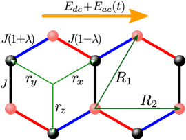
Figure 1: Kitaev model with (blue, red, black) $x$, $y$, $z$-bonds, hosting $S_{{\bf l}}^{\alpha}S_{{\bf l}+{\bf r}_{\alpha}}^{\alpha}$exchange with $\alpha{=}x$, $y$, $z$, respectively, in electric field $E_{dc}+E_{ac}(t)$ $\perp$ to $z$-bonds. $J\,[1+\lambda,1-\lambda,1$] refers to exchange interactions on $x$, $y$, $z$-bonds including dimerization $\lambda=-gE_{dc}$ by static field.

Following established literature [33, 35], Eqs. (1,2) map onto a quadratic forms of Majorana fermions in the presence of a static $\mathbb{Z}_{2}$ gauge $\eta_{{\bf l}}=\allowbreak\pm 1$, residing on, e.g., the $\alpha=\allowbreak z$ bonds

$$H_{0}-P(E_{dc}+E_{ac}(t))=H-PE_{ac}(t)s=$$ (3)

$$-\frac{i}{2}\!\sum_{{\bf l},\alpha=x,y,z}\!\!\!\!J_{\alpha}\eta_{{\bf l},\alpha}\,a_{{\bf l}}c_{{\bf l}+{\bf r}_{\alpha}}+\frac{i}{2}\!\sum_{{\bf l},\alpha=x,y}\!\!\!\!\mathrm{sg}_{\alpha}\,a_{{\bf l}}c_{{\bf l}+{\bf r}_{\alpha}}\,gE_{ac}(t)\,,$$

where $\eta_{{\bf l},x(y)}=1$, $\eta_{{\bf l},z}=\eta_{{\bf l}}$, and $\mathrm{sg}_{\alpha}=+(-)$ for $\alpha=x(y)$. There are two types of Majorana particles, corresponding to the two basis sites. We use the normalization $\{a_{{\bf l}},a_{{\bf l}^{\prime}}\}=\delta_{{\bf l},{\bf l}^{\prime}}$, $\{c_{{\bf m}},c_{{\bf m}^{\prime}}\}=\delta_{{\bf m},{\bf m}^{\prime}}$, and $\{a_{{\bf l}},c_{{\bf m}}\}=0$. Note that this Hamiltonian is diagonal in $\eta_{{\bf l},\alpha}$. I.e., the optical exchange-striction mechanism does not excite $\mathbb{Z}_{2}$ fluxes. For the remainder of this work $\hbar=k_{B}=1$.

III HH susceptibilities

In this section we detail the evaluation of the HH response functions. Two temperature regimes will be considered, namely $T\lesssim(\gtrsim)T^{\star}$, where $T^{\star}\approx 0.012\dotsc 0.025J$ is the so-called flux proliferation temperature. In a very narrow region of width $O(\pm 0.01J)$ centered around $T^{\star}$ the $\mathbb{Z}_{2}$-flux gets thermally populated, changing the average link density rapidly from $\langle\eta_{\mathbf{l}}\rangle=1$ to $\langle\eta_{\mathbf{l}}\rangle=0$ [70, 71, 72]. In the following, we will employ this and divide the temperature axis into approximately two regimes, i.e., the homogeneous flux sector in Sec. III.1 for $T\lesssim T^{\star}$ and the random flux sector [73] for $T\gtrsim T^{\star}$ in Sec. III.2. This approach has proven to work well on a quantitative level in several studies of the thermal conductivity of Kitaev models [71, 72, 74].

III.1 Higher harmonic susceptibilties below $T^{\star}$

For $\eta_{{\bf l}}=1$ the Hamiltonian (1) can be diagonalized analytically in terms of complex Dirac fermions. This procedure has been detailed extensively in various ways in the literature, e.g., [55, 75, 56, 35] and refs. therein. We merely state the quantities needed for the present calculations. The real Majorana fermions are mapped onto complex ones on half of the momentum space by Fourier transforming $a_{{\bf k}}^{\phantom{\dagger}}=\sum_{{\bf l}}e^{-i{\bf k}\cdot{\bf l}}a_{{\bf l}}/\sqrt{N}$ with momentum ${\bf k}$ and similarly for $c_{{\bf k}}^{\phantom{\dagger}}$. They satisfy $a_{{\bf k}}^{\dagger}=a_{-{\bf k}}^{\phantom{\dagger}}$. Standard anticommutation relations apply, $\{a_{{\bf k}}^{\phantom{\dagger}},\allowbreak a_{{\bf k}^{\prime}}^{\dagger}\}=\delta_{{\bf k},{\bf k}^{\prime}}$, $\{c_{{\bf k}}^{\phantom{\dagger}},\allowbreak c_{{\bf k}^{\prime}}^{\dagger}\}=\delta_{{\bf k},{\bf k}^{\prime}}$, and $\{a_{{\bf k}}^{(\dagger)}c_{{\bf k}^{\prime}}^{(\dagger)}\}=0$. The diagonal form of $H$ is

$$H=\tilde{\sum_{{\bf k},\gamma=1,2}}\mathrm{sg}_{\gamma}\,\epsilon_{{\bf k}}\,d_{\gamma{\bf k}}^{\dagger}d_{\gamma{\bf k}}^{\phantom{\dagger}}\,,$$ (4)

where $[c_{{\bf k}},a_{{\bf k}}]^{T}=\mathbf{u}(\mathbf{k})\,[d_{1{\bf k}},d_{2{\bf k}}]^{T}$ defines the quasiparticle fermions $d_{i{\bf k}}$ via a unitary transformation $\mathbf{u}(\mathbf{k})$, App. D, and $\mathrm{sg}_{\gamma}$=1(-1) for $\gamma$=1(2). The quasiparticles satisfy $\smash{d_{1(2){\bf k}}^{\dagger}=d_{2(1)-{\bf k}}^{\phantom{\dagger}}}$, and $\smash{\tilde{\sum}}$ sums over half of momentum space. In cartesian coordinates the quasiparticle energy $\epsilon_{{\bf k}}$ reads $\epsilon_{{\bf k}}=\allowbreak J[3+\allowbreak 2\lambda^{2}+\allowbreak 2(1-\lambda^{2})\cos(k_{x})+\allowbreak 4\cos(k_{x}/2)\allowbreak\cos(\sqrt{3}k_{y}/2)-\allowbreak 4\lambda\sin(k_{x}/2)\allowbreak\sin(\sqrt{3}k_{y}/2)]^{1/2}/2$.

Using the unitary trafo $\mathbf{u}(\mathbf{k})$, we may express $P$ in terms of the quasiparticle Dirac fermions

$$P=g\tilde{\sum_{{\bf k},\mu\nu}}d_{\mu{\bf k}}^{\dagger}p_{\mu\nu}(\mathbf{k})d_{\nu{\bf k}}^{\phantom{\dagger}}\,,$$ (5)

where, in cartesian coordinates, $p_{11}(\mathbf{k})=\allowbreak-p_{22}(\mathbf{k})=\allowbreak\sin(\allowbreak k_{x}/\allowbreak 2)\allowbreak(2\lambda\sin(k_{x}/2)-\allowbreak\sin(\sqrt{3}k_{y}/2))/\allowbreak(2\epsilon_{{\bf k}})$ and $p_{12}(\mathbf{k})=\allowbreak p_{21}^{\star}(\mathbf{k})=\allowbreak-i\sin(k_{x}/2)\allowbreak(2\cos(\allowbreak k_{x}/\allowbreak 2)+\allowbreak\cos(\allowbreak\sqrt{3}k_{y}/2))/\allowbreak(2\epsilon_{{\bf k}})$. Obviously $P$ is not diagonal in the quasiparticle basis, implying both, inter- and intraband excitations to occur.

Figure 2: Diagrams for $N$HG susceptibilities $\chi_{N\omega}(\omega)$ to leading order in $E_{ac}(t)$ for $N=1,2,3$.

Using Appendix A, we are now in a position to formulate the $N$th harmonic susceptibilities diagrammatically as in Fig. 2. For the AC field we use $E_{ac}(t)=(e^{i\omega t}+\allowbreak e^{-i\omega t})A$, with amplitude $A$. To appreciate these graphs, we first note, that in principle $N$th harmonics can arise from any combination of contributions by the field $\propto\exp[(\sum_{l}\pm 1_{l})it\omega]$, such that the sum of all signs of input frequencies satisfy $\sum_{l}\pm 1_{l}=N$. In turn $N$th harmonics can be generated at order $E_{ac}^{M}(t)$ with $M=N+2m$, $m\in\mathbb{N}$. For the remainder of this work we will consider only the leading order, i.e., $M=N$ [76]. Second, we emphasize that for the latter situation, the intrinsic permutation from Eq. (20) is the identity, i.e., only a single graph has to be considered for each $N$. Third, for all purposes the wave vector of the incoming light can be set to zero $\mathbf{q}=0$. Finally, for each Green’s function line in Fig. 2, two contributions $G_{\gamma}(\mathbf{k},\epsilon_{n})$ with $\gamma=1,2$ from the two quasiparticle bands arise, fixing also the matrix elements $p_{\mu\nu}(\mathbf{k})$ distributed along each graph.

Evaluation of the susceptibilities is straightforward. For Fig. 2(a)-(c) we obtain

$$\chi_{\omega}(\omega)= g^{2}\tilde{\sum_{\mathbf{k}}}\frac{4(2f_{\mathbf{k}}{-}1)\epsilon_{\mathbf{k}}\,|p_{12}(\mathbf{k})|^{2}}{(\omega_{+}^{2}-4\epsilon_{\mathbf{k}}^{2})}$$ (6)

$$\chi_{2\omega}(\omega)= g^{3}\tilde{\sum_{\mathbf{k}}}\frac{6(2f_{\mathbf{k}}{-}1)\epsilon_{\mathbf{k}}^{2}\,p_{11}(\mathbf{k})|p_{12}(\mathbf{k})|^{2}}{(\omega_{+}^{2}-\epsilon_{\mathbf{k}}^{2})(\omega_{+}^{2}-4\epsilon_{\mathbf{k}}^{2})}$$ (7)

$$\chi_{3\omega}(\omega)= g^{4}\tilde{\sum_{\mathbf{k}}}\left[\frac{8(2f_{\mathbf{k}}{-}1)|p_{12}(\mathbf{k})|^{2}\epsilon_{\mathbf{k}}}{(9\omega_{+}^{2}-4\epsilon_{\mathbf{k}}^{2})}\right.$$ (8)

$$\left.\times\frac{(|p_{12}(\mathbf{k})|^{2}(\omega_{+}^{2}-\epsilon_{\mathbf{k}}^{2})+p_{11}^{2}(\mathbf{k})(\omega_{+}^{2}+4\epsilon_{\mathbf{k}}^{2}))}{(\omega_{+}^{2}-\epsilon_{\mathbf{k}}^{2})(\omega_{+}^{2}-4\epsilon_{\mathbf{k}}^{2})}\right]\,.$$

Calculating the diagrams for $\chi_{N\omega}(\omega)$ can be cast into symbolic algebra code swiftly, providing analytical expressions with minimal resources, easily up to $N>10$ [77]. Therefore in practice, real-time HH response can be obtained for any input pulse shape without repetitive solutions of Lindblad-equations by convolution with analytic expressions for $\chi_{N\omega}(\omega)$.

The susceptibilities (6-8) display the resonance structure, typical of $N$HG. In particular, for each $N$, resonant enhancement occurs at integer fractions of $2\epsilon_{\mathbf{k}}$, down to $\omega=2\epsilon_{\mathbf{k}}/N$, indicative of the cooperative transition of $N$ photons of frequency $\omega$ at a fermion gap of $2\epsilon_{\mathbf{k}}$.

Not only the pure Kitaev model, but also its homogeneous flux sector satisfies the $U$-symmetry discussed in Sec. II. Indeed, following the diagrams of Fig. 2 and Eqs. (6-8), it is clear, that any even-$N$ harmonic susceptibility, including those at sub-leading order in $E_{ac}(t)$, contain an odd [even] power of $p_{11}(\mathbf{k})$ [$|p_{12}(\mathbf{k})|$]. Moreover, for vanishing static fields, i.e., $\lambda=0$, $\epsilon_{k_{x},k_{y}}=\allowbreak\epsilon_{-k_{x},k_{y}}$, $p_{11}(k_{x},k_{y})=\allowbreak-p_{11}(-k_{x},k_{y})$, and $|p_{12}(k_{x},k_{y})|=\allowbreak|p_{12}(-k_{x},k_{y})|$, as well as an identical relation for $k_{y}\rightarrow\allowbreak-k_{y}$. Therefore, at $\lambda=0$, all even-$N$ harmonic susceptibilities vanish. This agrees with Ref. [62].

III.2 Second harmonic susceptibilities above $T^{\star}$

In phases with random flux enclosed, i.e., for $T>T^{\star}$, Hamiltonian (3) loses translational invariance and we resort to a formulation amenable to numerical treatment in real space. This approach has been detailed in the literature [55, 75, 56]. We only list those points necessary to clarify the calculation of susceptibilities.

The Majorana fermions on the $2N$ sites in Eq. (3) are encoded into a spinor $A_{\text{$\sigma$}}^{\dagger}=(a_{1}\dots\allowbreak a_{{\bf l}}\dots\allowbreak a_{N},\allowbreak c_{1}\dots\allowbreak c_{{\bf l}+{\bf r}_{x}}\dots c_{N})$. This is mapped onto a spinor of complex Dirac fermions $D_{\sigma}^{\dagger}=(d_{1}^{\dagger}\dots d_{N}^{\dagger},d_{1}^{\phantom{\dagger}}\dots d_{N}^{\phantom{\dagger}})$ using a unitary (Fourier) transform ${\bf F}$. I.e., ${\bf D}={\bf F}{\bf A}$ where bold faced symbols refer to vectors or matrices. ${\bf F}$ is constructed from two disjoint $N\times N$ blocks $F_{\sigma\rho}^{i=1,2}=e^{-i{\bf k}_{\sigma}\cdot{\bf R}_{\rho}^{i}}/\sqrt{N}$, with $\sigma,\rho=1\dotsc N$ and ${\bf R}_{\rho}^{i}={\bf l}$ and ${\bf l}+{\bf r}_{x}$, for $a$- and $c$-Majorana lattice sites, respectively. $\mathbf{F}$ merely serves as a device to introduce complex fermions. ${\bf k}$ is chosen such, that for each ${\bf k}$, there exists one $-{\bf k}$, with ${\bf k}\neq-{\bf k}$. Finally, for convenience, ${\bf F}$ is rearranged such as to associate the $d_{1}^{\dagger}\dots d_{N}^{\dagger}$ with the $2\,(N/2)=N$ ’positive’ ${\bf k}$-vectors. In terms of these notations and for any set of values $\{\eta_{\mathbf{l}}\}$

$$H={\bf D}^{\dagger}{\bf h}\,{\bf D}/2\,,\hphantom{aaa}P=g\,{\bf D}^{\dagger}{\bf p}\,{\bf D}/2\,.\hphantom{aaa}$$ (9)

The $2N\times 2N$ matrices $\mathbf{h}$ and $\mathbf{p}$ are in general non-diagonal and contain particle number non-conserving terms. Finally, at this stage, and for a fixed distribution of $\{\eta_{\mathbf{l}}\}$ numerics is invoked to obtain a Bogoliubov transformation $\mathbf{U}$, diagonalizing $\mathbf{h}$, i.e., $({\bf U}\mathbf{h}{\bf U}^{\dagger})_{\rho\sigma}=\delta_{\rho\sigma}\epsilon_{\rho}$, with $\epsilon_{\rho}=(\epsilon_{1}\dots\epsilon_{N},-\epsilon_{1}\dots-\epsilon_{N})$ and quasiparticles ${\bf S}=\allowbreak{\bf U}{\bf D}$, for which $H=\sum_{\rho=1}^{2N}\epsilon_{\rho}S_{\rho}^{\dagger}S_{\rho}^{\phantom{\dagger}}/2$. We stay within a Nambu-notation with $\rho=1\dotsc 2N$, i.e., keeping the particle- and hole-range of $S_{\rho}^{(\dagger)}$, because the quasiparticle form of the polarization $P=g\,{\bf S}^{\dagger}{\bf m}\,{\bf S}/2$ is not simultaneously diagonal with $H$. It remains particle-number non-conserving.

The quasiparticle Green’s function $G_{\alpha\beta}(\tau)=-\langle T_{\tau}(S_{\alpha}^{\phantom{\dagger}}\allowbreak S_{\beta}^{\dagger})\rangle$ in Matsubara frequency space reads

$$G_{\alpha\beta}(\varepsilon_{n})=\delta_{\alpha\beta}G_{\alpha}(\varepsilon_{n})=\delta_{\alpha\beta}/(i\varepsilon_{n}-\epsilon_{\alpha})\,,$$ (10)

with $\varepsilon_{n}=(2n+1)\pi T$. To appreciate this textbook equation in the present context, we introduce a notation, connecting the particle- and hole-indices of $S_{\rho}$, namely $\bar{\rho}=\rho\mp N$ for $\rho\gtrless N$. With that, anomalous Green’s functions simply fulfill $-\langle T_{\tau}(S_{\alpha}^{\text{$\dagger$}}S_{\beta}^{\dagger})\rangle=-\langle T_{\tau}(S_{\bar{\alpha}}^{\phantom{\dagger}}S_{\beta}^{\dagger})\rangle=G_{\bar{\alpha}\beta}(\tau)$, with $\epsilon_{\bar{\alpha}}=-\epsilon_{\alpha}$. This renders normal and anomalous contractions in the diagrams of Fig. 2 straightforward, using Eq. (10) only and summing proper index combinations for the polarization vertices $m_{\alpha\beta}$. Diagram Fig. 2 (b) yields

$$\chi_{2i\omega_{n}}(i\omega_{n})=-g^{3}\,T\!\!\!\sum_{\alpha\beta\gamma,\varepsilon_{m}}[t_{\alpha\gamma}t_{\gamma\beta}t_{\beta\alpha}$$ (11)

$$\hphantom{aaaaaaa}\times G_{\alpha}(\varepsilon_{m}{+}2\omega_{n})G_{\beta}(\varepsilon_{m}{+}\omega_{n})G_{\gamma}(\varepsilon_{m})]\,,$$

with $t_{\alpha\beta}=(m_{\alpha\beta}-m_{\bar{\beta}\bar{\alpha}})/2$, where the first addend refers to the normal contraction order, and the second to the anomalous. Frequency summation and analytic continuation results in

$$\chi_{2\omega}(\omega)=g^{3}\sum_{\alpha\beta\gamma,\varepsilon_{m}} \frac{t_{\alpha\gamma}t_{\gamma\beta}t_{\beta\alpha}}{2\omega_{+}-\epsilon_{\alpha}+\epsilon_{\gamma}}\left(\frac{f_{\beta}-f_{\alpha}}{\omega_{+}-\epsilon_{\alpha}+\epsilon_{\beta}}+\right.$$

$$\left.\hphantom{aa}\frac{f_{\beta}-f_{\gamma}}{\omega_{+}-\epsilon_{\beta}+\epsilon_{\gamma}}\right)\,,$$ (12)

with the Fermi function $f_{\alpha}=1/(\exp(\epsilon_{\alpha}/T)+1)$. Obviously Eqs. (11,12) can readily be generalized to any HH susceptibility. We refrain from this.

To complete our evaluation of $\chi_{N\omega}(\omega)$ for $T\gtrsim T^{\star}$, a sufficiently large number of random distributions $\{\eta_{{\bf l}}\}$ is generated, for each of which $\mathbf{U}$, $\epsilon_{\alpha}$, $m_{\alpha\beta}$, and Eqs. (12) are calculated numerically, with a final average over all $\chi_{N\omega}(\omega)$ obtained [78].

IV Results and discussion

For the purpose of discussion and to highlight some of the results of this work, it seems of help to sketch the physics by elementary considerations on a two-level system. Since the homogeneous sector is translationally invariant, all HHG processes can be viewed as occurring on a disjoint collection of pairs of states $\{1\mathbf{k},2\mathbf{k}\}$ with energies $\{\epsilon_{\mathbf{k}},-\epsilon_{\mathbf{k}}\}$, enumerated by $\mathbf{k}$. For discussion, we reduce this to a single two-level Hamiltonian $H=\epsilon|1\rangle\langle 1|-\allowbreak\epsilon|2\rangle\langle 2|$, an accompanying polarization $P=n|1\rangle\langle 1|+\allowbreak m|2\rangle\langle 2|+\allowbreak g|1\rangle\langle 2|+\allowbreak g^{\star}|2\rangle\langle 1|$, and a driving field $E(t)=\allowbreak(e^{i\omega t}+\allowbreak e^{-i\omega t})A$, with a combined Hamiltonian of $H+P\,E(t)$. We are interested in the expectation value $\langle P\rangle_{\rho}(t)$, with respect to the time-dependent density matrix $\rho(t)$. In the interaction picture $\dot{\rho}(t)=\allowbreak-i[Q(t),\rho(t)]$, with $Q(t)=P(t)E(t)=e^{iHt}\allowbreak P\allowbreak e^{-iHt}\allowbreak E(t)=(n|1\rangle\langle 1|+\allowbreak m|2\rangle\langle 2|+\allowbreak ge^{2i\epsilon t}|1\rangle\langle 2|+\allowbreak g^{\star}e^{-2i\epsilon t}\allowbreak|2\rangle\langle 1|)\allowbreak E(t)$.

Without loss of generality, from the various commutator contributions to $\rho(t)$ for $2$HG, analogous to App. A, we pick a single time-ordering, with all $Q(t)$ left of $\rho_{0}$, the equilibrium density matrix at $t=-\infty$, set to the zero-temperature limit $\rho_{0}=|2\rangle\langle 2|$. Using only the $e^{-i\omega t}A$ component of the driving field for the purpose of $2$HG, the contribution reads

$$\rho_{2\omega}(t)=-A^{2} \int_{-\infty}^{t}dt_{1}\int_{-\infty}^{t_{1}}dt_{2}\,ne^{-i\omega_{+}t_{1}}\,|1\rangle\langle 1|\,\times$$ (13)

$$\hphantom{aa}ge^{-i(\omega_{+}-2\epsilon)t_{2}}\,|1\rangle\langle 2|\,|2\rangle\langle 2|+\dotsc$$

$$=A^{2} \,n\,g\,\frac{|1\rangle\langle 1|\,|1\rangle\langle 2|\,|2\rangle\langle 2|}{(2\omega_{+}-2\epsilon)(\omega_{+}-2\epsilon)}e^{-i(2\omega-2\epsilon)t}+\dotsc\,.$$

The selected time ordering shows off in the sequence of projectors $|\mu\rangle\langle\nu|$ and “$\dotsc$” refers to all orderings discarded. From this density matrix $\langle P\rangle_{\rho}(t)=\allowbreak A^{2}\allowbreak e^{-i2\omega_{+}t}\allowbreak n|g|^{2}/\allowbreak((2\omega_{+}-2\epsilon)(\omega_{+}-2\epsilon))$.

Obviously, $\langle P\rangle_{\rho}(t)$ displays frequency doubling. Moreover, the structure of matrix elements is consistent with Eq. (7), replacing $n|g|^{2}\leftrightarrow\allowbreak p_{11}(\mathbf{k})|p_{12}(\mathbf{k})|^{2}$. Finally, the sequence of projectors in the last line of Eq. (13) allows to interpret the resonance denominators: The first photon invokes an interband transition with resonance $(\omega-2\epsilon)^{-1}$. The second photon invokes an intraband transition with resonance $(2\omega-2\epsilon)^{-1}$. Connecting this with Eqs. (6-8), an $N$HG response function shows $N$ resonances, separated by fixed, coupled integer fractions of the two-level energy $\pm 2\epsilon_{\mathbf{k}}$, for each $\mathbf{k}$.

This physics is drastically altered by gauge disorder. It renders the Hamiltonian diagonal in a set of single fermion states, the quantum numbers of which will be completely mixed by the polarization operator. The consecutive absorption of $m{=}1{\dotsc}N$ photons of Eq. (13) remains intact, however, the corresponding resonance denominators $(m\omega_{+}-\epsilon_{\alpha}+\epsilon_{\beta})^{-1}$ are independently distributed over all energies, i.e., they are decoupled. The transitions may be intra- or interband, depending on the sign of $\epsilon_{\alpha}\epsilon_{\beta}$. This is the content of Eq. (12) in terms of the non-diagonal matrix elements $t_{\alpha\beta}$ and the resonance denominators.

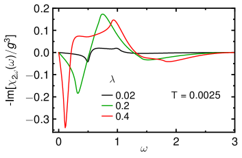
Figure 3: Imaginary part of dynamical $2$HG susceptibility in homogeneous gauge sector versus $\omega$, for various static fields $\lambda=-gE_{dc}$ at fixed temperature $T$. Linear system size $L{=}400$, imaginary broadening $0.01$, energies in units of $J$.

In the homogeneous gauge sector, summing over $\mathbf{k}$, the product structure of resonances of Eq. (13), comprising a sign change between the poles, and interlocked by a fixed energy ratio of $2$, can promote oscillations of $\mathrm{Im}\chi_{2\omega}(\omega)$, in addition to oscillations which are induced by $p_{11}(\mathbf{k})$. In random gauge sectors however, such oscillatory behavior should be suppressed, in particular towards lower frequencies, where resonance pairs from all energies overlap randomly.

To substantiate the preceding, we now discuss several plots of $\chi_{2\omega}(\omega)$. Fig. 3 displays the spectrum $\mathrm{Im}\chi_{2\omega}(\omega)$ from Eq. (7) at very low temperature $T=0.0025$ for various $gE_{dc}$. Since $\chi_{2\omega}(\omega)$ is holomorphic in the upper half plane, $\mathrm{Re}\chi_{2\omega}(\omega)$ follows from Kramers-Kronig and will not be shown henceforth. The figure exemplifies the 2HG selection rule, consistent with [62]. I.e., in the limit $gE_{dc}\rightarrow 0$ the susceptibility vanishes. $\chi_{2\omega}(\omega)$ is antisymmetric with respect to $gE_{dc}$. The spectrum clearly shows the oscillatory behavior discussed previously, exhibiting several sign changes within the range $0<\omega<2\mathrm{max}(\epsilon_{\mathbf{k}})=3J$. As is evident from the figure, the fermionic density-of-states modifications, due to $gE_{dc}$ lead to characteristic shifts of van-Hove structures in the spectrum. The values for $gE_{dc}$ in this figure are exploratory only. Its experimentally accessible range remains to be clarified.

Next, in Fig. 4, we consider the temperature dependence of the $2$HG susceptibility in the homogeneous gauge sector at a finite $gE_{dc}$. Two of the temperatures displayed, i.e., $T=0.25J$ and $0.5J$ are well above the flux proliferation crossover. Analyzing such temperatures with a homogeneous gauge is for demonstration only and serves the purpose of clarifying the impact of thermally excited flux later. The figure clearly shows the effect of the statistics of the fermions. I.e., as the temperature increases, interband excitations get blocked by thermal occupation, encoded by the factor $(1-2f_{\mathbf{k}})$ in Eqs. (6-8) for all HHG susceptibilities. This so-called Fermi-blocking has been highlighted as a fingerprint of fractionalization for a growing list of spectral probes of Kitaev magnets, including Raman scattering [51, 52, 53], resonant X-ray scattering [54], phonon spectra [55, 56, 57, 58, 59, 60], and ultrasound propagation [61]. As a main result, the present study adds HHG to this list.

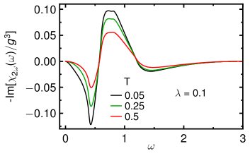
Figure 4: Imaginary part of dynamical $2$HG susceptibility in homogeneous gauge sector versus $\omega$, for various temperatures $T$ at fixed static field $\lambda=-gE_{dc}$. Linear system size $L{=}400$, imaginary broadening $0.01$, energies in units of $J$.

Fig. 5 displays the temperature dependence of the $2$HG susceptibility in the random gauge sector, at the same fixed static field, as in Fig. 4. First it should be noted, that the linear system size $L=30$ is considerably smaller than for the homogeneous sector. On the one hand, this is a prerequisite for acceptable runtimes of Eq. (12), comprising a Bogoliubov transform, a matrix-product trace for each $\omega$, and an average over $\{\eta_{\mathbf{l}}\}$ distributions. On the other hand, using $L\sim 30$ for a strictly homogeneous gauge is impractical, because of finite-size degeneracies. These are absent in the random gauge sector. Consequently, comparing $\chi_{2\omega}(\omega)$ between homogeneous and random sectors, some quantitative finite-size differences remain inevitable (see also App. C).

Apart from finite size effects, the spectra in Figs. 5 and 4 differ qualitatively. This difference can now be understood in terms of the discussion at the start of this section. I.e., in the random gauge sector the low- and high-frequency resonance energies from Eq. (12), $(\epsilon_{\alpha}-\epsilon_{\gamma})/2$ and $(\epsilon_{\alpha}-\epsilon_{\beta})$, $(\epsilon_{\beta}-\epsilon_{\gamma})$, respectively, are distributed independent and randomly, with a DOS that is almost flat [70] and they are coupled by non-diagonal matrix elements. This modifies the lower energy region of $\chi_{2\omega}(\omega)$, leading to significantly less oscillatory behavior as compared to Fig. 4. In addition to this qualitative difference, Fig. 5 shows Fermi-blocking similar to Fig. 4. Therefore, as another main result of this study, for $T\gtrsim T^{\star}$, both, the statistics of the fermionic quasiparticles, as well as the visons impact the $2$HG susceptibility.

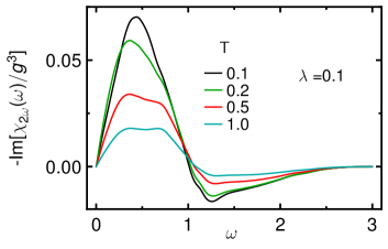
Figure 5: Imaginary part of dynamical $2$HG susceptibility in random gauge sector versus $\omega$, for various temperatures $T$ at fixed static field $\lambda=-gE_{dc}$. Linear system size $L{=}30$, number of random realizations $62$, imaginary broadening $0.05$, energies in units of $J$.

In Fig. 6 we approximate the evolution of the $2$HG susceptibility through the flux-proliferation crossover. An unbiased treatment of this requires evaluation of a dynamical 3-point correlation-function at intermediate flux density, varying the temperature across $T^{\star}$. Quantum Monte-Carlo [70] calculations for this is an open issue. For exact diagonalization [71] finite-size effects are expected to be detrimental. To make progress, we therefore resort to a phenomenological approach. This amounts to fixing a temperature $T\approx T^{\star}$, e.g., $T=0.05J$ and consecutively varying the average density $n_{\eta}$ of flipped gauge links from a low value, essentially describing the homogeneous flux sector, up to its maximum possible value at $n_{\eta}=1{/}2$. This provides for an approximate interpolation. Since flux proliferation occurs within a rather narrow temperature window of $O(T^{\star})\ll J$, varying the temperature of the fermions can be discarded. First, comparing the spectrum at $T=0.05$ in Fig. 4 with that for $n_{\eta}=0.05$ in Fig. 6 provides a rough measure for the finite size differences between $L=400$ and $30$. Otherwise, these spectra show the same oscillatory behavior, representative of the homogeneous sector. Using exactly $n_{\eta}=0$ within the $\mathbf{r}$-space code is inconvenient because of large degeneracies at $L=30$. Remarkably, and as another main result, Fig. 6 corroborates the discussion at the start of this section. I.e., the low-energy modulations of $\chi_{2\omega}(\omega)$ are continuously removed as $n_{\eta}$ increases. Quantitatively, the high energy spectrum is less affected by the increase of flux-density.

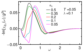
Figure 6: Imaginary part of dynamical $2$HG susceptibility versus $\omega$, for various flipped gauge link densities at fixed temperature $T{=}0.05{\sim}T^{\star}$ and static field $\lambda=-gE_{dc}$. Linear system size $L{=}30$, number of random realizations $62$, imaginary broadening $0.05$, energies in units of $J$.

Finally, we show results for the dc-field dependence of $\chi_{2\omega}(\omega)$ in the random gauge sector in Fig. 7. While for a single gauge sector with a fixed random distribution of $\eta_{\mathbf{l}}$, the $U$-symmetry of Sec. II will not be satisfied in general, it is mandatory that after averaging over random $\eta_{\mathbf{l}}$ distributions, to within the statistical error $\chi_{2\omega}(\omega)$ must vanish for vanishing $gE_{dc}$, in order to encode the physics of the pure Kitaev model. Fig. 7 clearly evidences this behavior, implying that the pure Kitaev magnet shows no $2$HG at any temperature.

V Summary

We have studied finite temperature $2$HG in the Kitaev magnet. We found that fractionalization in this frustrated quantum spin system has a profound impact on the evolution of the 2HG susceptibility with temperature. Mobile fermionic excitations, which are one kind of fractional quasiparticles of this system, lead to an overall reduction of HHG susceptibilities by Fermi-blocking on a temperature scale of the exchange coupling constant. This is in line with other spectroscopic probes of the Kitaev magnet. In addition however, a second low-temperature scale $T^{\star}$ exists, in the narrow vicinity of which localized $\mathbb{Z}_{2}$ visons, which are the second kind of fractional quasiparticles, are thermally populated. This induces strong qualitative changes of the 2HG susceptibility, by smoothing spectral oscillations up to intermediate energies. In turn, both types of fractional quasiparticles play an important role in finite temperature 2HG. While we have analyzed the effects of the visons on the 2HG only, it is tempting to suggest that this physics applies to all HHG.

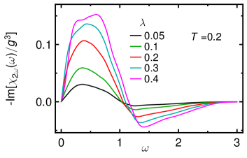
Figure 7: Imaginary part of dynamical $2$HG susceptibility in random gauge sector versus $\omega$, for various static fields $\lambda=-gE_{dc}$ at fixed temperature $T$. Linear system size $L{=}30$, number of random realizations $62$, imaginary broadening $0.05$, energies in units of $J$.

Speculating on experimental consequences for the proximate Kitaev magnet $\alpha$-RuCl₃, it should be realized first, that full access to the conclusions of this work would be possible only in the potential QSL phase in the in-plane field range of $H{\parallel}a\sim 7{\dotsc}9$T. Second, since $J\sim 90K$ is in the terahertz range, the response of convoluting few-cycle terahertz pulses with the 2HG susceptibility should be very sensitive to the drastic changes between Figs. 4 and 5. Therefore, apart from the gradual intensity increase on a scale of $\sim 90K$ by Fermi-blocking as $T$ is lowered, a vison-induced strong intensity change should occur for $T\sim 1\dotsc 5K$. Finally, the even HG selection rule seems an interesting case where strain experiments could be of interest.

Our considerations have left aside the role of static magnetic fields $H$ for the fermions and visons. For the former, magnetic field induced gaps are low-energy features only and are smeared out by vison disorder for $T>T^{\star}$. For the latter, vison dispersion generated by magnetic fields could lead to interesting phenomena, which are beyond the scope of this study.

Finally we note, that the methods described in this work are directly applicable to the analysis of other types of higher order spectroscopies in Kitaev magnets [83].

Appendix A $n$th order response diagrams

Let

$$H(t)=H-P\,E(t)\,,$$ (14)

be a time dependent Hamiltonian. For labeling purpose, $P$ is dubbed a “polarization” and $E(t)$ a time-dependent “electric field”. We assume the electric field to be adiabatically switched on, starting at $t=-\infty$. The response at time $t$ of $P$ to the perturbation $P\,E(t)$ is obtained from expanding the time-dependent density matrix $\rho(t)$ in the interaction picture [79]

$$\langle P\rangle(t)= \langle P\rangle+i\int_{-\infty}^{t}\langle[P(t),P(t_{1})]\rangle E(t_{1})\,dt_{1}+i^{2}\int_{-\infty}^{t}\int_{-\infty}^{t_{1}}\langle[[P(t),P(t_{1})],P(t_{2})]\rangle E(t_{1})E(t_{2})\,dt_{1}dt_{2}$$

$$+i^{n}\int_{-\infty}^{t}\dots\int_{-\infty}^{t_{n}}\langle[\dots[P(t),P(t_{1})],\dots,P(t_{n})]\rangle E(t_{1})\dots E(t_{n})\,dt_{1}\dots dt_{n}+\dotsc\,,$$ (15)

where $P(t)=e^{iHt}Pe^{-iHt}$ is the time dependence within the interaction picture. Eq.(15) can be written in terms of retarded susceptibilities

$$\Delta\langle P\rangle(t)= \int_{-\infty}^{\infty}\chi(t,t_{1})\,E(t_{1})\,dt_{1}+\int_{-\infty}^{\infty}\int_{-\infty}^{\infty}\chi(t,t_{1},t_{2})\,E(t_{1})E(t_{2})\,dt_{1}dt_{2}+\dots$$

$$+\int_{-\infty}^{\infty}\dots\int_{-\infty}^{\infty}\chi(t,t_{1},\dots,t_{2})\,E(t_{1})\dots E(t_{n})\,dt_{1}\dots dt_{n}+\dotsc$$ (16)

where

$$\chi(t,t_{1})= i\Theta(t-t_{1})\langle[P(t),P(t_{1})]\rangle\,,$$ (17)

$$\chi(t,t_{1},t_{2})= i^{2}\Theta(t-t_{1})\Theta(t_{1}-t_{2})\langle[[P(t),P(t_{1})],P(t_{2})]\rangle\,,$$ (18)

$$\chi(t,t_{1},t_{2},\dotsc,t_{n})= i^{n}\Theta(t-t_{1})\Theta(t_{1}-t_{2})\dotsc\Theta(t_{n-1}-t_{n})\langle[\dots[P(t),P(t_{1})],\dotsc,P(t_{n})]\rangle$$ (19)

$\chi(t,t_{1})$ is the standard 2-point linear response susceptibility. As usual, since $H$ is time-independent, $\langle[P(t),\allowbreak P(t_{1})]\rangle$ can be recast into $\langle[P(t-t_{1}),P]\rangle$, highlighting the dependence of $\chi(t,t_{1})$ on $t-t_{1}$.

All of the $n$-fold time integrations in Eq. (16) are totally symmetric with respect to any permutation of the $n$ time arguments. Therefore, all contributions to $\Delta\langle P\rangle(t)$ can be accounted for by replacing all susceptibilities by their fully symmetric part, dubbed intrinsic permutation symmetry [80]

$$\chi(t,t_{1},\dots,t_{n})\rightarrow\chi_{S}(t,t_{1},\dots,t_{n})$$

$$\phantom{aaaa}=\frac{1}{n!}\sum_{\pi}\chi(t,t_{\pi(1)},\dots,t_{\pi(n)})\,,$$ (20)

where $\pi$ labels all permutations.

It is textbook knowledge [79], that the Fourier transform $\chi(\omega)$ at real frequencies $\omega$ of the retarted 2-point function $\chi(t)=i\Theta(t)\langle[P(t),P]\rangle$ can be obtained from the Fourier transform of the imaginary time 2-point function $\chi(\tau)=\langle T_{\tau}(P(\tau)P)\rangle$ at Matsubara frequencies $i\omega_{n}=i\,2\pi T\,n$ by analytic continuation onto the real axis with $i\omega_{n}\rightarrow\omega+i0^{+}$. Beyond this however, the analytic continuation procedure applies to the evaluation of any fully symmetrized retarded $n$-point functions of an interacting systems for all $n$, including the case of arbitrary vertex operators, $P,P(t_{1}),\dots,P(t_{n-1})\rightarrow P_{0},P_{1}(t_{1}),\dots,P_{n-1}(t_{n-1})$ with $P_{i}\neq P_{j}$ for $i\neq j$. This has been proved in Refs. [81, 82]. Therefore, if $P$ can be expressed in terms of Fermions/Bosons, standard diagrammatic methods can be applied to calculate $\chi(t,t_{1},\allowbreak\dots,\allowbreak t_{n})$ for any $n$.

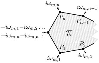
Figure 8: Intrinsically symmetrized $n+1$ point susceptibility.

Specifically, if $P$ is a quadratic form of Fermions/ Bosons, the preceding implies the diagram Fig. 8 for the $n+\allowbreak 1$ point susceptibility. Thick lines connecting the vertices $P_{j}$ refer to one-particle Green’s functions and the hatched background implies, that any kind of interactions may dress the graph, if $H$ provides for such. Finally, $\pi$ refers to an implicit sum over all such graphs with the vertices $i\omega_{m,j}\allowbreak P_{j}$ permuted along the outer lines of the diagram. This clarifies the correlation functions evaluated in Sec. III.1.

Appendix B Equation of motion approach

For an approach alternative to the diagrams in Fig. 2, one can also evaluate the commutators in Eq. (15) directly using the time dependent polarization operators within the interaction picture. In the $\mathbf{k}$-space formulation for the homogeneous state Eqs. (4,5) yield

$$P(t)=g\tilde{\sum_{{\bf k},\mu\nu}}e^{i(\epsilon_{\mu{\bf k}}-\epsilon_{\nu{\bf k}})t}d_{\mu{\bf k}}^{\dagger}p_{\mu\nu}(\mathbf{k})d_{\nu{\bf k}}^{\phantom{\dagger}}\,,$$ (21)

where $\epsilon_{\mu{\bf k}}=\mathrm{sg}_{\mu}\epsilon_{k}$, with $\mathrm{sg}_{\mu}$ as defined after Eq. (4). Inserting this into the commutators of Eq. (18) we get

$$\langle[[P(t),P(t_{1})],P(t_{2})]\rangle=$$

$$\hphantom{aaa}g^{3}\tilde{\sum_{{\bf k}}}2p_{11}(\mathbf{k})|p_{12}(\mathbf{k})|^{2}(e^{i2\epsilon_{{\bf k}}(t_{1}-t_{2})}-e^{i2\epsilon_{{\bf k}}(t-t_{2})}+$$

$$\hphantom{aaaaaaaaaa}e^{i2\epsilon_{{\bf k}}(t_{2}-t_{1})}-e^{i2\epsilon_{{\bf k}}(t_{2}-t)})(1-2f_{\mathbf{k}})\,,$$ (22)

where the Fermi function $f_{\mathbf{k}}$, defined after Eq. (8), results from thermal traces of type $\langle d_{\mu{\bf k}}^{\dagger}d_{\nu{\bf k}}^{\phantom{\dagger}}\rangle=\delta_{\mu\nu}\langle d_{\mu{\bf k}}^{\dagger}d_{\mu{\bf k}}^{\phantom{\dagger}}\rangle$. Since $P(t)$ is quadratic in the fermions, all thermal traces in Eq. (22) are also. Inserting Eq. (22) into the $O(E^{2})$ addend of Eq. (15) using $E(t)=Ae^{-i\omega_{+}t}$ in order to obtain the 2HG response, we arrive at $\chi_{2\omega}(\omega)$ identical to Eq. (7). Completely analogous, following the notation used in III.2, the polarization expressed in the interaction picture and in $\mathbf{r}$-space reads

$$P(t)=\frac{g}{2}\sum_{\mu\nu}e^{i(\epsilon_{\mu}-\epsilon_{\nu})t}S_{\mu}^{+}m_{\mu\nu}S_{\nu}\,,$$ (23)

where $\epsilon_{\mu}=(\epsilon_{1}\dots\epsilon_{N},-\epsilon_{1}\dots-\epsilon_{N})$ and $m_{\mu\nu}$ are matrix elements of $\mathbf{m}$, as defined after Eq. (9). Again, inserting this into the commutators of Eq. (18) we get

$$\langle[[P(t),P(t_{1})],P(t_{2})]\rangle=g^{3}\sum_{\alpha\beta\gamma}t_{\alpha\gamma}t_{\gamma\beta}t_{\beta\alpha}\times$$

$$\hphantom{aaaa}\left(e^{i(\epsilon_{\gamma}-\epsilon_{\alpha})t}e^{i(\epsilon_{\beta}-\epsilon_{\gamma})t_{1}}e^{i(\epsilon_{\alpha}-\epsilon_{\beta})t_{2}}(f_{\beta}-f_{\alpha})+\right.$$

$$\hphantom{aaaa}\left.e^{i(\epsilon_{\gamma}-\epsilon_{\alpha})t}e^{i(\epsilon_{\alpha}-\epsilon_{\beta})t_{1}}e^{i(\epsilon_{\beta}-\epsilon_{\gamma})t_{2}}(f_{\beta}-f_{\gamma})\right)\,,$$ (24)

where $t_{\alpha\beta}$ are defined after Eq. (11). Performing the integrations in Eq. (15) similar to the $\mathbf{k}$-space case, we arrive at $\chi_{2\omega}(\omega)$ identical to Eq. (12).

Appendix C Real space versus momentum space calculations

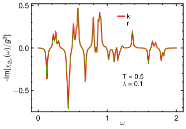
Figure 9: Section of imaginary part of dynamical $2$HG susceptibility on very small system of linear size $L{=}8$, comparing Eq. (7) (bold red) with fully numerical results from Eq. (12), forcing a homogeneous gauge (thin green) and setting imaginary broadening $0.01$ to resolve single quasiparticle poles. Energies in units of $J$.

This section is merely meant to prove numerically, that the two rather diametric approaches used in Sec. III.1 and Sec. III.2, i.e., the $\mathbf{k}$-space and $\mathbf{r}$-space calculations, indeed yield identical results if used within the translationally invariant, homogeneous gauge sector. For that purpose, we consider a system, deliberately chosen small enough to resolve single quasiparticle energies for a sufficiently small imaginary broadening and set the temperature such as to involve both, positive and negative quasiparticle energies. For such a case, we contrast $\mathrm{Im}\chi_{2\omega}(\omega)$ resulting from the analytical expressions Eq. (7) with that obtained from the fully numerical procedure in $\mathbf{r}$-space. A typical example is shown in Fig. 9. The results are identical to within numerical precision.

Appendix D Diagonalization of homogeneous sector

Here, for completeness sake, we list the unitary transformation to quasiparticles $\mathbf{u}(\mathbf{k})$, cited after Eq. (4) and known from the literature, e.g. [55]. The quasiparticles are given by

$$\left[\begin{array}[]{c}c_{{\bf k}}\\ a_{{\bf k}}\end{array}\right] =\left[\begin{array}[]{cc}u_{11}({\bf k})&u_{12}({\bf k})\\ u_{21}({\bf k})&u_{22}({\bf k})\end{array}\right]\left[\begin{array}[]{c}d_{1{\bf k}}\\ d_{2{\bf k}}\end{array}\right]$$ (31)

$$u_{11}({\bf k}) =-u_{12}({\bf k})=\frac{i\sum_{\alpha}e^{-i{\bf k}\cdot{\bf r}_{\alpha}}}{2^{3/2}\epsilon_{{\bf k}}}$$

$$u_{21}({\bf k}) =u_{22}({\bf k})=\frac{1}{\sqrt{2}}\,,$$

where the momontum $\mathbf{k}$ is set by ${\bf k}=x\,{\bf G}_{1}+y\,{\bf G}_{2}$ with $x,y\in[0,2\pi[$, in terms of the basis ${\bf G}_{1[2]}=(1,-\frac{1}{\sqrt{3}})\,[(0,\frac{2}{\sqrt{3}})]$, which is reciprocal to the triangular lattice basis listed after Eq. (1).

In terms of the reciprocal coordinates $x,y$, the quasiparticle energy $\epsilon_{{\bf k}}$ stated after Eq. (4) reads $\epsilon_{{\bf k}}=J[3+2\lambda^{2}+\allowbreak 2(1-\lambda^{2})\cos(x)+\allowbreak 2(1-\lambda)\cos(x-y)+\allowbreak 2(1+\lambda)\cos(y)]^{1/2}/2$.

Furthermore, the matrix elements of the dipole operator, cited after Eq. (5), in reciprocal coordinates are $p_{11}(\mathbf{k})=-p_{22}(\mathbf{k})=(\cos(y)-\allowbreak\cos(x-y)+\allowbreak 2\lambda(1-\allowbreak\cos(x)))/\allowbreak(4\epsilon_{{\bf k}})$ and $p_{12}(\mathbf{k})=p_{21}^{\star}(\mathbf{k})=-i(\sin(x-\allowbreak y)+\allowbreak 2\sin(x)+\allowbreak\sin(y))/\allowbreak(4\epsilon_{{\bf k}})$.

References

- [1] R. W. , Nonlinear Optics, 3rd ed. (Academic Press, Inc., Orlando, 2008).
- [2] M. Tokman, S. B. Bodrov, Y. A. Sergeev, A. I. Korytin, I. Oladyshkin, Y. Wang, A. Belyanin, and A. N. Stepanov, Phys. Rev. B 99, 155411 (2019).
- [3] M. Vandelli, M. I. Katsnelson, and E. A. Stepanov, Phys. Rev. B 99, 165432 (2019).
- [4] T. N. Ikeda, Phys. Rev. Research 2, 032015 (2020).
- [5] M. Zhang, N. Han, J. Wang, Z. Zhang, K. Liu, Z. Sun, J. Zhao, and X. Gan, Nano Lett. 22, 4287 (2022).
- [6] C. Janisch, Y. Wang, D. Ma, N. Mehta, A. L. Elías, N. Perea-López, M. Terrones, V. Crespi, and Z. Liu, Sci Rep 4, 5530 (2014).
- [7] H. G. Rosa, Y. Wei Ho, I. Verzhbitskiy, M. J. F. L. Rodrigues, T. Taniguchi, K. Watanabe, G. Eda, V. M. Pereira, and J. C. V. Gomes, Sci. Rep. 8, 10035 (2018).
- [8] Y. W. Ho, H. G. Rosa, I. Verzhbitskiy, M. J. L. F. Rodrigues, T. Taniguchi, K. Watanabe, G. Eda, V. M. Pereira, and J. C. Viana-Gomes, ACS Photonics 7, 925 (2020).
- [9] J. Yu, X. Kuang, J. Li, J. Zhong, C. Zeng, L. Cao, Z. Liu, Z. Zeng, Z. Luo, T. He, A. Pan, and Y. Liu, Nat Commun 12, 1083 (2021).
- [10] L. Mouchliadis, S. Psilodimitrakopoulos, G. M. Maragkakis, I. Demeridou, G. Kourmoulakis, A. Lemonis, G. Kioseoglou, and E. Stratakis, Npj 2D Mater Appl 5, 6 (2021).
- [11] L. Wu, S. Patankar, T. Morimoto, N. L. Nair, E. Thewalt, A. Little, J. G. Analytis, J. E. Moore, and J. Orenstein, Nature Phys 13, 350 (2017).
- [12] A. Abulikemu, Y. Kainuma, T. An, and M. Hase, ACS Photonics 8, 988 (2021).
- [13] R. von Baltz and W. Kraut, Phys. Rev. B 23, 5590 (1981).
- [14] A. M. Cook, B. M. Fregoso, F. de Juan, S. Coh, and J. E. Moore, Nat Commun 8, 14176 (2017).
- [15] L. Z. Tan and A. M. Rappe, Phys. Rev. Lett. 116, 237402 (2016).
- [16] H. Ishizuka and M. Sato, Phys. Rev. Lett. 129, 107201 (2022).
- [17] [1] O. E. Alon, V. Averbukh, and N. Moiseyev, Phys. Rev. Lett. 80, 3743 (1998).
- [18] T. Morimoto, H. C. Po, and A. Vishwanath, Phys. Rev. B 95, 195155 (2017).
- [19] O. Neufeld, D. Podolsky, and O. Cohen, Nat Commun 10, 405 (2019).
- [20] F. Ceccherini, D. Bauer, and F. Cornolti, J. Phys. B: At. Mol. Opt. Phys. 34, 5017 (2001).
- [21] B. M. Fregoso, Y. H. Wang, N. Gedik, and V. Galitski, Phys. Rev. B 88, 155129 (2013).
- [22] W. Kuehn, K. Reimann, M. Woerner, and T. Elsaesser, The Journal of Chemical Physics 130, 164503 (2009).
- [23] W. Kuehn, K. Reimann, M. Woerner, T. Elsaesser, and R. Hey, J. Phys. Chem. B 115, 5448 (2011).
- [24] G. S. Engel, T. R. Calhoun, E. L. Read, T.-K. Ahn, T. Mančal, Y.-C. Cheng, R. E. Blankenship, and G. R. Fleming, Nature 446, 782 (2007).
- [25] F. Mahmood, D. Chaudhuri, S. Gopalakrishnan, R. Nandkishore, and N. P. Armitage, Nat. Phys. 17, 627 (2021).
- [26] J. Lu, X. Li, H. Y. Hwang, B. K. Ofori-Okai, T. Kurihara, T. Suemoto, and K. A. Nelson, Phys. Rev. Lett. 118, 207204 (2017).
- [27] Y. Wan and N. P. Armitage, Phys. Rev. Lett. 122, 257401 (2019).
- [28] Z.-L. Li, M. Oshikawa, and Y. Wan, Phys. Rev. X 11, 031035 (2021).
- [29] R. M. Nandkishore, W. Choi, and Y. B. Kim, Phys. Rev. Research 3, 013254 (2021).
- [30] W. Choi, K. H. Lee, and Y. B. Kim, Phys. Rev. Lett. 124, 117205 (2020).
- [31] Y. Qiang, V. L. Quito, T. V. Trevisan, and P. P. Orth, arXiv:2301.11243.
- [32] L. Savary and L. Balents, Rep. Prog. Phys. 80, 016502 (2016).
- [33] A. Kitaev, Annals of Physics 321, 2 (2006).
- [34] H. Takagi, T. Takayama, G. Jackeli, G. Khaliullin, and S. E. Nagler, Nat Rev Phys 1, 264 (2019).
- [35] Y. Motome and J. Nasu, J. Phys. Soc. Jpn. 89, 012002 (2019).
- [36] G. Jackeli and G. Khaliullin, Phys. Rev. Lett. 102, 017205 (2009).
- [37] G. Baskaran, S. Mandal, and R. Shankar, Phys. Rev. Lett. 98, 247201 (2007).
- [38] K. W. Plumb, J. P. Clancy, L. J. Sandilands, V. V. Shankar, Y. F. Hu, K. S. Burch, H.-Y. Kee, and Y.-J. Kim, Phys. Rev. B 90, 041112 (2014).
- [39] H. B. Cao, A. Banerjee, J.-Q. Yan, C. A. Bridges, M. D. Lumsden, D. G. Mandrus, D. A. Tennant, B. C. Chakoumakos, and S. E. Nagler, Phys. Rev. B 93, 134423 (2016).
- [40] J. A. Sears, Y. Zhao, Z. Xu, J. W. Lynn, and Y.-J. Kim, Phys. Rev. B 95, 180411 (2017).
- [41] A. U. B. Wolter, L. T. Corredor, L. Janssen, K. Nenkov, S. Schönecker, S.-H. Do, K.-Y. Choi, R. Albrecht, J. Hunger, T. Doert, M. Vojta, and B. Büchner, Phys. Rev. B 96, 041405 (2017).
- [42] S.-H. Baek, S.-H. Do, K.-Y. Choi, Y. S. Kwon, A. U. B. Wolter, S. Nishimoto, J. van den Brink, and B. Büchner, Phys. Rev. Lett. 119, 037201 (2017)
- [43] R. Hentrich, A. U. B. Wolter, X. Zotos, W. Brenig, D. Nowak, A. Isaeva, T. Doert, A. Banerjee, P. Lampen-Kelley, D. G. Mandrus, S. E. Nagler, J. Sears, Y.-J. Kim, B. Büchner, and C. Hess, Phys. Rev. Lett. 120, 117204 (2018).
- [44] C. Balz, P. Lampen-Kelley, A. Banerjee, J. Yan, Z. Lu, X. Hu, S. M. Yadav, Y. Takano, Y. Liu, D. A. Tennant, M. D. Lumsden, D. Mandrus, and S. E. Nagler, Phys. Rev. B 100, 060405 (2019).
- [45] R. Schönemann, S. Imajo, F. Weickert, J. Yan, D. G. Mandrus, Y. Takano, E. L. Brosha, P. F. S. Rosa, S. E. Nagler, K. Kindo, and M. Jaime, Phys. Rev. B 102, 214432 (2020).
- [46] C. Balz, L. Janssen, P. Lampen-Kelley, A. Banerjee, Y. H. Liu, J.-Q. Yan, D. G. Mandrus, M. Vojta, and S. E. Nagler, Phys. Rev. B 103, 174417 (2021).
- [47] J. Knolle, D. L. Kovrizhin, J. T. Chalker, and R. Moessner, Phys. Rev. Lett. 112, 207203 (2014).
- [48] [1] A. Banerjee, C. A. Bridges, J.-Q. Yan, A. A. Aczel, L. Li, M. B. Stone, G. E. Granroth, M. D. Lumsden, Y. Yiu, J. Knolle, S. Bhattacharjee, D. L. Kovrizhin, R. Moessner, D. A. Tennant, D. G. Mandrus, and S. E. Nagler, Nature Materials 15, 733 (2016).
- [49] A. Banerjee, J. Yan, J. Knolle, C. A. Bridges, M. B. Stone, M. D. Lumsden, D. G. Mandrus, D. A. Tennant, R. Moessner, and S. E. Nagler, Science 356, 1055 (2017).
- [50] S.-H. Do, S.-Y. Park, J. Yoshitake, J. Nasu, Y. Motome, Y. S. Kwon, D. T. Adroja, D. J. Voneshen, K. Kim, T.-H. Jang, J.-H. Park, K.-Y. Choi, and S. Ji, Nature Phys 13, 1079 (2017).
- [51] L. J. Sandilands, Y. Tian, K. W. Plumb, Y.-J. Kim, and K. S. Burch, Phys. Rev. Lett. 114, 147201 (2015).
- [52] J. Nasu, J. Knolle, D. L. Kovrizhin, Y. Motome, and R. Moessner, Nature Physics 12, 912 (2016).
- [53] D. Wulferding, Y. Choi, S.-H. Do, C. H. Lee, P. Lemmens, C. Faugeras, Y. Gallais, and K.-Y. Choi, Nat Commun 11, 1 (2020).
- [54] G. B. Halász, N. B. Perkins, and J. van den Brink, Phys. Rev. Lett. 117, 127203 (2016).
- [55] A. Metavitsiadis and W. Brenig, Phys. Rev. B 101, 035103 (2020).
- [56] A. Metavitsiadis, W. Natori, J. Knolle, and W. Brenig, Phys. Rev. B 105, 165151 (2022).
- [57] M. Ye, R. M. Fernandes, and N. B. Perkins, Phys. Rev. Research 2, 033180 (2020).
- [58] K. Feng, M. Ye, and N. B. Perkins, Phys. Rev. B 103, 214416 (2021).
- [59] K. Feng, S. Swarup, and N. B. Perkins, Phys. Rev. B 105, L121108 (2022).
- [60] H. Li, T. T. Zhang, A. Said, G. Fabbris, D. G. Mazzone, J. Q. Yan, D. Mandrus, G. B. Halász, S. Okamoto, S. Murakami, M. P. M. Dean, H. N. Lee, and H. Miao, Nat Commun 12, 3513 (2021).
- [61] A. Hauspurg, S. Zherlitsyn, T. Helm, V. Felea, J. Wosnitza, V. Tsurkan, K.-Y. Choi, S.-H. Do, M. Ye, W. Brenig, and N. B. Perkins, arXiv:2303.09288.
- [62] M. Kanega, T. N. Ikeda, and M. Sato, Phys. Rev. Research 3, L032024 (2021).
- [63] H. Katsura, M. Sato, T. Furuta, and N. Nagaosa, Phys. Rev. Lett. 103, 177402 (2009).
- [64] J. Lorenzana and G. A. Sawatzky, Phys. Rev. Lett. 74, 1867 (1995).
- [65] C. Jurecka and W. Brenig Phys. Rev. B 61, 14307 (2000).
- [66] Y. Tokura, S. Seki, and N. Nagaosa, Rep. Prog. Phys. 77, 076501 (2014).
- [67] Generalizing field directions is postponed to future work.
- [68] O. A. Aktsipetrov, A. A. Fedyanin, E. D. Mishina, A. N. Rubtsov, C. W. van Hasselt, M. A. C. Devillers, and Th. Rasing, Phys. Rev. B 54, 1825 (1996).
- [69] A. Y. Bykov, T. V. Murzina, M. G. Rybin, and E. D. Obraztsova, Phys. Rev. B 85, 121413 (2012).
- [70] J. Nasu, M. Udagawa, and Y. Motome, Phys. Rev. B 92, 115122 (2015).
- [71] A. Metavitsiadis, A. Pidatella, and W. Brenig, Phys. Rev. B 96, 205121 (2017).
- [72] A. Pidatella, A. Metavitsiadis, and W. Brenig Phys. Rev. B 99, 075141 (2019).
- [73] The term “random flux sector” is used to imply an average over sectors with fixed, random values of .
- [74] A. Metavitsiadis and W. Brenig, Rev. B 96, 041115(R) (2017).
- [75] A. Metavitsiadis and W. Brenig, Phys. Rev. B 104, 104424 (2021).
- [76] This is merely for simplicity. No conceptual or technical reason prevents inclusion of graphs beyond the leading order in , at the expense of increasing the length of the analytical expressions.
- [77] Upon reasonable request, for will be provided in private communication.
- [78] The relative orientation of the polarization in Eq. (2) and the gauge-fixing on the -bonds does not imply unphysical anisotropies. This is satisfied by our -space code. I.e. the spectra we obtain in the random gauge sector are independent of pointing perpendicular to the , , or bonds.
- [79] A. L. Fetter and J. D. Walecka, Quantum Theory of Many-Particle Systems, McGraw-Hill, Boston, (1971)
- [80] P. N. Butcher, D. Cotter, The Elements of Nonlinear Optics, Cambridge University Press, Cambridge, 1990.
- [81] W. A. B. Evans, Proc. Phys. Soc. 88, 723 (1966).
- [82] H. Rostami, M. I. Katsnelson, G. Vignale, and M. Polini, Annals of Physics 431, 168523 (2021).
- [83] W. Brenig, unpublished.