Boundary to bound dictionary for generic Kerr orbits

Abstract

We establish a new relation between classical observables for scattering and bound orbits of a massive probe particle in a Kerr background. We find an exact representation of the Hamilton-Jacobi action in terms of the conserved charges which admits an analytic continuation, both for the radial and polar contribution, for a general class of geodesics beyond the equatorial case. Remarkably, this allows to extend the boundary to bound dictionary and it provides an efficient method to compute the deflection angles and the time delay for scattering orbits, as well as frequency ratios for bound orbits, in the probe limit but at all orders in the perturbative expansion.

I Introduction

The existence of gravitational waves was predicted by Einstein’s theory of general relativity (GR) in 1916, but it took until 2015 for the Laser Interferometer Gravitational-Wave Observatory (LIGO) to detect the first direct evidence of these elusive waves [1]. Since then, LIGO and other gravitational wave observatories around the world have detected numerous events, opening a new way to study the universe and test fundamental physics.

To accurately predict the properties of gravitational waves, a theoretical framework is required. One such framework is the post-Minkowskian (PM) expansion, which is a perturbative expansion in powers of the Newton constant $G_{N}$. Recent developments in the field of scattering amplitudes [2, 3, 4, 5, 6, 7, 8, 9, 10, 11, 12, 13, 14, 15, 16, 17, 18, 19] have pushed our understanding of the PM expansion for the classical two-body problem for spinless [20, 21, 22, 23, 24, 25, 26, 27, 28, 27, 29, 30, 31] and spinning bodies [32, 33, 34, 35, 32, 36, 37, 38, 39, 40, 41, 42, 43, 44, 45, 46, 47, 48, 49, 50] up to high order for the conservative dynamics. The probe limit scenario is particularly relevant [51, 52, 53, 54, 55, 56, 57, 58, 59, 60, 61], since it provides a concrete example of an exact resummation which makes contact with the self-force expansion [62, 63]. For most of the cases, the Hamiltonian extracted from amplitudes can be directly fed into the effective-one-body machinery [64, 65, 66, 67, 68] in order to generate gravitational wave templates for bound systems [69, 70, 71].

Since the classical dynamics is completely captured by differential equations, only the boundary conditions provide the physical distinction between scattering and bound orbits. Building on such intuition, recently Kälin and Porto [72, 73] found a way to analytically continue scattering observables like the deflection angle into bound observables like the periastron advance . This “boundary to bound” dictionary has been developed for two-body systems of spinless and aligned-spin particles, whose dynamics remain on the equatorial plane at all times. Recently, this has been partially extended to radiative observables [31, 75, 76, 37]. In the conservative case, one of the key insights in establishing such correspondence is given by the Hamilton-Jacobi action [64, 66, 77, 78], which is related to solution of the Bethe-Salpeter equation for classical bound states via the “amplitude-action” relation [79, 78, 58, 80, 27, 81].

Interestingly, the Hamilton-Jacobi action can be also used to describe massive probe particles moving in a Kerr metric beyond the equatorial case [82]. This raises the question of whether the boundary to bound dictionary can be extended to generic orbits. In this letter, we provide an affirmative answer to this question. We will show that there is a natural class of geodesics in a Kerr background which smoothly connect the scattering and the bound dynamics (see Fig.1), for which an analytic continuation is possible by taking into account also the Carter constant $Q$ beyond the energy $E$ and the projection of the angular momentum on the spin axis $L$. We will then derive the scattering angles $(\Delta\phi,\Delta\theta)$ and the time delay $\Delta T$ for time-like and null-like geodesics, respectively. Finally, using the new dictionary, we will compute the precession of the periastron $K^{\phi r}$ and of the orbital plane $K^{\theta r}$, which are naturally expressed in terms of the fundamental frequencies $(\omega_{r},\omega_{\phi},\omega_{\theta})$ of the motion [83, 84].

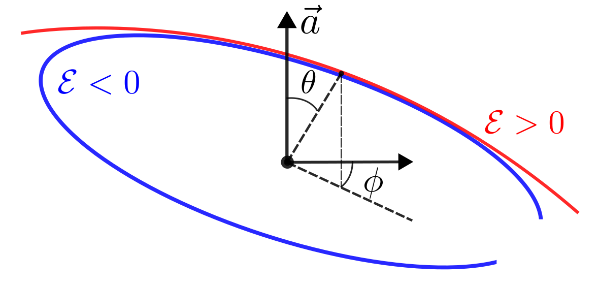
Figure 1: We consider a class of orbits in a Kerr black hole which smoothly interpolates between scattering ($\mathcal{E}>0$, in red) and bound ($\mathcal{E}<0$, in blue) dynamics.

Conventions

We use the mostly plus signature convention $(-+++)$ for the metric and we set $c=1$.

II Hamilton-Jacobi action for generic Kerr orbits

The Kerr metric describes the spacetime of a spinning black hole of mass $M$ and spin $J=Ma$. This can be written in Boyer-Lindquist coordinates $(t,r,\theta,\phi)$ as

$$\mathrm{d}s^{2} =-\frac{\Delta}{\Sigma}(\mathrm{d}t-a\sin^{2}(\theta)\mathrm{d}\phi)^{2}+\frac{\Sigma}{\Delta}\mathrm{d}r^{2}+\Sigma\,\mathrm{d}\theta^{2}$$ (1)

$$\quad+\frac{\sin^{2}(\theta)}{\Sigma}[(r^{2}+a^{2})\mathrm{d}\phi-a\mathrm{d}t]^{2}\,,$$

$$\Delta(r) =r^{2}-2Mr+a^{2}\,,\quad\Sigma(r,\theta)=r^{2}+a^{2}\cos^{2}(\theta)\,,$$

where we have set Newton’s constant to unity $G=1$ and we have chosen the reference axis to be aligned with the spin direction. The relativistic Hamiltonian for the geodesic motion of a probe particle of mass $m$ and 4-momentum $p_{\mu}$ in this metric is $H(x,p)=1/2\,g^{\mu\nu}p_{\mu}p_{\nu}$, which guarantees the validity of the geodesic equations

$$p^{\mu}\nabla_{\mu}p^{\nu}=0\,,\qquad g^{\mu\nu}p_{\mu}p_{\nu}=-m^{2}\,.$$ (2)

A complete set of constants of motion can be determined for Kerr, as first shown by Carter [82]. First of all, the metric (1) admits two Killing vectors $\partial_{t}$ and $\partial_{\phi}$ as a consequence of time-translation and axial symmetry. Therefore, the total energy $E$ and the angular momentum parallel to the spin axis $L$ as seen by an observer at spatial infinity are conserved

$$E:=-p_{\mu}\partial^{\mu}_{t}=-p_{t}\,,\qquad L:=p_{\mu}\partial^{\mu}_{\phi}=p_{\phi}\,.$$ (3)

In addition to the isometries, the Kerr metric admits also an irreducible symmetric Killing tensor $K_{\mu\nu}$ which implies the existence of a new conserved charge $Q$ called the Carter integral

$$Q =K^{\mu\nu}p_{\mu}p_{\nu}-(L-aE)^{2}$$ (4)

$$=p_{\theta}^{2}+a^{2}(m^{2}-p_{t}^{2})\cos^{2}(\theta)+p_{\phi}^{2}\cot^{2}(\theta)\,.$$

Using a Euclidean flat space 3$d$ notation [86, 87], we can write $\vec{r}=r(\sin(\theta)\cos(\phi),\sin(\theta)\sin(\phi),\cos(\theta))$ and $\vec{a}=(0,0,a)$ so that we can suggestively recast (4) as

$$Q =|\vec{r}\wedge\vec{p}|^{2}-(\vec{r}\wedge\vec{p}\cdot\hat{a})^{2}-|\vec{p}|^{2}(a\cdot\hat{r})^{2}$$ (5)

$$=|\vec{L}|^{2}-L^{2}-|\vec{p}|^{2}(a\cdot\hat{r})^{2}\,,$$

i.e. this is a measure of the motion of the particle off the equatorial plane given by the generalization of the equatorial projection of the orbital angular momentum $|\vec{L}|^{2}-L^{2}$ for a spinning source [88]. For the scattering case, the relation between the conserved charges and the incoming kinematics is summarized in appendix A.

The instantaneous 4-momentum $\mathcal{P}=p_{\mu}\mathrm{d}x^{\mu}$ of the probe particle can be now expressed [90] in terms of the four constants of motion $(m^{2},E,L,Q)$ by directly inverting the equations (2),(3) and (4)

$$\mathcal{P}(x):=-E\,\mathrm{d}t\pm_{r}\frac{\sqrt{R(r)}}{\Delta(r)}\,\mathrm{d}r\pm_{\theta}\sqrt{\Theta(\theta)}\,\mathrm{d}\theta+L\,\mathrm{d}\phi\,,$$ (6)

where we have defined the polar and radial potential

$$\Theta(\theta) :=Q+a^{2}(E^{2}-m^{2})\cos^{2}(\theta)-L^{2}\cot^{2}(\theta)\,,$$ (7)

$$R(r) :=[E(r^{2}+a^{2})-aL]^{2}-\Delta(Q+(L-aE)^{2}+m^{2}r^{2})\,,$$

the signs $\pm_{r}$ and $\pm_{\theta}$ depend on the radial and polar direction of the motion, respectively. For convenience, we choose $\pm_{r}=\pm_{\theta}=+$. The canonical 1-form (6) provides the transformation to the principal function $S$, in terms of which the HJ action $I$ is defined as

$$\qquad\quad I:=S+Et-L\phi=I_{r}+I_{\theta}\,,$$ (8)

$$I_{r} =\frac{1}{2\pi}\int_{\mathcal{C}_{r}}p_{r}\,\mathrm{d}r\,,\qquad\,\,\,\,\,\,\,\,\,\,\,I_{\theta}=\frac{1}{2\pi}\int_{\mathcal{C}_{\theta}}p_{\theta}\,\mathrm{d}\theta\,,$$

where the paths $\mathcal{C}_{r}$ and $\mathcal{C}_{\theta}$ correspond to the physical trajectories for the radial and polar motion. Since the dynamics in a Kerr spacetime is separable in Boyer-Lindquist coordinates, those contours $\mathcal{C}_{k}$ can be localized within the $(x^{k},p_{k})$ plane on the cotangent bundle.

II.1 Boundary to bound dictionary for generic orbits

We are interested in a class of generic orbits that smoothly connects the scattering and the bound regime. Generic geodesics are such that both endpoints are either a simple root of the radial potential $R(r)$, the horizon or infinity. The classification of time-like and null-like orbits in terms of the radial root structure has been recently completed in [91] and [92], respectively. We employ the conventions introduced in [91] for the radial roots, which we review here. We use the symbols $\mid,+,-$ and $\rangle$ to label respectively the Kerr outer horizon, a region where motion is allowed $(R>0)$, a region where motion is disallowed $(R<0)$ and radial infinity, and the $\bullet$ to denote a single root. The radial root structure of the class of geodesics we are interested in is discussed in table 1.

Type	Energy range	Root structure	Radial range
Unbound	$E>m$	$|+\bullet-{\color[rgb]{1,0,0}\bullet}+\rangle$	$r_{m}\leq r<\infty$
Bound	$E_{\text{ISCO}^{+}}<E<m$	$|+\bullet-{\color[rgb]{1,0,0}\bullet}+{\color[rgb]{0,0,1}\bullet}-\rangle$	$r_{-}\leq r\leq r_{+}$

Table 1: The table shows the specific class of unbound orbits ($E>m$) with a single turning point $r_{m}$ (in red) that are smoothly connected with bound orbits ($E<m$) with two turning points $r_{-}$ (in red), $r_{+}$ (in blue).

At this point, we can define the cycle of integration for the Hamilton-Jacobi action for unbound and bound geodesics. We introduce the superscript $>$ to denote an expression valid for scattering orbits and $<$ to denote an expression valid for bound ones. For the radial motion, making manifest the dependence of the radial roots on the conserved charges, the radial integral becomes

$$\int_{\mathcal{C}_{r}^{>}}=2\int_{r_{m}(\mathcal{E},l,a,l_{Q})}^{\infty}\,,\qquad\int_{\mathcal{C}_{r}^{<}}=2\int_{r_{-}(\mathcal{E},l,a,l_{Q})}^{r_{+}(\mathcal{E},l,a,l_{Q})}\,,$$ (9)

where we have defined the conserved quantities per unit mass,

$$\mathcal{E}:=\frac{E^{2}-m^{2}}{m^{2}}\,,\quad l:=\frac{L}{m}\,,\quad l_{Q}:=\frac{\sqrt{Q+L^{2}}}{m}$$ (10)

A direct inspection of the analytic structure of the radial roots shows that we can generalize the boundary to bound dictionary from equatorial orbits [72, 73] to generic orbits because of the remarkable map

$$r_{-}(\mathcal{E},l,a,l_{Q}) \stackrel{{\scriptstyle\mathcal{E}<0}}{{=}}r_{m}(\mathcal{E},l,a,l_{Q})\,,$$ (11)

$$r_{+}(\mathcal{E},l,a,l_{Q}) \stackrel{{\scriptstyle\mathcal{E}<0}}{{=}}r_{m}(\mathcal{E},-l,-a,-l_{Q})\,,$$

where $l_{Q}$ plays the role of an angular momentum.

For the polar motion, the condition $\Theta\geq 0$ implies that a generic geodesic with $l\neq 0$ is bounded between two turning points $\theta_{-}<\theta<\theta_{+}$, which are the solutions of the equation $\Theta=0$ . The polar motion can be of ordinary or of vortical type according to the value of $\theta_{\pm}$, as shown in table 2.

Type	Polar range	Conditions
Ordinary	$\theta_{-}<\pi/2<\theta_{+}$, $\theta_{-}=\pi-\theta_{+}$	$Q>0,\mathcal{E}\lessgtr 0$
Vortical	$\theta_{-}<\theta_{+}<\pi/2$ or $\pi/2<\theta_{-}<\theta_{+}$	$Q\leq 0,\mathcal{E}>0$

Table 2: The table provides a qualitative classification of the polar motion.

Since we are interested in a class of geodesics that connect the unbound ($\mathcal{E}>0$) and the bound ($\mathcal{E}<0$) regime, we are forced to restrict to the case of the oscillatory polar motion with $Q>0$. After excluding the degenerate case of planar geodesics at fixed polar angle $\theta=\theta_{\pm}$, the angular integral for the generic configuration reads [90]

$$\int_{\mathcal{C}_{\theta}}=2n\Bigg{|}\int_{\pi/2}^{\theta_{\pm}}\Bigg{|}+\eta_{\text{in}}\Bigg{|}\int_{\pi/2}^{\theta_{\text{in}}}\Bigg{|}-\eta_{\text{out}}\Bigg{|}\int_{\pi/2}^{\theta_{\text{out}}}\Bigg{|}\,,$$ (12)

where $\theta_{\text{in}}$ (resp. $\theta_{\text{out}}$) is the initial (resp. final) polar angle of the trajectory, $n$ is the number of turning points of the polar motion and we have defined the signs

$$\eta_{\text{in}/\text{out}} =\text{sign}(p_{\text{in}/\text{out}}^{\theta})\,\text{sign}(\cos(\theta_{\text{in}/\text{out}}))\,.$$ (13)

We now consider the class of geodesics which start on the equatorial plane with $\theta_{\text{in}}=\pi/2$, which is a convenient simplification of our problem and will not affect the validity of the analytic continuation. With this choice, the physical observables we will compute depend only on the conserved charges. Therefore, we can effectively use

$$\int_{\mathcal{C}_{\theta}}\to 2n\Bigg{|}\int_{\pi/2}^{\theta_{\pm}}\Bigg{|}-\eta_{\text{out}}\Bigg{|}\int_{\pi/2}^{\theta_{\text{out}}}\Bigg{|}\,,$$ (14)

where $\theta_{\text{out}}$ will be determined explicitly in terms of the conserved charges, as we will discuss later.

We are now ready to compute the Hamilton-Jacobi action for our class of geodesics. We start with the radial action, which we can write for scattering orbits as

$$I_{r}^{>} :=\frac{1}{2\pi}\int_{\mathcal{C}_{r}^{>}}p_{r}\,\mathrm{d}r\stackrel{{\scriptstyle u=1/r}}{{=}}\frac{1}{\pi}\int_{0}^{u_{m}}\frac{\mathrm{d}u}{u^{2}}\frac{\sqrt{R(u)}}{\Delta(u)}$$ (15)

$$=\frac{1}{2\pi}\frac{\sqrt{\mathcal{E}}}{\sqrt{M^{2}-a^{2}}}$$

$$\,\,\times\int_{0}^{u_{m}}\frac{\mathrm{d}u}{u^{2}}\prod_{j=1}^{4}\left(1-\frac{u}{u_{j}}\right)^{\frac{1}{2}}\left(\frac{1}{u_{B}-u}-\frac{1}{u_{A}-u}\right)\,,$$

where we have defined the radial roots $\{u_{j}\}_{j=1,\dots,4}$ and

$$R(u)=- \frac{a^{2}Q}{u^{4}}\prod_{j=1}^{4}(u-u_{j})\,,$$ (16)

$$u_{A}=\frac{M+\sqrt{M^{2}-a^{2}}}{a^{2}}\,, \,\,\,u_{B}=\frac{M-\sqrt{M^{2}-a^{2}}}{a^{2}}\,.$$

Having selected the radial root corresponding to the minimum distance according to the pattern identified in table 1, say $u_{4}=u_{m}$, we can then change variables to $u=u_{m}\tilde{u}$ so that the radial action reads

$$I_{r}^{>,\epsilon} =\frac{1}{2\pi}\frac{m\sqrt{\mathcal{E}}}{u_{m}^{1-\epsilon}\sqrt{M^{2}-a^{2}}}\int_{0}^{1}\frac{\mathrm{d}\tilde{u}}{\tilde{u}^{2-\epsilon}}$$ (17)

$$\times\prod_{j=1}^{4}\left(1-\frac{u_{m}}{u_{j}}\tilde{u}\right)^{\frac{1}{2}}\left[\frac{1}{u_{B}-u_{m}\tilde{u}}-\frac{1}{u_{A}-u_{m}\tilde{u}}\right]\,,$$

where we have introduced an infrared regulator $\epsilon>0$ to make the integral well-defined [64, 4]. We can then provide a closed-form expression for the radial action in terms of the Lauricella hypergeometric functions $F_{D}^{(n)}$,

$$I_{r}^{>,\epsilon}=\frac{1}{2\pi}\frac{m\sqrt{\mathcal{E}}}{u_{m}^{1-\epsilon}\sqrt{M^{2}-a^{2}}}\frac{\Gamma(-1+\epsilon)\Gamma(3/2)}{\Gamma(1/2+\epsilon)}$$ (18)

$$\times\!\bigg{[}\frac{1}{u_{B}}F_{D}^{(4)}\bigg{(}\alpha_{r},\vec{\beta}_{r},\gamma_{r};\frac{u_{m}}{u_{B}},\frac{u_{m}}{u_{1}},\frac{u_{m}}{u_{2}},\frac{u_{m}}{u_{3}}\bigg{)}\!-\!(u_{B}\!\leftrightarrow\!u_{A})\bigg{]}$$

$$\alpha_{r}=-1+\epsilon,\quad\vec{\beta}_{r}=\Big{\{}1,-\frac{1}{2},-\frac{1}{2},-\frac{1}{2}\Big{\}},\quad\gamma_{r}=\frac{1}{2}+\epsilon\,.$$

For bound orbits, we can use the relation (11) to write the radial contour as

$$\int_{\mathcal{C}_{r}^{<}} \stackrel{{\scriptstyle\mathcal{E}<0}}{{=}}\int_{r_{-}(\mathcal{E},l,a,l_{Q})}^{\infty}-\int_{r_{+}(\mathcal{E},l,a,l_{Q})}^{\infty}$$ (19)

$$\stackrel{{\scriptstyle\mathcal{E}<0}}{{=}}\int_{r_{m}(\mathcal{E},l,a,l_{Q})}^{\infty}-\int_{r_{m}(\mathcal{E},-l,-a,-l_{Q})}^{\infty}\,.$$

Since $p_{r}$ is invariant under $(a,l,l_{Q})\to(-a,-l,-l_{Q})$, we can establish the analytic continuation

$$I_{r}^{<,\epsilon}(\mathcal{E},l,a,l_{Q})$$ (20)

$$\quad\stackrel{{\scriptstyle\mathcal{E}<0}}{{=}}I_{r}^{>,\epsilon}(\mathcal{E},l,a,l_{Q})-I_{r}^{>,\epsilon}(\mathcal{E},-l,-a,-l_{Q})\,.$$

At this point, we focus on the polar action and we compute separately the contribution of both terms in (14). Once we choose the initial condition $\text{sign}(p_{\text{in}}^{\theta})=1$, the equations of motion will impose (see appendix B)

$$\eta^{>}_{\text{out}}=-1\,,\quad n^{>}=1\,,\qquad\eta^{<}_{\text{out}}=+1\,,\quad n^{<}=2\,,$$ (21)

for scattering and bound orbits, respectively. The first contribution for scattering orbits reads

$$I_{\theta}^{>(1)} :=\frac{1}{2\pi}\int_{\mathcal{C}_{\theta}^{>}}p_{\theta}\,\mathrm{d}\theta\Bigg{|}_{1}=\frac{n^{>}}{\pi}\int_{\pi/2}^{\theta_{+}}\mathrm{d}\theta\,\sqrt{\Theta(\theta)}$$ (22)

$$\!\!\!\!\!\!\!\stackrel{{\scriptstyle\cos^{2}(\theta)=U_{+}\tilde{U}}}{{=}}\frac{\sqrt{QU_{+}}}{2\pi}\int_{0}^{1}\frac{\mathrm{d}\tilde{U}(1-\tilde{U})^{\frac{1}{2}}}{\tilde{U}^{\frac{1}{2}}(1-U_{+}\tilde{U})}\left(1-\frac{U_{+}}{U_{-}}\tilde{U}\right)^{\frac{1}{2}}\,,$$

where the roots $U_{\pm}$ of the polar potential are

$$U_{\pm}\! =\!\frac{\Delta U\!\pm\!\sqrt{\Delta U^{2}\!+\!a^{2}\mathcal{E}(l_{Q}^{2}-l^{2})}}{a^{2}\mathcal{E}}\,,$$ (23)

$$\qquad\Delta U=\frac{a^{2}\mathcal{E}-l_{Q}^{2}}{2}\,,$$

and it is possible to show that $\theta_{\mp}=\arccos(\pm\sqrt{U_{+}})$. Therefore, the first term can be written in terms of the Lauricella hypergeometric function $F_{D}^{(q)}$,

$$I_{\theta}^{>(1)} =\frac{1}{4}\sqrt{QU_{+}}F_{D}^{(2)}\left(\alpha^{(1)}_{\theta},\vec{\beta}^{(1)}_{\theta},\gamma^{(1)}_{\theta};U_{+},\frac{U_{+}}{U_{-}}\right)\,,$$ (24)

$$\alpha^{(1)}_{\theta}=\frac{1}{2},\quad\vec{\beta}^{(1)}_{\theta}=\Big{\{}1,-\frac{1}{2}\Big{\}},\quad\gamma^{(1)}_{\theta}=2\,.$$

Therefore the second term in (14) can be written as

$$I_{\theta}^{>(2)}=\frac{1}{2\pi}\int_{\mathcal{C}_{\theta}^{>}}p_{\theta}\,\mathrm{d}\theta\Bigg{|}_{2}=-\frac{\eta_{\text{out}}^{>}}{2\pi}\int_{\pi/2}^{\theta_{\text{out}}^{>}}\mathrm{d}\theta\,\sqrt{\Theta(\theta)}$$ (25)

$$=\frac{1}{2\pi}\sqrt{QU^{>}_{\text{out}}}F_{D}^{(3)}\left(\alpha^{(2)}_{\theta},\vec{\beta}^{(2)}_{\theta},\gamma^{(2)}_{\theta};U^{>}_{\text{out}},\frac{U^{>}_{\text{out}}}{U_{+}},\frac{U^{>}_{\text{out}}}{U_{-}}\right)\,,$$

$$\qquad\alpha^{(2)}_{\theta}=\frac{1}{2},\quad\vec{\beta}^{(2)}_{\theta}=\Big{\{}1,-\frac{1}{2},-\frac{1}{2}\Big{\}},\quad\gamma^{(2)}_{\theta}=\frac{3}{2}\,,$$

where the $U^{>}_{\text{out}}$ is determined from (see [90])

$$U^{>}_{\text{out}} =U_{+}\operatorname{sn}^{2}\left(X_{0}^{>}\Big{|}\frac{U_{-}}{U_{+}}\right)\,,$$ (26)

$$X_{0}^{>} =-\sqrt{-a^{2}m^{2}\mathcal{E}U_{-}}\int_{\mathcal{C}_{r}^{>}}\frac{\mathrm{d}r}{\sqrt{\mathcal{R}(r)}}\,.$$

For bound orbits, the turning points of the polar potential are still $\theta_{\mp}=\arccos(\pm\sqrt{U_{+}})$, so we only need to perform the conventional analytical continuation of the radial contour $\mathcal{C}_{r}^{>}\to\mathcal{C}_{r}^{<}$ for $U_{\text{out}}$ in (26). The polar action for $\mathcal{E}<0$ will therefore be

$$I^{<}_{\theta}(\mathcal{E},l,a,l_{Q}; n^{>},\eta_{\text{out}}^{>})\stackrel{{\scriptstyle\mathcal{E}<0}}{{=}}I^{>}_{\theta}(\mathcal{E},l,a,l_{Q};n^{<},\eta_{\text{out}}^{<})\,,$$ (27)

where we emphasize again that $n^{>}=1\to n^{<}=2$ and $\eta^{>}_{\text{out}}=-1\to\eta^{<}_{\text{out}}=+1$ as a consequence of the analytic continuation of the equations of motion.

III Perturbative expansion of scattering observables

In this section we derive the post-Minkowskian (PM) expansion of the scattering angles $(\Delta\theta,\Delta\phi)$ and the time delay $\Delta T$ by using the equations of motion coming from the HJ action (8). Since our main focus is on the weak field limit, we present our results as a double expansion in $M$ and $a$ with $a\ll M$. We refer the reader to appendix C for the exact expression of scattering angles in terms of hypergeometric functions.

III.1 Polar deflection angle $\Delta\theta$

The polar deflection angle $\Delta\theta=\theta_{\text{out}}-(\pi-\theta_{\text{in}})$ is completely determined by $U_{\text{out}}=\cos^{2}(\theta_{\text{out}})$, given that we set $\theta_{\text{in}}=\pi/2$. It is straightforward to extend all our calculations to a generic incoming angle $\theta_{\text{in}}$, for example by using the generic polar contour (12) in the $r-\theta$ equation (43) of appendix B. A direct perturbative expansion of $\Delta\theta$ from (26) gives, up to $\mathcal{O}(M^{3}a^{2})$,

$$\frac{\Delta\theta}{\sqrt{l_{Q}^{2}-l^{2}}}=-\frac{2M(2\mathcal{E}+1)}{\sqrt{\mathcal{E}}\,l_{Q}^{2}}-\frac{3\pi M^{2}(5\mathcal{E}+4)}{4\,l_{Q}^{3}}$$ (28)

$$\qquad-\frac{2M^{3}(64\mathcal{E}^{3}+72\mathcal{E}^{2}+12\mathcal{E}\!-\!1)}{3\,\mathcal{E}^{3/2}\,l_{Q}^{4}}+\frac{4M^{3}l^{2}(2\mathcal{E}+1)^{3}}{3\,\mathcal{E}^{3/2}\,l_{Q}^{6}}$$

$$\qquad+a\sqrt{\mathcal{E}+1}\Bigg{(}\frac{8Ml\sqrt{\mathcal{E}}}{l_{Q}^{4}}+\frac{3\pi M^{2}l(5\mathcal{E}+2)}{l_{Q}^{5}}$$

$$\qquad-\frac{16M^{3}l^{3}(2\mathcal{E}+1)^{2}}{\sqrt{\mathcal{E}}\,l_{Q}^{8}}+\frac{16M^{3}l(16\mathcal{E}^{2}+12\mathcal{E}+1)}{\sqrt{\mathcal{E}}\,l_{Q}^{6}}\Bigg{)}$$

$$+a^{2}\Bigg{(}\frac{2\sqrt{\mathcal{E}}M(l_{Q}^{2}-4\,l^{2})(2\mathcal{E}+1)}{l_{Q}^{6}}$$

$$\qquad+\frac{3\pi M^{2}(l_{Q}^{2}-5\,l^{2})(95\mathcal{E}^{2}+88\mathcal{E}+8)}{32\,l_{Q}^{7}}$$

$$\qquad+\frac{16M^{3}l^{4}(2\mathcal{E}+1)(8\mathcal{E}^{2}+8\mathcal{E}+1)}{\sqrt{\mathcal{E}}\,l_{Q}^{10}}$$

$$\qquad-\frac{12M^{3}l^{2}(88\mathcal{E}^{3}+116\mathcal{E}^{2}+34\mathcal{E}+1)}{\sqrt{\mathcal{E}}\,l_{Q}^{8}}$$

$$\qquad+\frac{8M^{3}\sqrt{\mathcal{E}}(20\mathcal{E}^{2}+26\mathcal{E}+7)}{l_{Q}^{6}}\Bigg{)}\,.$$

III.2 Azimuthal deflection angle $\Delta\phi$

The azimuthal scattering angle $\Delta\phi$ is the conjugate variable to the angular momentum $L$, i.e.

$$\frac{\Delta\phi+\pi}{2\pi}=-\frac{\partial I}{\partial L}=-\frac{\partial I_{r}}{\partial L}-\frac{\partial I_{\theta}}{\partial L}\,,$$ (29)

which can be computed from the Hamilton-Jacobi action in (18), (22) and (24). It is worth stressing that we need to keep $U^{>}_{\text{out}}$ invariant in taking the derivative over $L$, since technically it is only fixed dynamically by the equations of motion, whereas the HJ action works at the off-shell level . A direct calculation up to order $\mathcal{O}(M^{3}a^{2})$ in the PM expansion gives

$$\Delta\phi=\frac{2Ml(2\mathcal{E}+1)}{\sqrt{\mathcal{E}}\,l_{Q}^{2}}+\frac{3\pi M^{2}l(5\mathcal{E}+4)}{4\,l_{Q}^{3}}$$ (30)

$$\qquad+\frac{2M^{3}l(64\mathcal{E}^{3}+72\mathcal{E}^{2}+12\mathcal{E}-1)}{3\,\mathcal{E}^{3/2}\,l_{Q}^{4}}$$

$$+a\sqrt{\mathcal{E}+1}\Bigg{(}\frac{4M\sqrt{\mathcal{E}}(l_{Q}^{2}-2l^{2})}{l_{Q}^{4}}$$

$$\qquad+\frac{\pi M^{2}(5\mathcal{E}+2)(l_{Q}^{2}-3l^{2})}{l_{Q}^{5}}$$

$$\qquad+\frac{4M^{3}(16\mathcal{E}^{2}+12\mathcal{E}+1)(l_{Q}^{2}-4l^{2})}{\sqrt{\mathcal{E}}\,l_{Q}^{6}}\Bigg{)}$$

$$+a^{2}\Bigg{(}\frac{2M\sqrt{\mathcal{E}}(2\mathcal{E}+1)(4l^{2}-3l_{Q}^{2})}{l_{Q}^{6}}$$

$$\qquad+\frac{3\pi M^{2}l(95\mathcal{E}^{2}+88\mathcal{E}+8)(5l^{2}-3l_{Q}^{2})}{32\,l_{Q}^{7}}$$

$$\qquad+\frac{4M^{3}l(128\mathcal{E}^{3}+168\mathcal{E}^{2}+48\mathcal{E}+1)(2l^{2}-l_{Q}^{2})}{\sqrt{\mathcal{E}}\,l_{Q}^{8}}\Bigg{)}$$

$$+M^{3}(l_{Q}^{2}-l^{2})\Bigg{[}\frac{8l(2\mathcal{E}+1)^{3}}{3\,\mathcal{E}^{3/2}\,l_{Q}^{6}}-\frac{32a\,l^{2}\sqrt{\mathcal{E}+1}(2\mathcal{E}+1)^{2}}{\sqrt{\mathcal{E}}\,l_{Q}^{8}}$$

$$\quad+\frac{8a^{2}l(2\mathcal{E}+1)\left(4l^{2}\left(8\mathcal{E}^{2}+8\mathcal{E}+1\right)-(2\mathcal{E}+1)^{2}l_{Q}^{2}\right)}{\sqrt{\mathcal{E}}\,l_{Q}^{10}}\Bigg{]}\,,$$

where we have isolated with the last square bracket the contributions from the polar action, which are proportional to $Q=m^{2}(l_{Q}^{2}-l^{2})$. It is possible to notice a simple relation between the angles $\Delta\phi$ and $\Delta\theta$ as $a\to 0$, i.e. $\Delta\phi\stackrel{{\scriptstyle a\to 0}}{{\sim}}-(l/\sqrt{l_{Q}^{2}-l^{2}})\Delta\theta$ at the lowest order, which is determined by the fact that the motion happens on an inclined plane and there is always a change of coordinates to bring it to the standard equatorial plane. Moreover, in the limit $l_{Q}\to l$, we recover as expected the well-known equatorial expression [32, 98].

III.3 Time delay

The time delay is related to the conjugate variable of the energy $E$ in the HJ action, but it is defined only when we compare the measure to an observer at large distances [99, 100, 56, 101]. Having defined the impact parameter $b$ for generic null geodesics

$$r_{m}\stackrel{{\scriptstyle M\to 0}}{{=}}b=|\vec{b}|\longrightarrow b=\frac{\sqrt{L^{2}+Q}}{E}\,,$$ (31)

and the effective inclination angle [102]

$$\cos(\iota)=\frac{L}{\sqrt{L^{2}+Q}}\,,$$ (32)

we can then compute the time delay $\Delta T$ for generic null geodesics with fixed $b$ relative to an observer with $b^{\prime}\gg b$ but at the same energy $E^{\prime}=E$,

$$\Delta T =\frac{\partial I}{\partial E}\Bigg{|}_{b,E}-\frac{\partial I}{\partial E}\Bigg{|}_{b^{\prime}\gg b,E^{\prime}=E}$$ (33)

$$=4M\log\left(\frac{b^{\prime}}{b}\right)+\frac{15\pi M^{2}}{2\,b}+\frac{64M^{3}}{b^{2}}$$

$$-\frac{a\cos(\iota)}{b}\left(8M+\frac{15\pi M^{2}}{b}+\frac{256M^{3}}{b^{2}}\right)$$

$$+\frac{a^{2}}{b^{2}}\Big{(}6M\cos(2\iota)+\frac{95\pi M^{2}}{16\,b}(1+3\cos(2\iota))$$

$$\qquad\qquad\qquad+\frac{32M^{3}}{b^{2}}(7+13\cos(2\iota))\Big{)}\,,$$

which is accurate up to order $\mathcal{O}(M^{3}a^{2})$. As expected, $\Delta T$ is positive because of causality arguments [99] as long as we impose the physical condition $a\leq M$.

IV Perturbative expansion of bound observables

Using the boundary to bound dictionary for the Hamilton-Jacobi action developed in (20) and (27), we now proceed to compute the perturbative expansion of bound observables for generic bound orbits which are connected to scattering ones via analytic continuation. We use the same conventions as in section III.

IV.1 The fundamental frequencies $\omega_{r},\omega_{\phi},\omega_{\theta}$

The basic properties of Kerr bound orbits are specified by the so-called fundamental frequencies [83, 103, 104]. Although they are coordinate independent, it is useful to describe them via the conjugate momenta of the action-angle variables in the Boyer-Lindquist representation,

$$J_{t}:=E,\qquad J_{r}:=\frac{1}{2\pi}\oint p_{r}\,\mathrm{d}r=I_{r}^{<},$$ (34)

$$J_{\theta}:=\frac{1}{2\pi}\oint p_{\theta}\mathrm{d}\theta=I_{\theta}^{<(1)},\quad J_{\phi}:=\frac{1}{2\pi}\oint p_{\phi}\mathrm{d}\phi=L.$$

Since the coordinates are integrated out, the action momenta are constants of the motion $J_{\beta}(H,E,L,Q)$, where $H=-m^{2}/2$ is the Hamiltonian for the action-angle variables. The fundamental frequencies are defined as

$$\omega_{r}=\frac{\partial H}{\partial J_{r}}\,,\quad\omega_{\theta}=\frac{\partial H}{\partial J_{\theta}}\,,\quad\omega_{\phi}=\frac{\partial H}{\partial J_{\phi}}\,.$$ (35)

Note that the partial derivative are taken with $J_{\beta}$ being invariant. Using the results in appendix D, we can express these frequencies as

$$\omega_{r}=-\frac{1}{\Omega}\frac{\partial J_{\theta}}{\partial Q}\,,\quad\omega_{\theta}=\frac{1}{\Omega}\frac{\partial J_{r}}{\partial Q}\,,$$ (36)

$$\omega_{\phi}=\frac{1}{\Omega}\bigg{(}\frac{\partial J_{r}}{\partial L}\frac{\partial J_{\theta}}{\partial Q}-\frac{\partial J_{r}}{\partial Q}\frac{\partial J_{\theta}}{\partial L}\bigg{)}\,,$$

with $\Omega:=\frac{\partial J_{r}}{\partial H}\frac{\partial J_{\theta}}{\partial Q}-\frac{\partial J_{r}}{\partial Q}\frac{\partial J_{\theta}}{\partial H}$. These frequencies have been computed in a closed form in [83, 84], but they do not generically admit a weak field expansion. Indeed, these are considered only as “infinite time average” bound observables because of dependence on the choice of the time parametrization for each coordinate. Therefore the natural bound observables are the frequency ratios [105]

$$K^{\phi r}:=\frac{\omega_{\phi}}{\omega_{r}}=\frac{\partial J_{r}/\partial Q}{\partial J_{\theta}/\partial Q}\,\frac{\partial J_{\theta}}{\partial L}-\frac{\partial J_{r}}{\partial L},$$ (37)

$$K^{\theta r}:=\frac{\omega_{\theta}}{\omega_{r}}=-\frac{\partial J_{r}/\partial Q}{\partial J_{\theta}/\partial Q}\,,$$ (38)

which are related to the precession rate of the periastron ($K^{\phi r}$) and of the orbital plane ($K^{\theta r}$).

IV.2 The periastron precession rate $\omega_{\phi}/\omega_{r}$

In the weak field regime, we can identify the precession rate of the orbital ellipse with the so-called periastron advance rate $K^{\phi r}$. A direct calculation of (37) gives, up to order $\mathcal{O}(M^{3}a^{2})$ in the weak-field expansion,

$$K^{\phi r} =1+\frac{3M^{2}(5\mathcal{E}+4)}{4\,l_{Q}^{2}}$$ (39)

$$\quad+\frac{a\,M^{2}\sqrt{\mathcal{E}+1}(l_{Q}-3l)(5\mathcal{E}+2)}{l_{Q}^{4}}$$

$$\quad+\frac{3a^{2}M^{2}}{32\,l_{Q}^{6}}\Big{[}l^{2}(445\mathcal{E}^{2}+416\mathcal{E}+40)$$

$$\qquad\qquad\qquad-l_{Q}(l_{Q}+2l)(85\mathcal{E}^{2}+80\mathcal{E}+8)\Big{]}\,.$$

In the equatorial limit $l_{Q}\to l$ we find perfect agreement with the expression in the literature [73, 72].

IV.3 The orbital plane precession rate $\omega_{\theta}/\omega_{r}$

The orbital plane precession rate $K^{\theta r}$ can be essentially identified, in the weak field limit, with the Lense-Thirring effect. Using (38), we obtain up to $\mathcal{O}(M^{3}a^{2})$

$$K^{\theta r}=1+\frac{3M^{2}(5\mathcal{E}+4)}{4\,l_{Q}^{2}}-\frac{3aM^{2}l\sqrt{\mathcal{E}+1}(5\mathcal{E}+2)}{l_{Q}^{4}}$$ (40)

$$\qquad+\frac{3a^{2}M^{2}}{32\,l_{Q}^{6}}\Big{[}l^{2}(445\mathcal{E}^{2}+416\mathcal{E}+40)$$

$$\qquad\qquad\qquad\qquad\qquad-l_{Q}^{2}(85\mathcal{E}^{2}+80\mathcal{E}+8)\Big{]}\,.$$

In the limit $a\to 0$ the azimuthal and polar frequencies in (39)–(40) become degenerate $\omega_{\theta}=\omega_{\phi}$, while in the equatorial limit the polar one has no physical interpretation.

V Conclusion

In this paper, we have explored the relationship between scattering and bound observables for generic orbits in a Kerr background. The establishment of a boundary-to-bound dictionary represents a crucial step towards leveraging the computational tools that have been developed for scattering amplitudes in the study of bound systems. Expanding upon previous work in the field, we have extended such dictionary beyond the equatorial case by considering a smooth class of geodesics which interpolate between scattering and bound dynamics.

Taking advantage of the Hamilton-Jacobi representation, we have been able to write down a closed form expression for the radial and the polar contribution to the action for such generic class of scattering and bound orbits. In particular, we have found that in the PM expansion there is one turning point in the scattering case and two turning points in the bound case both for the radial and the polar motion. Such analytic continuation involves also the Carter constant, which plays a crucial role for the dynamics beyond the equatorial plane.

We have then computed, in the post-Minkowskian expansion, the azimuthal $\Delta\phi$ and the polar $\Delta\theta$ deflection angles for time-like geodesics in Kerr and the time delay $\Delta T$ for null geodesics. While the azimuthal angle is naturally derived from the action, the polar angle has a more implicit expression since there is no natural conjugate variable. Indeed in the conventional partial-wave basis an explicit relation has been found only for some degenerate configurations [106, 56], but perhaps an alternative basis might help to clarify the general case [58]. Using the new boundary to bound dictionary, we have then studied the weak-field expansion of the periastron and the orbital plane precession rate, $K^{\phi r}$ and $K^{\theta r}$, which are uniquely defined from the ratio of fundamental frequencies [83].

This work offers new promising directions for the analytic continuation of classical scattering and bound observables beyond the equatorial case. First, it would be important to extend the amplitude-action relation for generic angular momentum orientations, which would include some type of polar action contribution. Furthermore, a natural extension of our work would be to consider a spinning probe in a Kerr background [107], since a generalization of the Carter constant has been discovered by Rüdiger in the pole-dipole approximation [108, 109] and recently generalized to quadrupolar order [110]. Finally, it would be interesting to see how the extension of the Schwinger-Dyson recursion [81] would allow to compute radiative observables for bound orbits. We hope to come back to these questions in the near future.

Appendix A Conserved charges and kinematics

Here we present the relations between the conserved quantities and the kinematic invariants in the scattering case. Consider a probe particle with incoming momentum $p^{\mu}_{\text{in}}=(E,\vec{p}_{\text{in}})$ and impact parameter $b^{\mu}=(0,\vec{b})$, defined in such a way that $\vec{p}_{\text{in}}\cdot\vec{b}=0$. Then we have

$$E^{2}=|\vec{p}_{\text{in}}|^{2}+m^{2},$$

$$L^{2}=|\vec{p}_{\text{in}}|^{2}\big{(}|\vec{b}|^{2}-(\hat{a}\cdot\vec{b})^{2}\big{)}-|\vec{b}|^{2}(\hat{a}\cdot\vec{p}_{\text{in}})^{2},$$

$$Q=(|\vec{b}|^{2}-|\vec{a}|^{2})(\hat{a}\cdot\vec{p}_{\text{in}})^{2}+|\vec{p}_{\text{in}}|^{2}(\hat{a}\cdot\vec{b})^{2},$$ (41)

where $\hat{a}={\vec{a}}/{|\vec{a}|}$ is the unit vector along the spin direction. The incoming $\theta$ angle is determined by

$$U_{\mathrm{in}}=\cos^{2}(\theta_{\mathrm{in}})=(\hat{a}\cdot\hat{p}_{\text{in}})^{2}\,.$$ (42)

In the case considered in this letter $\theta_{\mathrm{in}}=\pi/2$ and therefore we have imposed $\hat{a}\cdot\hat{p}_{\text{in}}=0$.

Appendix B Turning points of the polar motion

The $(r,\theta)$ components of the geodesic equations in a Kerr black hole imply

$$\int_{\mathcal{C}_{r}}\frac{\mathrm{d}r}{\sqrt{R(r)}}=\int_{\mathcal{C}_{\theta}}\frac{\mathrm{d}\theta}{\sqrt{\Theta(\theta)}}\,,$$ (43)

from which we can find the final polar angle $U_{\text{out}}$, as discussed in section IID of [90]. A direct calculation for our setup shows that (43) can be reduced to

$$\sqrt{-a^{2}m^{2}\mathcal{E}U_{-}}\int_{\mathcal{C}_{r}^{>}}\frac{\mathrm{d}r}{\sqrt{R(r)}}$$ (44)

$$=2n^{>}K\left(\frac{U_{+}}{U_{-}}\right)-F\left(\arcsin\left(\sqrt{\frac{U_{\text{out}}^{>}}{U_{+}}}\right)\Big{|}\frac{U_{+}}{U_{-}}\right)$$

for the scattering case $\mathcal{E}>0$ and to

$$\sqrt{-a^{2}m^{2}\mathcal{E}U_{-}}\int_{\mathcal{C}_{r}^{<}}\frac{\mathrm{d}r}{\sqrt{R(r)}}$$ (45)

$$=2n^{<}K\left(\frac{U_{+}}{U_{-}}\right)+F\left(\arcsin\left(\sqrt{\frac{U_{\text{out}}^{<}}{U_{+}}}\right)\Big{|}\frac{U_{+}}{U_{-}}\right)$$

in the bound case $\mathcal{E}<0$. It is worth stressing that the sign flip reflects the fact that $\eta_{\text{out}}=-1$ for scattering orbits and $\eta_{\text{out}}=+1$ for the corresponding bound orbits. Since $U_{\text{out}}$ is independent of $n$, it turns that a perturbative expansion of (44) and (45) completely fix the number of turning points in the polar motion to

$$n^{>}=1\,,\qquad n^{<}=2\,.$$ (46)

Figure 2: A pictorial representation of the polar motion for the scattering (in red) and bound (in blue) class of geodesics of interest in this paper.

Appendix C Exact expressions for scattering observables

We provide here some compact resummed expressions for scattering observables in terms of hypergeometric functions (see also [111] for the equatorial case). These are always functions of the roots of the radial and polar potentials, which needs to be explicitly derived for the perturbative calculations.

The polar deflection angle is given by (26)

$$\qquad\cos^{2}(\theta_{\text{out}})=U_{+}\operatorname{sn}^{2}\left(X_{0}^{>}\Big{|}\frac{U_{-}}{U_{+}}\right)\,,\qquad\mathcal{E}>0\,,Q>0\,,$$

$$X_{0}^{>}=-4u_{m}\sqrt{-a^{2}U_{-}}\,F_{D}^{(3)}\left(\alpha_{\Delta\theta},\vec{\beta}_{\Delta\theta},\gamma_{\Delta\theta};\frac{u_{m}}{u_{1}},\frac{u_{m}}{u_{2}},\frac{u_{m}}{u_{3}}\right)\,,$$

$$\qquad\,\,\alpha_{\Delta\theta}=1,\quad\vec{\beta}_{\Delta\theta}=\Big{\{}\frac{1}{2},\frac{1}{2},\frac{1}{2}\Big{\}},\quad\gamma_{\Delta\theta}=\frac{3}{2}\,,$$ (47)

while the azimuthal deflection angle is derived from (29)

$$\Delta\phi=u_{m}\Bigg{[}\frac{G_{A}}{u_{A}}F_{D}^{(4)}\left(\alpha_{\Delta\phi_{1}},\vec{\beta}_{\Delta\phi_{1}},\gamma_{\Delta\phi_{1}};\frac{u_{m}}{u_{A}},\frac{u_{m}}{u_{1}},\frac{u_{m}}{u_{2}},\frac{u_{m}}{u_{3}}\right)$$

$$-\frac{G_{B}}{u_{B}}F_{D}^{(4)}\left(\alpha_{\Delta\phi_{1}},\vec{\beta}_{\Delta\phi_{1}},\gamma_{\Delta\phi_{1}};\frac{u_{m}}{u_{B}},\frac{u_{m}}{u_{1}},\frac{u_{m}}{u_{2}},\frac{u_{m}}{u_{3}}\right)\Bigg{]}$$

$$+\frac{\pi\,l\,U_{2}^{\frac{3}{2}}}{2\sqrt{l_{Q}^{2}-l^{2}}}F_{D}^{(2)}\left(\alpha_{\Delta\phi_{2}},\vec{\beta}_{\Delta\phi_{2}},\gamma_{\Delta\phi_{2}};U_{2},\frac{U_{2}}{U_{1}}\right)$$

$$+l\frac{(U^{>}_{\text{out}})^{\frac{3}{2}}}{3\sqrt{l_{Q}^{2}-l^{2}}}F_{D}^{(3)}\left(\alpha_{\Delta\phi_{3}},\vec{\beta}_{\Delta\phi_{3}},\gamma_{\Delta\phi_{3}};U^{>}_{\text{out}},\frac{U^{>}_{\text{out}}}{U_{1}},\frac{U^{>}_{\text{out}}}{U_{2}}\right)\,,$$

$$G_{A}=\frac{2Mu_{A}(l-a\mathcal{E})-l}{\sqrt{\mathcal{E}(M^{2}-a^{2})}}\,,G_{B}=\frac{2Mu_{B}(l-a\mathcal{E})-l}{\sqrt{\mathcal{E}(M^{2}-a^{2})}}\,,$$

$$\qquad\alpha_{\Delta\phi_{1}}=1,\quad\vec{\beta}_{\Delta\phi_{1}}=\Big{\{}1,\frac{1}{2},\frac{1}{2},\frac{1}{2}\Big{\}},\quad\gamma_{\Delta\phi_{1}}=\frac{3}{2}\,,$$

$$\qquad\alpha_{\Delta\phi_{2}}=\frac{3}{2},\quad\vec{\beta}_{\Delta\phi_{2}}=\Big{\{}1,\frac{1}{2}\Big{\}},\quad\gamma_{\Delta\phi_{2}}=2\,,$$

$$\qquad\alpha_{\Delta\phi_{3}}=\frac{3}{2},\quad\vec{\beta}_{\Delta\phi_{3}}=\Big{\{}1,\frac{1}{2},\frac{1}{2}\Big{\}},\quad\gamma_{\Delta\phi_{3}}=\frac{5}{2}\,.$$ (48)

Appendix D Derivation of the fundamental frequencies

The four integrals of motion

$$P_{\alpha}=\left(H,E,L,Q\right)=\left(-\frac{1}{2}m^{2},E,L,Q\right)\,,$$ (49)

are implicit functions of the action variables $P_{\alpha}=f(J_{\beta})$

$$J_{\beta}=(J_{t},J_{r},J_{\theta},J_{\phi})\,.$$ (50)

The fundamental frequencies can therefore be computed from the jacobian of $f$, i.e.

$$\frac{\partial P_{\alpha}}{\partial J_{\beta}}\frac{\partial J_{\beta}}{\partial P_{\gamma}}=\delta_{\alpha}^{\gamma}\,,$$ (51)

which gives directly (36).

References

- Abbott et al. [2016] B. P. Abbott et al. (LIGO Scientific, Virgo), Observation of Gravitational Waves from a Binary Black Hole Merger, Phys. Rev. Lett. 116, 061102 (2016), arXiv:1602.03837 [gr-qc] .
- Damour [2018] T. Damour, High-energy gravitational scattering and the general relativistic two-body problem, Phys. Rev. D 97, 044038 (2018), arXiv:1710.10599 [gr-qc] .
- Neill and Rothstein [2013] D. Neill and I. Z. Rothstein, Classical Space-Times from the S Matrix, Nucl. Phys. B 877, 177 (2013), arXiv:1304.7263 [hep-th] .
- Damour [2020] T. Damour, Classical and quantum scattering in post-Minkowskian gravity, Phys. Rev. D 102, 024060 (2020), arXiv:1912.02139 [gr-qc] .
- Bjerrum-Bohr et al. [2018] N. E. J. Bjerrum-Bohr, P. H. Damgaard, G. Festuccia, L. Planté, and P. Vanhove, General Relativity from Scattering Amplitudes, Phys. Rev. Lett. 121, 171601 (2018), arXiv:1806.04920 [hep-th] .
- Cheung et al. [2018] C. Cheung, I. Z. Rothstein, and M. P. Solon, From Scattering Amplitudes to Classical Potentials in the Post-Minkowskian Expansion, Phys. Rev. Lett. 121, 251101 (2018), arXiv:1808.02489 [hep-th] .
- Chung et al. [2019] M.-Z. Chung, Y.-T. Huang, J.-W. Kim, and S. Lee, The simplest massive S-matrix: from minimal coupling to Black Holes, JHEP 04, 156, arXiv:1812.08752 [hep-th] .
- Bern et al. [2019a] Z. Bern, C. Cheung, R. Roiban, C.-H. Shen, M. P. Solon, and M. Zeng, Black Hole Binary Dynamics from the Double Copy and Effective Theory, JHEP 10, 206, arXiv:1908.01493 [hep-th] .
- Bern et al. [2021a] Z. Bern, A. Luna, R. Roiban, C.-H. Shen, and M. Zeng, Spinning black hole binary dynamics, scattering amplitudes, and effective field theory, Phys. Rev. D 104, 065014 (2021a), arXiv:2005.03071 [hep-th] .
- Kosower et al. [2019] D. A. Kosower, B. Maybee, and D. O’Connell, Amplitudes, Observables, and Classical Scattering, JHEP 02, 137, arXiv:1811.10950 [hep-th] .
- Cristofoli et al. [2021] A. Cristofoli, R. Gonzo, N. Moynihan, D. O’Connell, A. Ross, M. Sergola, and C. D. White, The Uncertainty Principle and Classical Amplitudes, (2021), arXiv:2112.07556 [hep-th] .
- Maybee et al. [2019] B. Maybee, D. O’Connell, and J. Vines, Observables and amplitudes for spinning particles and black holes, JHEP 12, 156, arXiv:1906.09260 [hep-th] .
- Kälin and Porto [2020a] G. Kälin and R. A. Porto, Post-Minkowskian Effective Field Theory for Conservative Binary Dynamics, JHEP 11, 106, arXiv:2006.01184 [hep-th] .
- Mogull et al. [2021] G. Mogull, J. Plefka, and J. Steinhoff, Classical black hole scattering from a worldline quantum field theory, JHEP 02, 048, arXiv:2010.02865 [hep-th] .
- Bjerrum-Bohr et al. [2022a] N. E. J. Bjerrum-Bohr, P. H. Damgaard, L. Plante, and P. Vanhove, Chapter 13: Post-Minkowskian expansion from scattering amplitudes, J. Phys. A 55, 443014 (2022a), arXiv:2203.13024 [hep-th] .
- Vines [2018] J. Vines, Scattering of two spinning black holes in post-Minkowskian gravity, to all orders in spin, and effective-one-body mappings, Class. Quant. Grav. 35, 084002 (2018), arXiv:1709.06016 [gr-qc] .
- Guevara et al. [2019a] A. Guevara, A. Ochirov, and J. Vines, Scattering of Spinning Black Holes from Exponentiated Soft Factors, JHEP 09, 056, arXiv:1812.06895 [hep-th] .
- Guevara et al. [2019b] A. Guevara, A. Ochirov, and J. Vines, Black-hole scattering with general spin directions from minimal-coupling amplitudes, Phys. Rev. D 100, 104024 (2019b), arXiv:1906.10071 [hep-th] .
- Kosower et al. [2022] D. A. Kosower, R. Monteiro, and D. O’Connell, The SAGEX review on scattering amplitudes Chapter 14: Classical gravity from scattering amplitudes, J. Phys. A 55, 443015 (2022), arXiv:2203.13025 [hep-th] .
- Bern et al. [2019b] Z. Bern, C. Cheung, R. Roiban, C.-H. Shen, M. P. Solon, and M. Zeng, Scattering Amplitudes and the Conservative Hamiltonian for Binary Systems at Third Post-Minkowskian Order, Phys. Rev. Lett. 122, 201603 (2019b), arXiv:1901.04424 [hep-th] .
- Bern et al. [2022a] Z. Bern, J. Parra-Martinez, R. Roiban, M. S. Ruf, C.-H. Shen, M. P. Solon, and M. Zeng, Scattering Amplitudes, the Tail Effect, and Conservative Binary Dynamics at O(G4), Phys. Rev. Lett. 128, 161103 (2022a), arXiv:2112.10750 [hep-th] .
- Dlapa et al. [2022a] C. Dlapa, G. Kälin, Z. Liu, and R. A. Porto, Conservative Dynamics of Binary Systems at Fourth Post-Minkowskian Order in the Large-Eccentricity Expansion, Phys. Rev. Lett. 128, 161104 (2022a), arXiv:2112.11296 [hep-th] .
- Dlapa et al. [2022b] C. Dlapa, G. Kälin, Z. Liu, J. Neef, and R. A. Porto, Radiation Reaction and Gravitational Waves at Fourth Post-Minkowskian Order, (2022b), arXiv:2210.05541 [hep-th] .
- Di Vecchia et al. [2020] P. Di Vecchia, C. Heissenberg, R. Russo, and G. Veneziano, Universality of ultra-relativistic gravitational scattering, Phys. Lett. B 811, 135924 (2020), arXiv:2008.12743 [hep-th] .
- Di Vecchia et al. [2021] P. Di Vecchia, C. Heissenberg, R. Russo, and G. Veneziano, The eikonal approach to gravitational scattering and radiation at (G3), JHEP 07, 169, arXiv:2104.03256 [hep-th] .
- Bjerrum-Bohr et al. [2021] N. E. J. Bjerrum-Bohr, P. H. Damgaard, L. Planté, and P. Vanhove, The amplitude for classical gravitational scattering at third Post-Minkowskian order, JHEP 08, 172, arXiv:2105.05218 [hep-th] .
- Bjerrum-Bohr et al. [2022b] N. E. J. Bjerrum-Bohr, L. Planté, and P. Vanhove, Post-Minkowskian radial action from soft limits and velocity cuts, JHEP 03, 071, arXiv:2111.02976 [hep-th] .
- Brandhuber et al. [2021] A. Brandhuber, G. Chen, G. Travaglini, and C. Wen, Classical gravitational scattering from a gauge-invariant double copy, JHEP 10, 118, arXiv:2108.04216 [hep-th] .
- Bini et al. [2020a] D. Bini, T. Damour, and A. Geralico, Binary dynamics at the fifth and fifth-and-a-half post-Newtonian orders, Phys. Rev. D 102, 024062 (2020a), arXiv:2003.11891 [gr-qc] .
- Bini et al. [2020b] D. Bini, T. Damour, and A. Geralico, Sixth post-Newtonian local-in-time dynamics of binary systems, Phys. Rev. D 102, 024061 (2020b), arXiv:2004.05407 [gr-qc] .
- Bini et al. [2020c] D. Bini, T. Damour, and A. Geralico, Sixth post-Newtonian nonlocal-in-time dynamics of binary systems, Phys. Rev. D 102, 084047 (2020c), arXiv:2007.11239 [gr-qc] .
- Vines et al. [2019] J. Vines, J. Steinhoff, and A. Buonanno, Spinning-black-hole scattering and the test-black-hole limit at second post-Minkowskian order, Phys. Rev. D 99, 064054 (2019), arXiv:1812.00956 [gr-qc] .
- Chung et al. [2020a] M.-Z. Chung, Y.-T. Huang, and J.-W. Kim, Classical potential for general spinning bodies, JHEP 09, 074, arXiv:1908.08463 [hep-th] .
- Arkani-Hamed et al. [2020] N. Arkani-Hamed, Y.-t. Huang, and D. O’Connell, Kerr black holes as elementary particles, JHEP 01, 046, arXiv:1906.10100 [hep-th] .
- Kosmopoulos and Luna [2021] D. Kosmopoulos and A. Luna, Quadratic-in-spin Hamiltonian at (G2) from scattering amplitudes, JHEP 07, 037, arXiv:2102.10137 [hep-th] .
- Bern et al. [2022b] Z. Bern, D. Kosmopoulos, A. Luna, R. Roiban, and F. Teng, Binary Dynamics Through the Fifth Power of Spin at , (2022b), arXiv:2203.06202 [hep-th] .
- Jakobsen and Mogull [2023] G. U. Jakobsen and G. Mogull, Linear response, Hamiltonian, and radiative spinning two-body dynamics, Phys. Rev. D 107, 044033 (2023), arXiv:2210.06451 [hep-th] .
- Jakobsen and Mogull [2022] G. U. Jakobsen and G. Mogull, Conservative and Radiative Dynamics of Spinning Bodies at Third Post-Minkowskian Order Using Worldline Quantum Field Theory, Phys. Rev. Lett. 128, 141102 (2022), arXiv:2201.07778 [hep-th] .
- Febres Cordero et al. [2023] F. Febres Cordero, M. Kraus, G. Lin, M. S. Ruf, and M. Zeng, Conservative Binary Dynamics with a Spinning Black Hole at O(G3) from Scattering Amplitudes, Phys. Rev. Lett. 130, 021601 (2023), arXiv:2205.07357 [hep-th] .
- Chiodaroli et al. [2022] M. Chiodaroli, H. Johansson, and P. Pichini, Compton black-hole scattering for s 5/2, JHEP 02, 156, arXiv:2107.14779 [hep-th] .
- Cangemi et al. [2022] L. Cangemi, M. Chiodaroli, H. Johansson, A. Ochirov, P. Pichini, and E. Skvortsov, Kerr Black Holes Enjoy Massive Higher-Spin Gauge Symmetry, (2022), arXiv:2212.06120 [hep-th] .
- Alessio and Di Vecchia [2022] F. Alessio and P. Di Vecchia, Radiation reaction for spinning black-hole scattering, Phys. Lett. B 832, 137258 (2022), arXiv:2203.13272 [hep-th] .
- Alessio [2023] F. Alessio, Kerr binary dynamics from minimal coupling and double copy, (2023), arXiv:2303.12784 [hep-th] .
- Chung et al. [2020b] M.-Z. Chung, Y.-t. Huang, J.-W. Kim, and S. Lee, Complete Hamiltonian for spinning binary systems at first post-Minkowskian order, JHEP 05, 105, arXiv:2003.06600 [hep-th] .
- Liu et al. [2021] Z. Liu, R. A. Porto, and Z. Yang, Spin Effects in the Effective Field Theory Approach to Post-Minkowskian Conservative Dynamics, JHEP 06, 012, arXiv:2102.10059 [hep-th] .
- Aoude et al. [2022a] R. Aoude, K. Haddad, and A. Helset, Searching for Kerr in the 2PM amplitude, JHEP 07, 072, arXiv:2203.06197 [hep-th] .
- Aoude et al. [2022b] R. Aoude, K. Haddad, and A. Helset, Classical Gravitational Spinning-Spinless Scattering at O(G2S), Phys. Rev. Lett. 129, 141102 (2022b), arXiv:2205.02809 [hep-th] .
- Chen et al. [2022] W.-M. Chen, M.-Z. Chung, Y.-t. Huang, and J.-W. Kim, The 2PM Hamiltonian for binary Kerr to quartic in spin, JHEP 08, 148, arXiv:2111.13639 [hep-th] .
- Menezes and Sergola [2022] G. Menezes and M. Sergola, NLO deflections for spinning particles and Kerr black holes, JHEP 10, 105, arXiv:2205.11701 [hep-th] .
- Bautista [2023] Y. F. Bautista, Dynamics for Super-Extremal Kerr Binary Systems at , (2023), arXiv:2304.04287 [hep-th] .
- Cheung et al. [2021] C. Cheung, N. Shah, and M. P. Solon, Mining the Geodesic Equation for Scattering Data, Phys. Rev. D 103, 024030 (2021), arXiv:2010.08568 [hep-th] .
- Cheung and Solon [2020] C. Cheung and M. P. Solon, Classical gravitational scattering at (G3) from Feynman diagrams, JHEP 06, 144, arXiv:2003.08351 [hep-th] .
- Gonzo and Shi [2021] R. Gonzo and C. Shi, Geodesics from classical double copy, Phys. Rev. D 104, 105012 (2021), arXiv:2109.01072 [hep-th] .
- Adamo et al. [2022] T. Adamo, A. Cristofoli, and A. Ilderton, Classical physics from amplitudes on curved backgrounds, JHEP 08, 281, arXiv:2203.13785 [hep-th] .
- Bastianelli et al. [2022] F. Bastianelli, F. Comberiati, and L. de la Cruz, Light bending from eikonal in worldline quantum field theory, JHEP 02, 209, arXiv:2112.05013 [hep-th] .
- Bautista et al. [2021] Y. F. Bautista, A. Guevara, C. Kavanagh, and J. Vines, Scattering in Black Hole Backgrounds and Higher-Spin Amplitudes: Part I, (2021), arXiv:2107.10179 [hep-th] .
- Bautista et al. [2022] Y. F. Bautista, A. Guevara, C. Kavanagh, and J. Vinese, Scattering in Black Hole Backgrounds and Higher-Spin Amplitudes: Part II, (2022), arXiv:2212.07965 [hep-th] .
- Kol et al. [2022] U. Kol, D. O’connell, and O. Telem, The radial action from probe amplitudes to all orders, JHEP 03, 141, arXiv:2109.12092 [hep-th] .
- Mino [2003] Y. Mino, Perturbative approach to an orbital evolution around a supermassive black hole, Phys. Rev. D 67, 084027 (2003), arXiv:gr-qc/0302075 .
- Poisson et al. [2011] E. Poisson, A. Pound, and I. Vega, The Motion of point particles in curved spacetime, Living Rev. Rel. 14, 7 (2011), arXiv:1102.0529 [gr-qc] .
- Harte [2012] A. I. Harte, Mechanics of extended masses in general relativity, Class. Quant. Grav. 29, 055012 (2012), arXiv:1103.0543 [gr-qc] .
- Gralla and Wald [2008] S. E. Gralla and R. M. Wald, A Rigorous Derivation of Gravitational Self-force, Class. Quant. Grav. 25, 205009 (2008), [Erratum: Class.Quant.Grav. 28, 159501 (2011)], arXiv:0806.3293 [gr-qc] .
- Barack and Pound [2019] L. Barack and A. Pound, Self-force and radiation reaction in general relativity, Rept. Prog. Phys. 82, 016904 (2019), arXiv:1805.10385 [gr-qc] .
- Damour and Schaefer [1988] T. Damour and G. Schaefer, Higher Order Relativistic Periastron Advances and Binary Pulsars, Nuovo Cim. B 101, 127 (1988).
- Buonanno and Damour [1999] A. Buonanno and T. Damour, Effective one-body approach to general relativistic two-body dynamics, Phys. Rev. D 59, 084006 (1999), arXiv:gr-qc/9811091 .
- Damour et al. [2000] T. Damour, P. Jaranowski, and G. Schaefer, Dynamical invariants for general relativistic two-body systems at the third postNewtonian approximation, Phys. Rev. D 62, 044024 (2000), arXiv:gr-qc/9912092 .
- Damour [2008] T. Damour, Introductory lectures on the Effective One Body formalism, Int. J. Mod. Phys. A 23, 1130 (2008), arXiv:0802.4047 [gr-qc] .
- Damour [2001] T. Damour, Coalescence of two spinning black holes: an effective one-body approach, Phys. Rev. D 64, 124013 (2001), arXiv:gr-qc/0103018 .
- Khalil et al. [2022] M. Khalil, A. Buonanno, J. Steinhoff, and J. Vines, Energetics and scattering of gravitational two-body systems at fourth post-Minkowskian order, Phys. Rev. D 106, 024042 (2022), arXiv:2204.05047 [gr-qc] .
- Antonelli et al. [2019] A. Antonelli, A. Buonanno, J. Steinhoff, M. van de Meent, and J. Vines, Energetics of two-body Hamiltonians in post-Minkowskian gravity, Phys. Rev. D 99, 104004 (2019), arXiv:1901.07102 [gr-qc] .
- Buonanno et al. [2022] A. Buonanno, M. Khalil, D. O’Connell, R. Roiban, M. P. Solon, and M. Zeng, Snowmass White Paper: Gravitational Waves and Scattering Amplitudes, in 2022 Snowmass Summer Study (2022) arXiv:2204.05194 [hep-th] .
- Kälin and Porto [2020b] G. Kälin and R. A. Porto, From Boundary Data to Bound States, JHEP 01, 072, arXiv:1910.03008 [hep-th] .
- Kälin and Porto [2020c] G. Kälin and R. A. Porto, From boundary data to bound states. Part II. Scattering angle to dynamical invariants (with twist), JHEP 02, 120, arXiv:1911.09130 [hep-th] .
- Note [1] See also Damour and Deruelle [112] for an interesting earlier proposal.
- Cho et al. [2022] G. Cho, G. Kälin, and R. A. Porto, From boundary data to bound states. Part III. Radiative effects, JHEP 04, 154, [Erratum: JHEP 07, 002 (2022)], arXiv:2112.03976 [hep-th] .
- Saketh et al. [2022] M. V. S. Saketh, J. Vines, J. Steinhoff, and A. Buonanno, Conservative and radiative dynamics in classical relativistic scattering and bound systems, Phys. Rev. Res. 4, 013127 (2022), arXiv:2109.05994 [gr-qc] .
- Leacock and Padgett [1983] R. A. Leacock and M. J. Padgett, Hamilton-jacobi/action-angle quantum mechanics, Phys. Rev. D 28, 2491 (1983).
- Ford and Wheeler [1959] K. W. Ford and J. A. Wheeler, Semiclassical description of scattering, Annals of Physics 7, 259 (1959).
- Bern et al. [2021b] Z. Bern, J. Parra-Martinez, R. Roiban, M. S. Ruf, C.-H. Shen, M. P. Solon, and M. Zeng, Scattering Amplitudes and Conservative Binary Dynamics at , Phys. Rev. Lett. 126, 171601 (2021b), arXiv:2101.07254 [hep-th] .
- Damgaard et al. [2021] P. H. Damgaard, L. Plante, and P. Vanhove, On an exponential representation of the gravitational S-matrix, JHEP 11, 213, arXiv:2107.12891 [hep-th] .
- Adamo and Gonzo [2022] T. Adamo and R. Gonzo, Bethe-Salpeter equation for classical gravitational bound states, (2022), arXiv:2212.13269 [hep-th] .
- Carter [1968] B. Carter, Global structure of the kerr family of gravitational fields, Phys. Rev. 174, 1559 (1968).
- Schmidt [2002] W. Schmidt, Celestial mechanics in Kerr space-time, Class. Quant. Grav. 19, 2743 (2002), arXiv:gr-qc/0202090 .
- Fujita and Hikida [2009] R. Fujita and W. Hikida, Analytical solutions of bound timelike geodesic orbits in Kerr spacetime, Class. Quant. Grav. 26, 135002 (2009), arXiv:0906.1420 [gr-qc] .
- Note [2] The (positive definite) Carter constant is , but is more convenient for our purposes.
- Balmelli and Damour [2015] S. Balmelli and T. Damour, New effective-one-body Hamiltonian with next-to-leading order spin-spin coupling, Phys. Rev. D 92, 124022 (2015), arXiv:1509.08135 [gr-qc] .
- Khalil et al. [2020] M. Khalil, J. Steinhoff, J. Vines, and A. Buonanno, Fourth post-Newtonian effective-one-body Hamiltonians with generic spins, Phys. Rev. D 101, 104034 (2020), arXiv:2003.04469 [gr-qc] .
- Rosquist et al. [2009] K. Rosquist, T. Bylund, and L. Samuelsson, Carter’s constant revealed, Int. J. Mod. Phys. D 18, 429 (2009), arXiv:0710.4260 [gr-qc] .
- Note [3] For , we recover while .
- Kapec and Lupsasca [2020] D. Kapec and A. Lupsasca, Particle motion near high-spin black holes, Class. Quant. Grav. 37, 015006 (2020), arXiv:1905.11406 [hep-th] .
- Compère et al. [2022] G. Compère, Y. Liu, and J. Long, Classification of radial Kerr geodesic motion, Phys. Rev. D 105, 024075 (2022), arXiv:2106.03141 [gr-qc] .
- Gralla and Lupsasca [2020] S. E. Gralla and A. Lupsasca, Null geodesics of the Kerr exterior, Phys. Rev. D 101, 044032 (2020), arXiv:1910.12881 [gr-qc] .
- Note [4] stands for the energy of the prograde innermost stable circular orbit (ISCO). This will not be of further concern for our work, so we refer to [91] for details.
- Note [5] We exclude the special case where the north () or the south () pole can be reached.
- Note [6] The definition of here is slightly different than the conventional one [90], and it allows for a smooth analytic continuation for .
- Note [7] In the case for , Lauricella function reduces to Appell’s hypergeometric series.
- Note [8] One can also derive from Hamilton’s principal function, which should be understood as a type-2 generating function for a canonical transformation.
- Damgaard et al. [2022] P. H. Damgaard, J. Hoogeveen, A. Luna, and J. Vines, Scattering angles in Kerr metrics, Phys. Rev. D 106, 124030 (2022), arXiv:2208.11028 [hep-th] .
- Camanho et al. [2016] X. O. Camanho, J. D. Edelstein, J. Maldacena, and A. Zhiboedov, Causality Constraints on Corrections to the Graviton Three-Point Coupling, JHEP 02, 020, arXiv:1407.5597 [hep-th] .
- Accettulli Huber et al. [2020] M. Accettulli Huber, A. Brandhuber, S. De Angelis, and G. Travaglini, Eikonal phase matrix, deflection angle and time delay in effective field theories of gravity, Phys. Rev. D 102, 046014 (2020), arXiv:2006.02375 [hep-th] .
- Bellazzini et al. [2022] B. Bellazzini, G. Isabella, and M. M. Riva, Classical vs Quantum Eikonal Scattering and its Causal Structure, (2022), arXiv:2211.00085 [hep-th] .
- Ryan [1995] F. D. Ryan, Effect of gravitational radiation reaction on circular orbits around a spinning black hole, Phys. Rev. D 52, R3159 (1995), arXiv:gr-qc/9506023 .
- Hinderer and Flanagan [2008] T. Hinderer and E. E. Flanagan, Two timescale analysis of extreme mass ratio inspirals in Kerr. I. Orbital Motion, Phys. Rev. D 78, 064028 (2008), arXiv:0805.3337 [gr-qc] .
- Kerachian et al. [2023] M. Kerachian, L. Polcar, V. Skoupý, C. Efthymiopoulos, and G. Lukes-Gerakopoulos, Action-Angle formalism for extreme mass ratio inspirals in Kerr spacetime, (2023), arXiv:2301.08150 [gr-qc] .
- Lewis et al. [2017] A. G. M. Lewis, A. Zimmerman, and H. P. Pfeiffer, Fundamental frequencies and resonances from eccentric and precessing binary black hole inspirals, Class. Quant. Grav. 34, 124001 (2017), arXiv:1611.03418 [gr-qc] .
- Glampedakis and Andersson [2001] K. Glampedakis and N. Andersson, Scattering of scalar waves by rotating black holes, Class. Quant. Grav. 18, 1939 (2001), arXiv:gr-qc/0102100 .
- Witzany [2019] V. Witzany, Hamilton-Jacobi equation for spinning particles near black holes, Phys. Rev. D 100, 104030 (2019), arXiv:1903.03651 [gr-qc] .
- Rüdiger [1981] R. Rüdiger, Conserved quantities of spinning test particles in general relativity. i, Proceedings of the Royal Society of London. A. Mathematical and Physical Sciences 375, 185 (1981).
- Rüdiger [1983] R. Rüdiger, Conserved quantities of spinning test particles in general relativity. ii, Proceedings of the Royal Society of London. A. Mathematical and Physical Sciences 385, 229 (1983).
- Compère et al. [2023] G. Compère, A. Druart, and J. Vines, Generalized Carter constant for quadrupolar test bodies in Kerr spacetime, (2023), arXiv:2302.14549 [gr-qc] .
- Kraniotis [2005] G. V. Kraniotis, Frame-dragging and bending of light in Kerr and Kerr-(anti) de Sitter spacetimes, Class. Quant. Grav. 22, 4391 (2005), arXiv:gr-qc/0507056 .
- Damour and Deruelle [1985] T. Damour and N. Deruelle, General relativistic celestial mechanics of binary systems. I. The post-Newtonian motion., Ann. Inst. Henri Poincaré Phys. Théor 43, 107 (1985).