Quantum Phases in the Honeycomb-Lattice $J_{1}$–$J_{3}$ Ferro-Antiferromagnetic Model: Supplemental Material

I phase boundaries from the DMRG scans

Here we illustrate how we determine the approximate phase boundaries and corresponding error bars from the DMRG scans. In Figure S1, we show the in-plane, $|\langle S^{x}_{i}\rangle|$, and out-of-plane, $|\langle S^{z}_{i}\rangle|$, ordered moments along the DMRG $J_{3}$-scan in Fig. 2(b) of the main text. Spins in the FM and ZZ phases are along the $x$ axis, while in the Iz phase they order along the $z$ axis. The transition points are chosen as the crossing points of their order parameters. Error bars are either the distance to the inflection points of the order-parameter curves or a minimum of one step of the scan (one column of the cylinder) for sharper transitions.

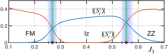
Figure S1: $|\langle S^{z}_{i}\rangle|$ and $|\langle S^{x}_{i}\rangle|$ along the length of a 16$\times$40 cylinder in a DMRG scan vs $J_{3}$ for the $\Delta\!=\!0$ limit of the $J_{1}^{\Delta}$–$J_{3}$ model. The crossing points are the phase boundaries and the shaded regions are the error bars.

II Proximity effect in the scans and the absence of an spiral phase

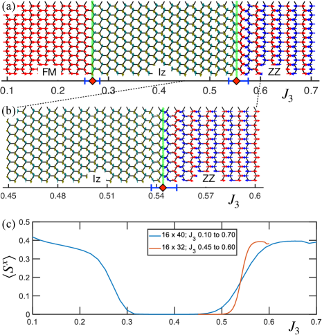
Figure S2: Results for the $J_{1}^{\Delta}$–$J_{3}$ model at $\Delta\!=\!0$. (a) The $J_{3}$-scan from Fig. 2(b) of the main text. (b) The “zoom-in” $J_{3}$-scan of the Iz-to-ZZ transition region in the 16$\times$32 cylinder. (c) The column-averaged $\langle S^{x}\rangle$ vs $J_{3}$ for the scans in (a) and (b).

In some DMRG scans, such as the one in Fig. 2(b) of the main text, reproduced in Fig. S2(a), spins at the boundary between the Iz and other phases appear to form a spiral pattern. To rule out an additional intermediate spiral phase, we perform a scan in a smaller range of the varied parameter (“zoom-in” scan) to observe the boundary region closer. In Fig. S2(b) we focus on the transition region between the Iz phase and the ZZ phase. If the spiral phase would exist, it would become wider in such a scan. In Fig. S2(b), the transition region has the same width (about ten columns) as in Fig. S2(a), with the transition getting sharper for the smaller gradient of $J_{3}$, see Fig. S2(c), strongly suggesting the absence of any intermediate phase in the thermodynamic limit. In the non-scan calculation at $J_{3}$=0.55 we also do not find the spiral phase. This analysis clearly shows that the spiral-like pattern in the scans is due to a proximity effect at the phase boundary. Similar verifications were carried out for all suspicious phases in all scans.

III Other DMRG scans for the partial XXZ $J_{1}^{\Delta}$–$J_{3}$ model

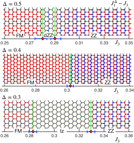
Figure S3: DMRG $J_{3}$-scans for $\Delta$=0.5, 0.4, and 0.3 in the $J_{1}^{\Delta}$–$J_{3}$ model. The scans for $\Delta$=0.5 and 0.3 are on the 12$\times$32 cylinders while the $\Delta$=0.4 scan is on the 16$\times$40 cylinder.

In Fig. S3, we show additional $J_{3}$-scans that are used to construct the phase diagram of the $J_{1}^{\Delta}$–$J_{3}$ model in Fig. 1(b) of the main text. In each scan, approximate transition boundaries with error bars are indicated. In the $\Delta\!=\!0.5$ scan, we observe a narrow phase intervening between FM and ZZ, which is identified as the dZZ phase using non-scan calculations in the region of $J_{3}$ from 0.28 to 0.29 (not shown). The $\Delta\!=\!0.4$ scan in Fig. S3 shows a direct transition from FM to ZZ. The non-scans using smaller clusters in the vicinity of $J_{3}\!=\!0.3$ have initially suggested a spin-liquid (SL) state discussed below, which turns into ZZ order in the larger non-scan clusters. The $\Delta\!=\!0.3$ scan is similar to Fig. 2(b) of the main text with an extended region of the Iz phase intervening between FM and ZZ.

IV DMRG Scans for the full XXZ $J_{1}^{\Delta}$–$J_{3}^{\Delta}$ model

In Fig. S4, we show DMRG $J_{3}$-scans that are used to construct the phase diagram of the $J_{1}^{\Delta}$–$J_{3}^{\Delta}$ model in Fig. 5 of the main text. While the $\Delta\!=\!0.5$ scan looks somewhat similar to the scan for the same $\Delta$ in Fig. S3, it has a direct FM-ZZ transition at $J_{3}\!=\!0.30$, with the separate non-scan calculations showing no sign of the intermediate phase.

In the $\Delta\!=\!0.25$ and $\Delta\!=\!0$ scans, an intermediate region is suggested with the suppressed ordered moments. As we discuss next, initial non-scans in these regions have shown strongly anisotropic correlations, with short correlations in one direction and FM-like in the other, resembling the state that has been hypothesized as a spin liquid in Ref. [1]. Upon closer inspection and finite-size scaling, they reveal a narrow region of the Iz phase. For $\Delta\!=\!0$, $J_{3}\!=\!0.33$ is in the FM phase, $J_{3}\!=\!0.37$ is in the ZZ phase, and $J_{3}\!=\!0.35$ is in the Iz phase by that analysis, confining the Iz phase between $J_{3}\!=\!0.34$ and 0.36. For $\Delta\!=\!0.25$, the Iz phase is even narrower, between $J_{3}\!=\!0.315$ and 0.325.

While the Iz phase in the $XY$ limit ($\Delta\!=\!0$) of the full $XXZ$ $J_{1}^{\Delta}$–$J_{3}^{\Delta}$ model has been suggested in Ref. [2], the $J_{3}$-width of it in our analysis is an order of magnitude narrower than in the results of the pseudo-fermion functional renormalization group method used in Ref. [2].

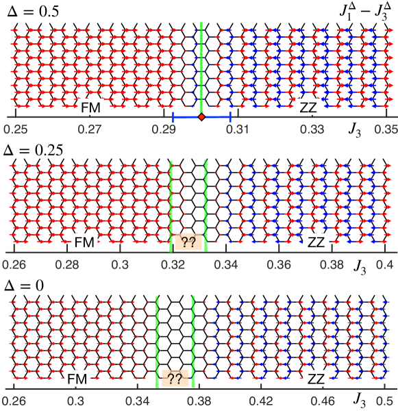
Figure S4: DMRG $J_{3}$-scans in the $J_{1}^{\Delta}$–$J_{3}^{\Delta}$ model for $\Delta$=0.5, 0.25, and 0 on the 12$\times$32 cylinders.

V Pseudo-spin-liquid state

In some of the transition regions discussed above for both versions of the $XXZ$ $J_{1}$–$J_{3}$ model, we have found regimes that can be taken as evidence for a spin-liquid state, similar to the ones reported in Ref. [1]. These include nearly zero ordered moment at intermediate bond dimension in DMRG calculations, for which the system is expected to spontaneously break symmetry if it has an order, and the short-range spin-spin correlation in one direction, as shown in Figs. S5(a) and S5(b). This anisotropy in correlations is suspicious, however, as one would expect a “lock in” of such 1D-like correlations into some order in a larger system. Indeed, with the increase of the system’s width, one of the spin-liquid possibilities in the $J_{1}^{\Delta}$–$J_{3}$ model ($\Delta\!=\!0.4$), develops a ZZ order, see Fig. S5(c).

Another such suspect region is in the $J_{1}^{\Delta}$–$J_{3}^{\Delta}$ model, $\Delta\!=\!0.25$, near $J_{3}\!=\!0.32$, similar to the one reported in Ref. [1], but it does not follow that trend. In fact, as is shown in Fig. S5(d), the spin-liquid candidate looks even more realistic (less anisotropic) in the YC lattice. However, the system was tested with various boundary conditions and responded strongly to the staggered pinning field $(-1)^{i}hS^{z}_{i}$, developing a substantial Iz order, see Fig. S5(e), with the ordered moment nearly constant $\langle S\rangle\!\approx\!0.1$ in the bulk. Following Ref. [3], we carry out an $1/L_{y}$-scaling of the ordered moment, which gives a strong indication of the Iz order in the thermodynamic limit, see Fig. S5(f).

Figure S5: (a) and (b) 12$\times$12 XC cylinder non-scans for $\Delta\!=\!0.4$ and $J_{3}\!=\!0.3$ in the $J_{1}^{\Delta}$–$J_{3}$ model showing: (a) nearly-zero ordered moment and nearest-neighbor $\langle\vec{S}_{i}\cdot\vec{S}_{i+\delta}\rangle$ (thickness of the bond), and (b) spin-spin correlation $\langle\vec{S_{i_{0}}}\cdot\vec{S_{j}}\rangle$, denoted by the length and direction of the arrow, with $i_{0}$ site shown by the green oval. The arrow on $i_{0}$ is of length 0.25. (c) Same as (a) on the 16$\times$16 cylinder. (d) Same as (b) on the 8$\times$32 YC cylinder for $\Delta\!=\!0.25$ and $J_{3}\!=\!0.32$ in the $J_{1}^{\Delta}$–$J_{3}^{\Delta}$ model. (e) Ordered moment in (d) under the Iz pinning field of 0.5 on both edges. (f) The $1/L_{y}$-scaling of the Iz ordered moment in the center of the cylinder with the edge pinning fields from (e) and the XC and YC cylinders having the aspect ratio 2, which mimics the 2D limit closely—see Ref. [3].

VI DMRG results for the $J_{1}^{\Delta}$-$J_{2}^{\Delta}$ model

Ref. [2] has studied the $J_{1}$–$J_{2}$–$J_{3}$ $XXZ$ model, demonstrating a potentially richer structure of its phase diagram compared to the $J_{1}$–$J_{3}$ model investigated in our work. Specifically, it was suggested that the spin-liquid phase in the isotropic Heisenberg limit is stable in a much wider region along the $J_{1}$–$J_{2}$ axis than along the $J_{1}$–$J_{3}$ axis, with a specific point $J_{2}\!=\!0.18$ studied in more detail. In that work, an $XXZ$ cut of the $J_{1}^{\Delta}$–$J_{2}^{\Delta}$ model along the $\Delta$-axis for $J_{2}\!=\!0.18$ (and $J_{3}\!=\!0$) was also investigated, and a transition to an incommensurate phase from an SL phase was identified near the Heisenberg limit, at $\Delta\!=\!0.96$, with a wide range of the incommensurate phase extending down to the low values of $\Delta$.

Here we briefly present our additional results for the $J_{1}^{\Delta}$–$J_{2}^{\Delta}$ model for this specific choice of $J_{2}\!=\!0.18$ and $J_{3}\!=\!0$, thus extending our work in a different region of the parameter space. The summary of our results is the following. We do not find any evidence for a spin-liquid state in the Heisenberg limit of this model, and find a double-zigzag state instead. This is similar to our results for the dZZ state in the $J_{1}$–$J_{3}$ model, found instead of the SL state suggested in Ref. [2], as is discussed in the main text. For the 1D phase diagram along the $\Delta$-axis for the same choice of $J_{2}\!=\!0.18$ and $J_{3}\!=\!0$, we find two transitions, one at $\Delta\!=\!0.93(2)$ and the other at $\Delta\!=\!0.86(2)$. The lower one is a transition to a FM state, with no sign of the incommensurate phase. While the existence of a transition at $\Delta\!=\!0.93(2)$ is, ideologically, in agreement with the transition found in Ref. [2], in our case it is between a dZZ phase and a potentially novel triple-zigzag state that also has a significant modulation of spins, characteristic of that of the spin-density wave (SDW). We refer to it as to tZZ-SDW state.

The numerical results to substantiate these findings are presented in Fig. S6. The Fig. S6(a) part shows a scan calculation at $J_{2}$=0.18 vs $\Delta$ from the Heisenberg limit down to $\Delta\!=\!0.8$. The double zigzag phase at the isotropic limit ($\Delta\!=\!1.0$) evolves into a FM state via an intermediate phase. The non-scan calculations in Fig. S6(b) and Fig. S6(d) confirm the dZZ and the FM phases at the respective ends of the scan, with both exhibiting a robust order. The non-scan for the intermediate phase at $\Delta\!=\!0.9$ in Fig. S6(c) retains the characteristics of the SDW state, as the spin’s magnitude is not varied in a fashion that would be consistent with a “simple” triple-zigzag phase. While it is possible that the SDW variation may be an artifact of the finite cluster as the tZZ phase has a large unit cell, the dZZ phase in the $J_{1}$–$J_{3}$ case is much more symmetric and we believe that the observed SDW variation is genuine.

Lastly, we note that in the energy comparison for the $J_{1}$–$J_{3}$ Heisenberg case discussed in the main text and shown in Fig. 3(b), we have also investigated a stability of the triple-ZZ state. The tZZ did come very close near the FM-dZZ boundary, but did not become the ground state in that limit. In that sense, the stabilization of the tZZ phase, or a descendant of it, in a different part of the phase diagram does not come as a complete surprise.

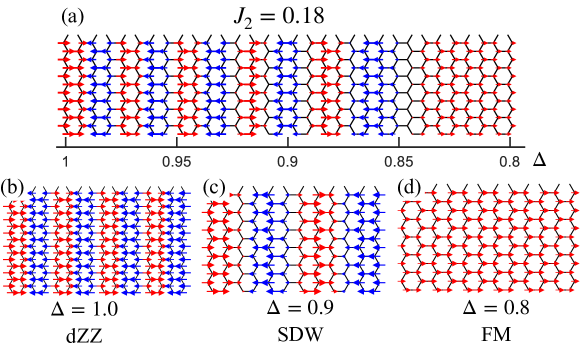
Figure S6: Results for the $J_{1}^{\Delta}$–$J_{2}^{\Delta}$ model for $J_{2}\!=\!0.18$. (a) DMRG scan on 12$\times$32 cylinder vs $\Delta$, and (b), (c), and (d) are non-scans on 16$\times$16 and 12$\times$12 cylinders for three representative values of $\Delta$.

VII generalized $J_{1}^{\Delta_{1}}$-$J_{3}^{\Delta_{3}}$ model for ${\rm BaCo_{2}(AsO_{4})_{2}}$

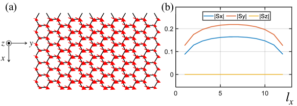
Figure S7: (a) Spin pattern in the 12$\times$12 DMRG cylinder and (b) spin components in the ground state of the generalized $XXZ$ $J_{1}^{\Delta_{1}}$-$J_{3}^{\Delta_{3}}$ model model from Ref. [4].

As is mentioned in the main text, extensive experimental and theoretical searches for the Kitaev magnets on the honeycomb lattice have recently expanded to the Co²⁺, $S_{eff}\!=\!1/2$ materials. Among this family, BaCo₂(AsO₄)₂ has received significant attention [5, 6, 7, 8, 4]. Its minimal model description has currently coalesced to a generalized $XXZ$ FM-AFM $J_{1}^{\Delta_{1}}$–$J_{3}^{\Delta_{3}}$ model [7, 8, 4, 1] with additional Kitaev-like bond-dependent terms.

One such model parametrization was advocated in Ref. [4], based on fitting experimental excitation spectrum in high fields and assuming the spin-spiral ground state with a nearly commensurate ordering ${\bf Q}$-vector in zero field. Leaving the correctness of the latter assumption aside [6], the model parameters in Ref. [4] were constrained to match the ordering ${\bf Q}$-vector of the planar spin spiral from the classical solution of the generalized $XXZ$ $J_{1}^{\Delta_{1}}$–$J_{3}^{\Delta_{3}}$ model.

Since we find that such a spiral state does not survive at all in the quantum $S\!=\!1/2$ version of the $XXZ$ $J_{1}$–$J_{3}$ model, as it is overtaken by the collinear phases due to quantum fluctuations, we have checked the validity of the key assumption made in Ref. [4] regarding the structure of the ground state for their proposed set of parameters. The model used in Ref. [4] has strong $XXZ$ anisotropies for the $J_{1}$ and $J_{3}$ terms, but of different sign, $\Delta_{1}\!=\!0.13$ and $\Delta_{3}\!=-\!0.35$, and the ratio $J_{1}/J_{3}\!=\!0.33$ (see Eq. [13] of Ref. [4]). The model also contains two minimal bond-dependent corrections in the $J_{1}$ exchange matrix.

We have performed DMRG calculations for these parameters, including the bond-dependent terms, on a 12$\times$12 cylinder in order to see whether the opposite sign of $\Delta_{1}$ and $\Delta_{3}$, or the bond-dependent terms, are able to stabilize the spiral state to avoid the fate we find for it in the other models. As is shown in Fig S7, we find an FM ground state instead of the spiral state, suggesting that the model parameters for BaCo₂(AsO₄)₂ proposed in Ref. [4] are not adequate to describe its ground-state spin configuration and require a reconsideration.

VIII Minimally augmented spin wave theory

The spin-wave approach is based on the $1/S$-expansion about a classical ground state of a spin model using bosonic representation for spin operators [9]. Since the classical energy is at a minimum, the first non-zero term of the expansion is quadratic (harmonic), yielding the liner spin-wave theory (LSWT) Hamiltonian in a standard form

$${\cal H}=E_{cl}+\frac{1}{2}\sum_{{\bf q}}\left(\hat{\bf x}_{\bf q}^{\dagger}\hat{\bf H}_{\bf q}\hat{\bf x}_{\bf q}^{\phantom{\dagger}}-\frac{1}{2}{\rm tr}(\hat{\bf H}_{\bf q})\right)+O(S^{0}),\quad\quad\hat{\bf H}_{\bf q}=\left(\begin{array}[]{cc}\hat{\bf A}^{\phantom{\dagger}}_{\bf q}&\hat{\bf B}^{\phantom{\dagger}}_{\bf q}\\[2.15277pt] \hat{\bf B}^{\dagger}_{\bf q}&\hat{\bf A}^{*}_{\bf-q}\end{array}\right),$$ (1)

where $E_{cl}$ is the classical energy, $O(S^{2})$, $\hat{\bf x}^{\dagger}_{\bf q}\!=\!\big{(}\hat{\bf a}^{\dagger}_{\bf q},\hat{\bf a}^{\phantom{{\dagger}}}_{-{\bf q}}\big{)}$ is a vector of the bosonic creation and annihilation operators, and $\hat{\bf H}_{\bf q}$ is the Hamiltonian matrix, $O(S)$, in this basis. The diagonalization of $\hat{\bf g}\hat{\bf H}_{\bf q}$, where $\hat{\bf g}$ is the diagonal para-unitary matrix, yields the LSWT magnon eigenenergies $\{\varepsilon_{1{\bf q}},\varepsilon_{2{\bf q}},\dots,-\varepsilon_{1-{\bf q}},-\varepsilon_{2-{\bf q}},\dots\}$ [10] that are guaranteed to be positive definite because the expansion is around a minimum of the classical energy.

From that, the energy of the ground state to the order $O(S)$ is ${\cal E}\!=\!E_{cl}+\delta E$, where $\delta E$ is the $1/S$ quantum correction

$$\delta E=\frac{1}{2}\sum_{\bf q}\Big{(}\sum_{\alpha}\varepsilon_{\alpha{\bf q}}-{\rm tr}(\hat{\bf A}_{\bf q})\Big{)}.$$ (2)

When the classical state stops being a minimum as some parameter of the model is varied, the quadratic Hamiltonian in (1) ceases to be positive definite, with some of the $\varepsilon_{\alpha{\bf q}}^{2}$ turning negative for some momenta ${\bf q}$, and the quantum correction in (2) becoming ill-defined. This hinders the use of the LSWT outside the classical region of stability of a state and limits its ability to describe the shift of the phase boundaries between classical states due to quantum effects and the appearance of the ordered phases that are not favored classically but stabilized in a quantum case.

The resolution to this general conundrum that has plagued application of the SWT to the classically unstable states was suggested in Refs. [11, 12, 13]. The method consists of adding a local field term to the Hamiltonian, $\delta{\cal H}\!=\!\mu\sum_{i}a^{\dagger}_{i}a_{i}$ (see the main text) and referred to as the minimally augmented SWT (MAGSWT). The minimal value of this field is chosen from the condition that all eigenvalues $\varepsilon_{\alpha{\bf q}}^{2}$ are positive definite for all the momenta ${\bf q}$.

VIII.1 LSWT for the phases of the $J_{1}$–$J_{3}$ model

The classical energies of the collinear phases of interest per number of atomic unit cells $N_{A}$ are given by

$$E_{cl}^{\rm FM}=-3S^{2}(1-J_{3}),\ \ E_{cl}^{\rm ZZ}=-S^{2}(1+3J_{3}),\ \ E_{cl}^{\rm Iz}=3S^{2}(\Delta_{1}-J_{3}\Delta_{3}),\ \ E_{cl}^{\rm dZZ}=-2S^{2},$$ (3)

valid for any $J_{3}$ and $\Delta_{1(3)}$ of the model (1) of the main text, inside or outside the phase’s stability region.

Of the five phases in Fig. 1 of the main text, the magnetic unit cell in the FM and Iz phases is naturally that of the honeycomb lattice (two sites), while for the ZZ and Sp ones it can be reduced to that by the staggered or rotated reference frames, respectively, resulting in the $4\!\times 4$ Hamiltonian LSWT matrix $\hat{\bf H}_{\bf q}$ (1) in all four cases. For the dZZ phase, the staggered reference frame reduces the unit cell from eight to four sites and yields the $8\!\times 8$ LSWT matrix.

The LSWT treatment of the collinear phases is rather standard and we do not elaborate on it except for a few details. In all two-sublattice cases, FM, ZZ, Iz, and Sp, the LSWT matrices $\hat{\bf A}_{\bf q}$, $\hat{\bf B}_{\bf q}$ in (1) assume the same structure, for which the eigenvalues of the $4\!\times 4$ Hamiltonian matrix can be found analytically. One can find additional simplifications of the eigenvalue problem for the FM and Iz phases, and in all four cases in the limit $\Delta_{1(3)}\!=\!0$, see also Ref. [14] for the limiting cases for the Sp phase.

In the 4-sublattice dZZ case, the eigenvalue problem for the $8\!\times 8$ matrix is not reducible to a compact analytical form. However, analytical solutions are available for the eigenenergies at the high-symmetry ${\bf q}\!=\!0$ and ${\bf q}\!=\!(0,\pi/\sqrt{3})$ points in the Heisenberg limit, which are instrumental for finding the MAGSWT parameter $\mu$.

VIII.2 Finding $\mu$ in MAGSWT

In the FM, ZZ, and Iz phases, the search for the minimal value of $\mu$ for the MAGSWT follows a similar pattern. In a simplified case, such as full $XXZ$ ($\Delta_{1}\!=\!\Delta_{3}$) or $XY$ limits, analytical expression for the lowest branch $\varepsilon_{1{\bf q}}^{2}$ simplifies sufficiently to yield the $J_{3}$-dependence of the offending negative minimum that needs to be lifted up by a positive shift. The required energy shift is easily related to $\mu$ with the $\Delta$-dependence of $\mu$ either absent or following trivially from the considered limiting cases. The resulting solutions correspond to a change of the diagonal matrix element $A\rightarrow\bar{A}$ of the LSWT matrix $\hat{\bf A}_{\bf q}$, with $\bar{A}$ in all three cases given by

$$\bar{A}=A+\mu=3S\left|\bar{\gamma}_{{\bf Q}_{\rm max}}\right|,\ \ \mbox{where}\ \ \bar{\gamma}_{\bf q}=\gamma_{\bf q}-J_{3}\gamma^{(3)}_{\bf q},$$ (4)

with the first- and third-neighbor hopping amplitudes $\gamma_{\mathbf{q}}=\frac{1}{3}\sum_{\alpha}e^{i\mathbf{q}{\bm{\delta}}_{\alpha}}$ and $\gamma^{(3)}_{\mathbf{q}}=\frac{1}{3}\sum_{\alpha}e^{i\mathbf{q}{\bm{\delta}}^{(3)}_{\alpha}}$, and ${\bf Q}_{\rm max}$ defined as

$${\bf Q}_{\rm max} =\left\{\begin{array}[]{ll}(0,0),&\ \ J_{3}<J_{3,c1}=0.25,\\ (Q_{x},0),\ Q_{x}=\frac{2}{3}\cdot\arccos\left(\frac{1}{2J_{3}}\cdot\frac{1-3J_{3}}{1-2J_{3}}\right),&\ \ J_{3,c1}<J_{3}<J_{3,c2},\\ (2\pi/3,0),&\ \ J_{3}>J_{3,c2}=(\sqrt{17}-1)/8\approx 0.3904,\end{array}\right.$$ (8)

Technically, the condition for the maximum of $|\bar{\gamma}_{\bf q}|$ is related to that of the classical energy minimum in the Sp phase.

Interestingly, the resultant MAGSWT spectrum in the Iz phase and the quantum energy correction (2) that derives from it, are fully independent of the anisotropy parameters $\Delta_{n}$.

In the dZZ case, the search of $\mu$ has involved analysis of the spectrum obtained by a numerical diagonalization of the $\big{(}\hat{\bf g}\hat{\bf H}_{\bf k}\big{)}^{2}$ matrix in the Heisenberg limit, which helped in identifying the relevant high-symmetry ${\bf q}$ points that require stabilization corrections. The diagonalization at these points can be reduced to an analytical form, which, in turn, yields the minimal value of $\mu$. In a narrow region of $0.1892\!<\!J_{3}\!<\!0.2030$, the two lowest unstable branches trade places and, in a row, develop negative minima at small but finite ${\bf q}$’s. For that region, we find that a straightforward linear interpolation for $\mu$ between the analytic solutions from the neighboring regions is the most effort-effective, as it stabilizes the spectrum if not with zero but with a very small gap. The resultant explicit expressions for $\mu$ are

$$\mu =\!\left\{\begin{array}[]{ll}S\left(\sqrt{5\!-\!2J_{3}\!+\!J_{3}^{2}}\!-\!1\!-\!3J_{3}\right),&J_{3}\!<\!\widetilde{J}_{c1}=0.1892,\\ \mbox{interpolate},&\widetilde{J}_{c1}\!<\!J_{3}\!<\!\widetilde{J}_{c2}=0.203,\\ 2S\left(\sqrt{2\!-\!2J_{3}\!+\!J_{3}^{2}}\!-\!1\right),&\widetilde{J}_{c2}\!<\!J_{3}\!<\!\widetilde{J}_{c3}=0.25,\\ 2SJ_{3},&J_{3}\!>\!\widetilde{J}_{c3}.\end{array}\right.$$ (13)

As in the other coplanar phases, FM and ZZ, $\mu$ is independent of the $XXZ$ anisotropies $\Delta_{n}$.

VIII.3 Energies

Following the MAGSWT strategy, quantum corrections to the groundstate energies in all competing phases can now be calculated in a conventional $1/S$ fashion using Eq. (2) with the expressions for the minimal chemical potential from (4) and (13). Then the total energies ${\cal E}(J_{3},\Delta)$ can be compared between the phases to create the phase diagram.

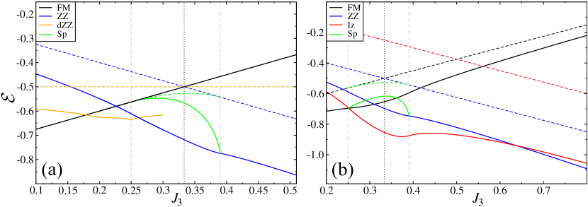
Figure S8: (a) The classical (dashed lines) and quantum (solid lines, from (2)) energies of the FM, ZZ, Sp, and dZZ states vs $J_{3}$ for $\Delta_{1(3)}\!=\!1$ per atomic unit cell. The vertical dashed lines are classical FM-Sp and Sp-ZZ boundaries and the dotted line is the crossing of $E_{cl}$ for the FM and ZZ states. (b) Same as (a) for the FM, ZZ, Sp, and Iz states for $\Delta_{1}\!=\!0$ and $\Delta_{3}\!=\!1$.

Figure S8(a) shows the $J_{3}$ energy-cuts in the Heisenberg limit, $\Delta_{1(3)}\!=\!1$, of the $J_{1}$–$J_{3}$ model. The dashed lines are classical energies (3) and solid lines are energies with quantum corrections (2). The vertical dashed lines are classical FM-Sp and Sp-ZZ boundaries, $J_{3,c1}$ and $J_{3,c2}$. The dotted line is the intersection of the FM and ZZ classical energies, $J_{3}\!=\!1/3$. The Iz phase is not competitive. The Sp phase uses standard SWT with no augmenting as it is stable through its extent. The FM is an exact eigenstate, so the quantum corrections to it are zero.

The first effect is the expansion of the ZZ phase (blue lines). While the FM is fluctuation-free, the ZZ is not, which pushes its energy down and the crossing with the FM’s energy below the $J_{3,c1}$ point where the FM is unstable classically, superseding the non-collinear Sp phase, which is not effective in lowering its energy. However, near $J_{3,c1}$ another collinear phase, dZZ, is competitive, making it a ground state in a finite range of $J_{3}$ (orange lines).

One can note a very close agreement of the MAGSWT dZZ-ZZ transition at $J_{3}\!=\!0.262$ compared to the DMRG value of 0.26. On the other hand, the FM-dZZ transition is at a lower $J_{3}\!=\!0.1785$ than the DMRG one at $J_{3}\!\approx\!0.24$. One can ascribe this difference to a larger sensitivity of the MAGSWT phase boundaries to the higher-order corrections in this case because FM state is non-fluctuating in the Heisenberg limit.

For the “partial” $XY$ limit, with $\Delta_{1}\!=\!0$ and $\Delta_{3}\!=\!1$, see Figure S8(b). In this case, dZZ is not competitive, but Iz is. All phases are fluctuating in this limit, including FM. The Sp phase is not effective in benefiting from quantum fluctuations. The transition point between FM and ZZ phase is renormalized to a slightly smaller $J_{3}$ from its classical value. However, both are overtaken by the strongly-fluctuating Iz phase in a wide window of $J_{3}$. One observation is that while the FM-Iz transition is associated with a rather steep energy crossing, the Iz-ZZ crossing is rather shallow, suggesting stronger higher-order effects on the MAGSWT phase boundary for the latter, but not the former. This is in accord with the numerical values: $J_{3}\!\approx\!0.269(15)$ [DMRG] vs 0.2513 [MAGSWT] for the FM-Iz boundary and $J_{3}\!\approx\!0.554(23)$ [DMRG] vs 0.637 [MAGSWT] for the Iz-ZZ boundary. Similar discrepancies for the finite $\Delta_{1}$ in the phase diagram in Fig. 1(b) of the main text can be attributed to the same effect.

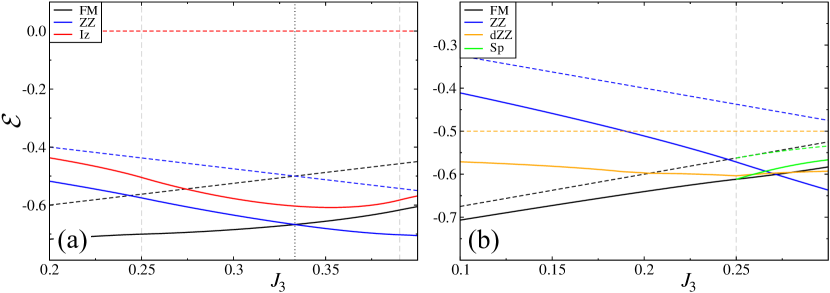
Figure S9: (a) Same as in Fig. S8(b) for the FM, ZZ, and Iz states in the “full” $XY$ limit, $\Delta_{1}\!=\!\Delta_{3}\!=\!0$. (b) Same as in Fig. S8(a) for the FM, ZZ, Sp, and dZZ states for $\Delta_{1}\!=\!0.5$ and $\Delta_{3}\!=\!1$.

We note that in the “partial” $XY$ case in Fig. S8(b), the Heisenberg $J_{3}$-term helps to stabilize the Iz state. The effect of the $\Delta_{3}$ anisotropy is tested by the “full” $XY$ limit of the model, in which the benefit of the out-of-plane spin-coupling is absent. The $J_{3}$-cut in this limit is shown in Figure S9(a). The Iz phase can be seen as remarkably effective at lowering its energy, with the quantum fluctuation part being about four times of that for the FM and ZZ states. However, while being closely competitive, the Iz phase is not stable in the full $XY$ limit according to MAGSWT. This result is, superficially, in a disagreement with the DMRG, which does show a narrow strip of the Iz phase in Fig. 5 of the main text. Nevertheless, with the energy curves in Fig. S9(a) and Fig. S8(b) in mind, it is clear that the MAGSWT misses Iz phase in the full $XY$ limit only slightly.

An additional $J_{3}$-cut for $\Delta_{1}\!=\!0.5$ and Heisenberg $J_{3}$ is shown in Fig. S9(b). Here, the competing phases are the same as in Fig. S8(a), with the dZZ phase coming extremely close, but not able to stabilize, yielding a direct FM-ZZ transition for this value of $\Delta_{1}$. This is in a close agreement with DMRG, which shows a narrow dZZ slice for $J_{3}$ between 0.280(4) and 0.290(6) at this $\Delta_{1}$, with the FM-ZZ transition being direct for the next cut at $\Delta_{1}\!=\!0.4$, see Fig. 1(b) of the main text. Given the energy differences in Fig. S9(b), the agreement is indeed very close.

Such additional insights into the energetics of the competing phases are instrumental for the understanding of their competition. They also underscore the undeniable success of the MAGSWT in describing classically unstable states.

References

- Bose et al. [2022] A. Bose, M. Routh, S. Voleti, S. K. Saha, M. Kumar, T. Saha-Dasgupta, and A. Paramekanti, Proximate Dirac spin liquid in the - model for honeycomb cobaltates, arXiv:2212.13271 (2022).
- Watanabe et al. [2022] Y. Watanabe, S. Trebst, and C. Hickey, Frustrated Ferromagnetism of Honeycomb Cobaltates: Incommensurate Spirals, Quantum Disordered Phases, and Out-of-Plane Ising Order, arXiv:2212.14053 (2022).
- White and Chernyshev [2007] S. R. White and A. L. Chernyshev, Neél Order in Square and Triangular Lattice Heisenberg Models, Phys. Rev. Lett. 99, 127004 (2007).
- Halloran et al. [2023] T. Halloran, F. Desrochers, E. Z. Zhang, T. Chen, L. E. Chern, Z. Xu, B. Winn, M. Graves-Brook, M. B. Stone, A. I. Kolesnikov, Y. Qiu, R. Zhong, R. Cava, Y. B. Kim, and C. Broholm, Geometrical frustration versus Kitaev interactions in (, Proc. Natl. Acad. Sci. U.S.A. 120, e2215509119 (2023).
- Zhong et al. [2020] R. Zhong, T. Gao, N. P. Ong, and R. J. Cava, Weak-field induced nonmagnetic state in a Co-based honeycomb, Sci. Adv. 6, eaay6953 (2020).
- Regnault et al. [2018] L.-P. Regnault, C. Boullier, and J. Lorenzo, Polarized-neutron investigation of magnetic ordering and spin dynamics in BaCo2(AsO4)2 frustrated honeycomb-lattice magnet, Heliyon 4, e00507 (2018).
- Das et al. [2021] S. Das, S. Voleti, T. Saha-Dasgupta, and A. Paramekanti, XY magnetism, Kitaev exchange, and long-range frustration in the honeycomb cobaltates, Phys. Rev. B 104, 134425 (2021).
- Maksimov et al. [2022] P. A. Maksimov, A. V. Ushakov, Z. V. Pchelkina, Y. Li, S. M. Winter, and S. V. Streltsov, Ab initio guided minimal model for the “Kitaev” material (: Importance of direct hopping, third-neighbor exchange, and quantum fluctuations, Phys. Rev. B 106, 165131 (2022).
- Holstein and Primakoff [1940] T. Holstein and H. Primakoff, Field dependence of the intrinsic domain magnetization of a ferromagnet, Phys. Rev. 58, 1098 (1940).
- Colpa [1978] J. Colpa, Diagonalization of the quadratic boson hamiltonian, Physica A: Statistical Mechanics and its Applications 93, 327 (1978).
- Wenzel et al. [2012] S. Wenzel, T. Coletta, S. E. Korshunov, and F. Mila, Evidence for Columnar Order in the Fully Frustrated Transverse Field Ising Model on the Square Lattice, Phys. Rev. Lett. 109, 187202 (2012).
- Coletta et al. [2013] T. Coletta, M. E. Zhitomirsky, and F. Mila, Quantum stabilization of classically unstable plateau structures, Phys. Rev. B 87, 060407(R) (2013).
- Coletta et al. [2014] T. Coletta, S. E. Korshunov, and F. Mila, Semiclassical evidence of columnar order in the fully frustrated transverse-field Ising model on the square lattice, Phys. Rev. B 90, 205109 (2014).
- Rastelli et al. [1979] E. Rastelli, A. Tassi, and L. Reatto, Non-simple magnetic order for simple Hamiltonians, Physica B+C 97, 1 (1979).