European Option Pricing under Generalized Tempered Stable Process: Empirical Analysis

Abstract.

The paper investigates the performance of the European option price when the log asset price follows a rich class of Generalized Tempered Stable (GTS) distribution. The GTS distribution is an alternative to Normal distribution and $\alpha$-stable distribution for modeling asset return and many physical and economic systems. The data used in the option pricing computation comes from fitting the GTS distribution to the underlying S&P 500 Index return distribution. The Esscher transform method shows that the GTS distribution preserves its structure. The extended Black-Scholes formula and the Generalized Black-Scholes Formula are applied in the study. The 12-point rule Composite Newton-Cotes Quadrature and the Fractional Fast Fourier (FRFT) algorithms were implemented and they yield the same European option price at two decimal places. Compared to the option price under the GTS distribution, the Black-Scholes (BS) model is underpriced for the Near-The-Money (NTM) and the in-the-money (ITM) options. However, the BS model and GTS European options yield the same option price for the deep out-of-the-money (OTM) and the deep-in-the-money (ITM) options.

Keywords: Generalized Tempered Stable (GTS) Distributions, Black-Scholes (BS) Model, Fractional Fourier Transform (FRFT), Equivalent Martingale Measure (EMM), Option Pricing

1. Introduction

Black-Scholes (BS) model [1] is considered the cornerstone of the option pricing theory. The model relies on the fundamental assumption that the asset returns have a normal distribution with a known mean and variance. However, based on empirical studies, the BS model model is inconsistent with a set of well-established stylized features[2]. The $\alpha$-stable distribution has been proposed [3, 4] as an alternative to the normal distribution for modeling asset return and many types of physical and economic systems. In addition to the theoretical and empirical arguments for modeling with a stable distribution, the most important argument is that the Central Limit theorem can be generalized by the stable distribution [5]. Although the stable distribution allows for varying degrees of tail heaviness and skewness, it has two major drawbacks [4]: firstly, some lack of closed formulas for density and cumulative distribution functions; secondly, most of the moments of the stable distribution are infinite. An infinite variance of the asset return leads to an infinite price for derivative instruments such as options. The Generalized Tempered Stable (GTS) distribution was developed to overcome the shortcomings of the $\alpha$-stable distribution specifically in modeling high-frequency asset returns. The tails of the GTS distribution for asset returns are heavier than the normal distribution but thinner than the stable distribution [6]. See [7, 5] For more details on Tempered Stable distribution.
There has been considerable research on the stochastic volatility model for option pricing. In the current study, we contribute to the literature by empirically investigating the European option pricing under GTS distribution. The GTS distributions form a seven-parameter family of infinitely divisible distributions, which cover several well-known subclasses like Variance Gamma distributions [8, 9], bilateral Gamma distributions [10, 7] and CGMY distributions [11]. The S&P 500 index historical data was used to fit the GTS distribution to the underlying data return distribution. The methodology is based on two computational algorithms, the Fractional Fast Fourier (FRFT) [12, 13] and twelve-point rule Composite Newton–Cotes Quadrature [14, 15].
We organize the paper as follows. We briefly present the GTS distribution’s theoretical framework in the next section. In section 3, we estimate the seven parameters of the GTS distribution from the S&P 500 index historical data. In section 4, the Equivalent Martingale Measure (EMM) is identified and computed; the Extended Black-Scholes and the Generalized Black-Scholes Formulas are provided. And the last section presents the empirical analysis of the European option price computations.

2. Generalized Tempered Stable (GTS) Process

The Lévy measure of the Generalized Tempered Stable (GTS) distribution ($V(dx)$) is defined (2.3) as a product of a tempering function ($q(x)$) (2.1) and a Lévy measure of the $\alpha$-stable distribution ($V_{stable}(dx)$)(2.2).

$$q(x) = e^{-\lambda_{+}x}\boldsymbol{1}_{x>0}+e^{-\lambda_{-}|x|}\boldsymbol{1}_{x<0}$$ (2.1)

$$V_{stable}(dx) =\left(\frac{\alpha_{+}}{x^{1+\beta_{+}}}\boldsymbol{1}_{x>0}+\frac{\alpha_{-}}{|x|^{1+\beta_{-}}}\boldsymbol{1}_{x<0}\right)dx$$ (2.2)

$$V(dx)=q(x)V_{stable}(dx) =\left(\frac{\alpha_{+}e^{-\lambda_{+}x}}{x^{1+\beta_{+}}}\boldsymbol{1}_{x>0}+\frac{\alpha_{-}e^{-\lambda_{-}|x|}}{|x|^{1+\beta_{-}}}\boldsymbol{1}_{x<0}\right)dx$$ (2.3)

where $0\leq\beta_{+}\leq 1$, $0\leq\beta_{-}\leq 1$, $\alpha_{+}\geq 0$, $\alpha_{-}\geq 0$, $\lambda_{+}\geq 0$ and $\lambda_{-}\geq 0$. These parameters play an essential role in the Levy process. $\beta_{+}$ and $\beta_{-}$ are the indexes of stability bounded below by 0 and above by 2 [16]. They capture the peakedness of the distribution in a similar way as the $\beta$-stable distribution, but the distribution tails are tempered. If $\beta$ increases (decreases), then the peakedness decreases (increases). $\alpha_{+}$ and $\alpha_{-}$ are the scale parameter, also called the process intensity [17], they determine the arrival rate of jumps for a given size. $\lambda_{+}$ and $\lambda_{-}$ control the decay rate on the positive and negative tails. Additionally, $\lambda_{+}$ and $\lambda_{-}$ are also skewness parameters. If $\lambda_{+}>\lambda_{-}$ ($\lambda_{+}<\lambda_{-}$), then the distribution is skewed to the left (right), and if $\lambda_{+}=\lambda_{-}$, then it is symmetric [5].
The GTS distribution can be denoted by $X\sim GTS(\textbf{$\beta_{+}$},\textbf{$\beta_{-}$},\textbf{$\alpha_{+}$},\textbf{$\alpha_{-}$},\textbf{$\lambda_{+}$},\textbf{$\lambda_{-}$})$ and $X=X_{+}-X_{-}$ with $X_{+}\geq 0$, $X_{-}\geq 0$. $X_{+}\sim TS(\textbf{$\beta_{+}$},\textbf{$\alpha_{+}$},\textbf{$\lambda_{+}$})$ and $X_{-}\sim TS(\textbf{$\beta_{-}$},\textbf{$\alpha_{-}$},\textbf{$\lambda_{-}$})$.

$$\int_{-\infty}^{+\infty}V(dx)=\begin{cases}+\infty&\text{if }{\beta_{+}\geq 0\vee\beta_{-}\geq 0}\\ \alpha_{+}{\lambda_{+}}^{\beta_{+}}\Gamma(-\beta_{+})+\alpha_{-}{\lambda_{-}}^{\beta_{-}}\Gamma(-\beta_{-})&\text{if }{\beta_{+}<0\wedge\beta_{-}<0}\end{cases}$$ (2.4)

From (2.4), it results that when $\beta_{+}<0$, TS($\beta_{+}$, $\alpha_{+}$,$\lambda_{+}$) is of finite activity and can be written as a Compound Poisson process on the right side ($X_{+}$). we have similar pattern when $\beta_{-}<0$. However, when $0\leq\beta_{+}\leq 1$, $X_{+}$ is an infinite activity process with infinite jumps in any given time interval. We have a similar pattern when $0\leq\beta_{-}\leq 1$. In addition to the infinite activities process, we have

$$\int_{-\infty}^{+\infty}min(1,|x|)V(dx)<+\infty$$ (2.5)

By adding the location parameter, the GTS distribution becomes GTS($\mu$, $\beta_{+}$, $\beta_{-}$, $\alpha_{+}$,$\alpha_{-}$, $\lambda_{+}$, $\lambda_{-}$) and we have:

$$Y=\mu+X=\mu+X_{+}-X_{-}\quad\quad Y\sim GTS(\mu,\beta_{+},\beta_{-},\alpha_{+},\alpha_{-},\lambda_{+},\lambda_{-})$$ (2.6)

Theorem 2.1

Consider a variable $Y\sim GTS(\textbf{$\mu$},\textbf{$\beta_{+}$},\textbf{$\beta_{-}$},\textbf{$\alpha_{+}$},\textbf{$\alpha_{-}$},\textbf{$\lambda_{+}$},\textbf{$\lambda_{-}$})$, the characteristic exponent can be written

$$\Psi(\xi)=\mu\xi i+\alpha_{+}\Gamma(-\beta_{+})\left((\lambda_{+}-i\xi)^{\beta_{+}}-{\lambda_{+}}^{\beta_{+}}\right)+\alpha_{-}\Gamma(-\beta_{-})\left((\lambda_{-}+i\xi)^{\beta_{-}}-{\lambda_{-}}^{\beta_{-}}\right)$$ (2.7)

See [10] for theorem 2.1 proof

Corollary 2.2

Let $Y=\left(Y_{t}\right)$ be a Lévy process on $\mathbb{R^{+}}$ generated by $GTS(\textbf{$\mu$},\textbf{$\beta_{+}$},\textbf{$\beta_{-}$},\textbf{$\alpha_{+}$},\textbf{$\alpha_{-}$},\textbf{$\lambda_{+}$},\textbf{$\lambda_{-}$})$.
$\forall t\in\mathbb{R^{+}}$,

$$Y_{t}\sim GTS(t\mu,\beta_{+},\beta_{-},t\alpha_{+},t\alpha_{-},\lambda_{+},\lambda_{-})$$ (2.8)

See [10] for corollary 2.2 proof

3. Parameter Estimation based on daily S&P 500 price

The Standard & Poor’s 500 Composite Stock Price Index, also known as the S&P 500, is a stock index that tracks the share prices of 500 of the largest public companies in the United States. It is used as a proxy describing the overall health of the stock market or even the U.S. economy. The daily prices were adjusted for splits and dividends. The period spans from January 04, 2010, to June 16, 2023 and the data were extracted from Yahoo Finance.

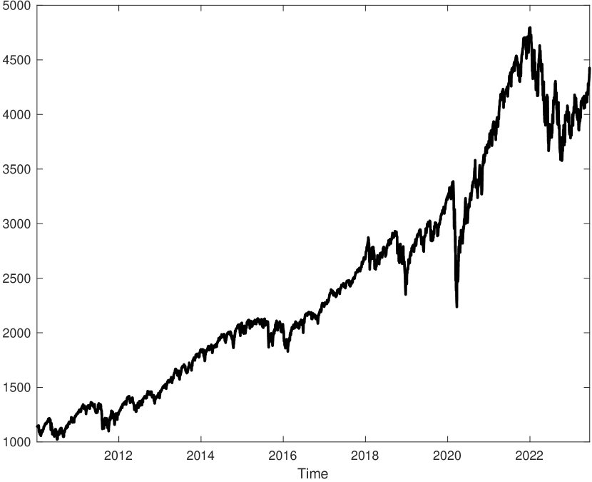
(a) S&P 500 daily price

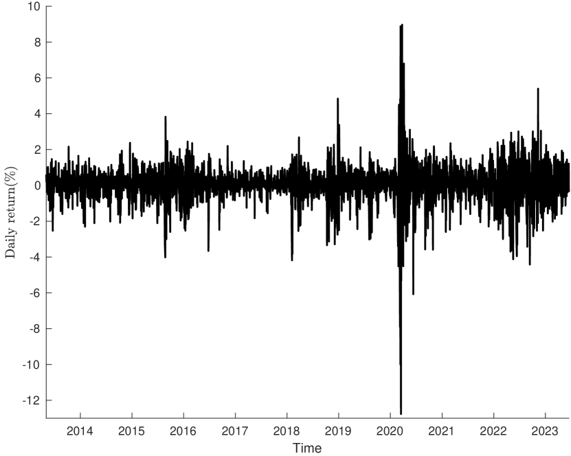
(b) S&P 500 daily Return ($\%$)

Figure 1. S&P 500 Index Historical Data

The daily price dynamics are provided in Fig 1(a) and the daily return in Fig 1(b). As shown in Fig 1(a), prices have an increasing trend throughout the period, even after the temporal disruption in the first quarter of 2020 by the coronavirus pandemic. The volatility (in Fig 1(b)) of the daily return is higher in the First quarter of 2020 amid the coronavirus pandemic and massive disruptions in the global economy.

The characteristic function of the GTS process $Y=\{Y_{t}\}$ has the following expression

$$\vartheta(\xi,t)=E\left[e^{iY_{t}\xi}\right]=e^{t\Psi(\xi)}$$ (3.1)

The GTS density function ($f$) does not have an explicit closed form or an analytical expression, which makes it challenging to utilize the density function and its derivatives and to perform the Maximum likelihood method. The GTS density function ($f$) was derived from Fourier transform ($F(f)$) as follows:

$$F[f](\xi)=\vartheta(-\xi,1)\quad\quad  f(y)=\frac{1}{2\pi}\int_{-\infty}^{+\infty}\!F[f](x)e^{iyx}\,\mathrm{d}x$$ (3.2)

The Fractional Fourier Transform (FRFT) technique was used to compute the probability density function (3.2) and its derivatives $\left\{\frac{df(y,V)}{dV_{j}}\right\}_{1\leq j\leq 7}$ and $\left\{\frac{d^{2}f(y,V)}{dV_{k}dV_{j}}\right\}_{\begin{subarray}{c}1\leq k\leq 7\\ 1\leq j\leq 7\end{subarray}}$. See [13, 9, 12] for more details on FRFT methodologies.

The results of the GTS Parameter Estimation are reported in Table 1. As expected, the stability index ($\beta$), the process intensity ($\alpha$), and the decay rate ($\lambda$) are all positive. Both stability indexes are less than 1, and capture the high peakedness of the underlying distribution. As shown in Table 1, S&P 500 return is a bit left-skewed distribution ($\lambda_{+}>\lambda_{-}$), and the right-side distribution has a high arrival rate of jumps ($\alpha_{+}>\alpha_{-}$). The higher arrival rate of jump on the right-side distribution contributes to the increased nature of the S&P 500 daily price in Fig 1(a).

Table 1. FRFT Maximum Likelihood GTS Parameter Estimations

Model	$\mu$	$\beta_{+}$	$\beta_{-}$	$\alpha_{+}$	$\alpha_{-}$	$\lambda_{+}$	$\lambda_{-}$
GTS	-0.693477	0.682290	0.242579	0.458582	0.414443	0.822222	0.727607

The Fractional Fourier Transform (FRFT) was used to estimate $(\mu,\beta_{+},\beta_{-},\alpha_{+},\alpha_{-},\lambda_{+},\lambda_{-})$ parameter. The Maximum likelihood method was applied to the density function (3.2) and the second and third derivatives were used to compute the highest eigenvalues of the hessian Matrix and the value of $||\frac{d\log(ML)}{dV}||$.
The parameter estimations of the last 30 iteration processes are shown in Table 2; in addition to the seven parameters displayed in the first row, we have added three statistical indicators: the value of the logarithmic of the product of the density functions ($\log(ML)$), the norm of the partial derivative function $||\frac{d\log(ML)}{dV}||$, and the highest value of the Eigenvalues of the Hessian matrix ($MaxEigenValue$). As shown in the last row of Table 2, the iteration process stops when the estimated parameter converges to a stable parameter with a maximum value $\log(ML)=-4659.1914$, $||\frac{d\log(ML)}{dV}||=0$ and $MaxEigenValue=-1.45426$.

Table 2. GTS Parameters Estimations for S&P 500 data

$Iterations$	$\mu$	$\beta_{+}$	$\beta_{-}$	$\alpha_{+}$	$\alpha_{-}$	$\lambda_{+}$	$\lambda_{-}$	$Log(ML)$	$||\frac{dLog(ML)}{dV}||$	$MaxEigenValue$
1	-0.5266543	0.67666185	0.43662658	0.43109407	0.32587754	0.85012595	0.60145985	-4664.7647	289.206866	48.3287566
2	-0.5459715	0.67059496	0.42415971	0.44989796	0.34810329	0.80921924	0.60289955	-4660.2156	35.9853332	-6.0431046
3	-0.7108484	0.66676659	0.20613817	0.46963149	0.41246296	0.8368645	0.73679498	-4663.5777	1082.00304	449.252496
4	-0.6704327	0.66891111	0.11250993	0.46528242	0.50028087	0.83422813	0.86330646	-4660.5268	135.684998	15.1103621
5	-0.739816	0.66779246	0.09097181	0.48302677	0.45922815	0.85551132	0.81320574	-4660.0208	45.7082317	10.8419307
6	-0.6517205	0.65580459	0.19673172	0.47996977	0.42743878	0.85248358	0.75350741	-4659.833	46.3329967	11.8534517
7	-0.8136505	0.71997129	0.21558026	0.44023152	0.41952419	0.79423596	0.74025892	-4662.4815	1187.98211	166.006596
8	-0.7805857	0.70635344	0.22952102	0.44666893	0.4166063	0.80360771	0.7334486	-4659.7758	85.6584355	-3.4305336
9	-0.7543747	0.69912144	0.23468747	0.45029318	0.41542774	0.80935861	0.73077041	-4659.1944	1.07446211	-0.7993855
10	-0.7533784	0.69885561	0.23480071	0.45042677	0.41541378	0.80956671	0.73072468	-4659.1943	1.03706137	-0.8136858
11	-0.752414	0.69859801	0.2349108	0.45055614	0.41540021	0.8097682	0.73068024	-4659.1942	1.00184387	-0.8273569
12	-0.7514794	0.69834808	0.23501796	0.45068156	0.41538701	0.80996353	0.73063702	-4659.1942	0.96860649	-0.8404525
13	-0.7496917	0.69786927	0.23522417	0.4509216	0.41536164	0.81033731	0.73055392	-4659.194	0.90739267	-0.8650984
14	-0.7471903	0.69719768	0.23551545	0.45125776	0.41532584	0.81086063	0.73043671	-4659.1938	0.82669598	-0.8987475
15	-0.7463993	0.69698491	0.23560822	0.45136413	0.41531445	0.8110262	0.73039942	-4659.1937	0.80232744	-0.9091961
16	-0.7456279	0.69677723	0.23569899	0.45146791	0.41530331	0.8111877	0.73036294	-4659.1937	0.77907591	-0.9193009
17	-0.7434222	0.69618233	0.23596025	0.45176484	0.41527126	0.81164974	0.73025805	-4659.1935	0.71530396	-0.9477492
18	-0.7427203	0.69599272	0.2360439	0.45185938	0.41526101	0.81179683	0.73022449	-4659.1934	0.69583386	-0.9566667
19	-0.7376152	0.69460887	0.23665992	0.45254797	0.41518555	0.81286777	0.72997772	-4659.193	0.56549166	-1.0197019
20	-0.7353516	0.69399264	0.23693733	0.45285383	0.41515159	0.81334323	0.72986678	-4659.1929	0.51375646	-1.0466686
21	-0.7342715	0.69369811	0.23707047	0.45299987	0.41513529	0.81357023	0.72981356	-4659.1928	0.47702329	-1.0633442
22	-0.727748	0.69191195	0.23788938	0.45388257	0.41503509	0.81494168	0.72948683	-4659.1924	0.30254549	-1.1564316
23	-0.7269375	0.69168915	0.23799284	0.45399234	0.41502243	0.81511217	0.72944561	-4659.1924	0.28659447	-1.1671214
24	-0.7261524	0.69147312	0.23809343	0.45409871	0.41501011	0.81527736	0.72940554	-4659.1923	0.27235218	-1.177299
25	-0.7074205	0.68625723	0.24059125	0.45665159	0.41470173	0.81923664	0.72841073	-4659.1916	0.15127988	-1.3705213
26	-0.7028887	0.68497607	0.24122265	0.45727561	0.4146222	0.82020261	0.72815815	-4659.1915	0.12096032	-1.4033087
27	-0.6987925	0.68381109	0.24180316	0.45784257	0.4145479	0.82107955	0.72792474	-4659.1914	0.07862954	-1.4283679
28	-0.6934505	0.68228736	0.24256739	0.45858391	0.41444901	0.82222574	0.72761631	-4659.1914	0.75324649	-1.6442249
29	-0.6934765	0.68229002	0.24257963	0.45858236	0.41444404	0.82222285	0.72760762	-4659.1914	9.93E-06	-1.4542674
30	-0.6934774	0.68229032	0.24257975	0.45858219	0.41444396	0.8222226	0.7276075	-4659.1914	7.4193E-08	-1.4542632

See [10] for more details and methodologies on Fitting GTS distribution.

4. Pricing European Options under GTS Process

4.1. GTS Process: Risk Neutral Esscher Measure

The method of Esscher transform was introduced by [18] as an efficient technique for pricing derivative securities if a Lévy process models the logarithms of the underlying asset prices. An Esscher transform of a stock-price process provides an equivalent martingale measure. The existence of the equivalent Esscher transform measure is not always guaranteed, and the issue of the unicity of the equivalent martingale measure remains recurrent when pricing an option.
From the characteristic function $\vartheta(\xi,t)$ in (3.1), the Moment generating function $M(h,t)$ of the Generalized Tempered Stable (GTS) distribution can be written as follows.

$$M(h,t)= \vartheta(-ih,t)=e^{t\Psi(-ih)}\quad\hbox{with $-\lambda_{-}<h<\lambda_{+}$}$$ (4.1)

Under the Esscher transform with parameter h, the probability density of $Y=\{Y_{t}\}$ becomes:

$$\hat{f}(x,t,h)= \frac{e^{hx}{f(x,t)}}{M(h,t)}$$ (4.2)

The Moment generating function $M(h,t)$ becomes M(z,t,h)

$$M(z,t,h)= E^{h}\left[e^{zX_{t}}\right]=\int_{0}^{+\infty}e^{zx}\hat{f}(x,t,h)dx=\left(\frac{M(h+z,1)}{M(h,1)}\right)^{t}=M(z,1,h)^{t}$$ (4.3)

$$M(z,1,h)=e^{\Psi_{h}(z)}\quad\quad\Psi_{h}(z)=\Psi(-i(h+z))-\Psi(-i(h)))$$ (4.4)

Given the process $\left\{e^{-r\tau}S(\tau)\right\}_{\tau\geq 0}$ with $r$ the constant risk-free rate of interest, we look into the conditions to have $h^{*}$ such as

$$E^{h^{*}}\left[e^{-r\tau}S(\tau)\right]=S(0)$$ (4.5)

$S(\tau)=S(0)e^{Y_{\tau}}$, with $Y_{\tau}$ is the GTS process described by the characteristic exponent (2.7). The equation (LABEL:eq:l71) becomes

$$e^{r\tau}=E^{h^{*}}\left[e^{Y_{\tau}}\right]=M(1,1,h^{*})^{\tau}=e^{\tau\Psi_{h^{*}}(1)}\quad\quad\Psi_{h^{*}}(1)=r\quad\hbox{ with $-\lambda_{-}<h^{*}<\lambda_{+}$ }$$ (4.6)

The existence and unicity of $h^{*}$ in (4.10) were studied empirically using the parameter data from Table 1. Over the interval $]-\lambda_{-};\lambda_{+}[$, $\Psi_{h}(1)$ is a strictly increasing function, as shown in Fig 2(a). Fig 2(b) provides the solution $h^{*}$ of equation (4.10) for free interest rate less than 10%. The solution $h^{*}$ increases with free interest rate $r$.

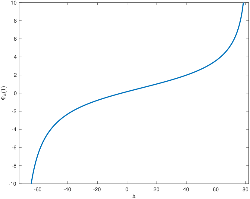
(a) $\Psi_{h}(1)$

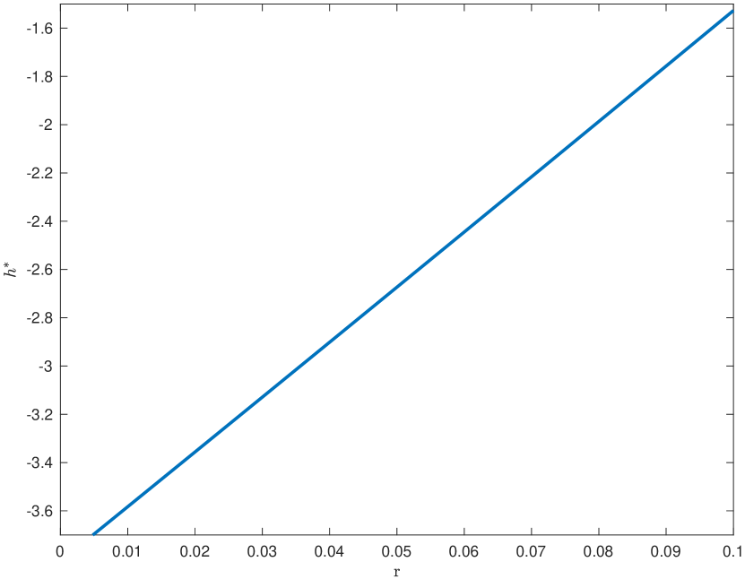
(b) $\Psi_{h^{*}}(1)=r$

Figure 2. $\mu=-0.693477$, $\beta_{+}=0.682290$, $\beta_{-}=0.242579$, $\alpha_{+}=0.458582$, $\alpha_{-}=0.414443$, $\lambda_{+}=0.822222$, $\lambda_{-}=0.727607$

Theorem 4.1

(GTS Esscher transform distribution)
Esscher transform of GTS process $Y=\{Y_{t}\}_{t\geq 0}$ with parameter $(t\mu,\beta_{+},\beta_{-},t\alpha_{+},\alpha_{-},\lambda_{+},\lambda_{-})$ is also a is also a GTS process $Y^{*}=\{Y^{*}_{t}\}_{t\geq 0}$ with parameter $(t\mu,\beta_{+},\beta_{-},t\alpha_{+},t\alpha_{-},\tilde{\lambda}_{+},\tilde{\lambda}_{-})$

$$\tilde{\lambda}_{+}=\lambda_{+}-h^{*}\quad\quad\tilde{\lambda}_{-}=\lambda_{-}+h^{*}$$ (4.7)

Proof.

we recall the function $\Psi_{h^{*}}(z)$ in (4.4).

$$\Psi_{h^{*}}(z) =\Psi(-i(h^{*}+z))-\Psi(-i(h^{*})))$$ (4.8)

$$=\mu z+\alpha_{+}\Gamma(-\beta_{+})\left(((\lambda_{+}-h^{*})+z)^{\beta_{+}}-{(\lambda_{+}-h^{*})}^{\beta_{+}}\right)+$$

$$\alpha_{-}\Gamma(-\beta_{-})\left(((\lambda_{-}+h^{*})+z)^{\beta_{-}}-{(\lambda_{-}+h^{*})}^{\beta_{-}}\right)$$

Using the Esscher transform method, the moment generating function for GST process $Y=\{Y_{t}\}_{t\geq 0}$ becomes:

$$M(z,t,{h^{*}})= E^{{h^{*}}}\left[e^{zY_{t}}\right]=M(z,1,{h^{*}})^{t}=e^{t\Psi_{h^{*}}(z)}\quad \hbox{with $-\lambda_{-}-h^{*}\leq z\leq\lambda_{+}-h^{*}$ }$$ (4.9)

The Esscher transform method preserves the structure of the GTS process. We have a new GST process generated by the GST distribution $GST(\mu,\beta_{+},\beta_{-},\alpha_{+},\alpha_{-},\lambda_{+}-h^{*},\lambda_{-}+h^{*})$. ∎

4.2. Extended Black-Scholes Formula

Under the EMM, $f(\xi,\tau,h^{*})$ is the probability density of GST distribution with parameter
$(\tau\mu,\beta_{+},\beta_{-},\tau\alpha_{+},\tau\alpha_{-},\tilde{\lambda}_{+},\tilde{\lambda}_{-})$. ($\tilde{\lambda}_{+},\tilde{\lambda}_{-}$) is defined in (4.7).

Corollary 4.2

(Extended Black-Scholes) 
Let $r$ a continuously compounded risk-free rate of interest; $Y=\{Y_{t}\}_{t\geq 0}$, a GST Process with parameter $(t\mu,\beta_{+},\beta_{-},t\alpha_{+},t\alpha_{-},\tilde{\lambda}_{+},\tilde{\lambda}_{-})$; and $(S(0)e^{X_{T}}-K)^{+}$ the terminal payoff for a contingent claim with the expiry date $T$. Then at time $t<T$, the arbitrage price of the European call option with the strike price $K$ can be written as follows.

$$F^{GTS}_{call}(S_{t},t) =S(t)\left[1-F(log(\frac{K}{S(t)}),\tau,h^{*}+1)\right]-Ke^{-r\tau}\left[1-F(log(\frac{K}{S(t)}),\tau,h^{*})\right]$$ (4.10)

$$F(log(\frac{K}{S(t)}),\tau,h^{*})=\int_{-\infty}^{log(\frac{K}{S(t)})}f(\xi,\tau,h^{*})d\xi$$ (4.11)

Where $\tau=T-t$, $F(k,\tau,h^{*})$ and $F(k,\tau,h^{*}+1)$ are the cumulative distribution of GST distribution.

See [9] for corollary 4.2 proof

The GTS distribution function’s probability density and cumulative functions were obtained through the inverse Fourier transform. See [13, 12, 9] for details.

$$f(\xi,\tau,h^{*})=\frac{1}{2\pi}\int_{-\infty}^{+\infty}e^{i\xi z+\tau\Psi_{h^{*}}(-z)}dz\quad\quad F(\xi,\tau,h^{*})=\frac{1}{2\pi}\int_{-\infty}^{+\infty}\frac{e^{i\xi z+\tau\Psi_{h^{*}}(-z)}}{iz}dz+\frac{1}{2}$$ (4.12)

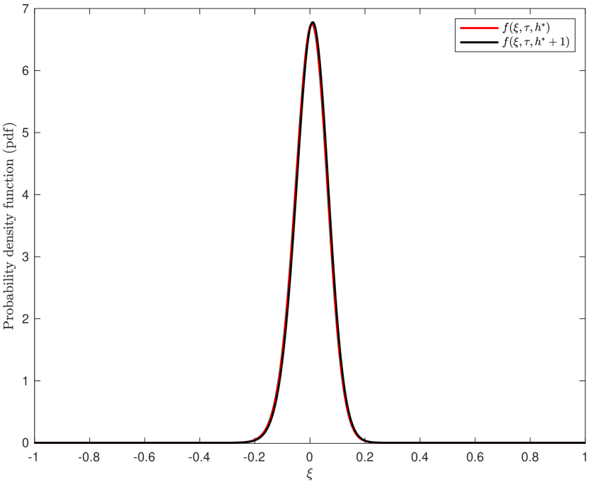
(a) $\tau=\frac{1}{12}$ years

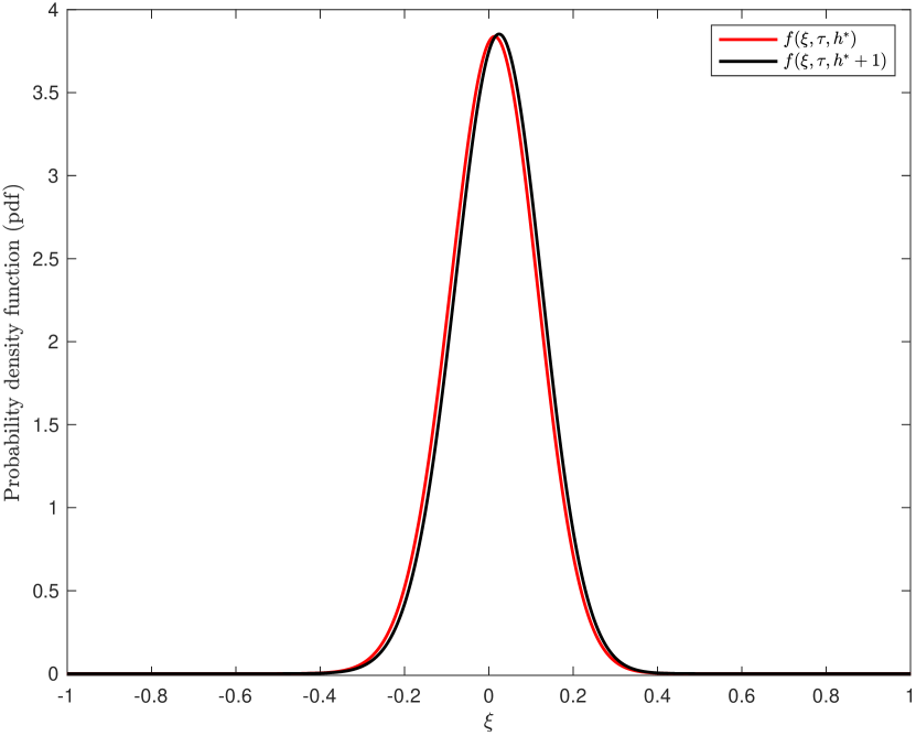
(b) $\tau=0.25$ years

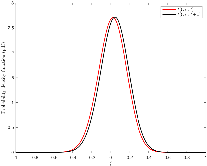
(c) $\tau=0.5$ years

Figure 3. Estimations: $f(\xi,\tau,h^{*})$ versus $f(\xi,\tau,h^{*}+1)$

Based on parameter data from Table 1, we added a 6% risk-free interest rate and the corresponding Esscher transform parameter ($h^{*}=-2.4448$) in Fig 2(b). FRFT technique was used to compute the density and cumulative functions in (4.12).

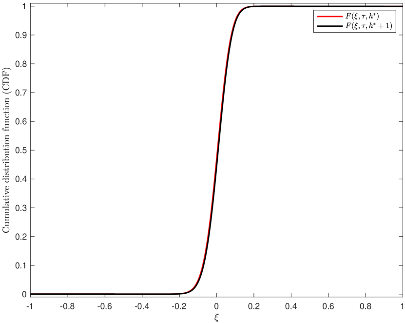
(a) $\tau=\frac{1}{12}$ years

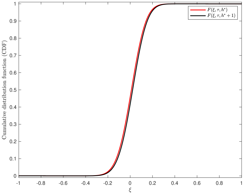
(b) $\tau=0.25$ years

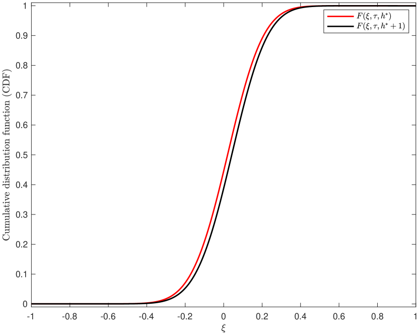
(c) $\tau=0.5$ years

Figure 4. Estimations: $F(\xi,\tau,h^{*})$ versus $F(\xi,\tau,h^{*}+1)$

As shown in Fig 3 and 4, the discrepancy between both functions increases with the period ($\tau$). The estimation results will be used to compute the option pricing (4.11).

4.3. Generalized Black-Scholes Formula

Under the EMM, $f(\xi,\tau,h^{*})$ can be written as follows:

$$f(\xi,\tau,h^{*})=\frac{1}{2\pi}\int_{-\infty}^{+\infty}e^{-i\xi z-\tau\varphi(z)}dz\quad\quad\varphi(z)=-\Psi_{h^{*}}(z)$$ (4.13)

with $\Psi_{h^{*}}(z)$ defined in (4.3).

Theorem 4.3

Let $r$ a continuously compounded risk-free rate of interest; $Y=\{Y_{t}\}_{t\geq 0}$, a Variance-Gamma Process with parameter $(\mu t,\delta,\sigma,\alpha t,\theta)$; and $(S(0)e^{X_{T}}-K)^{+}$, the terminal payoff for a contingent claim with the expiry date $T$. Then at time $t<T$, the arbitrage price of the European call option with the strike price $K$ can be written as follows.

$$F^{GTS}_{call}(S_{t},t)=\frac{K}{2\pi}\int_{-\infty+iq}^{+\infty+iq}{\frac{e^{\left(i\xi log(\frac{S(t)}{K})-\tau(r+\varphi(\xi))\right)}}{i\xi(i\xi-1)}d\xi}$$ (4.14)

Where $\varphi(z)$ is the characteristic exponent of the VG model, $\tau=T-t$, and $q<-1$.

See [9] for theorem 4.3 proof

To compute $F^{GTS}_{call}$ in (4.14), the numerical integration technique, called the Newton-Cotes formula of 12 degrees, will be implemented as follows.

$$g^{x}(\xi)=\frac{exp\left[{i(\xi+iq)x-\tau(r-\Psi_{h^{*}}(\xi+iq))}\right]}{2\pi i(\xi+iq)(i(\xi+iq)-1)}\quad\widehat{F^{GTS}_{call}}=\frac{b}{n}\sum_{p=0}^{\frac{n}{Q}-1}\sum_{j=0}^{Q}W_{j}g^{log(\frac{S(t)}{K})}(\xi_{Qp+j})$$ (4.15)

In order to perform the integral (4.15), the following parameter values were used: $a=0$, $b=20$, $Q=12$, $n=5000Q$, $n_{0}=5000$. See [15, 14, 19] for more details on the choice of parameter values and the twelve-point rule Composite Newton–Cote’s methodology.

4.4. Parameter $q$ Evaluation

Let us consider the stock or index price $S=S_{0}e^{Y}$ and the strike price $K$; the call payoff can be written as follows.

$$(S(0)e^{Y_{T}}-K)^{+} =S(t)(e^{Y_{\tau}}-k)^{+}=S(t)g(Y_{\tau},k)\ \ \ \ k=\frac{K}{S_{t}}$$ (4.16)

The Fourier transform of the call payoff in (4.16) can be derived as follows

$$\mathscr{F}[g](y,k) =\int_{0}^{+\infty}e^{-iyx}g(x,k)dx=\frac{ke^{-iylog(k)}}{iy(iy-1)}\quad \hbox{for $\Im(y)<-1$}$$ (4.17)

Call payoff in (4.16) can be recovered from the inverse of Fourier and labeled $\check{g}(x,k)$ with

$$\check{g}(x,k)=\frac{1}{2\pi}\int_{-\infty+iq}^{+\infty+iq}e^{iyx}\mathscr{F}[g](y,k)dy\hskip 14.22636pt \hbox{for $q<-1$}$$ (4.18)

The payoff ($\check{g}(x,k)$) in (4.18) depends on the $q$ parameter as shown in Fig 5(a). The inverse Fourier ($\check{g}(x,k)$) produces poor results if $q=-2$ (color red).

To find the $q$ value with a high level of accuracy, we define the error function ($ER(k,q)$) between the call payoff in (4.16) and the inverse Fourier payoff in (4.18).

$$ER(k,q)=\sqrt{\frac{1}{m}\sum_{j=1}^{m}\left[(e^{x_{j}}-k)^{+}-\check{g}(x_{j},k)\right]^{2}}\hskip 14.22636pt \hbox{with $-M\leq x_{j}\leq M$}$$ (4.19)

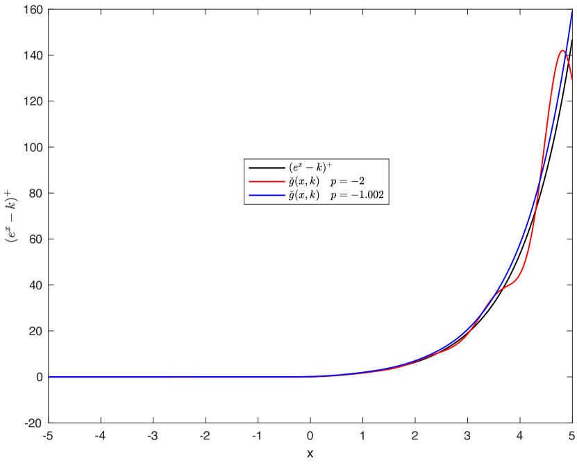
(a) $(X-k)^{+}$ versus $\check{g}(x,k)$

(b) $ER(k,q)$ and Optimal parameter (q)

Figure 5. Optimal parameter ($q$) and minimum Error value ($ER(k,q)$)

Fig 5(b) displays (in color blue) the $ER(k,q)$ minimum value as a function of the strike price $k$; and the optimal correspondent parameter $q$ as a function of the strike price $k$ (in color red). Both graphs display almost a constant function with respect to the strike price.

5. Empirical Analysis: A case of S&P 500 return

Based on parameter data from Table 1, we added a 6% risk-free interest rate and the corresponding Esscher transform parameter ($h^{*}=-2.4448$) in Fig 2(b). The GTS option pricing will be computed across maturity and option moneyness using Extended and Generalized Black-Scholes formulas. The closed-form Black-Scholes model [20] was added to the analysis as a benchmark.

$$F^{BS}_{call}(S_{t},\tau) =S_{t}N(d_{1})-Ke^{-r\tau}N(d_{2})$$ (5.1)

$$d_{1}=\frac{Ln(\frac{S_{t}}{K})+(r+\frac{1}{2}\sigma^{*2})\tau}{\sigma^{*}\sqrt{\tau}}\quad\quad d_{2} =d_{1}-\sigma^{*}\sqrt{\tau}\quad\quad N(x)=\frac{1}{\sqrt{2\pi}}\int_{-\infty}^{x}\exp\left(-\frac{t^{2}}{2}\ \right)\,dt$$ (5.2)

The variance $\sigma^{*}=0.1848$ is the annualized variance computed from the variance in Table 2.
Moneyness describes the intrinsic value of an option in its current state, which indicates whether the option would make money if exercised immediately. Option moneyness can be classified into three categories: At-the-money (ATM) option ($k=\frac{S_{t}}{K}=1$), Out-of-the-money (OTM) option ($k=\frac{S_{t}}{K}<1$), and In-the-money (ITM) option ($k=\frac{S_{t}}{K}>1$).
On August 15, 2023, the S&P 500 market price closed at $\$4,437.86$. We compute the GTS call option price on S&P 500 with the spot price ($S_{0}$) $\$4,437.86$. Table 3 summarizes the price computations as a function of time to maturity ($\tau$) and option moneyness ($k=\frac{S_{t}}{K}$).

Table 3. European Call Price on S&P 500

Strike Price	Moneyness($\frac{S_{t}}{K}$)	BSM	GTS(4.14)	GTS(4.7)	BSM	GTS(4.14)	GTS(4.7)	BSM	GTS(4.14)	GTS(4.7)	BSM	GTS(4.14)	GTS(4.7)	BSM	GTS(4.14)	GTS(4.7)	BSM	GTS(4.14)	GTS(4.7)
Period ( in year)		0.0625			0.125			0.25			0.5			0.75			1
2,689.61	1.65	1,758.315	1,758.320	1,758.315	1,768.345	1,768.349	1,768.345	1,788.291	1,788.296	1,788.291	1,827.756	1,827.782	1,827.776	1,866.803	1,866.905	1,866.898	1,905.614	1,905.833	1,905.826
2,773.66	1.60	1,674.579	1,674.584	1,674.579	1,684.922	1,684.927	1,684.922	1,705.492	1,705.498	1,705.493	1,746.215	1,746.258	1,746.252	1,786.624	1,786.778	1,786.772	1,826.924	1,827.229	1,827.221
2,863.14	1.55	1,585.441	1,585.445	1,585.441	1,596.118	1,596.122	1,596.118	1,617.352	1,617.359	1,617.354	1,659.443	1,659.517	1,659.511	1,701.402	1,701.634	1,701.628	1,743.414	1,743.833	1,743.826
2,958.57	1.50	1,490.361	1,490.364	1,490.361	1,501.393	1,501.397	1,501.393	1,523.336	1,523.347	1,523.343	1,566.952	1,567.080	1,567.075	1,610.728	1,611.072	1,611.066	1,654.742	1,655.312	1,655.305
3,060.59	1.45	1,388.723	1,388.726	1,388.723	1,400.135	1,400.140	1,400.136	1,422.842	1,422.865	1,422.861	1,468.225	1,468.444	1,468.439	1,514.200	1,514.700	1,514.695	1,560.590	1,561.354	1,561.347
3,169.90	1.40	1,279.825	1,279.828	1,279.825	1,291.645	1,291.650	1,291.647	1,315.189	1,315.242	1,315.238	1,362.746	1,363.110	1,363.105	1,411.460	1,412.173	1,412.167	1,460.696	1,461.702	1,461.695
3,287.30	1.35	1,162.861	1,162.864	1,162.861	1,175.120	1,175.130	1,175.127	1,199.631	1,199.756	1,199.752	1,250.063	1,250.643	1,250.638	1,302.261	1,303.246	1,303.241	1,354.907	1,356.202	1,356.196
3,413.74	1.30	1,036.899	1,036.903	1,036.900	1,049.637	1,049.670	1,049.667	1,075.413	1,075.692	1,075.688	1,129.906	1,130.791	1,130.786	1,186.555	1,187.872	1,187.867	1,243.245	1,244.872	1,244.866
3,550.29	1.25	900.861	900.871	900.869	914.166	914.285	914.282	941.956	942.524	942.521	1,002.394	1,003.666	1,003.663	1,064.634	1,066.328	1,066.323	1,126.008	1,127.992	1,127.986
3,698.22	1.20	753.494	753.552	753.550	767.731	768.107	768.105	799.315	800.337	800.335	868.330	870.037	870.033	937.303	939.382	939.378	1,003.876	1,006.213	1,006.208
3,859.01	1.15	593.480	593.800	593.799	610.219	611.153	611.152	649.077	650.650	650.648	729.588	731.693	731.690	806.084	808.496	808.492	878.047	880.690	880.686
4,034.42	1.10	420.919	422.039	422.037	444.934	446.566	446.564	495.718	497.690	497.687	589.513	591.851	591.848	673.405	676.021	676.016	750.358	753.204	753.199
4,226.53	1.05	245.429	247.061	247.060	283.281	284.940	284.939	347.774	349.635	349.633	453.122	455.394	455.391	542.703	545.313	545.310	623.363	626.252	626.249
4,437.86	1.00	100.299	100.154	100.153	146.757	147.206	147.205	217.356	218.448	218.447	326.853	328.694	328.692	418.344	420.686	420.683	500.326	503.053	503.049
4,671.43	0.95	23.028	21.981	21.981	56.504	55.743	55.743	116.478	116.527	116.526	217.593	218.712	218.711	305.239	307.061	307.059	385.051	387.398	387.395
4,930.96	0.90	2.309	2.146	2.146	14.527	13.845	13.845	51.103	50.510	50.510	130.982	131.319	131.318	208.118	209.260	209.259	281.521	283.307	283.305
5,221.01	0.85	0.078	0.090	0.090	2.209	2.034	2.034	17.375	16.800	16.800	69.543	69.311	69.311	130.530	130.995	130.994	193.324	194.458	194.456
5,547.33	0.80	0.001	0.002	0.002	0.173	0.163	0.163	4.290	4.021	4.021	31.596	31.153	31.153	73.869	73.823	73.822	122.955	123.470	123.469
5,917.15	0.75	0.000	0.000	0.000	0.006	0.007	0.007	0.712	0.645	0.646	11.837	11.474	11.474	36.829	36.533	36.533	71.172	71.223	71.222
6,339.80	0.70	0.000	0.000	0.000	0.000	0.000	0.000	0.072	0.064	0.064	3.493	3.304	3.304	15.702	15.392	15.392	36.685	36.488	36.488
6,827.48	0.65	0.000	0.000	0.000	0.000	0.000	0.000	0.004	0.004	0.004	0.767	0.702	0.703	5.514	5.310	5.310	16.377	16.132	16.132
7,396.43	0.60	0.000	0.000	0.000	0.000	0.000	0.000	0.000	0.000	0.000	0.116	0.103	0.103	1.520	1.428	1.428	6.111	5.932	5.932
8,068.84	0.55	0.000	0.000	0.000	0.000	0.000	0.000	0.000	0.000	0.000	0.011	0.009	0.009	0.309	0.281	0.281	1.819	1.729	1.729

(4.14): 12-point rule Composite Newton-cotes Quadrature     (4.7): FRFT-CDF

The Fractional Fourier Transform (FRFT) algorithm is used to perform the GTS cumulative function in the extended Black-Scholes formula (4.7), whereas the twelve-point rule Composite Newton–Cotes Quadrature algorithm is used to perform the Generalized Black-Scholes Formula (4.14). As expected, both algorithms produce the same estimation for European option prices at two decimal places.
To generalize the analysis and account for a large range of option moneyness and maturity, The error (5.3) was computed as the difference between VG and BS option prices:

$$Error(k,\tau)=\frac{F^{GTS}_{call}(S_{t},\tau)}{K}-\frac{F^{BS}_{call}(S_{t},\tau)}{K}\quad\quad\hbox{$(k=\frac{S_{t}}{K})$}$$ (5.3)

Fig 6 displays the error ($Error(k,\tau)$) as a function of the time to maturity ($\tau$) and the option moneyness ($k$). The spot price ($S_{t}$) is a constant, and the option moneyness depends on the strike price. The Black-Scholes (BS) model and GTS European option produce different pricing results. Compared to the option price under the GTS distribution, the BS model is underpriced for the at-the-money (ATM) and the in-the-money (ITM) options as shown in Fig 6.

(a) Error(k,$\tau$)

(b) Error(k,$\tau$) (top view)

Figure 6. Combined Effects of time to Maturity and Option Moneyness

For the out-the-money (OTM) option, the Black-Scholes (BS) model is slightly overpriced (dark blue color in Fig 6). However, the BS model and GTS European options yield the same option price for the deep out-of-the-money (OTM) and the deep-in-the-money (ITM) options.
The findings can be compared to the European option pricing under the Variance-Gamma process [9, 21]. In both studies, we have the same pattern. the BS model is underpriced for the in-the-money (ITM) option, whereas the BS model is overpriced for the out-the-money (ITM) option. However, The error ($Error(k,\tau)$) between the BS model and GTS European options has a slightly different magnitude compared to the magnitude error($Error(k,\tau)$) between the BS model and option pricing under the Variance-Gamma process [9].

6. Conclusion

The paper examines the pricing of the European option when the log asset price follows a rich class of Generalized Tempered Stable (GTS) distribution. The S&P 500 data is used to illustrate the pricing results. The Equivalent Martingale Measure (EMM) of the GTS distribution exists, and the Esscher transform method preserves the structure of the GTS distribution.
The extended Black-Scholes formula was computed based on the cumulative distribution function (CDF) generated by the Fractional Fast Fourier (FRFT) algorithms. In addition, The Generalized Black-Scholes Formula was computed using the 12-point rule Composite Newton-Cotes Quadrature algorithms. Both algorithms yield the same European option price at two decimal places.
The Black-Scholes (BS) model and GTS European options produce different pricing results. Compared to the option price under the GTS distribution, the BS model is underpriced for the near-the-Money (NTM) and the in-the-money (ITM) options. However, BS model and GTS European options yield the same option price for the deep out-of-the-money (OTM) and the deep-in-the-money (ITM) options.

References

- [1] Fischer Black and Myron Scholes. The pricing of options and corporate liabilities. Journal of Political Economy, 81(3):637–654, 1973.
- [2] R. Cont. Empirical properties of asset returns: stylized facts and statistical issues. Quantitative Finance, 1(2):223–236, feb 2001.
- [3] Sato Ken-Iti. Lévy processes and infinitely divisible distributions. Cambridge university press, 1999.
- [4] John P Nolan. Models for Heavy Tailed Data. Springer, 2020.
- [5] Svetlozar T Rachev, Young Shin Kim, Michele L Bianchi, and Frank J Fabozzi. Financial models with Lévy processes and volatility clustering, volume 187. John Wiley & Sons, 2011.
- [6] Michael Grabchak and Gennady Samorodnitsky. Do financial returns have finite or infinite variance? a paradox and an explanation. Quantitative Finance, 10(8):883–893, 2010.
- [7] Uwe Küchler and Stefan Tappe. Tempered stable distributions and processes. Stochastic Processes and their Applications, 123(12):4256–4293, 2013.
- [8] Dilip B Madan, Peter P Carr, and Eric C Chang. The variance gamma process and option pricing. Review of Finance, 2(1):79–105, 1998.
- [9] A H Nzokem. Pricing european options under stochastic volatility models: Case of five-parameter variance-gamma process. Journal of Risk and Financial Management, 16(1), 2023.
- [10] A. H. Nzokem and V. T. Montshiwa. Fitting generalized tempered stable distribution: Fractional fourier transform (frft) approach. ARXIV.2205.00586[q-fin.ST], 2022.
- [11] Peter Carr, Hélyette Geman, Dilip B Madan, and Marc Yor. Stochastic volatility for lévy processes. Mathematical finance, 13(3):345–382, 2003.
- [12] A H Nzokem. Gamma variance model: Fractional fourier transform (FRFT). Journal of Physics: Conference Series, 2090(1):012094, nov 2021.
- [13] A. H. Nzokem. Fitting infinitely divisible distribution: Case of gamma-variance model, 2021.
- [14] A H Nzokem. Numerical solution of a gamma - integral equation using a higher order composite newton-cotes formulas. Journal of Physics: Conference Series, 2084(1):012019, nov 2021.
- [15] A H Nzokem. Stochastic and Renewal Methods Applied to Epidemic Models. PhD thesis, York University , YorkSpace institutional repository, 2020.
- [16] Szymon Borak, Wolfgang Härdle, and Rafał Weron. Stable distributions. In Statistical tools for finance and insurance, pages 21–44. Springer, 2005.
- [17] Svetlana Boyarchenko and Sergei Z Levendorskii. Non-Gaussian Merton-Black-Scholes Theory, volume 9. World Scientific, 2002.
- [18] Hans U Gerber, Elias SW Shiu, et al. Option pricing by Esscher transforms. HEC Ecole des hautes études commerciales, 1993.
- [19] A H Nzokem. Sis epidemic model: Birth-and-death markov chain approach. International Journal of Statistics and Probability, 10(4):10–20, July 2021.
- [20] John C Hull. Options futures and other derivatives. Pearson Education India, 2003.
- [21] Sharif Mozumder, Ghulam Sorwar, and Kevin Dowd. Revisiting variance gamma pricing: An application to s&p500 index options. International Journal of Financial Engineering, 2(02):1550022, 2015.