Exploiting Symmetry and Heuristic Demonstrations in Off-policy Reinforcement Learning for
Robotic Manipulation

Abstract

Reinforcement learning demonstrates significant potential in automatically building control policies in numerous domains, but shows low efficiency when applied to robot manipulation tasks due to the curse of dimensionality. To facilitate the learning of such tasks, prior knowledge or heuristics that incorporate inherent simplification can effectively improve the learning performance. This paper aims to define and incorporate the natural symmetry present in physical robotic environments. Then, sample-efficient policies are trained by exploiting the expert demonstrations in symmetrical environments through an amalgamation of reinforcement and behavior cloning, which gives the off-policy learning process a diverse yet compact initiation. Furthermore, it presents a rigorous framework for a recent concept and explores its scope for robot manipulation tasks. The proposed method is validated via two point-to-point reaching tasks of an industrial arm, with and without an obstacle, in a simulation experiment study. A PID controller, which tracks the linear joint-space trajectories with hard-coded temporal logic to produce interim midpoints, is used to generate demonstrations in the study. The results of the study present the effect of the number of demonstrations and quantify the magnitude of behavior cloning to exemplify the possible improvement of model-free reinforcement learning in common manipulation tasks. A comparison study between the proposed method and a traditional off-policy reinforcement learning algorithm indicates its advantage in learning performance and potential value for applications.

I Introduction

Over the last decade, innovation in industrial manufacturing has tremendously benefitted from the introduction of artificial intelligence (AI) leading to improved the efficiency, flexibility, and transferability of the manufacturing processes. As robots are the most widely applied executional components in manufacturing, intelligentization of robotic systems is therefore one of the most important subjects to realize applied intelligent manufacturing. Reinforcement Learning (RL) provides a feasible solution for intelligent planning and control of robotic systems [1, 2]. The general function of deep RL is to use a universal approximator, usually an artificial neural network, to construct the robot control policy that regulates the robot motion given the observed robot system states. Different from the conventional control programs which are fixed for specific tasks and scenes, such as control [3, 4] and fault diagnosis [5, 6], an RL program, or agent, is designed as a parameterized structure which can be automatically tuned using the interaction data collected during the robot task execution process. This indicates that an RL-powered robot program does not require the experts to specify the patterns for every possible task. Instead, it can formulate its own knowledge and learn the feasible policy automatically while interacting with the environment. A typical example is the end-to-end visuomotor learning scheme, where a deep neural network is used as a policy network to directly map the machine perception input to the desired robot motion [7, 8]. The parameters of the policy network are trained through the interaction data.

A major limitation of RL training is its low sampling inefficiency [9, 10], that limits real-world applications. Often, a tremendous amount of data is required for a bootstrapped policy to achieve theoretical stochastic optimality. While only very little amount of this data is beneficial for the actual policy improvement. Thus, the training of an RL agent is usually temporally and computationally expensive, especially for robot manipulation tasks given the high dimensional search spaces. In this sense, an end-to-end learning scheme with minimal heuristics is not practical for robotic engineering. In fact, appropriate selection of heuristics can leverage the effort of the agent training and improve the training efficiency by properly incorporating expert knowledge. For example, state representation learning is used to provide additional feature-extraction layers for the vision-based end-to-end learning schemes to reduce the scale of the policy search space [11, 12]. Also, more attention has been attracted by hierarchical reinforcement learning (HRL), a heuristic layer-based structure that decouples a complicated task into several simpler tasks subjected to different layers in a hierarchical fashion. Then, a simple agent is trained for each layer with smaller spaces and less complicated configurations. HRL-based methods have been applied to various robot manipulation tasks, such as grasping [13], navigation [14], assembly [15], and block-stacking [16]. Similarly, a curriculum over the state space can be applied to the training process to improve training of complex tasks [17, 18]. Meanwhile, the dynamic movement primitive (DMP) provides a heuristic model to facilitate stable robot control such that more attention can be focused on safety and successful rate of the robot tasks [19]. All these schemes can significantly reduce the unnecessary exploration in the policy space and improve the RL agent training by imposing proper heuristics.

Without changing the agent structure, another two types of heuristics commonly used to improve the efficiency of RL are symmetry and demonstrations. Symmetry is described as an abstract of the environment model with which different environmental domains are depicted using a common feature set [20]. With a well defined symmetry, the features, namely state and action for the case of RL, can be explicitly mapped among different symmetric environment domains. This indicates that the data on a specific domain can be duplicated to other domains, even without real interaction. The duplicated data is as effective as the real interaction data in terms of training the RL agent. Symmetry has been used to minimize the model complexity which is a decisive factor in improving the sampling efficiency [20]. It is also used to train local policies for certain sub-regions by breaking down a complex problem into relatively simpler structures with practical solutions [21].

Demonstrations are the reference trajectory clips of the system states performed by experts [22]. They are frequently applied to programming by demonstration (PbD) which requires the robot to imitate the behaviours or movements of the human experts [23]. Learning from demonstrations is an effective way to automatically program a robot without directly giving the low-level control commands. However, it should be noted that mimicking the demonstrations is not the ultimate goal of an intelligent robot for industrial manufacturing, since human behavior might not be optimal for all robot tasks. Fanatical imitation may lead to over-fitting to specific tasks and the loss of generalizability. Thus, demonstrations are suggested to serve as the experience samples to guide the exploitation of a half-trained policy [24, 25]. Another challenge of demonstrations is that its recording is a time-consuming and tedious work. How to efficiently generate demonstrations for robot teaching is still an open problem. In [26, 27], an inspiring idea, referred to as Exploitation of Abstract Symmetry of Environments (EASE), is proposed to utilize the symmetry of a complex environment to allow for sample efficient RL policy training through planning, demonstrations and abstractions. EASE improves the efficiency of learning in comparison to conventional RL methods by leveraging oracle’s perception of abstract symmetry. We can benefit from it by using a local expert, or a naïve agent, to guide a global agent in training and eventually achieve better performance. The work however, utilizes RL training for both, locally similar abstract environments and the global environment which again, suffers from RL process’s sample inefficiency.

In this paper, we propose a novel RL-based method for robot manipulation tasks that extends the concept of EASE with heuristic Demonstrations (Demo-EASE) by replacing the local RL training with a control-policy based expert. The presented work further studies Demo-EASE from [26] and presents a rigorous framework to allow for repeatability and generalizability by introducing different sub-processes and associated symmetry definitions, in specific to robot manipulation tasks. Deep Deterministic Policy Gradient (DDPG) is selected as the base method due to its capability of extracting knowledge from experience buffers [28]. A PID controller is used to generate robot trajectory demonstration samples, although it can be generalized to other planning methods or human motions. The demonstrations are duplicated by utilizing the symmetry of the environment and stored in a demo-buffer which, together with the experience buffer of DDPG, forms a dual-memory learning scheme. A behavior cloning (BC) loss function is used to update the actor-critic agent with the dual-memory structure [29]. Compared to the conventional DDPG baseline model, the proposed method facilitated by symmetry exploitation and demonstrations show faster convergence during training and higher performance for testing, which indicates a higher efficiency than the conventional methods. The remaining of the paper is organized as follows. Section II formulates the problem to be investigated in this paper. The technical details of the proposed method is presented in Section III. In Section IV, we interpret the experimental setup to store the symmetric demonstration and train the Demo-EASE agent. The training and test results of the agent are analyzed in Section V. Finally, Section VI concludes the paper.

Notation and units: In this paper, we use $\mathbb{R}$, $\mathbb{R}^{+}$, $\mathbb{R}^{n}$, $\mathbb{N}^{+}$ to represent the sets of real numbers, positive real numbers, $n$-dimensional real vectors, and positive integers, respectively. $|\cdot|$ is the absolute value of a scalar and $\|\cdot\|$ stands for the $2$-norm of any real vector. All angles are in radian and all lengths are in meters, if not specified.

II Problem Formulation

We formulate a general manipulation task as a Markov decision process (MDP) which is defined as a tuple $\mathcal{M}=(\mathcal{S},\mathcal{A},f,R,\gamma)$, where $\mathcal{S}$ and $\mathcal{A}$ are respectively the state and action spaces of the robotic system, $f:\mathcal{S}\times\mathcal{A}\rightarrow\mathcal{S}$ represents the unknown state transition model of the system, $R:\mathcal{S}\times\mathcal{A}\rightarrow\mathbb{R}$ is the reward function determined according to the specific task, and $\gamma\in(0,1]$ is the discounting factor which balances between the rewards at the current moment and in the future. Note that the above definition depicts a deterministic MDP for the sake of brevity. The definition of stochastic MDP can be referred to in [30]. The target of the MDP problem is to solve the optimal policy $\pi:\mathcal{S}\rightarrow\mathcal{A}$ such that the following accumulated reward is maximized

$$J(\pi)=\sum_{t=0}^{N_{\tau}}\gamma^{t}R\!\left(s_{t},a_{t}\right),$$ (1)

where $N_{\tau}$ is the length of the robot trajectory, and $s_{i}\in\mathcal{S}$ and $a_{i}=\pi(s_{t})\in\mathcal{A}$, $\forall$ $i\in[0,N_{\tau}]$, are respectively the observed state and action. A program designed to solve the optimal policy $\pi^{*}=\arg\max_{\pi}J(\pi)$ of the MDP $\mathcal{M}$ is also referred to as an agent. The optimal policy $\pi^{*}$ can be solved by either off-policy methods, such as DDPG [28], or on-policy methods, such as Proximal Policy Optimization (PPO) [31]. Compared to on-policy methods, off-policy methods can exploit the knowledge extracted from the historical data, which is a critical technique to improving the training performance [32]. On the other hand, the off-policy methods also suffer from slow convergence due to the unreliability of the bootstrapping-based value approximation in early training. In this paper, we consider an off-policy method as the baseline of our proposed approach since abstract symmetry and demonstrations are easy to be incorporated via an experience replay buffer.

Two essential robot tasks are studied in this paper as representatives of general robot manipulation tasks, namely a point-to-point reaching (P2P) task and a P2P task with obstacle avoidance (P2P-O). A P2P task demands the robot manipulator to move to a desired configuration from a given initial state with small reaching errors. Based on that, a P2P-O task also requires the robot to avoid any collisions with the obstacles in the environment. These two tasks are the most essential primitives to form more complicated manipulation tasks, such as grasping [33], pick-and-place [34], assembly [35], navigation [36], and complex manipulation [37]. It is straightforward to extend a P2P or P2P-O agent to complicated manipulation tasks using hierarchical learning schemes with higher-level agents. For an $n$-degree-of-freedom (DoF) robot manipulator, the action of both the P2P and the P2P-O tasks is defined as the vector of reference joint velocities, i.e., $a_{t}=\dot{q}_{t}^{\mathrm{r}}\in\mathbb{R}^{n}$, where $q_{t}^{\mathrm{r}}\in\mathbb{R}^{n}$ is the joint angles of the robot with the subscript $t$ indicating the time and the superscript $\mathrm{r}$ referring reference trajectory. The state of the P2P task is defined as

$$s_{t}=\left[\,q_{t},\,\sin(q_{t}),\,\cos(q_{t}),\,\dot{q}_{t},\,P_{g},\,e_{t}\,\right],$$ (2)

where $q_{t},\dot{q}_{t}\in\mathbb{R}^{n}$ are respectively the actual joint angles and joint velocities at time $t$, $\sin,\cos:\mathbb{R}^{n}\rightarrow\mathbb{R}^{n}$ are element-wise trigonometric functions of the robot joints, $P_{g}\in\mathbb{R}^{3}$ is the Cartesian position of the goal, and $e_{t}=P_{g}-P_{t}^{e}$ refers to the deviation between the goal position $P_{g}$ and the robot end-effector position $P_{t}^{e}\in\mathbb{R}^{3}$. The state of the P2P-O task is defined similar to (2) with an addition of the obstacle position $P_{o}\in\mathbb{R}^{3}$. Here, we assume that the obstacle is of a certain cubic shape, and $P_{o}$ is its geometrical center. Note that the DoF of the robot $n$ is required to be larger than 3 to ensure precise reaching while effectively avoiding singularity.

III Main Method

The overall structure of the studied Demo-EASE method is illustrated in Fig. 1. The method is based on a DDPG agent, an off-policy agent that has an actor-critic structure, due to the continuous state and action spaces of both tasks. Different from the conventional off-policy RL methods, Demo-EASE involve a demonstration storing procedure other than the training process. In the demonstration storing procedure, two experience buffers, namely an original replay buffer and a demo buffer, are used to record the interaction data. The Original replay buffer is the same as the experience replay buffer of the conventional DDPG baseline used to collect the interaction data from the global environment, and the demo buffer is used to store the demonstration samples recorded in the local environments. The concepts of global and local environments will be interpreted in Section III-A, and the recording of the demonstrations will be explained in Section III-B. Apart from the actor and critic neural networks shown in the figure, the RL Agent also contains two target neural networks which are not displayed for brevity. The critic network is updated using a critic loss function based on the time-difference (TD) error, while the actor network is evaluated with both an actor loss function and a behavior loss function. The definition of the loss functions is presented in Section III-D. The training algorithm based on an DDPG baseline is provided in Section III-E.

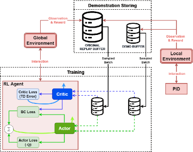
Figure 1: The flowchart of Demo-EASE based on a DDPG baseline with PID demonstration.

III-A Symmetric Local Environment

One of the main technical points of this paper is the exploitation of environment symmetry to duplicate the demonstration data and improve the training efficiency. As symmetry is conventionally task specific and noted as expert-defined in [26], we propose the following general definition for the symmetry in the environment for robot manipulation tasks.

Definition 1

For the MDP $\mathcal{M}$ defined in Section II, $\mathcal{S}_{0}\subset\mathcal{S}$ and $\mathcal{S}_{1}\subset\mathcal{S}$ are symmetric, or $\mathcal{S}_{0}\rightleftharpoons\mathcal{S}_{1}$, if there exist reversible mappings $\phi:\mathcal{S}_{1}\rightarrow\mathcal{S}_{0}$ and $\psi:\mathcal{A}\rightarrow\mathcal{A}$, such that $\phi(f(s,a))=f(\phi(s),\psi(a))$ holds for any $s\in\mathcal{S}_{1}$ and $a\in\mathcal{A}$ that satisfy $f(s,a)\in\mathcal{S}_{1}$ and $f(\phi(s),\psi(a))\in\mathcal{S}_{0}$.

Definition 1 gives a mathematical formulation of symmetry for deterministic MDP. Similar definition can also be made for stochastic MDP, which is beyond the scope of this paper. Symmetric domains that are subject to a common MDP possess the inherent homogeneity, which indicates that accurate prediction can be made on a domain given the historical observation on its symmetric counterpart even though the real observation is not available. For example, for the current state $s\in\mathcal{S}_{1}$ and action $a\in\mathcal{A}$, assume that a successive state $s^{\prime}=f(s,a)\in\mathcal{S}_{1}$ is observed. Then, it can be asserted that $\phi(s^{\prime})$ is the accurate prediction of $\phi(s)$ and $\psi(a)$ without obtaining the real observation $\phi(s^{\prime})$ for the sample $\{\phi(s),\psi(a)\}$. Note that the symmetry relation is reversible, i.e.,

$$\mathcal{S}_{0}\rightleftharpoons\mathcal{S}_{1}\Rightarrow\mathcal{S}_{1}\rightleftharpoons\mathcal{S}_{0},$$ (3)

since we know $\phi(f(s,a))=f(\phi(s),\psi(a))$ definitely lead to $f\!\left(\phi^{-1}[\phi(s)],\psi^{-1}[\psi(a)]\right)=\phi^{-1}[f(s,a)]$. Based on the definition of symmetry, we define another important concept, the symmetrically partitionable environment, as follows.

Definition 2

For the MDP $\mathcal{M}$ defined in Section II, we refer to the domain $\mathcal{S}$ as symmetrically partitionable, if $\exists\,\mathcal{S}_{0}$, $\mathcal{S}_{1}$, $\cdots$, $\mathcal{S}_{M-1}$ $\subset$ $\mathcal{S}$, where $M$ is a positive integer, such that $\mathcal{S}_{0}\cup\mathcal{S}_{1}\cup\cdots\cup\mathcal{S}_{M-1}=\mathcal{S}$, and $S_{i}\rightleftharpoons\mathcal{S}_{j}$ and $S_{i}\cap\mathcal{S}_{j}=\varnothing$ hold for all $i,j$$\,=\,$$0$, $1$, $\cdots$, $M-1$ and $i\neq j$.

Definition 2 addresses a special type of MDP, of which the state space can be split into several mutually exclusive and symmetric partitions. Such an MDP possesses a special property, i.e., for any sample $(s_{0},a_{0})\in\mathcal{S}\times\mathcal{A}$ and its observation $s^{\prime}_{0}\in\mathcal{S}$, another $M-1$ counterparts $s^{\prime}_{1}\sim(s_{1},a_{1})$, $\cdots$, $s^{\prime}_{M-1}\sim(s_{M-1},a_{M-1})$ can be generated and asserted as accurate prediction. In this paper, we refer to a symmetrically partitionable space $\mathcal{S}$ as the global environment, and any of its symmetric partitions $\mathcal{S}_{k}$, $k=0,1,\cdots,M-1$ as a local environment. In Section IV-A, we interpret how to specify local environments for a specific robot manipulation task.

III-B Demonstration

A demonstration episode is a path of the MDP $\mathcal{M}$ $\tau(\pi^{\mathrm{d}})=\left\{s_{0},a_{0},s_{1},a_{1},\cdots,s_{N_{\tau}-1},a_{N_{\tau}-1},s_{N_{\tau}}\right\}$, $N_{\tau}\in\mathbb{N}^{+}$, where $\pi^{\mathrm{d}}$ is the policy used to generate the demonstration. The demonstration policy can be generated from previous data [29], or explicit teaching [38], or an imperfect controller [39]. Demonstration contains the external information from outside the environment which may serve as prior knowledge to guide the agent through the initial learning stage. However, demonstration may be a barrier for the agent to improve its performance in the late stage of agent training, which may lead to the over-fitting problem, i.e., the agent loses the generalizability to similar tasks [40]. Therefore, a smart agent should be able to utilize the demonstration knowledge in its early learning stage, and starts to balance between the demonstration and its own experience when it becomes mature.

In this paper, we record the agent trajectories subject to a PID control as the demonstration. As a conventional and widely applied control method, PID benefits from its simplification and the excellent generalizability. For most practical applications, PID control provides decent performance, although the optimality of a specific metric is not always guaranteed. Therefore, PID control can be used as a conservative solution for general robot control and planning, although it is hard to be customized for certain tasks. For any time instant $t=0,1,\cdots,N_{\tau}$ and state $s_{t}$, a PID action $a_{t}^{\mathrm{PID}}\sim\pi^{\mathrm{d}}(s_{t})$ is defined as

$$a_{t}^{\mathrm{PID}}=K_{\mathrm{P}}\tilde{q}_{t}+K_{\mathrm{I}}\int_{0}^{t}\tilde{q}_{\tau}\mathrm{d}\tau+K_{\mathrm{D}}\dot{\tilde{q}}_{t},$$ (4)

where $\tilde{q}_{t}=q_{t}^{\mathrm{sp}}-q_{t}$, $q_{t}^{\mathrm{st}}\in\mathbb{R}^{n}$ is the desired joint angles obtained by calculating the inverse kinematics of the Cartesian set points, and $q_{t}$ is the current joint angles of the robot. For the P2P task, $q_{t}^{\mathrm{sp}}$ is the inverse kinematics of the goal position $P_{g}$. For the P2P-O task, heuristic midway points are added to $q_{t}^{\mathrm{sp}}$ such that the robot moves around the obstacle. $K_{\mathrm{P}}$, $K_{\mathrm{I}}$, and $K_{\mathrm{D}}$ are respectively the proportional gain, the integral gain, and the derivative gain of the PID controller. With the state $s_{t}$ and action $a_{t}^{\mathrm{PID}}$, the successive state $s^{\prime}_{t}$ is observed and the instant reward $r_{t}=R(s_{t},a_{t}^{\mathrm{PID}})$ is calculated. Note that all the demonstration is recorded in a local environment $\mathcal{S}_{k}$, $k=0,1,\cdots,M-1$. Each demonstration episode is terminated by a binary ending flag $\zeta_{t}\in\{0,1\}$ which is enabled when any of the following conditions hold.

1. Reaching: the reaching error $e_{t}$ is sufficiently small.

2. Timeout: $t$ exceeds the desired episode length $N_{\tau}$.

3. Collision: the state $s_{t}$ collides with the obstacle $P_{o}$.

4. The successive state $s^{\prime}_{t}$ exceeds the local environment $\mathcal{S}_{k}$.

We use $\mathcal{D}^{k}_{t}=\left\{s_{t},a^{\mathrm{PID}}_{t},s^{\prime}_{t},r_{t},\zeta_{t}\right\}$ to represent the demonstration sample at time $t$, where $k$ stands for the local environment from which the sample is obtained. Then, additional demonstration samples $\phi\!\left(\mathcal{D}_{t}^{k}\right)=\{\phi(s_{t}),a^{\mathrm{PID}},\phi(s^{\prime}_{t}),r_{t},\zeta_{t}\}$ can be duplicated on all the symmetrical local environments of $\mathcal{S}_{k}$.

III-C Demonstration Sample Storing

As shown in Fig. 1, the proposed Demo-EASE is equipped with an original replay buffer $\mathcal{B}_{\mathrm{o}}$ and a demonstration replay buffer $\mathcal{B}_{\mathrm{d}}$. $\mathcal{B}_{\mathrm{d}}$ only contains the demonstration samples $\mathcal{D}^{k}_{t}$ and their duplicates $\phi\!\left(\mathcal{D}^{k}_{t}\right)$ in all local environments, while $\mathcal{B}_{\mathrm{o}}$ contains both the demonstration samples and the normal training samples. With the sizes of $\mathcal{B}_{\mathrm{o}}$ and $\mathcal{B}_{\mathrm{d}}$ respectively denoted as $N_{\mathrm{o}}\in\mathbb{N}^{+}$ and $N_{\mathrm{d}}\in\mathbb{N}^{+}$, we assume $N_{\mathrm{d}}\ll N_{\mathrm{o}}$, such that $\mathcal{B}_{\mathrm{o}}$ has sufficient space to contain the demonstration samples in $\mathcal{B}_{\mathrm{d}}$. The storing process of the demonstration samples is described in Algorithm 1. For a symmetrically partitionable space $\mathcal{S}$ that has $M$ symmetric partitions, the demonstration samples are collected uniformly from all local environments. While we fix the initial position $q_{0}$ for each local environment, we sample the goal and obstacle positions $P_{g}$ and $P_{o}$ randomly from uniform distributions. Then, for each step $t$ of an episode, samples $\mathcal{D}_{t}^{k}$ and their duplicates $\phi\!\left(\mathcal{D}_{t}^{k}\right)$ are stored in both buffers $\mathcal{B}_{\mathrm{o}}$ and $\mathcal{B}_{\mathrm{d}}$ until the termination flag $\zeta_{t}$ is positive.

Input: Empty buffers $\mathcal{B}_{\mathrm{o}}$, $\mathcal{B}_{\mathrm{d}}$

Output: Full buffers $\mathcal{B}_{\mathrm{o}}$, $\mathcal{B}_{\mathrm{d}}$

for $i\leftarrow 1$ to $N_{\mathrm{demos}}$ do

       Uniformly sample local region $k\sim\{1,2,\cdots,M\}$

       Fix the initial robot joint angle $q_{0}$

       Uniformly sample the positions $P_{g},P_{o}\sim\mathcal{S}_{k}$

       Generate heuristic set points $q^{\mathrm{sp}}_{t}$

       $s_{t}\leftarrow q_{0}$, $t\leftarrow 0$

       while $t<N_{\tau}$ & $\zeta_{t}=0$ do

             Observe $s_{t}$ and execute $a^{\mathrm{PID}}_{t}$ from (4)

             Observe $s^{\prime}_{t}$, $r_{t}$ and determine $\zeta_{t}$

            

            Store samples $\mathcal{D}_{t}^{k},\phi\!\left(\mathcal{D}_{t}^{k}\right)\rightarrow\mathcal{B}_{\mathrm{d}},\mathcal{B}_{\mathrm{o}}$

             $s_{t}\leftarrow s_{t}^{\prime}$, $t\leftarrow t+1$

       end while

      

end for

Algorithm 1 Proposed Demonstration Storing

III-D Agent Structure and Loss functions

As shown in Fig. 1, the Demo-EASE agent has both actor and critic neural networks. We represent them as functions $\pi:\mathcal{S}\rightarrow\mathcal{A}$ and $Q:\mathcal{S}\times\mathcal{A}\rightarrow\mathbb{R}$, respectively. Similar to the conventional DDPG baseline, the Demo-EASE agent also contains two target networks $\pi^{\prime}:\mathcal{S}\rightarrow\mathcal{A}$ and $Q^{\prime}:\mathcal{S}\times\mathcal{A}\rightarrow\mathbb{R}$ which have the same structures as $\pi$ and $Q$, although they are not displayed in Fig. 1 for brevity. Note that we do not use all the samples in the replay buffers $\mathcal{B}_{\mathrm{o}}$ and $\mathcal{B}_{\mathrm{d}}$ to update the networks for limiting the computational load. Instead, we use two smaller batch buffers $\overline{\mathcal{B}}_{\mathrm{o}}$ and $\overline{\mathcal{B}}_{\mathrm{d}}$ which contain the shuffled and sampled samples of $\mathcal{B}_{\mathrm{o}}$ and $\mathcal{B}_{\mathrm{d}}$, respectively. The sizes of $\overline{\mathcal{B}}_{\mathrm{o}}$ and $\overline{\mathcal{B}}_{\mathrm{d}}$ are respectively $\overline{N}_{\mathrm{o}}$ and $\overline{N}_{\mathrm{d}}$ which satisfy $\overline{N}_{\mathrm{d}}<N_{\mathrm{d}}$ and $\overline{N}_{\mathrm{o}}<N_{\mathrm{o}}$. Then, the conventional critic loss function used to update the critic networks $Q$ and $Q^{\prime}$ reads

$$\begin{split}\mathcal{L}_{C}\!\left(\overline{\mathcal{B}}_{\mathrm{o}}\right)=\frac{1}{\overline{N}_{\mathrm{o}}}\sum_{t=0}^{\overline{N}_{\mathrm{o}}-1}&\left(r_{t}-Q(s_{t},\pi(s_{t}))\right.\\ &+\left.\gamma(1-\zeta_{t})Q^{\prime}(s^{\prime}_{t},\pi^{\prime}(s^{\prime}_{t}))\right)^{2},\end{split}$$ (5)

where $\{s_{t},a_{t},r_{t},s^{\prime}_{t},\zeta_{t}\}\sim\overline{\mathcal{B}}_{\mathrm{o}}$. The actor networks $\pi,\pi^{\prime}$ are updated using both batch buffers $\overline{\mathcal{B}}_{\mathrm{o}}$ and $\overline{\mathcal{B}}_{\mathrm{d}}$ with a combined loss function

$$\mathcal{L}_{A}\!\left(\overline{\mathcal{B}}_{\mathrm{o}},\overline{\mathcal{B}}_{\mathrm{d}}\right)=\mathcal{L}_{O}\!\left(\overline{\mathcal{B}}_{\mathrm{o}}\right)+\lambda_{BC}\mathcal{L}_{BC}\!\left(\overline{\mathcal{B}}_{\mathrm{d}}\right),$$ (6)

where $\mathcal{L}_{O}$ is the original actor loss function defined as:

$$\mathcal{L}_{O}\!\left(\overline{\mathcal{B}}_{\mathrm{o}}\right)=-\frac{1}{\overline{N}_{\mathrm{o}}}\sum_{t=0}^{\overline{N}_{\mathrm{o}}-1}Q(s_{t},\pi(s_{t})),$$ (7)

$\mathcal{L}_{BC}$ is a behavior cloning loss function used to enable the compatibility between the two buffers, and $\lambda_{BC}$ is a hyper-parameter to adjust the proportion of behavior cloning. The behavior cloning loss function $\mathcal{L}_{BC}$, inspired by the behavior cloning in imitation learning [29], is defined as

$$\mathcal{L}_{BC}\!\left(\overline{\mathcal{B}}_{\mathrm{d}}\right)=\frac{1}{\overline{N}_{\mathrm{d}}}\sum_{t=0}^{\overline{N}_{\mathrm{d}}-1}M_{t}\left(a_{t}^{\mathrm{d}}-\hat{a}_{t}\right)^{2},$$ (8)

where $\hat{a}_{t}=\pi\!\left(s_{t}^{\mathrm{d}}\right)$ is the agent action subject to the current policy $\pi$ and the demonstration state $s^{\mathrm{d}}_{t}$, $\left(s_{t}^{\mathrm{d}},a_{t}^{\mathrm{d}}\right)\sim\overline{\mathcal{B}}_{\mathrm{d}}$, and $M_{t}$ is a binary mask that indicates whether the demonstration action $a^{\mathrm{d}}_{t}$ is superior than the current policy action $a_{t}$, i.e.,

$$M_{t}=\left\{\begin{array}[]{ll}1,&\text{if}\ Q(s_{t}^{\mathrm{d}},\hat{a}_{t})<Q(s_{t}^{\mathrm{d}},a^{\mathrm{d}}_{t})\\ 0,&\text{otherwise}.\end{array}\right.$$ (9)

The purpose of the actor loss function $\mathcal{L}_{\mathcal{BC}}$ is to balance between the knowledge contained in the demonstration and the own experience of the agent by comparing the values of the corresponding actions. In the initial state of the training, when the current policy $\pi$ is of low quality, $\pi$ imitates the demonstration policy $\pi^{\mathrm{d}}$, which is referred to as behavior cloning. When the agent is well trained such that its own policy $\pi$ is superior than the demonstration, $\mathcal{L}_{BC}$ vanishes and the demonstration policy $\pi^{\mathrm{d}}$ is ignored. A hyper-parameter $\lambda_{BC}$, referred to as the behavior cloning gain, is involved to adjust the extent of cloning and avoid absolute imitation of the demonstration. In this sense, the demonstration guides the agent to grow when it is young, but encourage the agent to follow its own policy when it becomes mature. In such a manner, Demo-EASE can achieve the balance between the training efficiency and the generalizability of the agent. The cloning gain $\lambda_{BC}$ and the number of demonstration samples $N_{\mathrm{demos}}$ are the two important hyper-parameters using which we control the involvement of demonstration to the agent training.

III-E Training of A Demo-EASE Agent

The overall training algorithm of the Demo-EASE agent based on a DDPG baseline is presented in Algorithm 2, which is partially inspired by our previous work [26]. Different from the previous work which uses a well trained DDPG agent to generate the demonstration, we focus on the knowledge transference from a readily developed but a non-optimal controller to showcase the capability of our method in leveraging the existing controllers on improving their performance. It is also the first time that symmetric demonstration is applied to robot manipulation tasks. DDPG is selected due to its capability of randomly exploring the environment and its compatibility with continuous action spaces, although the proposed framework is promising to be extended to all off-policy methods that are equipped with experience replay. Different from the conventional DDPG baseline, Algorithm 2 uses batch buffers $\overline{\mathcal{B}}_{\mathrm{o}}$ and $\overline{\mathcal{B}}_{\mathrm{d}}$ to update the neural networks $\pi_{\mu}$ and $Q_{\nu}$. Also, the actor loss function $\mathcal{L}_{A}$ contains an additional loss function $\mathcal{L}_{BC}$ which controls the learning from the demonstration. In algorithm 2, $N_{\mathrm{eq}}\in\mathbb{N}^{+}$ is the number of episodes, $N_{\mathrm{up}}\in\mathbb{N}^{+}$ is the number of epochs after which the networks are updated, $N_{\tau}\in\mathbb{N}^{+}$ is the maximum length of each episode, $\sigma\in\mathbb{R}^{+}$ is the standard deviation of the action exploration, and $\omega\in\mathbb{R}^{+}$ is the coefficient of target network updates.

Input: parameters $\mu$, $\nu$ for initial policy $\pi_{\mu}$, value $Q_{\nu}$,

parameters $\mu^{\prime}\!\leftarrow\!\mu$, $\nu^{\prime}\!\leftarrow\!\nu$ for target networks $\pi^{\prime}_{\mu^{\prime}}$, $Q^{\prime}_{\nu^{\prime}}$,

and full replay buffers $\mathcal{B}_{\mathrm{o}}$, $\mathcal{B}_{\mathrm{d}}$ from Algorithm 1.

Output: trained policy $\pi_{\mu}$ and value $Q_{\nu}$.

for $i\leftarrow 1$ to $N_{\mathrm{ep}}$ do

      

      for $j\leftarrow 0$ to $N_{\mathrm{up}}$ do

            

            $s_{t}\leftarrow q_{0}$, $t\leftarrow 0$

             while $t<N_{\tau}$ & $\zeta_{t}=0$ do

                   Observe $s_{t}$ and execute $a_{t}\sim\mathcal{N}\!\left(\pi_{\theta}(s_{t}),\sigma\right)$

                   Observe $s^{\prime}_{t}$, $r_{t}$ and determine $\zeta_{t}$

                   Store sample $\left\{s_{t},a_{t},r_{t},s^{\prime}_{t},\zeta_{t}\right\}\rightarrow\mathcal{B}_{\mathrm{o}}$

                   $s_{t}\leftarrow s_{t}^{\prime}$, $t\leftarrow t+1$

             end while

            

       end for

      

      Sample batch buffers $\overline{\mathcal{B}}_{\mathrm{o}}\sim\mathcal{B}_{\mathrm{o}}$, $\overline{\mathcal{B}}_{\mathrm{d}}\sim\mathcal{B}_{\mathrm{d}}$

       Calculate $\mathcal{L}_{C}$ using (5) and $\nabla_{\nu}\mathcal{L}_{C}$

       Calculate $\mathcal{L}_{O}$ and $\mathcal{L}_{BC}$ using (7) and (8)

       Calculate $\mathcal{L}_{A}$ using (6) and $\nabla_{\mu}\mathcal{L}_{A}$

       Update networks $\pi_{\mu},Q_{\nu}$ by gradient descent

       $\mu\leftarrow\mu+\alpha_{\mu}\nabla_{\mu}\mathcal{L}_{A}$ , $\nu\leftarrow\nu+\alpha_{\nu}\nabla_{\nu}\mathcal{L}_{C}$

       Update the target networks $\pi^{\prime}_{\mu^{\prime}},Q^{\prime}_{\nu^{\prime}}$ by

       $\mu^{\prime}\leftarrow\omega\mu^{\prime}+(1-\omega)\mu,\ \nu^{\prime}\leftarrow\omega\nu^{\prime}+(1-\omega)\nu$

end for

Algorithm 2 Demo-EASE Training based on DDPG

IV Experimental Setup

To validate the proposed method, we setup a simulation experiment in the PyBullet environment using a 6-DoF Kinova® Gen3 robot model with a Robotiq® 2F-85 gripper as shown in Fig. 2. Since our experiments do not involve complex dexterity, only four actuators (# 1, # 2, # 3, and # 4) are active and the other two are locked, as shown in Fig. 2, which leads to a 4-DoF robot model. The experimental simulation is performed on a computer workstation equipped with an AMD Ryzen 9 5900X CPU, an Nvidia RTX 3090 GPU, and 64GB (2x32) Corsair DDR4 memory, with Ubuntu 18.04.6 LTS operating system. We use spinningup [41] as the DDPG benchmark to develop our method. The configuration of the P2P and the P2P-O tasks are interpreted as follows.

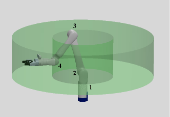
Figure 2: The 6-DoF Kinova® Gen3 robot model. The workspace is the green tube showing $min$ and $max$ extremities of polar radius and height. The four active joints are labeled as well.

IV-A Environment Partition

Fig. 3 shows the top-to-bottom view of the workspace where the base of the robot is placed in the geometry center of the workspace. We split the entire workspace $\mathcal{S}$ into four partitions, $\mathcal{S}_{0}$, $\mathcal{S}_{1}$, $\mathcal{S}_{2}$, and $\mathcal{S}_{3}$, as shown in Fig. 3. The partitions can be represented by the following polar coordinates.

$$\mathcal{S}_{0}= \,\left\{(\theta,\rho,z)\left|0\leq\theta<\frac{\pi}{2},\,\rho\leq\xi(\theta),\,z>0\right.\right\},$$

$$\mathcal{S}_{1}= \,\left\{(\theta,\rho,z)\left|\frac{\pi}{2}\leq\theta<\pi,\,\rho\leq\xi\!\left(\theta-\frac{\pi}{2}\right),\,z>0\right.\right\},$$

$$\mathcal{S}_{2}= \,\left\{(\theta,\rho,z)\left|\pi\leq\theta<\frac{3\pi}{2},\,\rho\leq\xi(\theta-\pi),\,z>0\right.\right\},$$

$$\mathcal{S}_{3}= \,\left\{(\theta,\rho,z)\left|\frac{3\pi}{2}\leq\theta<2\pi,\,\rho\leq\xi\!\left(\theta-\frac{3\pi}{2}\right),\,z>0\right.\right\},$$

where $\theta,r,z\in\mathbb{R}$ are respectively the rotation angle, radius, and height of the polar coordinate, and $\xi(\theta)$ is the safety boundary of the environment. In the case of box-shape boundary as shown in Fig. 3,

$$\xi(\theta)=\left\{\begin{array}[]{ll}\tan(\theta),&\displaystyle 0\leq\theta<\frac{\pi}{4},\\ \displaystyle\tan\left(\frac{\pi}{2}-\theta\right),&\displaystyle\frac{\pi}{4}\leq\theta<\frac{\pi}{2}.\end{array}\right.$$ (10)

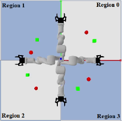
Figure 3: Division of the workspace into four symmetric partitions as local environments for generating demonstrations.

Now, we justify the symmetry among the four partitions. Without losing generality, we take $\mathcal{S}_{0}$ and $\mathcal{S}_{1}$ as an example. Subject to the same control policy, it is straightforward that the resulting robot trajectories also have the same shape, other than that they are relatively rotated to the base of the robot, as shown in Fig. 3. In fact, for any robot state $s\in\mathcal{S}_{0}$ and action $a\in\mathcal{A}$ such that the successive state $s^{\prime}\in\mathcal{S}_{0}$, there always exist two invertable mappings $\phi:\mathcal{S}_{0}\rightarrow\mathcal{S}_{1}$ and $\psi:\mathcal{A}\rightarrow\mathcal{A}$, where $\psi(a)=a$ and

$$\phi(s_{t})=\left[\,q_{t}^{\phi},\,\sin(q_{t}^{\phi}),\,\cos(q_{t}^{\phi}),\,\dot{q}_{t},\,P_{g},\,e_{t}^{\phi}\,\right],$$ (11)

where $q_{t}^{\phi}$ adds ${\pi}/{2}$ to the robot base joint angle compared to $q_{t}$, such that $\phi(s)\in\mathcal{S}_{1}$ and $\phi(s)^{\prime}=\phi(s^{\prime})\in\mathcal{S}_{1}$, and $e_{t}^{\phi}=P_{g}-(P_{t}^{e})^{\phi}$ is the reaching error, where $(P_{t}^{e})^{\phi}$ is the transformed end-effector position from $P_{t}^{e}$ with rotation angle $\pi/2$ related to the origin. Thus, according to Definition 1, we know that $\mathcal{S}_{0}$ and $\mathcal{S}_{1}$ are symmetric. Such a property can easily be verified for other partitions, which leads to that the four partitions are symmetric to each other. According to Definition 2, the workspace $\mathcal{S}$ is symmetrically partitionable. The workspace being symmetrically partitionable means that, for any sample $\mathcal{D}_{t}$ collected on $\mathcal{S}\times\mathcal{A}$, another $M-1$ samples can be duplicated without real demonstrations.

IV-B Demonstration Storing

For each episode of both the P2P and the P2P-O tasks, the robot moves from an initial joint angle $q_{0}\in\mathbb{R}^{n}$ to reach the goal position $P_{g}\in\mathbb{R}^{3}$. For different stages, demonstration recording, training, and test, the initial joint angle $q_{0}$ and the goal position $P_{g}$ are sampled differently to evaluate the generalizability of the agent. The P2P-O task also involves the sampling of the obstacle position $P_{o}$ which is sampled according to the robot configuration. The demonstration is recorded in local environments $\mathcal{S}_{k}$, where $k\sim\left\{1,2,3,4\right\}$ is uniformly sampled, while the training and test are performed in the global environment $\mathcal{S}$.

IV-B1 Configuration of the P2P task

For the P2P task, we sample the initial end-effector position as

$$\theta_{0}\sim\left\{\frac{k\pi}{2}-\frac{\pi}{4}\right\},~{}\rho_{0}=0.52,~{}z_{0}=0.42,$$

for all $k\sim\left\{0,1,2,3\right\}$. Here, we use the polar coordinate $(\theta_{0},\rho_{0},z_{0})$ to represent the end-effector position in the workspace. Then, inverse kinematics is calculated to obtain the initial joint angles $q_{0}$. The goal position $(\theta_{g},\rho_{g},z_{g})$ is uniformly sampled from

$$\theta_{g}\sim\left[\frac{k\pi}{2}-\frac{\pi}{2},\frac{k\pi}{2}\right),\ \rho_{g}\sim[\,0.4,\,0.6\,),\ z_{g}\sim[\,0.35,\,0.55\,),$$

which is then transformed to the Cartesian coordinate $P_{g}$. In such a manner, the sampled goal is restricted to the same local environment as the initial position of the robot end-effector. The number of the demonstration episodes $N_{\mathrm{demos}}$ is selected as 0, 80, and 160 for the comparison study. Four examples of P2P demonstrations are illustrated in Fig. 4(a).

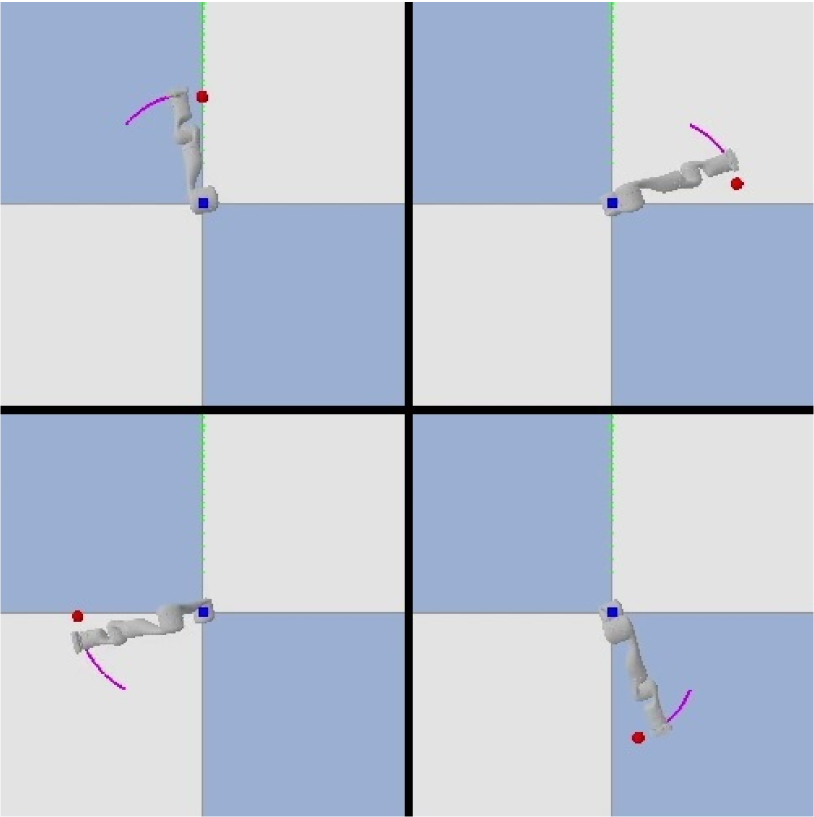
(a) P2P

(b) P2P with obstacle

Figure 4: Examples of the abstract demonstrations used to prepare the local demonstration replay buffers

IV-B2 Configuration of the P2P-O)

For the P2P-O task, the initial position of the robot end-effector is uniformly sampled from

$$\theta_{0}\sim\left\{\frac{k\pi}{2}\right\},~{}\rho_{0}=0.52,~{}z_{0}=0.42,$$

for all $k\sim\{0,1,2,3\}$, which is then transformed to the initial joint angle $q_{0}$. The target position $P_{g}$ is sampled from

$$\theta_{g}\sim\left[\frac{k\pi}{2}-\frac{\pi}{4},\frac{k\pi}{2}\right),\ \rho_{g}\sim[\,0.4,\,0.6\,),\ z_{g}\sim[\,0.35,\,0.55\,).$$

A cubic obstacle sized $0.04\,$m is placed at position $P_{o}$ which is determined base on the goal position so that it is located between the initial position of the gripper and the target,

$$\theta_{o}\sim\left[\theta_{g}-\frac{k\pi}{6},\theta_{g}-\frac{k\pi}{12}\right),\ z_{o}\sim[\,z_{g}-0.1,z_{g}+0.1\,).$$ (12)

The subscript $o$ indicates the coordinate of the obstacle. The number of demonstration episodes $N_{\mathrm{demos}}$ is set as 100, 200, and 400 for the comparison study. It is in general larger than that in the P2P task due to the complexity of P2P-O.

IV-C Agent Training

The training of the agent is performed in the global environment $\mathcal{S}$. For both the P2P and the P2P-O tasks, the initial position of the robot end-effector is fixed in

$$\theta_{0}=\pi/4,~{}\rho_{0}=0.52,~{}z_{0}=0.42,$$ (13)

and the target positions= $P_{g}$ is sampled from

$$\theta_{g}\sim[\,-\pi,\,\pi\,),\ \rho_{g}\sim[\,0.3,\,0.7\,),\ z_{g}\sim[\,0.25,\,0.65\,).$$ (14)

For the P2P-O task, the obstacle position is sampled from

$$\begin{split}\theta_{b}=\theta_{g}+\mathrm{sgn}(\theta_{1}-0.5)\theta_{2},\\ \rho_{b}\sim[\,0.4,\,0.6\,),\\ z_{b}\sim[z_{g}-0.1,z_{g}+0.1),\end{split}$$ (15)

where $\mathrm{sgn}(\cdot)$ is the sign function that produces $1$, $-1$, and $0$ for positive, negative, and zero values, respectively. $\theta_{1}\sim[\,0,~{}1\,)$ and $\theta_{2}\sim\left[\,{k\pi}/{12},{k\pi}/{6}\,\right)$ are random variables sampled from uniform distributions. Such a definition of $\theta_{b}$ is to ensure that the block is forced to be towards clockwise or counter clockwise direction from the target in the global space.

The reward function $R$ for both tasks is selected based on the following concerns.

1. Approaching: Penalize the reaching error at each time.

2. Effort: Encourage the agent to consume minimum effort.

3. Reaching: Encourage ultimately reaching the goal.

4. Collision: Penalize any collisions with the obstacle.

Thus, we design the following reward function,

$$R(s_{t},a_{t})=r^{\mathrm{dst}}_{t}+r^{\mathrm{eft}}_{t}+r^{\mathrm{rch}}_{t}+r^{\mathrm{cls}}_{t}.$$ (16)

The first term $r^{\mathrm{dst}}_{t}$ is to penalize the reaching error $e_{t}$,

$$r^{\mathrm{dst}}_{t}=-\alpha_{1}||e_{t}||,$$ (17)

where $\alpha_{1}\in\mathbb{R}^{+}$ is hyper-parameter to be determined. This term stimulates the reaching towards the goal. The second term $r^{\mathrm{eft}}_{t}$ is to penalize the actuation torques of the robot,

$$r^{\mathrm{eft}}_{t}=-\alpha_{2}\left\|\hat{\tau}_{t}\right\|,$$ (18)

where $\alpha_{2}$ is a parameter and $\hat{\tau}_{t}=\left[\,\hat{\tau}_{t}^{(1)}~{}\hat{\tau}_{t}^{(2)}~{}\hat{\tau}_{t}^{(3)}~{}\hat{\tau}_{t}^{(4)}\,\right]^{\top}$ are the normalized actuation torques of the four active joints of the robot. For each joint $j$, $\hat{\tau}_{t}^{(j)}=\left|\tau_{t}^{(j)}\right|/\tau^{(j)}_{\max}$, where $\tau_{t}^{(j)}$ is the actual actuation torque at time $t$ and $\tau^{(j)}_{\max}$ is the maximum torque, where $\tau^{(1,2,3)}_{\max}=39\,$N$\cdot$m and $\tau^{(4)}_{\max}=9\,$N$\cdot$m. The third term $r^{\mathrm{rch}}_{t}$ gives a big positive reward for ultimately reaching the goal,

$$r^{\mathrm{rch}}_{t}=\left\{\begin{array}[]{ll}0,&\text{if}\left\|e_{t}\right\|\geq\varepsilon\\ R_{1},&\text{else},\end{array}\right.$$ (19)

where $\varepsilon=0.05\,$m is the tolerated reaching error, and the last term $r^{\mathrm{cls}}_{t}$ exerts a big negative reward for collision either with the obstacle or the robot itself,

$$r^{\mathrm{cls}}_{t}=\left\{\begin{array}[]{ll}-R_{2},&\text{if collision detected}\\ 0,&\text{else}\end{array}\right.$$ (20)

where $\varepsilon,R_{1},R_{2}\in\mathbb{R}^{+}$ are parameters. For the reward function, the parameters are selected as $\alpha_{1}=2\times 10^{-3}$, $\alpha_{2}=10^{-3}$, $R_{1}=10$, and $R_{2}=2$.

The structure of the neural networks $\pi_{\mu}$, $\pi^{\prime}_{\mu^{\prime}}$, $Q_{\nu}$, $Q^{\prime}_{\nu^{\prime}}$ is selected as $[\,128,~{}512,~{}128\,]$ and $[\,256,~{}1024,~{}256\,]$, respectively. The behavior cloning gain $\lambda_{BC}$ is determined as $\{\,0.1,~{}0.6,~{}1.8\,\}$ and $\{\,100,~{}200,~{}400\,\}$, respectively, for the purpose of comparison study. The remaining parameters of the agent training are indicated in Tab. I.

TABLE I: The Value of the Training Parameters

Parameter	Name	P2P	P2P-O
$N_{\tau}$	Max Episode Length	400	500
$N_{\mathrm{ep}}$	Number of epochs	250	500
$N_{\mathrm{o}}$	Size of $\mathcal{B}_{\mathrm{o}}$	$10^{6}$
$\overline{N}_{\mathrm{o}}$	Size of $\overline{\mathcal{B}}_{\mathrm{o}}$	100
$\overline{N}_{\mathrm{d}}$	Size of $\overline{\mathcal{B}}_{\mathrm{d}}$	100
$N_{\mathrm{up}}$	Update interval	20	25
$\sigma$	Exploration Noise Std. Dev.	$0.1$
$\omega$	Target update coefficient	$0.995$
$\alpha_{\mu},\ \alpha_{\nu}$	Agent’s learning rates	$10^{-3}$

V Results

In this section, we analyze the results obtained from Section IV and evaluate the performance of the proposed method.

V-A The Training Results

To evaluate the influence of different configurations of the method on the performance, we focus on two important hyper-parameters, namely the number of demonstrations $\overline{N}_{\mathrm{d}}$, and the behavior cloning gain $\lambda_{BC}$. For each combination of $N_{\mathrm{demos}}$ and $\lambda_{BC}$, five repeats are performed to reduce the effect of randomization. A conventional DDPG agent is also trained for comparison, corresponding to $N_{\mathrm{demos}}=0$ and $\lambda=0$. In this paper, we mainly use the learning curves, i.e., the change of accumulated reward over time, to evaluate the training performance. Besides, we also propose the following numerical metrics.

• Initial reward $\overline{R}_{10}$: the averaged accumulated reward over the initial 10% episode steps (0 - $10\%$), which represents the performance of the initial policies;

• Ultimate reward $\overline{R}_{90}$: the averaged accumulated reward over the ultimate 10% episode steps (90% to 100%), which depicts the performance of the trained policies;

• Reward Increment $I_{R}=\overline{R}_{90}-\overline{R}_{10}$: the increase of the accumulated reward during training;

• Half-trained time $T_{50}$: the percentage of the episode at which the accumulated reward first exceed 50% of $\overline{R}_{90}$, used to depict whether the agent is well trained.

V-A1 The Training Performance of the P2P Task

The learning curves of the P2P task during the agent training stage is presented in Fig. 5. Specifically, the results depicting the influence of the number of demonstrations $N_{\mathrm{demos}}$ and the behavior cloning gain $\lambda_{BC}$ are respectively illustrated in Fig. 5(a) and Fig. 5(b). From Fig. 5(a), it can be noticed that agents trained using demonstration show significant advantage over the original DDGP baseline. As expected, the original DDPG spends a long time to slightly increase, while the accumulated reward remains in a low level. On the contrary, the learning curves of all Demo-EASE agent start the obvious growth after around 200 episodes. After 1000 episodes, the Demo-EASE agents become mature and reach their performance ceilings. A general trend can be witnessed that the more demonstration involved in training, the higher the accumulated reward tends to be during the training process. Thus, we can infer that the exploitation of demonstration is positive to the training performance of the agent.

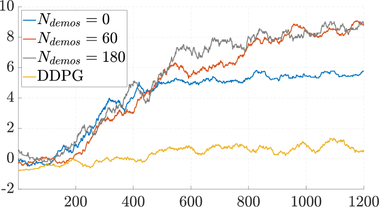
(a) Effect of different numbers of demos $N_{\mathrm{demos}}$.

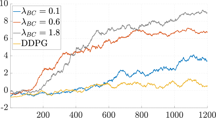
(b) Effect of different behavior cloning gains $\lambda_{BC}$.

Figure 5: The P2P learning curves of various hyper-parameters

Fig. 5(b) also shows that the Demo-EASE agents with different $\lambda_{BC}$ values present superior training performance than the original DDPG baseline. Besides, larger $\lambda_{BC}$ tends to lead to higher rewards. The agent with the smallest $\lambda_{BC}$ shows similar slow increase in the initial stage to the DDPG, but later achieves high training performance. The agents with high $\lambda_{BC}$, however, present fast increase in the very early stage (around 200 episodes), and remain a steady performance after 1000 episodes. Therefore, the results show that $\lambda_{BC}$ also play a positive role in the training process. More quantized evaluation results are revealed by the numerical metrics listed in Tab. II. The results clearly show that agents with largest $\lambda_{BC}$ and $N_{\mathrm{demos}}$ have the highest reward increment. Also, the $T_{50}$ shows that the Demo-EASE agent achieves high rewards in very early stage of training.

TABLE II: Numerical Metrics for the training of P2P

Agent	$\lambda_{BC}$, ($N_{\mathrm{demos}}=100$)			$N_{\mathrm{demos}}$, $(\lambda_{BC}=1$)			DDPG
	0.1	0.6	1.8	0	80	160
$\overline{R}_{10}$	-0.44	-0.06	-0.12	-0.28	-0.13	0.06	-0.56
$\overline{R}_{90}$	1.81	5.36	5.95	3.79	4.57	5.11	0.32
$I_{R}$	2.25	5.42	6.07	4.07	4.70	5.05	0.88
$T_{50}$	1115	574	485	296	491	486	487

V-A2 The Training of P2P-O Task

The learning curves of the P2P-O task during the agent training stage is shown in Fig. 6. Specifically, the results showing the influence of the number of demonstrations $N_{\mathrm{demos}}$ and the behavior cloning gain $\lambda_{BC}$ are respectively illustrated in Fig. 6(a) and Fig. 6(b). From both figures, it can be seen that all curves take longer time to converge than the P2P task. This is because P2P-O task is more complicated than P2P due to the augmented state space to incorporate the obstacle positions. As a result, the DDPG agent hardly have any performance promotion since 2500 episodes are too short for it to learn. On the contrary, all Demo-EASE agents show fast convergence and high rewards. In general, we can notice a general trend that larger $N_{\mathrm{demos}}$ and $\lambda_{BC}$ lead to faster convergence and higher reward, which is similar to the P2P task, although the trend is not as obvious as possible. This is probably because that the agents are not yet well trained after 2500 episodes, which is understandable considering the complexity of the P2P-O task. The numerical metrics of the P2P-O task is shown in Tab. III. Similar to Tab. II, we also notice that the agents with the largest $N_{\mathrm{demos}}$ and $\lambda_{BC}$ have the highest reward increase. Large $T_{50}$ values indicate that the curves will continue to increase after 2500 episodes. Thus, the results show that higher values of $N_{\mathrm{demos}}$ and $\lambda_{BC}$ can improve the training performance for both P2P and P2P-O tasks.

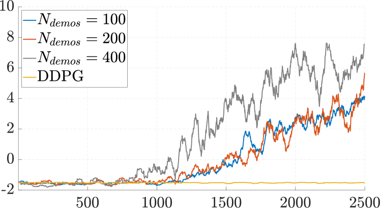
(a) Effect of different numbers of demos

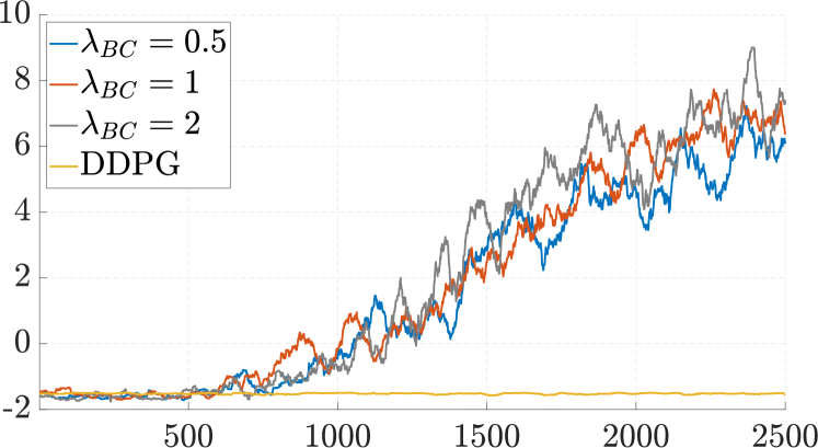
(b) Effect of different behavior cloning gains

Figure 6: The P2P-O learning curves of various hyper-parameters.

TABLE III: Numerical Metrics for the training of P2P-O

Agent	$\lambda_{BC}$, ($N_{\mathrm{demos}}=250$)			$N_{\mathrm{demos}}$, ($\lambda_{BC}=1$)			DDPG
	0.5	1	2	100	200	400
$\overline{R}_{10}$	-1.61	-1.51	-1.62	-1.53	-1.51	-1.67	-1.51
$\overline{R}_{90}$	1.01	1.27	1.47	-0.37	-0.37	1.25	-1.52
$I_{R}$	2.62	2.78	3.09	1.16	1.14	2.92	-0.01
$T_{50}$	1552	1694	1626	1639	1995	1491	50

V-B The Test Study

In this section, we deploy the trained agents onto the robot simulation model and evaluates their test performance. The test study is also conducted in the global environment, with 500 trials each task. The initial robot end-effector position is fixed as $\theta_{0}=-{\pi}/{4}$, $\rho_{0}=0.5$, $z_{0}=0.45$ for P2P and $\theta_{0}=-{\pi}/{2}$, $\rho_{0}=0.5$, $z_{0}=0.45$ for P2P-O. The robot goal configuration is sampled from the same distribution as (14). Each test trial ends if the Reaching, Timeout, and Collision criteria in Section III-B are met. Besides, we refer to the trajectories that meet the Reaching criterion as successful trials. Examples of the successful trials in the simulation environment of the test study are illustrated in Fig. 7.

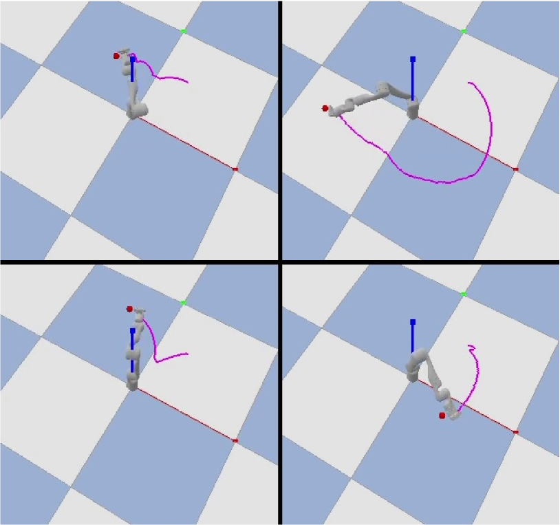
(a) P2P

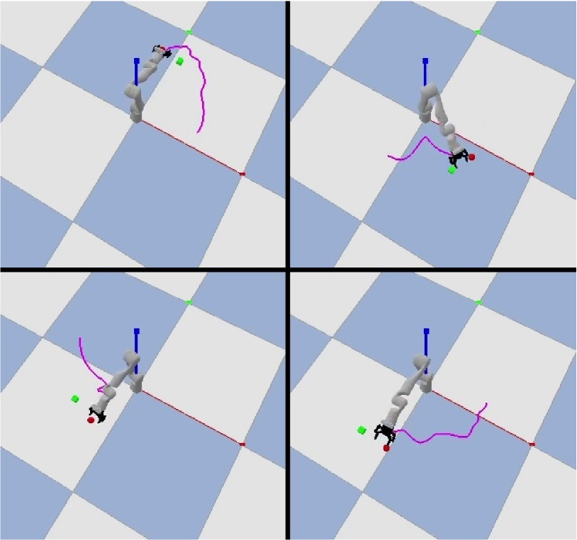
(b) P2P with obstacle

Figure 7: Samples of successful trials of trained agents

The reaching error trajectories $\|e_{t}\|$ of the P2P and P2P-O tasks in the test study, subject to different values of $\lambda_{BC}$ and $N_{\mathrm{demos}}$, are respectively illustrated in Fig. 8 and Fig. 9. In both figures, the dark curve represents the averaged trajectory over all successful trials without any collisions, while the shadow region denotes the standard variation of the trajectories. As shown in the figures, the average error decreases as time increases, which indicates that the trained Demo-EASE agent is able to execute the reaching task in general. The best results are respectively $\lambda_{BC}=1.8$ and $N_{\mathrm{demos}}=100$ for P2P and $\lambda_{BC}=2$ and $N_{\mathrm{demos}}=250$ for P2P-O, which show the smoothness and decreasing variation of the trajectories. Therefore, we can conclude that the behavior cloning and demonstration contribute to generating smooth and stable trajectories in test.

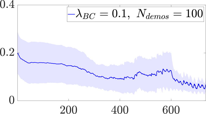
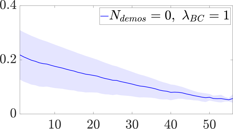
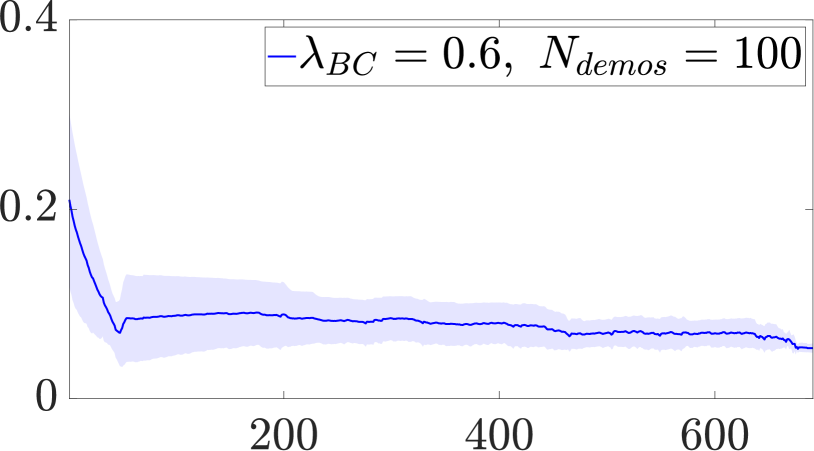
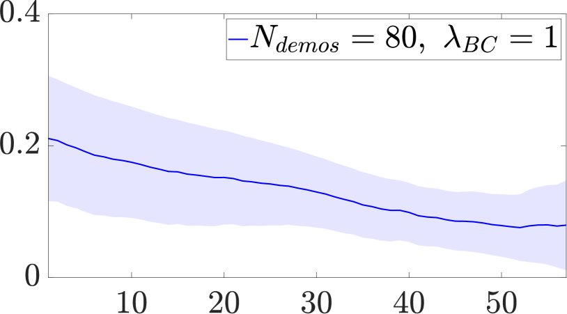
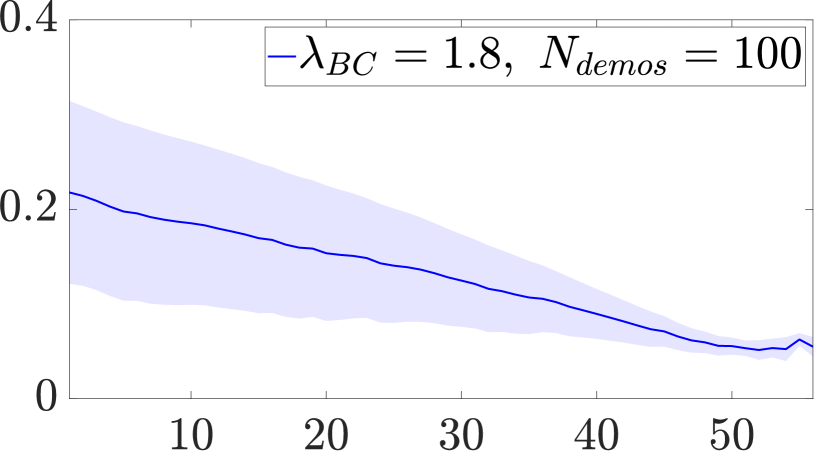
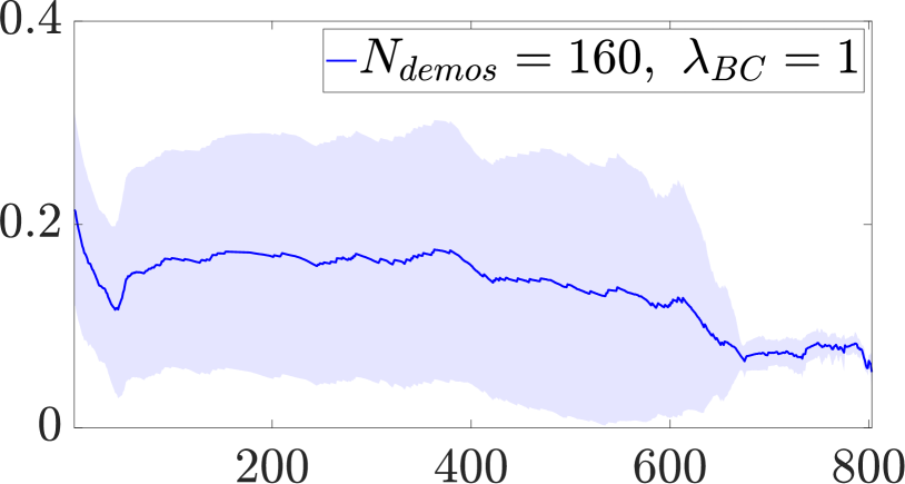
Figure 8: The average error $\|e_{t}\|$ and its standard deviation in successful trials over time $t$ in the P2P test.

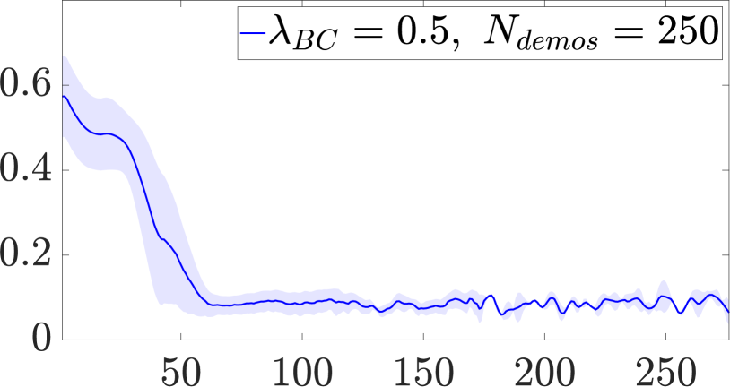
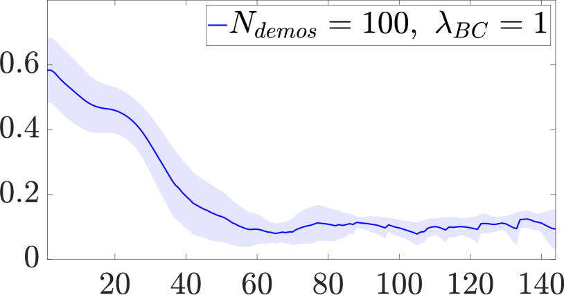
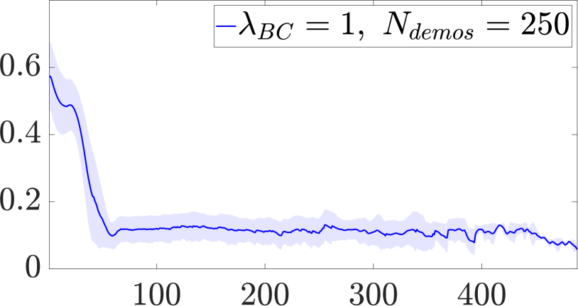
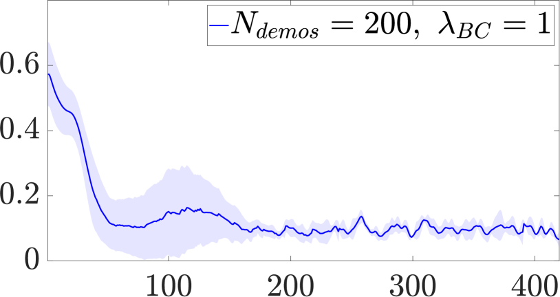
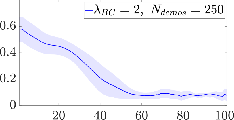
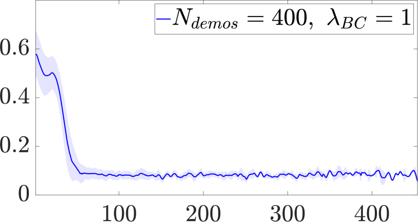
Figure 9: The average error $\|e_{t}\|$ and its standard deviation in successful trials over time $t$ in the P2P-O test.

In the test study, we also use the following metrics to evaluate the performance of the trained agent.

• Successful rate $P_{\mathrm{scs}}$: the percentage of successful trials over all trials, defined as

  $$P_{\mathrm{scs}}=\frac{N_{\mathrm{scs}}}{N_{\mathrm{ttl}}},$$ (21)

  where $N_{\mathrm{scs}},N_{\mathrm{ttl}}\in\mathbb{N}+$ are respectively the numbers of successful trials and all trials.

• Average effort $\overline{T}_{\mathrm{eff}}$: used to evaluate how much robot actuation effort is applied. For this, a similar definition of overall torque utility as in Section IV-C is used in each timestep. We average it then over all the timesteps in all of the trials as in the following equation.

  $$\overline{T}_{\mathrm{eff}}=\frac{1}{N_{\mathrm{ttl}}}\frac{1}{N_{\tau}}\sum_{i=1}^{N_{\mathrm{ttl}}}\sum_{t=1}^{N_{\tau}}\left\|\hat{\tau}_{t}^{i}\right\|.$$ (22)

  where the superscript $i$ denotes the $i$-th trial.

• Average test reward $\overline{R}_{\mathrm{test}}$: the averaged test accumulated reward over all test trials,

  $$\overline{R}_{\mathrm{test}}=\frac{1}{N_{\mathrm{scs}}}\sum_{i=1}^{N_{\mathrm{scs}}}\sum_{t=0}^{N_{\tau}}R(s^{i}_{t},a^{i}_{t})$$ (23)

  where the superscript $i$ denotes the $i$-th trial.

• Ultimate error $\overline{E}_{\overline{95}}$: the averaged ultimate obstacle reaching error over the final 5% of a successful trial,

  $$\overline{E}_{\overline{95}}=\frac{1}{N_{\mathrm{scs}}}\frac{1}{0.05N_{\tau}}\sum_{j=1}^{N_{\mathrm{scs}}}\sum_{t=0.95N_{\tau}}^{N_{\tau}}\left\|e_{t}^{(j)}\right\|,$$ (24)

  where $e_{t}^{(j)}$ is the reaching error of trial $j$ at time $t$.

The numerical metrics of both the P2P and P2P-O agents in the test study, subject to different hyper-parameters $N_{\mathrm{demos}}$ and $\lambda_{BC}$, are respectively presented in Tab. IV and Tab. V. A PID controller designed as (4) is also tested for comparison. Both tables indicate that the PID baseline shows mediocre success rate ($P_{\mathrm{\mathrm{scs}}}$) and ultimate error ($\overline{E}_{\overline{95}}$) compared to the Demo-EASE agents. Meanwhile, PID also has the lowest average effort ($\overline{T}_{\mathrm{eff}}$) and the lowest average reward ($\overline{R}_{\mathrm{test}}$). This confirms that PID is a conservative control baseline which produces smooth and energy-saving trajectories but neglect the optimality of specific tasks. For the Demo-EASE agents, larger $\lambda_{BC}$ and $N_{\mathrm{demos}}$ lead to better performance, in terms of higher success rate ($P_{\mathrm{\mathrm{scs}}}$), lower effort consumption ($\overline{T}_{\mathrm{eff}}$), higher reward ($\overline{R}_{\mathrm{test}}$), and lower error ($\overline{E}_{\overline{95}}$). For the P2P task, the best agent is $\lambda_{BC}=1.8$, $N_{\mathrm{demos}}=250$ with the highest success rate ($99.6\%$), the highest average reward ($9.98$), and the lowest ultimate error ($4.76$). For the P2P-O task, the best is $\lambda_{BC}=2$, $N_{\mathrm{demos}}=250$ with the highest success rate ($98.0\%$), the lowest average effort ($65.8$), and the highest average reward ($9.89$). Here, the reaching errors are not sufficiently small due to two reasons. One is due to the error accumulation of the velocity control mode. The other is because we truncate the PID demo at $\varepsilon=5\,$cm. As a result, the agent lacks sufficient demonstration to show it how to achieve small error within the range $\varepsilon$. Nevertheless, the convergence from a large initial error to the small error $\varepsilon$ is sufficient to show the significance of the behavior cloning technique to achieving the superior test performance. The balance between faster reaching and less applied torque can be leaned toward decreasing the effort if required by changing the parameters $\alpha_{1}$ and $\alpha_{2}$ while shaping the reward function in Section IV-C.

TABLE IV: Numerical metrics of the P2P agent in test

Agent	$\lambda_{BC}$, ($N_{\mathrm{demos}}=100$)			$N_{\mathrm{demos}}$, ($\lambda_{BC}=1$)			PID
	0.1	0.6	1.8	0	80	160
$P_{\mathrm{scs}}(\%)$	78.2	92.6	99.6	42.8	91.4	89.5	59.0
$\overline{T}_{\mathrm{eff}}$	36.2	26.9	27.3	54.3	28.3	22.1	15.1
$\overline{R}_{\mathrm{test}}$	9.88	9.96	9.98	9.97	9.98	9.94	9.58
$\overline{E}_{\overline{95}}$ (cm)	6.24	4.91	4.76	4.77	4.79	5.38	5.29

TABLE V: Numerical metrics of the P2P-O agent in test

Agent	$\lambda_{BC}$, ($N_{\mathrm{demos}}=250$)			$N_{\mathrm{demos}}$, ($\lambda_{BC}=1$)			PID
	0.5	1	2	100	200	400
$P_{\mathrm{scs}}(\%)$	92.6	96.2	98.0	71.6	78.4	92.2	83.0
$\overline{T}_{\mathrm{eff}}$	67.3	66.1	65.8	70.5	67.6	66.1	54.9
$\overline{R}_{\mathrm{test}}$	9.88	9.87	9.89	9.89	9.88	9.88	9.21
$\overline{E}_{\overline{95}}$ (cm)	5.43	5.30	5.15	5.06	5.28	5.27	5.51

V-C Result Discussion

Summarizing the training results of the Demo-EASE agent in both tasks, we noticed that every Demo-EASE agent with the minimum number of demonstrations or behavior cloning gain shows superior to standard off-policy RL agent in terms of not only the reward but also the sample efficiency. This validates the advantage of Demo-EASE method over the conventional RL baselines in general. It is interesting to find that the behavior cloning gain shows more contribution to improving the training performance, compared to the demonstration number. In the test study, the Demo-agent also present decent performance in terms of safety (collision avoidance) and precision (small reaching error). Proper selection of these two hyper-parameters can result in better generalizability than the conventional conservative control methods like PID control. Yet, trained RL agents applied more torque than PID in both tasks, which is a common drawback of the model-free control algorithms. It is worth mentioning that the symmetrical partitionable condition for the environment seems to be quite strong for most practical robot manipulation tasks. In practice, it is likely that only some small partition of the environment possesses such symmetric properties. Nevertheless, our work is devoted to investigating the feasibility and potential of using demonstrations in symmetric environment to improve the sampling efficiency of RL methods with extreme use cases. The extension, generalizability and the benefit of symmetry in practical problems is definitely an interesting topic for the future work.

VI Conclusion

In this paper, we propose a novel method for robot manipulation by cloning behavior from abstract symmetric demonstration to improve both the training and test performance of the conventional off-policy RL agent. A conservative PID controller is used as the source of expert knowledge for producing such demonstrations. The symmetric property of the environment is utilized to duplicate the demonstration samples, which further improve the efficiency of the agent training. The proposed method is validated using a 4-DoF robot manipulator in two essential simulated manipulation tasks. The results show that the behavior cloning from demonstration has positive effect on both training and test of the RL agent. The resulted Demo-EASE agent with proposed demonstration storing shows superior performance compared to the conventional methods, the DDPG baseline and the PID control scheme. Nevertheless, whether the proposed method is also effective to more complicated manipulation tasks like object pushing or grasping is a question, which will be further investigated in future work.

References

- Oliff et al. [2020] H. Oliff, Y. Liu, M. Kumar, M. Williams, and M. Ryan, “Reinforcement learning for facilitating human-robot-interaction in manufacturing,” Journal of Manufacturing Systems, vol. 56, pp. 326–340, 2020.
- Li et al. [2022] J. Li, D. Pang, Y. Zheng, X. Guan, and X. Le, “A flexible manufacturing assembly system with deep reinforcement learning,” Control Engineering Practice, vol. 118, p. 104957, 2022.
- Zhang et al. [2020a] Z. Zhang, Y. Wang, and D. Wollherr, “Safe tracking control of euler-lagrangian systems based on a novel adaptive super-twisting algorithm,” IFAC-PapersOnLine, vol. 53, no. 2, pp. 9974–9979, 2020.
- Wang et al. [2022] Y. Wang, Z. Zhang, C. Li, and M. Buss, “Adaptive incremental sliding mode control for a robot manipulator,” Mechatronics, vol. 82, p. 102717, 2022.
- Zhang et al. [2019] Z. Zhang, M. Leibold, and D. Wollherr, “Integral sliding-mode observer-based disturbance estimation for euler–lagrangian systems,” IEEE Transactions on Control Systems Technology, vol. 28, no. 6, pp. 2377–2389, 2019.
- Zhang et al. [2020b] Z. Zhang, K. Qian, B. W. Schuller, and D. Wollherr, “An online robot collision detection and identification scheme by supervised learning and bayesian decision theory,” IEEE Transactions on Automation Science and Engineering, vol. 18, no. 3, pp. 1144–1156, 2020.
- Shi et al. [2019] H. Shi, L. Shi, M. Xu, and K.-S. Hwang, “End-to-end navigation strategy with deep reinforcement learning for mobile robots,” IEEE Transactions on Industrial Informatics, vol. 16, no. 4, pp. 2393–2402, 2019.
- Nguyen and La [2019] H. Nguyen and H. La, “Review of deep reinforcement learning for robot manipulation,” in 2019 Third IEEE International Conference on Robotic Computing (IRC). IEEE, 2019, pp. 590–595.
- Dulac-Arnold et al. [2021] G. Dulac-Arnold, N. Levine, D. J. Mankowitz, J. Li, C. Paduraru, S. Gowal, and T. Hester, “Challenges of real-world reinforcement learning: definitions, benchmarks and analysis,” Machine Learning, vol. 110, no. 9, pp. 2419–2468, 2021.
- Buckman et al. [2018] J. Buckman, D. Hafner, G. Tucker, E. Brevdo, and H. Lee, “Sample-efficient reinforcement learning with stochastic ensemble value expansion,” Advances in neural information processing systems, vol. 31, 2018.
- Ren et al. [2021] J. Ren, Y. Zeng, S. Zhou, and Y. Zhang, “An experimental study on state representation extraction for vision-based deep reinforcement learning,” Applied Sciences, vol. 11, no. 21, p. 10337, 2021.
- Ejaz et al. [2020] M. M. Ejaz, T. B. Tang, and C.-K. Lu, “Vision-based autonomous navigation approach for a tracked robot using deep reinforcement learning,” IEEE Sensors Journal, vol. 21, no. 2, pp. 2230–2240, 2020.
- Osa et al. [2018] T. Osa, J. Peters, and G. Neumann, “Hierarchical reinforcement learning of multiple grasping strategies with human instructions,” Advanced Robotics, vol. 32, no. 18, pp. 955–968, 2018.
- Li et al. [2020] C. Li, F. Xia, R. Martin-Martin, and S. Savarese, “Hrl4in: Hierarchical reinforcement learning for interactive navigation with mobile manipulators,” in Conference on Robot Learning. PMLR, 2020, pp. 603–616.
- Hou et al. [2020] Z. Hou, J. Fei, Y. Deng, and J. Xu, “Data-efficient hierarchical reinforcement learning for robotic assembly control applications,” IEEE Transactions on Industrial Electronics, vol. 68, no. 11, pp. 11 565–11 575, 2020.
- Yang et al. [2021] X. Yang, Z. Ji, J. Wu, Y.-K. Lai, C. Wei, G. Liu, and R. Setchi, “Hierarchical reinforcement learning with universal policies for multistep robotic manipulation,” IEEE Transactions on Neural Networks and Learning Systems, 2021.
- Gupta and Najjaran [2021] K. Gupta and H. Najjaran, “Curriculum-based deep reinforcement learning for adaptive robotics: A mini-review,” International Journal of Robotic Engineering, vol. 6, no. 1, 2021.
- Gupta et al. [2022] K. Gupta, D. Mukherjee, and H. Najjaran, “Extending the capabilities of reinforcement learning through curriculum: A review of methods and applications,” SN Computer Science, vol. 3, no. 1, pp. 1–18, 2022.
- Stulp et al. [2012] F. Stulp, E. A. Theodorou, and S. Schaal, “Reinforcement learning with sequences of motion primitives for robust manipulation,” IEEE Transactions on robotics, vol. 28, no. 6, pp. 1360–1370, 2012.
- Mahajan and Tulabandhula [2017] A. Mahajan and T. Tulabandhula, “Symmetry learning for function approximation in reinforcement learning,” arXiv preprint arXiv:1706.02999, 2017.
- Ghosh et al. [2017] D. Ghosh, A. Singh, A. Rajeswaran, V. Kumar, and S. Levine, “Divide-and-conquer reinforcement learning,” arXiv preprint arXiv:1711.09874, 2017.
- Hersch et al. [2008] M. Hersch, F. Guenter, S. Calinon, and A. Billard, “Dynamical system modulation for robot learning via kinesthetic demonstrations,” IEEE Transactions on Robotics, vol. 24, no. 6, pp. 1463–1467, 2008.
- Argall et al. [2009] B. D. Argall, S. Chernova, M. Veloso, and B. Browning, “A survey of robot learning from demonstration,” Robotics and autonomous systems, vol. 57, no. 5, pp. 469–483, 2009.
- Vecerík et al. [2017] M. Vecerík, T. Hester, J. Scholz, F. Wang, O. Pietquin, B. Piot, N. M. O. Heess, T. Rothörl, T. Lampe, and M. A. Riedmiller, “Leveraging demonstrations for deep reinforcement learning on robotics problems with sparse rewards,” ArXiv, vol. abs/1707.08817, 2017.
- Rajeswaran et al. [2018] A. Rajeswaran, V. Kumar, A. Gupta, G. Vezzani, J. Schulman, E. Todorov, and S. Levine, “Learning complex dexterous manipulation with deep reinforcement learning and demonstrations,” in ROBOTICS: SCIENCE AND SYSTEMS XIV, H. KressGazit, S. Srinivasa, T. Howard, and N. Atanasov, Eds., 2018, 14th Conference on Robotics - Science and Systems, Carnegie Mellon Univ, Pittsburgh, PA, JUN 26-30, 2018.
- Gupta [2021] K. Gupta, “Reinforcement learning in complex environments with locally trained naïve agents,” Ph.D. dissertation, University of British Columbia, 2021.
- Gupta and Najjaran [2022] K. Gupta and H. Najjaran, “Exploiting abstract symmetries in reinforcement learning for complex environments,” in 2022 IEEE International Conference on Robotics and Automation (ICRA). IEEE, 2022, p. in press.
- Lillicrap et al. [2015] T. P. Lillicrap, J. J. Hunt, A. Pritzel, N. Heess, T. Erez, Y. Tassa, D. Silver, and D. Wierstra, “Continuous control with deep reinforcement learning,” arXiv preprint arXiv:1509.02971, 2015.
- Nair et al. [2018] A. Nair, B. McGrew, M. Andrychowicz, W. Zaremba, and P. Abbeel, “Overcoming exploration in reinforcement learning with demonstrations,” in 2018 IEEE international conference on robotics and automation (ICRA). IEEE, 2018, pp. 6292–6299.
- Puterman [2014] M. L. Puterman, Markov decision processes: discrete stochastic dynamic programming. John Wiley & Sons, 2014.
- Schulman et al. [2017] J. Schulman, F. Wolski, P. Dhariwal, A. Radford, and O. Klimov, “Proximal policy optimization algorithms,” arXiv preprint arXiv:1707.06347, 2017.
- Fedus et al. [2020] W. Fedus, P. Ramachandran, R. Agarwal, Y. Bengio, H. Larochelle, M. Rowland, and W. Dabney, “Revisiting fundamentals of experience replay,” in Proceedings of the 37th International Conference on Machine Learning, ser. Proceedings of Machine Learning Research, H. D. III and A. Singh, Eds., vol. 119. PMLR, 13–18 Jul 2020, pp. 3061–3071. [Online]. Available: https://proceedings.mlr.press/v119/fedus20a.html
- Li et al. [2017] Z. Li, T. Zhao, F. Chen, Y. Hu, C.-Y. Su, and T. Fukuda, “Reinforcement learning of manipulation and grasping using dynamical movement primitives for a humanoidlike mobile manipulator,” IEEE/ASME Transactions on Mechatronics, vol. 23, no. 1, pp. 121–131, 2017.
- Lobbezoo et al. [2021] A. Lobbezoo, Y. Qian, and H.-J. Kwon, “Reinforcement learning for pick and place operations in robotics: A survey,” Robotics, vol. 10, no. 3, p. 105, 2021.
- Luo et al. [2018] J. Luo, E. Solowjow, C. Wen, J. A. Ojea, and A. M. Agogino, “Deep reinforcement learning for robotic assembly of mixed deformable and rigid objects,” in 2018 IEEE/RSJ International Conference on Intelligent Robots and Systems (IROS). IEEE, 2018, pp. 2062–2069.
- Zhang et al. [2017] J. Zhang, J. T. Springenberg, J. Boedecker, and W. Burgard, “Deep reinforcement learning with successor features for navigation across similar environments,” in 2017 IEEE/RSJ International Conference on Intelligent Robots and Systems (IROS). IEEE, 2017, pp. 2371–2378.
- Kilinc and Montana [2022] O. Kilinc and G. Montana, “Reinforcement learning for robotic manipulation using simulated locomotion demonstrations,” Machine Learning, vol. 111, no. 2, pp. 465–486, 2022.
- Taylor et al. [2011] M. E. Taylor, H. B. Suay, and S. Chernova, “Integrating reinforcement learning with human demonstrations of varying ability,” in The 10th International Conference on Autonomous Agents and Multiagent Systems-Volume 2, 2011, pp. 617–624.
- Gao et al. [2018] Y. Gao, H. Xu, J. Lin, F. Yu, S. Levine, and T. Darrell, “Reinforcement learning from imperfect demonstrations,” arXiv preprint arXiv:1802.05313, 2018.
- Hua et al. [2021] J. Hua, L. Zeng, G. Li, and Z. Ju, “Learning for a robot: Deep reinforcement learning, imitation learning, transfer learning,” Sensors, vol. 21, no. 4, 2021. [Online]. Available: https://www.mdpi.com/1424-8220/21/4/1278
- Achiam [2018] J. Achiam, “Spinning Up in Deep Reinforcement Learning,” 2018.