Parameter-free Maximum Likelihood Localization of a Network of Moving Agents
from Ranges, Bearings and Velocity measurements

Abstract

Localization is a fundamental enabler technology for many applications, like vehicular networks, IoT, and even medicine. While Global Navigation Satellite Systems solutions offer great performance, it is unavailable in scenarios like indoor or underwater environments, and, for large networks, the cost of instrumentation is prohibitive. We develop a localization algorithm from ranges and bearings, suitable for generic mobile networks of agents. Our algorithm is built on a tight convex relaxation of the Maximum Likelihood position estimator for a generic network. To serve positioning to mobile agents, a horizon-based version is developed accounting for velocity measurements at each agent. To solve the convex problem, a distributed gradient-based method is provided. This constitutes an advantage over other centralized approaches, which usually exhibit high latency for large networks and present a single point of failure. Additionally, the algorithm estimates all required parameters and effectively becomes parameter-free. Our solution to the dynamic network localization problem is theoretically well-founded and still easy to understand. We obtain a parameter-free, outlier-robust and trajectory-agnostic algorithm, with nearly constant positioning error regardless of the trajectories of agents and anchors, achieving better or comparable performance to state-of-the-art methods, as our simulations show. Furthermore, the method is distributed, convex and does not require any particular anchor configuration.

1 Introduction

While multi agent systems often rely on Global Navigation Satellite Systems (GNSS) to accomplish their tasks, some environmental constraints prevent their use. For example, for Autonomous Underwater Vehicles (AUVs) [20, 39], where the high conductivity in water decreases radio wave propagation, hence preventing the use of satellite positioning. This paper addresses the network localization problem for GNSS-denied environments from ranges, bearings, and velocity noisy measurements. Advancements in technology have made communication between these vehicles possible, so that agents may share information to obtain better localization accuracy. This is called a cooperative approach, which is also a trend in other GNSS-deprived settings, such as indoor environments [27, 38]. Besides, as networks grow in size, distributed approaches (as opposed to centralized) are often desirable. We define distributed operation of a network of sensing and computing nodes as a mode where each agent performs the same computations and only communicates with one-hop neighbors on the communication graph. Even though the distributed system does not centralize on a single processor all available information, it avoids the communication strain near the central node and on the bottleneck hubs (observed in centralized approaches), thus imposing a small latency. Importantly, the distributed paradigm does not present a single point of failure, traditionally found on federated star topologies. Therefore, we target the case of generic agent networks, able to cooperate with each other to accomplish self-localization tasks in a distributed manner, while performing their own trajectories, i.e., in a dynamical setting.

1.1 Related work

A common approach for position estimation is the use of Bayesian Filters, such as the Extended Kalman Filter (EKF), which is very often employed for localization tasks [39, 20, 26, 28]. In spite of its popularity, EKF introduces linearization errors (as nonlinear systems must be linearized) and requires correct initialization to avoid convergence problems, which may not be available.

In an attempt to overcome these challenges, we adopt a different perspective, which is widely used in the context of sensor networks. Under this framework, the network is usually represented as a graph, where vehicles/sensors are the vertices and measurements relative to each other are edges connecting the vertices. In order to solve the localization problem over this graph under noisy measurements, it is common to formulate this as an optimization problem, where a cost function must be minimized. However, in general, formulations of network localization produce nonconvex optimization problems. Consequently, when a minimum is found for the cost function, it cannot be guaranteed that it is a global minimum. Considering this, it is possible to either preserve the nonconvex function [6, 32, 8, 12], requiring a correct initialization, or relax the original formulation into a convex one [5, 37, 24]. Our method falls into the latter category.

Related approaches differ in problem formulation, convex relaxation employed and assumptions on network configuration or available measurements. When the error is assumed to follow a known distribution, it is possible to use Maximum Likelihood (ML) formulations. They rely on the Maximum Likelihood Estimator (MLE) which is, for large sets of data and high signal to noise ratio, asymptotically unbiased and asymptotically efficient [16]. This means that if the error does follow the considered distribution, MLE will be the optimal estimator, thus making it an attractive approach and our choice in the current work.

A popular relaxation strategy for the nonconvex MLE is Semidefinte Programming (SDP) presented in [5], where the original formulation is relaxed to allow for solutions in higher dimensional spaces, originating a standard optimization problem with available solvers. However, this method becomes intractable for larger networks and requires particular network characteristics to obtain good performance. A less computationally expensive approach is Second-Order Cone Programming (SOCP), as proposed in [37]. However, this relaxation is shown to be weaker and only able to localize nodes in the convex hull of the anchors, which can be a limitation when the area of actuation is unknown a priori. Another alternative is found in [24], where the authors reformulate the problem to obtain a polynomial model and relax it with a common tool for this case, the Sum of Squares (SOS). The main motivation is the possibility to find multiple solutions and counteract the problem of SDP and SOCP, which usually return the analytic centre of the relaxed solution set. Nevertheless, the SOS is a computationally costly method.

However, given their centralized nature, the previous approaches are not suitable for networks with a large number of nodes, which are often found in current applications. Consequently, there has been a growing interest in distributed methods [34, 29, 17, 40, 35]. We focus on those where convex approximations are employed to devise scalable and distributed algorithms for network localization [34, 29, 17]. In [34], the authors develop a distributed version of SOCP relaxation and introduce uncertainty in anchors positions. In [29] a distributed version of the edge-based SDP relaxation is presented, solved with a sequential greedy optimization algorithm. Despite being more suitable for large networks, both approaches still require the nodes to be inside the convex hull of the anchors, unlike our proposed method. In [17] a different approach is pursued, based on triangulation, but strong assumptions on the network configuration are also a requirement. Our proposed inclusion of angle measurements in the position estimation proves helpful in removing these constraints on network configuration, as will be seen in the simulations presented.

The hybrid setting of ranges and bearing measurements has been shown to be beneficial when compared to the single measurement case [11]. One important line of work takes into account Radio Signal Strength (RSS) and direction measurements [10, 15, 7, 36], which calls for considerably different range models, than those assumed here. Additionally, different settings on measurement availability may be considered. For instance, in [18] it is assumed that each node has access to a single type of measurement, which can be of different nature. This differs from our setting, where all nodes have access to range measurements and a subset of them are able to additionally retrieve bearings.

Similar settings to ours are found in [9, 21, 13, 4, 23]. Of these, [21, 13, 4] do not consider a ML approach. In [21] the authors assume a bounded error model both for ranges and bearing measurements in 2D, converting the bounds to linear constraints which, when intersected, produce a convex polyhedron. In [13, 4] non-ML derived cost functions are proposed, leading to nonconvex optimization problems, which are then relaxed in different ways. In [9] a ML framework is used to compare different distributions of angle measurements, where ranges are often available. The formulation is closely related to ours, although derived for a 2D case and for single target location. The nonconvexity is not relaxed and a Least Squares approach is used for initialization, after which the optimization is carried out with gradient descent. Consequently, this is subject to local minima and under higher noise levels some points are poorly estimated. Similarly to our approach, in [23] and [31], the authors follow a ML formulation where directional data is modeled with the von Mises-Fisher distribution. We follow the relaxation proposed in [31], which is shown to outperform the SDP relaxation in [23].

Although the proposal in [31] achieves good performance in static networks, here we tackle the dynamic scenario. Therefore, we extend the formulation with a horizon-based approach, to accommodate velocity measurements of each node. This model is more suitable for moving agents and it is easy to implement since each vehicle only needs to measure its own velocity (in addition to range and bearing measurements). However, we emphasize that we assume no dynamical model for the movement, unlike the standard EKF approach.

Convex methods do not need a precise initialization, but they do require knowledge of noise parameters beforehand. This aspect is often overlooked and it is assumed that these values are known or previously obtained by a different method [23, 4, 21], which limits straightforward applicability to new scenarios. In contrast, our approach includes parameter estimation, making it parameter-free and more versatile.

Contributions

This paper addresses the hybrid cooperative localization problem through a relaxation of the MLE formulation initially proposed in [31]. We extend the previous work through three main contributions:

• We propose a horizon-based version, accounting for velocity measurements at each agent, which is better suited for mobile agents (Section 4). The final algorithm allows for a more robust estimation of position compared to existing approaches (Section 7).

• We obtain a distributed algorithm that makes the algorithm scalable for large networks and does not lead to a single point of failure (Section 5).

• We derive a parameter-free version of the method with a minimal decrease in positioning accuracy (Section 6), that can be easily implemented without a priori knowledge.

1.2 Paper Outline

In Section 2 we present an initial formulation for the problem, considering only measurements of ranges and bearings between nodes. Based on this statement, we present the relaxation for the MLE in Section 3, comparing it with a state-of-the-art method. In Section 4, we include a formulation better suited for mobile agents, taking into account velocity measurements of each node. We also reformulate the problem in preparation for Section 5, where we explicitly present a distributed algorithm to solve the optimization problem. Section 6 includes estimation of the required parameters in the algorithm, thus producing a parameter-free method. Finally, in Section 7 we provide simulation results obtained with the proposed algorithm, under different settings, comparing it to a state-of-the-art approach.

2 Problem Formulation

In light of previous considerations, we present a localization algorithm for a network of a variable and undefined number of moving autonomous agents. Anchors are assumed to be vehicles with access to an accurate positioning system, either by benefitting from GNSS signals or by remaining fixed at a known position. Besides, each vehicle is assumed to have a ranging device providing noisy distance measurements between itself and other vehicles within a certain range. Some vehicles are also equipped with a vector sensor producing bearing measurements. This angular information is assumed to be already in a common frame of reference, which could be obtained recurring to compass measurements, so that all angles are with respect to the North direction, for instance. It is further considered that if vehicle “A” has measurements with respect to vehicle “B”, then the reverse is also true. All vehicles are mobile and can follow any trajectory, including anchors.

The main goal is, then, to determine the position of each autonomous agent on a network, during a certain time interval. For this purpose, the network is represented as an undirected connected graph $\mathcal{G}(t)=(\mathcal{V}(t),\mathcal{E}(t))$, where each different graph corresponds to a given time instant. The vertices, also called nodes, $\mathcal{V}=\{1,...,n\}$ correspond to the vehicles, while the edges $i\sim j\in\mathcal{E}^{x}(t)$ indicate the existence of a measurement of type $x$ between node $i$ and $j$, at time $t$. Particularly, $\mathcal{E}^{d}(t)$ refers to distance measurements and $\mathcal{E}^{u}(t)$ to angle measurements between two nodes. The known vehicle positions required for localization (anchors) are indicated by the set $\mathcal{A}=\{1,...,m\}$. Furthermore, the subset $\mathcal{A}^{x}_{i}(t)\subset\mathcal{A}(t)$ contains the anchors relative to which node $i$ has an available measurement of type $x$ at time $t$. Particularly, $\mathcal{A}^{d}_{i}$ refers to distance measurements and $\mathcal{A}^{u}_{i}$ to angle measurements to anchors.

We formulate our localization problem in $\mathbb{R}^{p}$ space. Practical relevant cases are $p=2$ for a bidimensional problem and $p=3$ for a tridimensional one. The position of node $i$ at time $t$ is indicated as $x_{i}(t)\in\mathbb{R}^{p}$, while anchor positions are designated as $a_{k}(t)\in\mathbb{R}^{p}$.

Each node collects measurements with respect to its neighboring nodes or nearby anchors within a certain distance. Noisy distance measurements at time $t$ are represented as $d_{ij}(t)=d_{ji}(t)$ if they exist between two nodes ($i$ and $j$) or as $r_{ik}(t)$ if they occur between a node $i$ and anchor $k$. Noisy angle measurements between node $i$ and $j$ are represented as a unit-norm vector in the correspondent direction $u_{ij}(t)$. Similarly, noisy angle measurements between node $i$ and anchor $k$ are taken as the unit-norm vector $q_{ik}(t)$.

The problem is, thus, to estimate the unknown vehicle positions $x(t)=\{x_{i}(t):i\in\mathcal{V}\}$ given a dataset of measurements

$$\begin{split}\mathcal{D}(t)=&\underbrace{\{d_{ij}(t):i\sim j\in\mathcal{E}^{d}(t)\}}_{\text{node-node ranges}}\\ &\bigcup\underbrace{\{r_{ik}(t):i\in\mathcal{V},k\in\mathcal{A}^{d}_{i}(t)\}}_{\text{node-anchor ranges}}\\ &\bigcup\underbrace{\{u_{ij}(t):i\sim j\in\mathcal{E}^{u}(t)\}}_{\text{node-node angles}}\\ &\bigcup\underbrace{\{q_{ik}(t):i\in\mathcal{V},k\in\mathcal{A}^{u}_{i}(t)\}}_{\text{node-anchor angles}}.\end{split}$$

A common assumption is to model distance noise with a Gaussian distribution of zero mean and variances $\sigma_{ij}^{2}$ and $\varsigma_{ik}^{2}$, for node-node and node-anchor edges, respectively. Bearing noise is better represented by a von Mises-Fisher distribution, specifically developed for directional data, with mean direction zero and concentration parameter $\varkappa_{ij}$ and $\lambda_{ik}$, for node-node and node-anchor edges, respectively. With the additional assumption of independent and identically distributed noise, the maximum likelihood estimator is given by the solution of the optimization problem

$$\begin{split}\operatornamewithlimits{minimize}_{x}&\quad f_{\textrm{dist}}(x(t))+f_{\textrm{ang}}(x(t))\quad,\end{split}$$ (1)

where the functions are given as

$$\begin{split}f_{\textrm{dist}}(x(t))=&\sum_{i\sim j\in\mathcal{E}^{d}(t)}\frac{1}{2\sigma_{ij}^{2}}\big{(}\|x_{i}(t)-x_{j}(t)\|-d_{ij}(t)\big{)}^{2}+\\ &\sum_{i\in\mathcal{V}}\sum_{k\in\mathcal{A}^{d}_{i}(t)}\frac{1}{2\varsigma_{ik}^{2}}\big{(}\|x_{i}(t)-a_{k}(t)\|-r_{ik}(t)\big{)}^{2}\end{split}$$ (2)

for range measurement terms, and for the angular terms

$$\begin{split}f_{\textrm{ang}}(x(t))=-&\sum_{i\sim j\in\mathcal{E}^{u}(t)}\Bigg{(}\varkappa_{ij}u_{ij}^{T}(t)\frac{x_{i}(t)-x_{j}(t)}{\|x_{i}(t)-x_{j}(t)\|}\Bigg{)}\\ -&\sum_{i\in\mathcal{V}}\sum_{k\in\mathcal{A}^{u}_{i}(t)}\Bigg{(}\lambda_{ik}q_{ik}^{T}(t)\frac{x_{i}(t)-a_{k}(t)}{\|x_{i}(t)-a_{k}(t)\|}\Bigg{)}\end{split}\quad.$$ (3)

Solving (1) is difficult because the problem is nonconvex and nondifferentiable, especially for a large-scale network of agents.

3 Convex Relaxation

Problem (1) is nonconvex in both the distance and angle terms. We follow the relaxation proposed in [31], which we restate in this section, before extending it with velocity measurements. It should be noted that, under this section, we drop the time dependency notation for clarity purposes. First, a new variable $y_{ij}$ is introduced to obtain the following equivalent formulation

$$(\|x_{i}-x_{j}\|-d_{ij})^{2}=\inf_{\|y_{ij}\|=d_{ij}}\|x_{i}-x_{j}-y_{ij}\|^{2}.$$ (4)

The constraint is then relaxed as $\|y_{ij}\|\leq d_{ij}$, with the same reasoning applied to node-anchor edges.

However, the problem is still not convex due to the angular terms. In this work, we propose to relax the angle terms with their proxies from the distance term minimization. Therefore, the denominator $\|x_{i}-x_{j}\|$ is approximated by $d_{ij}$ because this is exactly the purpose of the distance terms in the cost function. With similar reasoning, $x_{i}-x_{j}$ is approximated by $y_{ij}$. Summing up, the nodes’ angular terms become $\frac{x_{i}-x_{j}}{\|x_{i}-x_{j}\|}\approx\frac{y_{ij}}{d_{ij}}$ and respectively for anchors $\frac{x_{i}-a_{k}}{\|x_{i}-a_{k}\|}\approx\frac{w_{ik}}{r_{ik}}$ . The final expression for this convex approximation is then

$$\begin{split}\operatornamewithlimits{minimize}_{x,y,w}&\quad f_{\textrm{dist}}(x,y,w)+f_{\textrm{ang}}(y,w)\\ \operatornamewithlimits{\text{subject to}}&\quad\|y_{ij}\|\leq d_{ij},\|w_{ik}\|\leq r_{ik}\end{split}\quad,$$ (5)

where

$$\begin{split}f_{\textrm{dist}}(x,y,w)=\\ &\sum_{i\sim j\in\mathcal{E}^{d}}\frac{1}{2\sigma_{ij}^{2}}\|x_{i}-x_{j}-y_{ij}\|^{2}+\\ &\sum_{i\in\mathcal{V}}\sum_{k\in\mathcal{A}^{d}_{i}}\frac{1}{2\varsigma_{ik}^{2}}\|x_{i}-a_{k}-w_{ik}\|^{2}\end{split}$$ (6)

and

$$\begin{split}f_{\textrm{ang}}(y,w)&=-\sum_{i\sim j\in\mathcal{E}^{u}}\Bigg{(}\varkappa_{ij}u_{ij}^{T}\frac{y_{ij}}{d_{ij}}\Bigg{)}\\ &-\sum_{i\in\mathcal{V}}\sum_{k\in\mathcal{A}^{d}_{i}}\Bigg{(}\lambda_{ik}q_{ik}^{T}\frac{w_{ik}}{r_{ik}}\Bigg{)}\end{split}\quad.$$ (7)

We note that the angle terms will bias $y_{ij}$ towards the Cartesian product of spheres. So, not only are we adding additional directional information but also potentially tightening the relaxation gap.

3.1 Relaxation Performance

To validate the performance of our relaxation, we compare the static formulation in (5), with the hybrid MLE method relaxed with SDP as presented in [23], designated as SPHL. The simulation was conducted with localizable networks [1] of 10 nodes, of which 6 are unknown and 4 are anchors with a known position. They were deployed over an area of 50 m², with a minimum separation of 2 m. We also consider all edges to have both ranges and bearing measurements, but this is not a limitation of the method. The disk radius is set to create a highly connected network, with an average of 80% of the total possible edges, as these were the conditions under which SPHL was tested. We introduce noisy distance measurements with a standard deviation (STD) of 0.2 m. Regarding bearing measurements, it is possible to relate $\varkappa$ with an equivalent $\sigma_{eq}$ as [19]

$$\sigma_{\textrm{eq}}=\sqrt{-2\ln{\Big{(}1-\frac{1}{2\varkappa}-\frac{1}{8\varkappa^{2}}-\frac{1}{8\varkappa^{3}}\Big{)}}}.$$ (8)

We consider $\varkappa$ to be 800, which is equivalent to a 2$\degree$ standard deviation. The metric performance is the Mean Positioning Error, the Euclidean distance between estimated and true positions, averaged over the number of nodes and a number of Monte Carlo (MC) trials.

To understand the influence of anchor positioning on performance, we test 10 different configurations, where nodes are randomly placed and four anchors are randomly chosen amongst them. In Figure 1 we obtain the averaged MPE of 100 MC for each configuration. It is evident that SPHL, based on an SDP relaxation, is highly susceptible to anchor placement, while our algorithm maintains a constant performance. Besides, even in the best configuration scenarios, our algorithm is able to outperform SPHL in accuracy.

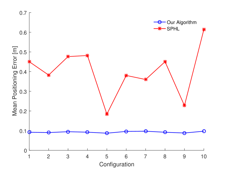
Figure 1: For variable anchor positioning, our algorithm has a constant and better performance than the SPHL, which highly depends on the network configuration. The resultant MPE is the average of 100 MC trials, where distance measurements noise has an STD of $0.2m$ and bearing noise an equivalent STD of $2\degree$.

4 Dynamic Formulation

While the previous formulation is adequate for static networks, when vehicles perform a trajectory, it is beneficial to take into account different consecutive positions to obtain a better estimate. Therefore, we introduce a time window and consider that each vehicle $i$ has access to its own velocity $\beta_{i}(t)$ at time $t$.

In order to model velocity measurements, we decompose them into a unit vector $v_{i}(t)$ and magnitude $V_{i}(t)$. Under this format, we can look at $V_{i}(t)\Delta T$, the distance travelled by one node during a time interval $\Delta T$, as the distance between two points $x_{i}(\tau)$ and $x_{i}(\tau-1)$. Besides, the unit vector $v_{i}(t)$ can be thought of as the bearing between those same nodes, $x_{i}(\tau)$ and $x_{i}(\tau-1)$, usually denoted as heading. Essentially, this means that we have distance and bearing measurements just as in the previous formulation, except that they exist between the same node at different time instants. So, we can model them in a similar way, with $V_{i}(t)\Delta T$ following a Gaussian distribution with variance $\sigma_{i}^{2}$ and $v_{i}(t)$ following a von Mises-Fisher distribution with concentration parameter $\varkappa_{i}$.

Therefore, we obtain a formulation with similar structure to Problem (1), which can be relaxed in the same manner, by introducing an additional variable $s$, with the same role as $y$. We define the concatenation of the optimization variables over nodes or edges at instant $\tau$ as $x(\tau)=\{x_{i}(\tau)\}_{i\in\mathcal{V}}$, $y(\tau)=\{y_{ij}(\tau)\}_{i\sim j}$, $s(\tau)=\{s_{i}(\tau)\}_{i\in\mathcal{V}}$, $w_{i}(\tau)=\{w_{ik}(\tau)\}_{k\in\mathcal{A}_{i}}$, $w(\tau)=\{w_{i}(\tau)\}_{i\in\mathcal{V}}$. Similarly, the concatenation over a time window of size $T_{0}$ at time $t$ is given as $x=\{x(\tau)\}_{t-T_{0}\leq\tau\leq t}$, $y=\{y(\tau)\}_{t-T_{0}\leq\tau\leq t}$ , $s=\{s(\tau)\}_{t-T_{0}\leq\tau\leq t}$ and $w=\{w(\tau)\}_{t-T_{0}\leq\tau\leq t}$. Note that the dependency on $t$ (the time instant) is omitted from the notation in all variables ($x,y,s,w$) for compactness. The final problem is given as

$$\begin{split}\operatornamewithlimits{minimize}_{x,y,w,s}&\quad f_{\textrm{dist}}(x,y,w)+f_{\textrm{ang}}(y,w)\\ &+f_{\textrm{vel}}(x,s)\\ \operatornamewithlimits{\text{subject to}}&\quad\|y_{ij}(\tau)\|\leq d_{ij}(\tau),\quad\|w_{ik}(\tau)\|\leq r_{ik}(\tau),\\ &\quad\|s_{i}(\tau)\|\leq V_{i}(\tau)\Delta T,\end{split}$$ (9)

where

$$\begin{split}f_{\textrm{vel}}&(x,s)=\\ &\sum_{i\in\mathcal{V}}\sum_{\tau=t-T_{0}+1}^{t}\frac{1}{2\sigma_{i}^{2}}\big{(}\|x_{i}(\tau)-x_{i}(\tau-1)-s_{i}(\tau)\|\big{)}^{2}\\ &-\sum_{i\in\mathcal{V}}\sum_{\tau=t-T_{0}+1}^{t}\varkappa_{i}\Bigg{(}v_{i}(\tau)^{T}\frac{s_{i}(\tau)}{V_{i}(\tau)\Delta T}\Bigg{)}\quad,\end{split}$$ (10)

$$\begin{split}f_{\textrm{dist}}&(x,y,w)=\\ &\sum_{i\sim j\in\mathcal{E}^{d}}\sum_{\tau=t-T_{0}}^{t}\frac{1}{2\sigma_{ij}^{2}}\big{(}\|x_{i}(\tau)-x_{j}(\tau)-y_{ij}(\tau)\|\big{)}^{2}\\ &\sum_{i\in\mathcal{V}}\sum_{k\in\mathcal{A}^{d}_{i}}\sum_{\tau=t-T_{0}}^{t}\frac{1}{2\varsigma_{ik}^{2}}\big{(}\|x_{i}(\tau)-a_{k}(\tau)-w_{ik}(\tau)\|\big{)}^{2}\end{split}$$ (11)

and

$$\begin{split}f_{\textrm{ang}}&(y,w)=\\ &-\sum_{i\sim j\in\mathcal{E}^{u}}\sum_{\tau=t-T_{0}}^{t}\Bigg{(}\varkappa_{ij}u_{ij}(\tau)^{T}\frac{y_{ij}(\tau)}{d_{ij}(\tau)}\Bigg{)}\\ &-\sum_{i\in\mathcal{V}}\sum_{k\in\mathcal{A}^{u}_{i}}\sum_{\tau=t-T_{0}}^{t}\Bigg{(}\lambda_{ik}q_{ik}(\tau)^{T}\frac{w_{ik}(\tau)}{r_{ik}(\tau)}\Bigg{)}.\end{split}$$ (12)

4.1 Reformulation

We shall now reformulate (9) in matrix notation. Let $\Sigma_{N}$ be the diagonal matrix of $\frac{1}{\sigma_{ij}}$. Then, the first term of (11) can be written as

$$f_{\textrm{dist,nodes}}(x,y)=\frac{1}{2}\|\Sigma_{N}Ax-\Sigma_{N}y\|^{2}\quad,$$ (13)

where matrix $A$ is the Kronecker product of the identity matrix of dimension $T_{0}$ with the result from the Kronecker product of $C$, the arc-node incidence matrix of the network, with identity matrix of dimension $p$, that is,

$$A=I_{T_{0}}\otimes(C\otimes I_{p})=(I_{T_{0}}\otimes C)\otimes I_{p}.$$ (14)

Essentially, this extends matrix $C$ along the dimension of the problem ($p$) and time window ($T_{0}$), assuming the set of edges remains constant over $T_{0}$.

In the same way, taking $\Sigma_{V}$ to be the diagonal matrix of $\frac{1}{\sigma_{i}}$, the first term of (10) may be written as

$$f_{\textrm{dist,vel}}(x,s)=\frac{1}{2}\|\Sigma_{V}Nx-\Sigma_{V}s\|^{2}$$ (15)

where $N=C_{\textrm{vel}}\otimes I_{p}$. However, it should be clearly noted that, in this formulation, the set of edges has changed, hence the different designation $C_{\textrm{vel}}$. Each node at time $t$ has an edge with its position at $t-1$ and $t+1$, except for the first and last instants of the time window. The last distance term, concerning anchor-node measurements, may be reformulated as

$$f_{\textrm{dist,anchors}}(x,w)=\frac{1}{2}\|\Sigma_{A}Ex-\Sigma_{A}\alpha-\Sigma_{A}w\|^{2}$$ (16)

where vectors for anchor positions are concatenated in the usual way as $\alpha_{i}(\tau)=\{a_{ik}(\tau)\}_{k\in\mathcal{A}_{i}}$, $\alpha(\tau)=\{\alpha_{i}(\tau)\}_{i\in\mathcal{V}}$, $\alpha=\{\alpha(\tau)\}_{t-T_{0}\leq\tau\leq t}$. $E$ is a selector matrix, indicating which node has a measurement relative to each anchor and $\Sigma_{A}$ the diagonal matrix of $\frac{1}{\varsigma_{ik}}$.

Finally, the angle measurements are grouped as $\tilde{u}_{ij}(\tau)=\frac{\varkappa_{ij}u_{ij}(\tau)}{d_{ij}(\tau)}$, $\tilde{q}_{ik}(\tau)=\frac{\lambda_{ik}q_{ik}(\tau)}{r_{ik}(\tau)}$ and $\tilde{v}_{i}(\tau)=\frac{\varkappa_{i}v_{i}(\tau)}{V_{i}(\tau)\Delta T}$. Following the same reasoning as before, $u(\tau)=\{\tilde{u}_{ij}(\tau)\}_{i\sim j}$, $v(\tau)=\{\tilde{v}_{i}(\tau)\}_{i\in\mathcal{V}}$ and $q_{i}(\tau)=(\tilde{q}_{ik}(\tau))_{k\in\mathcal{A}_{i}}$, $q(\tau)=\{q_{i}(\tau)\}_{i\in\mathcal{V}}$. Then, concatenating along the time window, $u=\{u(\tau)\}_{t-T_{0}\leq\tau\leq t}$ , $v=\{v(\tau)\}_{t-T_{0}\leq\tau\leq t}$ and $q=\{q(\tau)\}_{t-T_{0}\leq\tau\leq t}$. It follows that

$$f_{\textrm{ang}}(y,w,s)=-u^{T}y-q^{T}w-v^{T}s.$$ (17)

Considering the definitions in (13), (15), (16) and (17), Problem (9) is reformulated as

$$\begin{split}\operatornamewithlimits{minimize}_{x,y,w,s}&\quad f_{\textrm{dist,nodes}}(x,y)+f_{\textrm{dist,anchors}}(x,w)+\\ &f_{\textrm{dist,vel}}(x,s)+f_{\textrm{ang}}(y,w,s)\\ \operatornamewithlimits{\text{subject to}}&\quad\|y_{ij}(\tau)\|\leq d_{ij}(\tau),\quad\|w_{ik}(\tau)\|\leq r_{ik}(\tau),\\ &\quad\|s_{i}(\tau)\|\leq V_{i}(\tau)\Delta T\end{split}$$ (18)

Introducing a variable $z=(x,y,w,s)$ and defining $\mathcal{Z}=\{z:\|y_{ij}(t)\|\leq d_{ij}(t),i\sim j\in\mathcal{V};\|w_{ik}(t)\|\leq r_{ik}(t),i\in\mathcal{V},k\in\mathcal{A}_{i};\|s_{i}(t)\|\leq V_{i}(t)\Delta T,i\in\mathcal{V}\}$, Problem (18) can be written in a quadratic form as

$$\operatornamewithlimits{minimize}_{z}\quad\frac{1}{2}z^{T}Mz-b^{T}z$$ (19)

$$\operatornamewithlimits{\text{subject to}}\quad z\in\mathcal{Z}$$

where $M=M_{1}+M_{2}+M_{3}$, with

$$M_{1}=\begin{bmatrix}A^{T}\Sigma_{N}\\ -\Sigma_{N}\\ 0\\ 0\end{bmatrix}\begin{bmatrix}\Sigma_{N}A&-\Sigma_{N}&0&0\end{bmatrix}\quad,$$

$$M_{2}=\begin{bmatrix}E^{T}\Sigma_{A}\\ 0\\ -\Sigma_{A}\\ 0\end{bmatrix}\begin{bmatrix}\Sigma_{A}E&0&-\Sigma_{A}&0\end{bmatrix}\quad,$$

$$M_{3}=\begin{bmatrix}N^{T}\Sigma_{V}\\ 0\\ 0\\ -\Sigma_{V}\end{bmatrix}\begin{bmatrix}\Sigma_{V}N&0&0&-\Sigma_{V}\end{bmatrix}\quad,$$

and $b=b_{1}+b_{2}$, with

$$b_{1}=\begin{bmatrix}E^{T}\Sigma_{A}\\ 0\\ -\Sigma_{A}I\\ 0\end{bmatrix}\Sigma_{A}\alpha$$

and

$$b_{2}=\begin{bmatrix}0\\ u\\ q\\ v\end{bmatrix}\quad.$$

5 Distributed Implementation

Minimization of the convex problem in (19) can be carried out in multiple ways. However, we strive for a method suitable for distributed settings. Hence, we choose the Fast Iterative Shrinkage-Thresholding Algorithm (FISTA) [3], which is an extension of the gradient method and will produce a naturally distributed solution.

FISTA handles problems defined as

$$\operatornamewithlimits{minimize}_{x}f(x)=g(x)+h(x)$$ (20)

where $g(x):\mathbb{R}^{n}\rightarrow\mathbb{R}$ is a smooth convex function, continuously differentiable with Lipschitz continuous gradient $L$, and $h(x)$ is a closed and convex function with an inexpensive proximal operator with parameter $t_{k}$, expressed as $\textrm{prox}_{t_{k}h}$. Under these assumptions, FISTA’s solution for Problem (20) is given iteratively as

$$y=x^{\left(k-1\right)}+\frac{k-2}{k+1}\Big{(}x^{\left(k-1\right)}-x^{\left(k-2\right)}\Big{)}$$ (21)

$$x^{\left(k\right)}=\textrm{prox}_{t_{k}h}(y-t_{k}\nabla g(y))\quad.$$

This method has a convergence rate $f(x^{\left(k\right)})-f^{*}$ (where $f^{*}$ is the optimal value) of $\mathcal{O}(1/k^{2})$, for a fixed step size of $t_{k}=1/L$.

5.1 Implementation

For Problem (19) to be solved with FISTA, it is necessary to define $g(x)$ and $h(x)$, along with $\textrm{prox}_{t_{k}h}$ and $t_{k}$. In this case, $g(x)$ is the quadratic cost function $\frac{1}{2}z^{T}Mz-b^{T}z$. It is noted that a function is said to have a Lipschitz Continuous Gradient with Lipschitz constant $L$ if the following condition is true

$$\|\nabla f(x)-\nabla f(y)\|\leq L\|x-y\|$$ (22)

and quadratic functions have a Lipschitz continuous gradient. Besides, the required gradient $\nabla g(z)$ is straightforward, given as $\nabla g(z)=Mz-b$.

Term $h(x)$ corresponds to the indicator function $I_{\mathcal{Z}}(z)$ for set $\mathcal{Z}$, defined as

$$I_{\mathcal{Z}}(z)=\begin{cases}0,\qquad\text{if }z\in\mathcal{Z}\\ +\infty,\quad\text{otherwise}\end{cases}$$

and to obtain $\textrm{prox}_{t_{k}h}$ of an indicator function, we refer to [25]. When $h(x)$ is indicator function of closed convex set $\mathcal{Z}$, then $\textrm{prox}_{t_{k}h}$ is the projection of $z$ on set $\mathcal{Z}$, $P_{\mathcal{Z}}(x)$, defined as

$$P_{\mathcal{Z}}(z)=\operatornamewithlimits{argmin}_{x\in\mathcal{Z}}\|x-z\|^{2},$$

which for our constraints with general structure $\{z:\|z\|\leq d\}$ is implemented as

$$P_{\mathcal{Z}}(z)=\begin{cases}z,\quad\textrm{if}\quad\|z\|\leq d\\ \frac{z}{\|z\|}d,\quad\textrm{if}\quad\|z\|>d\quad.\end{cases}$$

Finally, it is necessary to obtain a value for $1/L$, where $L$ is the Lipschitz constant of function $\frac{1}{2}z^{T}Mz-b^{T}z$. Resorting to [33], we obtain an upper-bound for $L$ as (see Appendix A for the complete derivation)

$$\begin{split}L&\leq\tfrac{1}{\sigma_{N}^{2}}2\delta_{\textrm{max}}+\tfrac{1}{\sigma_{A}^{2}}\max_{i\in\mathcal{V}}|\mathcal{A}_{i}|+\tfrac{1}{\sigma_{V}^{2}}2\delta^{V}_{\textrm{max}}(T)+K\end{split}\quad,$$

where $\delta_{\textrm{max}}$ is the maximum node degree of the network and $\delta^{V}_{\textrm{max}}$ is either $2$ for any $T>2$, $1$ for $T=2$ and $0$ for no time window ($T=1$). The term $\max_{i\in\mathcal{V}}|\mathcal{A}_{i}|$ corresponds to the maximum number of anchors connected to a node. Finally, $K=\tfrac{1}{\sigma_{N}^{2}}+\tfrac{1}{\sigma_{A}^{2}}+\tfrac{1}{\sigma_{V}^{2}}$, where $\sigma_{N}$, $\sigma_{A}$ and $\sigma_{V}$ are the maximum values of matrices $\Sigma_{N}$, $\Sigma_{A}$ and $\Sigma_{V}$, respectively. The distributed computation of $L$ can be attained, as suggested in [33], by a diffusion algorithm.

In the end, we obtain a distributed method, made explicit in Algorithm 1 (see the full derivation in Appendix B). We define $C_{(i\sim j,i)}$ as the element of $C$ on row referring to edge $i\sim j$ and column referring to node $i$; $N_{i}$ as the sub-matrix of $N$, whose rows correspond to node $i$; $\textbf{s}_{i}$ and $\textbf{x}_{i}$ as the concatenation of $s_{i}(\tau)$ and $x_{i}(\tau)$ over the time window; $\textbf{w}_{i}$ and $\textbf{y}_{i}$ as the concatenation of $w_{ik}(\tau)$ and $y_{ij}(\tau)$ over the respective edges and time window. Besides, the projections for each component are defined as $\mathcal{Y}_{ij}(t)=\{y_{ij}(t):\|y(t)\|\leq d_{ij}(t)\}$, $\mathcal{W}_{ik}(t)=\{w_{ik}(t):\|w_{ik}(t)\|\leq r_{ik}(t)\}$ and $\mathcal{S}_{i}(t)=\{s_{i}(t):\|s_{i}(t)\|\leq v_{i}(t)\}$. The elements $F_{1}(\tau)$ through $F_{4}(\tau)$ for the update of $x_{i}^{\kappa+1}(\tau)$ are given as

$$F_{1}(\tau)=\hat{x}_{i}^{\kappa}(\tau)\Big{(}L-\sum_{i\sim j\in\mathcal{E}_{i}}\frac{1}{\sigma_{ij}^{2}}-\sum_{k\in\mathcal{A}_{i}}\frac{1}{\varsigma_{ik}^{2}}\Big{)},$$

$$F_{2}(\tau)=\sum_{i\sim j\in\mathcal{E}_{i}}\frac{1}{\sigma_{ij}^{2}}(\hat{x}_{j}^{\kappa}(\tau)+C_{(i\sim j,i)}(\tau)\hat{y}_{ij}^{\kappa}(\tau)),$$

$$F_{3}(\tau)=\sum_{k\in\mathcal{A}_{i}}\frac{1}{\varsigma_{ik}^{2}}(\hat{w}_{ik}^{\kappa}(\tau)+\alpha_{k}(\tau))$$

and

$$F_{4}(\tau)=\big{[}N_{i}^{T}\Sigma_{V}^{2}(\hat{\textbf{s}}_{i}^{\kappa}-N_{i}\hat{\textbf{x}}_{i}^{\kappa})\big{]}_{\tau},$$

where $\big{[}v\big{]}_{\tau}$ is the element of a vector $v$, relative to instant $\tau$. The update is split into four terms for convenience of the reader: $F_{1}(\tau)$ relates to the node position; $F_{2}(\tau)$ and $F_{3}(\tau)$ relate to distance edges between the node and its neighbor nodes or anchors (respectively); and $F_{4}(\tau)$ to the node velocity. Recalling that we stay under a convex formulation, it is noted that $z^{0}$ may be initialized with any feasible value.

We emphasize that each node on the network computes its own estimate, relying only on distances and angles taken with respect to its neighbors (nodes or anchors) and on its own velocity measurements. Notice that quantities related to other nodes are always within the set $\mathcal{A}_{i}$ (neighbor anchors of node $i$) or $\mathcal{E}_{i}$ (neighbor nodes of node $i$). At end of each iteration, nodes also need to share their current estimates, but since this is only needed amongst neighbors, the method remains distributed.

Algorithm 1 Hybrid Convex Localization

0:  $L$;

  $\{d_{ij}(t),u_{ij}(t):i\sim j\in\mathcal{E}\}$; $\{r_{ik}(t),q_{ik}(t):i\in\mathcal{V},k\in\mathcal{A}\}$; $\{v_{i}(t)\in\mathcal{V}\}$

  $\hat{x}=\{\hat{x}_{i}\}$

  Choose $z^{0}=(x^{0},y^{0},w^{0},s^{0})=0$;

  for all t do

     $\kappa=1$; $z^{1}=z^{0}$

     while some stopping criterion is not met, each node $i$ do

        $\hat{z}_{i}^{\kappa}=z_{i}^{\kappa}+\frac{\kappa-1}{\kappa}(z_{i}^{\kappa}-z_{i}^{\kappa-1})$

        for all $t-T_{0}\leq\tau\leq t$ do

           $x_{i}^{\kappa+1}(\tau)=\frac{1}{L}\Big{[}F_{1}(\tau)+F_{2}(\tau)+F_{3}(\tau)+F_{4}(\tau)\Big{]}$

        end for

        for all $i\sim j\in\mathcal{E}_{i}$ and $t-T_{0}\leq\tau\leq t$ do

           $y_{ij}^{\kappa+1}(\tau)=P_{\mathcal{Y}_{ij}(\tau)}\Big{(}\frac{L-1/\sigma_{ij}^{2}}{L}\hat{y}_{ij}^{\kappa}(\tau)+\frac{\tilde{u}_{ij}(\tau)}{L}+\frac{1}{L\sigma_{ij}^{2}}C_{(i\sim j,i)}(\tau)(\hat{x}_{i}^{\kappa}(\tau)-\hat{x}_{j}^{\kappa}(\tau))\Big{)}$

        end for

        for all $k\in\mathcal{A}_{i}$ and $t-T_{0}\leq\tau\leq t$ do

           $w_{ik}^{\kappa+1}(\tau)=P_{\mathcal{W}_{ik}(\tau)}\Big{(}\frac{L-1/\varsigma_{ik}^{2}}{L}\hat{w}_{ik}^{\kappa}(\tau)+\frac{1}{L\varsigma_{ik}^{2}}(\hat{x}_{i}^{\kappa}(\tau)-a_{k}(\tau))+\frac{\tilde{q}_{ik}(\tau)}{L}\Big{)}$

        end for

        if $T_{0}>1$ then

           for all $t-T_{0}+1\leq\tau\leq t$ do

              $s_{i}^{\kappa+1}(\tau)=P_{\mathcal{S}_{i}}\Big{(}\frac{L-1/\sigma_{ij}^{2}}{L}+\frac{1}{L\sigma_{i}^{2}}(\hat{x}_{i}^{\kappa}(\tau)-\hat{x}_{i}^{\kappa}(\tau-1))+\frac{\tilde{v}_{i}(\tau)}{L}\Big{)}$

           end for

        end if

        $z_{i}^{\kappa+1}=(\textbf{x}_{i}^{\kappa+1},\textbf{y}_{i}^{\kappa+1},\textbf{w}_{i}^{\kappa+1},\textbf{s}_{i}^{\kappa+1})$

        $\kappa=\kappa+1$

        broadcast $x_{i}$ to all neighbors

     end while

     

     return  $\hat{x}=\{\textbf{x}_{i}^{\kappa+1}\}$

  end for

6 Parameter Estimation

Until this point, the parameters $\sigma$ and $\varkappa$ of error distributions have been assumed to be known a priori. In real applications, these parameters could be estimated from previous experiments. However, this can also be included in the algorithm so that no previous knowledge is necessary. With each new measurement, a new estimate for $\varkappa$ and $\sigma$ is computed, which is desired to converge to the true value.

Maximum likelihood estimators for the parameters of each distribution are easily found in the literature. Given a random variable X, normally distributed with unknown mean and variance $\sigma^{2}$, the MLE for the latter parameter is given as [22]

$$\hat{\sigma}^{2}=\frac{1}{n-1}\sum_{i=1}^{n}(X_{i}-\bar{X})^{2}.$$ (23)

For the estimation of the concentration parameter $\varkappa$, authors in [2], propose the use of

$$\hat{\varkappa}=\frac{\bar{\gamma}(p-\bar{\gamma}^{2})}{1-\bar{\gamma}^{2}},$$ (24)

where $\bar{\gamma}=\frac{\|\sum_{i=1}^{n}x_{i}\|}{n}$, $x_{i}$ are independent and identically distributed sample unit vectors drawn from a Von Mises-Fisher distribution $vMF(\mu,\kappa)$ and $p$ is the dimension of $x_{i}$.

6.1 Implementation

Evidently, there is no access to the true values of our measurements to accurately estimate $\varkappa$ and $\sigma$. However, after each computation of position estimates by the algorithm, it is possible to compute estimated distances, angles and velocities which can be used as the "true value". So, exact values of $\varkappa$ and $\sigma$ are not to be expected but if the position estimates are close to the true ones, then a similar value should be obtained. However, note that these two estimators influence each other and poor estimates in one will affect the other.

Denoting by $\hat{x}$ the value obtained from our position estimation, it is possible to compute the resulting distances and bearings as

$$\hat{d}_{ij}(t)=\|\hat{x}_{i}(t)-\hat{x}_{j}(t)\|$$

and

$$\hat{u}_{ij}(t)=\frac{\hat{x}_{i}(t)-\hat{x}_{j}(t)}{\|\hat{x}_{i}(t)-\hat{x}_{j}(t)\|}.$$

Given the obtained measurements $d_{ij}$, (23) can now be used for variance estimation as

$$\hat{\sigma}_{ij}^{2}(t)=\frac{1}{t}\sum_{\tau=1}^{t}(d_{ij}(\tau)-\hat{d}_{ij}(\tau))^{2}$$

and, given bearing measurements $u_{ij}$, (24) is used for concentration parameter estimation as

$$\hat{\varkappa}_{ij}(t)=\frac{\bar{\gamma}_{ij}(t)(p-\bar{\gamma}_{ij}^{2}(t))}{1-\bar{\gamma}_{ij}(t)^{2}}\quad,$$

where

$$\bar{\gamma}_{ij}(t)=\frac{1}{t}\Bigg{\lVert}\sum_{\tau=1}^{t}\frac{u_{ij}(\tau)-\hat{u}_{ij}(\tau)}{\|u_{ij}(\tau)-\hat{u}_{ij}(\tau)\|}\Bigg{\rVert}.$$ (25)

The same reasoning can be applied to node-anchor edges, with similar resulting equations.

Velocity measurements ($\beta_{i}$) require a more careful approach, given that a similar process using $\hat{\beta}_{i}(t)\Delta T=x_{i}(t)-x_{i}(t-1)$ does not produce good results. This problem is considered in [30] and the proposed solution is based on central finite differences with a time lag and rejection of high-frequency noise. The proposed estimation is then given as

$$\hat{\beta}_{i}(t)\Delta T= \frac{5(x_{i}(t-3)-x_{i}(t-5))}{32}+$$ (26)

$$\frac{4(x_{i}(t-2)-x_{i}(t-6))}{32}+$$

$$\frac{(x_{i}(t-1)-x_{i}(t-7))}{32}.$$

It should be noted that the introduction of a time lag has practical consequences during implementation, that should be taken into account. Recalling that $\hat{\beta}_{i}(t)$ is decomposed as $\hat{\beta}_{i}(t)=\hat{v}_{i}(t)\hat{V}_{i}(t)$, estimates for variance and concentration are given as

$$\hat{\sigma}_{i}^{2}(t)=\frac{1}{t}\sum_{\tau=1}^{t}(V_{i}(\tau)-\hat{V}_{i}(\tau))^{2}$$ (27)

and

$$\hat{\varkappa}_{i}(t)=\frac{\bar{\gamma}_{i}(t)(p-\bar{\gamma}_{i}^{2}(t))}{1-\bar{\gamma}_{i}^{2}(t)}\quad,$$ (28)

with $\bar{\gamma}_{i}(t)=\frac{\|\sum_{\tau=1}^{t}v_{i}(\tau)-\hat{v}_{i}(\tau)\|}{t}$.

The addition of parameter estimation to Algorithm 1 produces a final distributed and parameter-free algorithm, which can be found in Appendix C.

7 Simulation Results

We compare our algorithm with EKF, the standard method with an equivalent data model. EKF requires initialization, for which we use the true position with a Standard Deviation (STD) of 2 m. We also optimize its parameters for the considered trajectories, through grid search.

In order to evaluate the localization accuracy, we use the Mean Navigation Error (MNE) defined as

$$\text{MNE}(\hat{x},t)=\frac{1}{MN}\sum_{m=1}^{M}\sum_{i=1}^{N}\|\hat{x}^{m}_{i}(t)-x^{m}_{i}(t)\|_{2}\quad,$$

where $\hat{x}$ is an estimate of $x$, $M$ the number of Monte Carlo trials, $N$ the number of unknown nodes and $T$ the time interval.

Considering noise levels obtainable with current instrumentation, we define $\sigma_{d}=0.5~{}\text{m}$ (for all distance measurements), $\sigma_{v}=0.1~{}\text{m}/s$ (for all speed measurements), $\kappa_{a}=1000$ (for all bearing measurements) and $\kappa_{v}=1000$ (for all heading measurements). For this first section, we provide both methods (our algorithm and EKF) with the true values of noise deviation. In the second part, we test the final parameter-free algorithm.

7.1 Lawnmower trajectory

A common trajectory in AUV missions is the Lawnmower, as depicted in Figure 2. Figure 3 represents the MNE for each algorithm along the lawnmower trajectory. It is clear that, unlike EKF, our method is able to keep a constant error regardless of the vehicles’ movement. While EKF slightly outperforms our method during linear parts, the inverse is observed for the remaining trajectory.

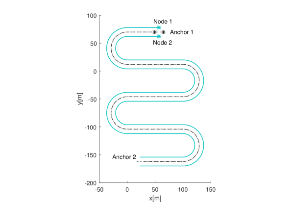
Figure 2: Lawnmower trajectory with two nodes, in a solid blue line, travelling on both sides of two anchors, in dashed and dotted black lines. Note that both anchors describe similar trajectories but one is "behind" the other. The beginning of each trajectory is marked with a star.

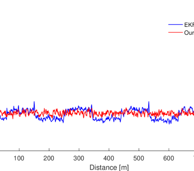
Figure 3: Comparison of Mean Navigation Error between EKF and our algorithm, during a lawnmower trajectory, averaged over 100 MC trials. The curved segments of the trajectory are evidenced by the higher error in EKF, where our method outperforms it. For the linear parts, EKF shows better accuracy.

7.2 Outliers during the lap trajectory

When we consider a more realistic case of outliers in measurements, the difference in performance increases. This is implemented by introducing a distance measurement with value $5d$ with a probability of $10\%$, where $d$ is the true distance. Ranges between the outer node and one of the anchors are contaminated with outliers, evidenced by the peaks in position estimates (Figure 4). The line in red, representing results from our algorithm, presents smaller variations with outliers and does not require as much time as EKF (in blue) to recover. The difference between them also seems to accentuate during non-linear trajectory parts.

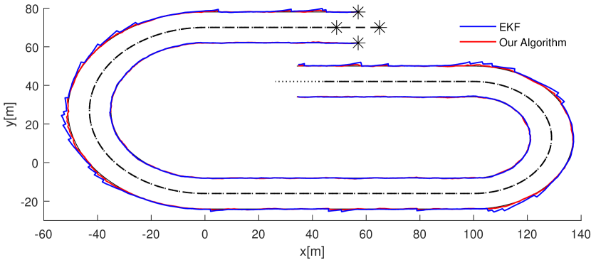
Figure 4: Distances between one of the anchors (dashed lines) and the outer node, are contaminated with outliers, evidenced by the peaks in both estimates. EKF, in blue, presents larger peaks, showing to be less robust than our algorithm, in red.

We further extend this scenario to the situation where all range measurements related to the outer node are subject to outliers, not only with both anchors but also with the second node. The results, shown in Figure 5, reveal an even greater difference between both performances, with our algorithm attaining superior robustness.

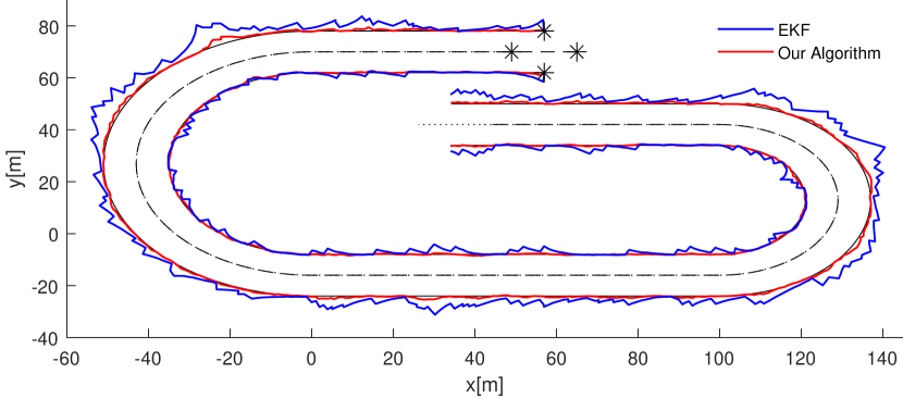
Figure 5: Distances between the outer node and all the other vehicles are contaminated with outliers. EKF, in blue, is affected to a higher extent by this problem and takes more time to recover from it than our algorithm, in red. The results are obtained during a lap trajectory performed by two anchors, in dashed lines, and two nodes, in black lines, with initial positions marked as a star.

7.3 3D Helix trajectory with parameter estimation

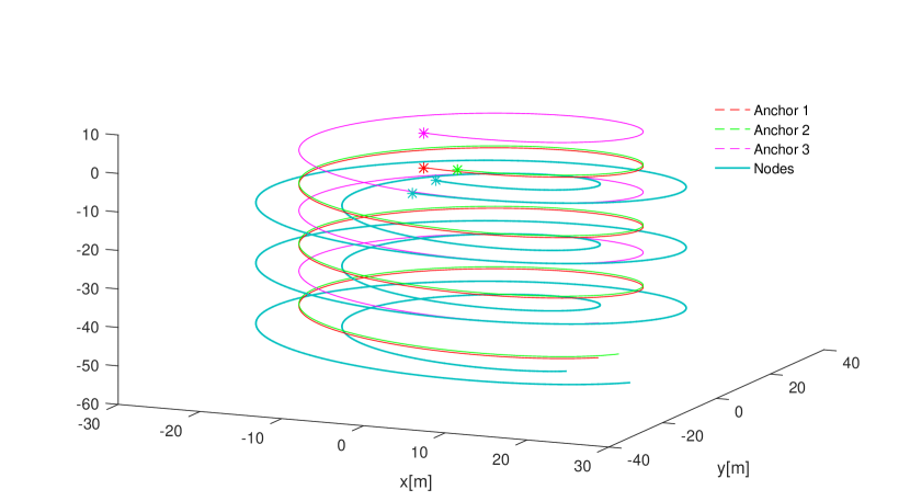
Figure 6: Helix trajectory with two nodes, in a solid blue line, travelling on both sides of three anchors, in dashed lines of different colors. The start of each trajectory is marked with a star. All paths maintain the same velocity in the $x$ and $y$ axis, progressively decreasing the $z$ component.

In Figure 7, we present the evolution of $\hat{\sigma}_{d}$ for all the distance measurements, where the true $\sigma_{d}$ was set to $0.5m$. The estimates converge to $\sigma_{d}$, as desired, but it should be noted that a considerable number of measurements is necessary before this happens. Consequently, we choose a default initial value for all $\sigma$ and $\kappa$ (different from the real one), to be used during the first time steps of the trajectory. After that point, the estimated values are used instead. The introduction of parameter estimation does not seem to considerably decrease performance when compared with an optimal case of known values, as Figure 8 expresses.

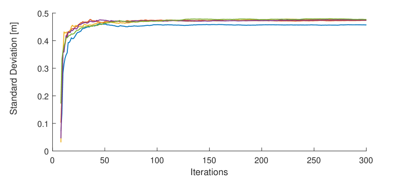
Figure 7: Evolution of estimates of $\hat{\sigma}_{d}$ for distance measurements. After some time, the estimates converge to values close to the true $\sigma_{d}=0.5m$. The different lines correspond to $\sigma_{ij}$ for different edges, all with the same value of STD. Note that parameter estimation does not start at iteration 0 due to the time lag in velocity estimation.

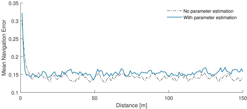
Figure 8: Comparison of performance between the method with parameter estimation and the optimal case, where the real parameter values are provided. Although the latter stays slightly below the former for most of the trajectory, the difference is almost negligible.

8 Concluding Remarks

We presented an MLE formulation for a generic network localization problem, both in static and dynamic contexts, including range and bearing measurements between nodes. The introduction of angular information with an appropriate relaxation allowed the method to overcome some challenges usually encountered in similar relaxations for distances. For example, anchors are not required to be deployed at the boundary of the network, unlike many other approaches. When compared with a hybrid state-of-the-art SDP relaxation, our algorithm reveals superior accuracy and less susceptibility to network configuration. While it is not necessary that all nodes measure bearings, it must be emphasized that each bearing should have corresponding distance measurement. Of course, range measurements can exist alone for some pairs of vehicles. This is due to our relaxation, causing these terms to be dependent on the formulation for the ranges.

The initial formulation is extended to dynamic networks, in a horizon-based approach, and proven to be distributed. Comparison with EKF (Figure 5), a centralized state-of-the-art method, shows the superior performance of our method for cases with variable motion patterns, where for mostly linear trajectories the EKF still slightly outperforms our distributed estimator. Nonetheless, EKF requires a good initialization for convergence, whereas our distributed convex method is proven to converge without initialization requirements. Furthermore, the accuracy of our algorithm is nearly constant throughout the trajectory, thus being more predictable than EKF. More importantly, our algorithm shows more robustness in the presence of outliers in measurements, which is a known issue in real-life scenarios.

Besides, with the proposed parameter estimation process, no parameter tuning is required, so the algorithm can be easily applied to new environments or technologies. However, it should be noted that this is a sensitive step where abnormal values could start a chain of wrong position estimates, leading to equally wrong parameter estimates and so on. While a formal proof would be desirable in future approaches, our simulations have consistently demonstrated that the method maintains its performance, regardless of the initialization chosen and despite the estimated parameters. Therefore, we have strong empirical evidence of robustness for the proposed method, although additional research is needed to prove its validity formally.

Appendix A Upper bound on Lipschitz Constant

First, the gradient difference is manipulated until an expression with the structure of (22) is obtained as

$$\begin{split}\|\nabla f(x)-\nabla f(y)\|&=\|(Mx-b)-(My-b)\|\\ &=\|M(x-y)\|\\ &\leq\|M\|\|(x-y)\|\quad.\end{split}$$ (29)

The last step of Equation (29) corresponds to the definition of Lipschitz continuity with $L=\|M\|$, where $\|M\|$ is the matrix norm of $M$ defined as

$$\|M\|=\sup\Bigg{\{}\frac{\|Mx\|}{\|x\|}:x\in R^{n},|x|\neq 0\Bigg{\}}\quad.$$

Further manipulations are necessary to obtain a bound for this constant; these are shown in (30) and the justification is presented below.

$$\begin{split}L=&\|M\|\\ \stackrel{{\scriptstyle\textrm{1}}}{{\leq}}&\|M_{1}\|+\|M_{2}\|+\|M_{3}\|\\ \stackrel{{\scriptstyle\textrm{2}}}{{=}}&\sqrt{\lambda_{\textrm{max}}(M_{1}^{T}M_{1})}+\sqrt{\lambda_{\textrm{max}}(M_{2}^{T}M_{2})}+\sqrt{\lambda_{\textrm{max}}(M_{3}^{T}M_{3})}\\ \stackrel{{\scriptstyle\textrm{3}}}{{=}}&\lambda_{\textrm{max}}(M_{1})+\lambda_{\textrm{max}}(M_{2})+\lambda_{\textrm{max}}(M_{3})\\ \stackrel{{\scriptstyle\textrm{4}}}{{=}}&\lambda_{\textrm{max}}(\Sigma_{N}^{2}AA^{T}+\Sigma_{N}^{2})+\lambda_{\textrm{max}}(\Sigma_{A}^{2}EE^{T}+\Sigma_{A}^{2})\\ &+\lambda_{\textrm{max}}(\Sigma_{V}^{2}NN^{T}+\Sigma_{V}^{2})\\ \stackrel{{\scriptstyle\textrm{5}}}{{\leq}}&\lambda_{\textrm{max}}(\Sigma_{N}^{2}AA^{T})+\lambda_{\textrm{max}}(\Sigma_{A}^{2}EE^{T})+\lambda_{\textrm{max}}(\Sigma_{V}^{2}NN^{T})\\ &+\lambda_{\textrm{max}}(\Sigma_{N}^{2})+\lambda_{\textrm{max}}(\Sigma_{A}^{2})+\lambda_{\textrm{max}}(\Sigma_{V}^{2})\\ \stackrel{{\scriptstyle\textrm{6}}}{{\leq}}&\tfrac{1}{\sigma_{N}^{2}}\lambda_{\textrm{max}}(AA^{T})+\tfrac{1}{\sigma_{A}^{2}}\lambda_{\textrm{max}}(EE^{T})+\tfrac{1}{\sigma_{V}^{2}}\lambda_{\textrm{max}}(NN^{T})\\ &+(\tfrac{1}{\sigma_{N}^{2}}+\tfrac{1}{\sigma_{A}^{2}}+\tfrac{1}{\sigma_{V}^{2}})\\ \end{split}$$ (30)

• $\stackrel{{\scriptstyle\textrm{1}}}{{}}$ For 2 matrices $A$ and $B$, $\|A+B\|\leq\|A\|+\|B\|$ (triangle inequality)

• $\stackrel{{\scriptstyle\textrm{2}}}{{}}$ $\|A\|=\sqrt{\lambda_{\textrm{max}}(A^{T}A)}$

• $\stackrel{{\scriptstyle\textrm{3}}}{{}}$ $M_{1}$,$M_{2}$ and $M_{3}$ are symmetric ($A^{T}=A$), thus verifying $\sqrt{\lambda_{\textrm{max}}(A^{T}A)}=\lambda_{\textrm{max}}(A)$

• $\stackrel{{\scriptstyle\textrm{4}}}{{}}$ $\lambda_{\textrm{max}}(A^{T}B)=\lambda_{\textrm{max}}(AB^{T})$. For example,

  $$\lambda_{\textrm{max}}(M_{1}) =\lambda_{\textrm{max}}\Bigg{(}\begin{bmatrix}A^{T}\\ -I\\ 0\\ 0\end{bmatrix}\begin{bmatrix}\Sigma_{N}^{2}A&-\Sigma_{N}^{2}&0&0\end{bmatrix}\Bigg{)}$$

  $$=\lambda_{\textrm{max}}\Bigg{(}\begin{bmatrix}\Sigma_{N}^{2}A&-\Sigma_{N}^{2}&0&0\end{bmatrix}\begin{bmatrix}A^{T}\\ -I\\ 0\\ 0\end{bmatrix}\Bigg{)}$$

• $\stackrel{{\scriptstyle\textrm{5}}}{{}}$ Weyl’s inequality

• $\stackrel{{\scriptstyle\textrm{6}}}{{}}$ Taking $\tfrac{1}{\sigma_{N}^{2}}$, $\tfrac{1}{\sigma_{A}^{2}}$,$\tfrac{1}{\sigma_{V}^{2}}$ as the maximum values of diagonal matrices $\Sigma_{N}$, $\Sigma_{A}$ and $\Sigma_{V}$.

The last step is intentionally separated, since it relates with particular characteristics of the network problem. First, the Laplacian matrix $L(\mathcal{G})$ of a graph $\mathcal{G}$ with incidence matrix $C$ is defined as $L(\mathcal{G})=CC^{T}$. Recalling that matrix $A$ is in fact an arc-node incidence matrix of a virtual network, it is concluded that $AA^{T}$ is the Laplacian matrix of such network. Additionally, it was proven in [14] that the maximum eigenvalue of $L(\mathcal{G})$ is upper-bounded by twice the maximum node degree of $\mathcal{G}$. Combining these two considerations, it follows that $\lambda_{\textrm{max}}(AA^{T})\leq 2\delta^{V}_{\textrm{max}}$, where $\delta^{V}_{\textrm{max}}$ denotes the maximum node degree of the virtual network. Finally, under the assumption that the set of edges remains constant under the time window, $\delta^{V}_{\textrm{max}}$ is equivalent to $\delta_{\textrm{max}}$, the maximum node degree of the true network.

The same considerations are applicable to $\lambda_{\textrm{max}}(NN^{T})$, with $\lambda_{\textrm{max}}(NN^{T})\leq 2\delta^{V}_{\textrm{max}}$. Here, $\delta^{V}_{\textrm{max}}$ is either $2$ for any $T>2$, $1$ for $T=2$, and $0$ for no time window ($T=1$). It will then be designated as $\delta^{1}_{\textrm{max}}(T)$, a function of time window. Finally, $\lambda_{\textrm{max}}(EE^{T})$ is noted to be upper bounded by the maximum cardinality over all the sets $\mathcal{A}_{i}$ [33]. In other words, this value corresponds to the maximum number of anchors connected to a node.

With $K=\tfrac{1}{\sigma_{N}^{2}}+\tfrac{1}{\sigma_{A}^{2}}+\tfrac{1}{\sigma_{V}^{2}}$ and the above considerations, the previous upper bound may transformed as

$$\begin{split}L&\leq\tfrac{1}{\sigma_{N}^{2}}\lambda_{\textrm{max}}(AA^{T})+\tfrac{1}{\sigma_{A}^{2}}\lambda_{\textrm{max}}(EE^{T})+\tfrac{1}{\sigma_{V}^{2}}\lambda_{\textrm{max}}(NN^{T})+K\\ &\leq\tfrac{1}{\sigma_{N}^{2}}2\delta_{\textrm{max}}+\tfrac{1}{\sigma_{A}^{2}}\max_{i\in\mathcal{V}}|\mathcal{A}_{i}|+\tfrac{1}{\sigma_{V}^{2}}2\delta^{1}_{\textrm{max}}(T)+K\quad.\end{split}$$

Appendix B Derivation of the distributed algorithm

In this section, we present the full derivation of Algorithm 1. We start by replacing the gradient $\nabla g(z)=Mz-b$ in the update equations for FISTA (21), obtaining the two updates as

$$\hat{z}^{\kappa}= z^{\kappa}+\frac{\kappa-1}{\kappa}\Big{(}z^{\kappa}-z^{\kappa-1}\Big{)}$$ (31)

$$z^{\kappa+1}= P_{\mathcal{Z}}\Big{(}\hat{z}^{\kappa}-\frac{1}{L}(M\hat{z}^{\kappa}-b)\Big{)}.$$

We shall further develop the second equation, in order to retrieve the update for each node $i$. Considering the update for each component of $z$ and the definitions of matrices $M$ and $b$, we get

$$x^{\kappa+1} =\Big{[}I-\frac{1}{L}(A^{T}\Sigma_{N}^{2}A+E^{T}\Sigma_{A}^{2}E+N^{T}\Sigma_{V}^{2}N)\Big{]}\hat{x}^{\kappa}$$ (32)

$$+\frac{1}{L}\Sigma_{N}^{2}A^{T}\hat{y}^{\kappa}+\frac{1}{L}\Sigma_{A}^{2}E^{T}(\hat{w}^{\kappa}+\alpha)+\frac{1}{L}\Sigma_{V}^{2}N^{T}\hat{s}^{\kappa}$$

$$y^{\kappa+1} =P_{\mathcal{Y}}\Big{(}(I-\frac{1}{L}\Sigma_{N}^{2})\hat{y}^{\kappa}+\frac{1}{L}\Sigma_{N}^{2}A\hat{x}^{\kappa}+\frac{1}{L}u\Big{)}$$

$$w^{\kappa+1} =P_{\mathcal{W}}\Big{(}(I-\frac{1}{L}\Sigma_{A}^{2})\hat{w}^{\kappa}+\frac{1}{L}\Sigma_{A}^{2}E\hat{x}^{\kappa}-\frac{1}{L}\Sigma_{A}^{2}\alpha+\frac{1}{L}q\Big{)}$$

$$s^{\kappa+1} =P_{\mathcal{S}}\Big{(}(I-\frac{1}{L}\Sigma_{V}^{2})\hat{s}^{\kappa}+\frac{1}{L}\Sigma_{V}^{2}N\hat{x}^{\kappa}+\frac{1}{L}v\Big{)}\quad,$$

where $P_{\mathcal{Y}}$, $P_{\mathcal{W}}$, $P_{\mathcal{S}}$ are the projections onto the subsets of $\mathcal{Z}$ of the respective variables $y$, $w$, $s$. We consider the update for $x^{\kappa+1}$ separately, as it follows a different structure, while the remaining ones are similar.

B.1 Update for the first component

Let us first reformulate the expression for $x^{\kappa+1}$ in (32) as

$$x^{\kappa+1}=x^{\kappa}+\frac{1}{L}\Big{[}A^{T}\Sigma_{N}^{2} (\hat{y}^{\kappa}-A\hat{x}^{\kappa})+N^{T}\Sigma_{V}^{2}(\hat{s}^{\kappa}-N\hat{x}^{\kappa})$$ (33)

$$+ E^{T}\Sigma_{A}^{2}(\hat{w}^{\kappa}+\alpha-E\hat{x}^{\kappa})\Big{]},$$

where we have joined terms relative to the same edge matrices. We shall go over each of the three terms to obtain an update for $x_{i}^{\kappa+1}(\tau)$.

Consider the term $A^{T}\Sigma_{N}^{2}(\hat{y}^{\kappa}-A\hat{x}^{\kappa})$. Only for derivation purposes, we define an auxiliary variable

$$\theta_{ij}=\frac{1}{\sigma_{ij}^{2}}(y_{ij}^{\kappa}(\tau)-(x_{i}^{\kappa}(\tau)-x_{j}^{\kappa}(\tau))$$

and we define $\theta(\tau)=\{\theta_{ij}(\tau)\}_{i\sim j}$ and $\theta=\{\theta(\tau)\}_{t-T_{0}\leq\tau\leq t}$. It follows that

$$\theta=\Sigma_{N}^{2}(\hat{y}^{\kappa}-A\hat{x}^{\kappa})$$

and, consequently, we consider the term $A^{T}\theta$. Multiplication on the left by $A^{T}$ equates to summing all terms in $\theta$ related to each node $i$ at time $\tau$. Therefore, we define $C_{(i\sim j,i)}$ as the element of $C$ on row referring to edge $i\sim j$ and column referring to node $i$ and obtain the update relative to $x_{i}(\tau)$ as

$$\sum_{i\sim j\in\mathcal{E}_{i}}\frac{1}{\sigma_{ij}^{2}}(C_{(i\sim j,i)}(\tau)y_{ij}^{\kappa}(\tau)+x_{j}^{\kappa}(\tau)-x_{i}^{\kappa}(\tau))=$$ (34)

$$-x_{i}^{\kappa}(\tau)\sum_{i\sim j\in\mathcal{E}_{i}}\frac{1}{\sigma_{ij}^{2}}+\sum_{i\sim j\in\mathcal{E}_{i}}\frac{1}{\sigma_{ij}^{2}}(C_{(i\sim j,i)}(\tau)y_{ij}^{\kappa}(\tau)+x_{j}^{\kappa}(\tau)).$$

Now, consider the term $E^{T}\Sigma_{A}^{2}(\hat{w}^{\kappa}+\alpha-E\hat{x}^{\kappa})$. Following the same reasoning we obtain the update relative to $x_{i}(\tau)$ as

$$\sum_{k\in\mathcal{A}_{i}}\frac{1}{\varsigma_{ik}^{2}}\big{(}w_{ik}^{\kappa}(\tau)+\alpha_{k}(\tau)-x_{i}^{\kappa}(\tau)\big{)}=$$ (35)

$$-x_{i}^{\kappa}(\tau)\sum_{k\in\mathcal{A}_{i}}\frac{1}{\varsigma_{ik}^{2}}+\sum_{k\in\mathcal{A}_{i}}\frac{1}{\varsigma_{ik}^{2}}\big{(}w_{ik}^{\kappa}(\tau)+\alpha_{k}(\tau)\big{)}.$$

Finally, consider the term $N^{T}\Sigma_{V}^{2}(\hat{s}^{\kappa}-N\hat{x}^{\kappa})$. Recall that $N=C_{\textrm{vel}}\otimes I_{p}$ and each node has an edge with its position at $t-1$ and $t+1$, except for the first and last instants of the time window. Since the edges do not connect different nodes, we can define $N_{i}$ as the sub-matrix of $N$, whose rows correspond to node $i$. Further defining $\textbf{s}_{i}$ and $\textbf{x}_{i}$ as the concatenation of $s_{i}(\tau)$ and $x_{i}(\tau)$ over the time window, we get $N_{i}^{T}\Sigma_{V}^{2}(\textbf{s}_{i}^{\kappa}-N_{i}\textbf{x}_{i}^{\kappa})$, as a vector for the entire time window relative to node $i$. We then define

$$\big{[}N_{i}^{T}\Sigma_{V}^{2}(\textbf{s}_{i}^{\kappa}-N_{i}\textbf{x}_{i}^{\kappa})\big{]}_{\tau}$$ (36)

as the element relative to instant $\tau$.

Since we have obtained a separate update for $x_{i}(\tau)$ for each of the terms in (33), (and $x^{\kappa}$ is trivially distributed), we get the complete update for $x^{\kappa+1}_{i}(\tau)$ from (34), (35) and (35) as

$$x^{\kappa+1}_{i}(\tau)=\frac{1}{L}\Bigg{[} x_{i}^{\kappa}(\tau)\Big{(}L-\sum_{i\sim j\in\mathcal{E}_{i}}\frac{1}{\sigma_{ij}^{2}}-\sum_{k\in\mathcal{A}_{i}}\frac{1}{\varsigma_{ik}^{2}}\Big{)}$$

$$+\sum_{i\sim j\in\mathcal{E}_{i}}\frac{1}{\sigma_{ij}^{2}}\Big{(}C_{(i\sim j,i)}(\tau)y_{ij}^{\kappa}(\tau)+x_{j}^{\kappa}(\tau)\Big{)}$$

$$+\big{[}N_{i}^{T}\Sigma_{V}^{2}(\textbf{s}_{i}^{\kappa}-N_{i}\textbf{x}_{i}^{\kappa})\big{]}_{\tau}$$

$$+\sum_{k\in\mathcal{A}_{i}}\frac{1}{\varsigma_{ik}^{2}}\big{(}w_{ik}^{\kappa}(\tau)+\alpha_{k}(\tau)\big{)}\Bigg{]}.$$

For convenience, we shall write this update as

$$x_{i}^{\kappa+1}(\tau)=\frac{1}{L}\Big{[}F_{1}(\tau)+F_{2}(\tau)+F_{3}(\tau)+F_{4}(\tau)\Big{]},$$

where

$$F_{1}(\tau)=\hat{x}_{i}^{\kappa}(\tau)\Big{(}L-\sum_{i\sim j\in\mathcal{E}_{i}}\frac{1}{\sigma_{ij}^{2}}-\sum_{k\in\mathcal{A}_{i}}\frac{1}{\varsigma_{ik}^{2}}\Big{)},$$

$$F_{2}(\tau)=\sum_{i\sim j\in\mathcal{E}_{i}}\frac{1}{\sigma_{ij}^{2}}\Big{(}\hat{x}_{j}^{\kappa}(\tau)+C_{(i\sim j,i)}(\tau)\hat{y}_{ij}^{\kappa}(\tau)\Big{)},$$

$$F_{3}(\tau)=\sum_{k\in\mathcal{A}_{i}}\frac{1}{\varsigma_{ik}^{2}}(\hat{w}_{ik}^{\kappa}(\tau)+\alpha_{k}(\tau))$$

and

$$F_{4}(\tau)=\big{[}N_{i}^{T}\Sigma_{V}^{2}(\hat{\textbf{s}}_{i}^{\kappa}-N_{i}\hat{\textbf{x}}_{i}^{\kappa})\big{]}_{\tau}.$$

B.2 Update for the remaining components

For the update of $y,w,z$, note that we can reformulate the equations in (32) as

$$y^{\kappa+1} =P_{\mathcal{Y}}\Bigg{(}\frac{1}{L}\big{[}u+\Sigma_{N}^{2}A\hat{x}^{\kappa}+(IL-\Sigma_{N}^{2})\hat{y}^{\kappa}\big{]}\Bigg{)}$$

$$w^{\kappa+1} =P_{\mathcal{W}}\Bigg{(}\frac{1}{L}\Big{[}q-\Sigma_{A}^{2}\alpha+\Sigma_{A}^{2}E\hat{x}^{\kappa}+(IL-\Sigma_{A}^{2})\hat{w}^{\kappa}\Big{]}\Bigg{)}$$

$$s^{\kappa+1} =P_{\mathcal{S}}\Bigg{(}\frac{1}{L}\Big{[}v+\Sigma_{V}^{2}N\hat{x}^{\kappa}+(IL-\Sigma_{V}^{2})\hat{s}^{\kappa}\Big{]}\Bigg{)}.$$

It follows that the update for $y_{ij}^{\kappa+1}(\tau)$ is given as

$$y_{ij}^{\kappa+1}(\tau)=P_{\mathcal{Y}_{ij}(\tau)}\Bigg{(} \frac{1}{L}\Big{[}\tilde{u}_{ij}(\tau)+\frac{L\sigma_{ij}^{2}-1}{\sigma_{ij}^{2}}\hat{y}_{ij}^{\kappa}(\tau)$$ (37)

$$+\frac{C_{(i\sim j,i)}(\tau)}{\sigma_{ij}^{2}}\Big{(}\hat{x}_{i}^{\kappa}(\tau)-\hat{x}_{j}^{\kappa}(\tau)\Big{)}\Big{]}\Bigg{)},$$

the update for $w_{ik}^{\kappa+1}(\tau)$ as

$$w_{ik}^{\kappa+1}(\tau)=P_{\mathcal{W}_{ik}(\tau)}\Bigg{(} \frac{1}{L}\Big{[}\tilde{q}_{ik}(\tau)+\frac{L\varsigma_{ik}^{2}-1}{\varsigma_{ik}^{2}}\hat{w}_{ij}^{\kappa}(\tau)$$ (38)

$$+\frac{1}{\varsigma_{ik}^{2}}\Big{(}\hat{x}_{i}^{\kappa}(\tau)-a_{k}(\tau)\Big{)}\Big{]}\Bigg{)}$$

and the update for $s_{i}^{\kappa+1}(\tau)$ as

$$s_{i}^{\kappa+1}(\tau)=P_{\mathcal{S}_{i}(\tau)}\Bigg{(} \frac{1}{L}\Big{[}\tilde{v}_{i}(\tau)+\frac{L\sigma_{i}^{2}-1}{\sigma_{i}^{2}}\hat{s}_{i}^{\kappa}(\tau)$$ (39)

$$+\frac{1}{\sigma_{i}^{2}}\Big{(}\hat{x}_{i}^{\kappa}(\tau)-\hat{x}_{i}^{\kappa}(\tau-1)\Big{)}\Big{]}\Bigg{)}.$$

Note that updates in (37), (38) and (39) only require information from node $i$ or its neighbours.

Appendix C Algorithm with Parameter Estimation

Algorithm 2 is the extension of Algorithm 1 with parameter estimation. Bold symbols denote the concatenation of respective variables in the following way

$$\begin{split}\textbf{d}(t)&=\{d_{ij}(t):i\sim j\in\mathcal{E}\}\\ \textbf{u}(t)&=\{u_{ij}(t):i\sim j\in\mathcal{E}\}\\ \textbf{r}(t)&=\{r_{ik}(t):i\in\mathcal{V},k\in\mathcal{A}\}\\ \textbf{q}(t)&=\{q_{ik}(t):i\in\mathcal{V},k\in\mathcal{A}\}\\ \boldsymbol{\beta}(t)&=\{\beta_{i}(t)\in\mathcal{V}\}\\ \boldsymbol{\sigma}(t)&=\{\sigma_{ij}(t):i\sim j\in\mathcal{E}\}\\ \boldsymbol{\varkappa}(t)&=\{\varkappa_{ij}(t):i\sim j\in\mathcal{E}\}\\ \boldsymbol{\varsigma}(t)&=\{\sigma_{ik}(t):i\in\mathcal{V},k\in\mathcal{A}\}\\ \boldsymbol{\lambda}(t)&=\{\lambda_{ij}(t):i\in\mathcal{V},k\in\mathcal{A}\}\\ \boldsymbol{\sigma_{v}}(t)&=\{\sigma_{i}(t):i\in\mathcal{V}\}\\ \boldsymbol{\varkappa_{v}}(t)&=\{\varkappa_{i}(t):i\in\mathcal{V}\}.\end{split}$$

0:   $L$;$z^{0}=(x^{0},y^{0},w^{0},s^{0})$; $\textbf{d}(t),\textbf{u}(t)$; $\textbf{r}(t),\textbf{q}(t)$$\boldsymbol{\beta}(t)$ $\boldsymbol{\sigma}^{0},\boldsymbol{\varkappa}^{0},\boldsymbol{\varsigma}^{0},\boldsymbol{\lambda}^{0},\boldsymbol{\sigma_{v}}^{0},\boldsymbol{\kappa_{v}}^{0}$

0:   $\hat{x}(t)=\{\hat{x}_{i}(t)\}$

1:  $\sigma_{ij}^{\prime}=\varsigma_{ik}^{\prime}=\gamma_{ij}=\delta_{ik}=0$

2:  for all t do

3:     Steps 2 to 26 of Algorithm 1

$$\begin{split}\hat{\textbf{z}}(t)=\textrm{Algorithm\_1}\Big{(}&\hat{\textbf{z}}(t-1),\textbf{d}(t),\textbf{r}(t),\textbf{u}(t),\textbf{q}(t),\\ &\boldsymbol{\beta}(t),\boldsymbol{\sigma}(t),\boldsymbol{\varsigma}(t),\boldsymbol{\kappa}(t),\boldsymbol{\lambda}(t),\\ &\boldsymbol{\sigma_{v}}(t),\boldsymbol{\kappa_{v}}(t),L(t)\Big{)}\end{split}$$

4:     for all node $i$ do

5:        for all $i\sim j\in\mathcal{E}_{i}$ do

6:           $\hat{d}_{ij}(t)=\|\hat{x}_{i}(t)-\hat{x}_{j}(t)\|$;

7:           $\hat{u}_{ij}(t)=\frac{\hat{x}_{i}(t)-\hat{x}_{j}(t)}{\|\hat{x}_{i}(t)-\hat{x}_{j}(t)\|}$

8:           $\sigma_{ij}^{\prime}=\sigma_{ij}^{\prime}+(d_{ij}(t)-\hat{d}_{ij}(t))^{2}$;

9:           $\gamma_{ij}=\gamma_{ij}+\frac{u_{ij}(t)-\hat{u}_{ij}(t)}{\|u_{ij}(t)-\hat{u}_{ij}(t)\|}$;

10:           $\hat{\sigma}_{ij}^{2}(t+1)=\frac{1}{t}\sigma_{ij}^{\prime}$

11:           $\bar{\gamma}_{ij}(t)=\frac{\|\gamma_{ij}\|}{t}$

12:           $\hat{\varkappa}_{ij}(t+1)=\frac{\bar{\gamma}_{ij}(t)(p-\bar{\gamma}_{ij}^{2}(t))}{1-\bar{\gamma}_{ij}(t)^{2}}$

13:        end for

14:        for all $k\in\mathcal{A}_{i}$  do

15:           $\hat{r}_{ik}(t)=\|\hat{x}_{i}(t)-a_{k}(t)\|$;

16:           $\hat{q}_{ik}(t)=\frac{\hat{x}_{i}(t)-a_{k}(t)}{\|\hat{x}_{i}(t)-a_{k}\|}$

17:           $\varsigma_{ik}^{\prime}=\varsigma_{ik}^{\prime}+(r_{ik}(t)-\hat{r}_{ik}(t))^{2}$;

18:           $\delta_{ik}=\delta_{ik}+\frac{q_{ik}(t)-\hat{q}_{ik}(t)}{\|q_{ik}(t)-\hat{q}_{ik}(t)\|}$

19:           $\hat{\varsigma}_{ik}^{2}(t+1)=\frac{1}{t}\varsigma_{ik}^{\prime}$

20:           $\bar{\delta}_{ik}(t)=\frac{\|\delta_{ik}\|}{t}$

21:           $\hat{\lambda}_{ik}(t+1)=\frac{\bar{\delta}_{ij}(t)(p-\bar{\delta}_{ij}^{2}(t))}{1-\bar{\delta}_{ij}(t)^{2}}$

22:        end for

23:        if $t>7$ then

24:           $\hat{v}_{i}(t)\hat{V}_{i}(t)\Delta T=$

25:           $=\frac{5(\hat{x}_{i}(t-3)-\hat{x}_{i}(t-5))}{32}+\frac{4(\hat{x}_{i}(t-2)-\hat{x}_{i}(t-6))}{32}+\frac{(\hat{x}_{i}(t-1)-\hat{x}_{i}(t-7))}{32}$

26:           $V_{i}(t)v_{i}(t)=\beta(t)$

27:           $\sigma_{i}^{\prime}=\sigma_{i}^{\prime}+(V_{i}(t)-\hat{V}_{i}(t))^{2}$;

28:            $\gamma_{i}=\gamma_{i}+(v_{i}(t)-\hat{v}_{i}(t))$

29:           $\hat{\sigma}_{i}^{2}(t+1)=\frac{1}{t}\sigma_{i}^{\prime}$

30:           $\bar{\gamma}_{i}(t)=\frac{\|\gamma_{i}\|}{t}$

31:           $\hat{\varkappa}_{i}(t+1)=\frac{\bar{\gamma}_{i}(t)(p-\bar{\gamma}_{i}^{2}(t))}{1-\bar{\gamma}_{i}(t)^{2}}$

32:        end if

33:     end for

34:     return  $\hat{\textbf{x}}(t)$

35:  end for

Algorithm 2 Parameter Estimation

References

• [1] B. D. Anderson, I. Shames, G. Mao, and B. Fidan, Formal theory of noisy sensor network localization, SIAM Journal on Discrete Mathematics, 24 (2010), pp. 684–698.
• [2] A. Banerjee, I. S. Dhillon, J. Ghosh, and S. Sra, Clustering on the unit hypersphere using von Mises-Fisher distributions, Journal of Machine Learning Research, 6 (2005), pp. 1345–1382.
• [3] A. Beck and M. Teboulle, A fast iterative shrinkage-thresholding algorithm with application to wavelet-based image deblurring, in 2009 IEEE International Conference on Acoustics, Speech and Signal Processing, April 2009, pp. 693–696.
• [4] P. Biswas, H. Aghajan, and Y. Ye, Semidefinite programming algorithms for sensor network localization using angle information, in 39th Asilomar Conference on Signals, Systems and Computers, 2005, pp. 220–224.
• [5] P. Biswas and Y. Ye, A distributed method for solving semidefinite programs arising from ad hoc wireless sensor network localization, Multiscale optimization methods and applications, (2006), pp. 69–84.
• [6] G. C. Calafiore, L. Carlone, and M. Wei, Distributed optimization techniques for range localization in networked systems, in 49th IEEE Conference on Decision and Control (CDC), Dec 2010, pp. 2221–2226.
• [7] S. Chang, Y. Zheng, P. An, J. Bao, and J. Li, 3-D RSS-AOA based target localization method in wireless sensor networks using convex relaxation, IEEE Access, 8 (2020), pp. 106901–106909.
• [8] J. A. Costa, N. Patwari, and A. O. Hero, Distributed weighted-multidimensional scaling for node localization in sensor networks, ACM Transactions on Sensor Networks, 2 (2006), p. 39–64.
• [9] D. Crouse, R. Osborne, K. Pattipati, P. Willett, and Y. Bar-Shalom, Efficient 2D sensor location estimation using targets of opportunity, Jounal of Advances in Information Fusion, 8 (2013).
• [10] W. Ding, S. Chang, and J. Li, A novel weighted localization method in wireless sensor networks based on hybrid RSS/AoA measurements, IEEE Access, PP (2021), pp. 1–1.
• [11] T. Eren, Cooperative localization in wireless ad hoc and sensor networks using hybrid distance and bearing (angle of arrival) measurements, EURASIP Journal on Wireless Communications and Networking, 2011 (2011).
• [12] T. Erseghe, A distributed and maximum-likelihood sensor network localization algorithm based upon a nonconvex problem formulation, IEEE Transactions on Signal and Information Processing over Networks, 1 (2015), pp. 247–258.
• [13] B. Q. Ferreira, J. Gomes, C. Soares, and J. P. Costeira, FLORIS and CLORIS: Hybrid source and network localization based on ranges and video, Signal Processing, 153 (2018), pp. 355–367.
• [14] W. N. A. Jr. and T. D. Morley, Eigenvalues of the Laplacian of a graph, Linear and Multilinear Algebra, 18 (1985), pp. 141–145.
• [15] S. Kang, T. Kim, and W. Chung, Hybrid RSS/AOA localization using approximated weighted least square in wireless sensor networks, Sensors, 20 (2020), p. 1159.
• [16] S. M. Kay, Fundamentals of Statistical Signal Processing: Estimation Theory, Prentice Hall, 1997.
• [17] U. Khan, K. Soummya, and J. Moura, Diland: An algorithm for distributed sensor network localization with noisy distance measurements, IEEE Transactions on Signal Processing, 58 (2010), pp. 1940–1947.
• [18] Z. Lin, T. Han, R. Zheng, and C. Yu, Distributed localization with mixed measurements under switching topologies, Automatica, 76 (2017), pp. 251–257.
• [19] K. V. Mardia and P. E. Jupp, Directional Statistics, John Wiley and Sons, Inc., 2000.
• [20] P. A. Miller, J. A. Farrell, Y. Zhao, and V. Djapic, Autonomous underwater vehicle navigation, IEEE Journal of Oceanic Engineering, 35 (2010), pp. 663–678.
• [21] L. Ming-Yong, L. Wen-Bai, and P. Xuan, Convex optimization algorithms for cooperative localization in autonomous underwater vehicles, Acta Automatica Sinica, 36 (2010), pp. 704–710.
• [22] D. C. Montgomery and G. C. Runger, Applied Statistics and Probability for Engineers, John Wiley and Sons, Inc., 2003.
• [23] H. Naseri and V. Koivunen, Convex relaxation for maximum-likelihood network localization using distance and direction data, in 2018 IEEE 19th International Workshop on Signal Processing Advances in Wireless Communications (SPAWC), June 2018, pp. 1–5.
• [24] J. Nie, Sum of squares method for sensor network localization, Computational Optimization and Applications, 43 (2006).
• [25] N. Parikh and S. Boyd, Proximal algorithms, Foundations and trends in Optimization, 1 (2014), pp. 127–239.
• [26] B. C. Pinheiro, U. F. Moreno, J. T. B. de Sousa, and O. C. Rodríguez, Kernel-function-based models for acoustic localization of underwater vehicles, IEEE Journal of Oceanic Engineering, 42 (2017), pp. 603–618.
• [27] L. Ruan, G. Li, W. Dai, S. Tian, G. Fan, J. Wang, and X. Dai, Cooperative relative localization for UAV swarm in GNSS-denied environment: A coalition formation game approach, IEEE Internet of Things Journal, 9 (2022), pp. 11560–11577.
• [28] G. Sheng, X. Liu, Y. Sheng, X. Cheng, and H. Luo, Cooperative navigation algorithm of extended Kalman filter based on combined observation for AUVs, Remote Sensing, 15 (2023).
• [29] Q. Shi, C. He, H. Chen, and L. Jiang, Distributed wireless sensor network localization via sequential greedy optimization algorithm, IEEE Transactions on Signal Processing, 58 (2010), pp. 3328–3340.
• [30] C. Soares, J. Gomes, B. Q. Ferreira, and J. P. Costeira, LocDyn: Robust distributed localization for mobile underwater networks, IEEE Journal of Oceanic Engineering, 42 (2017), pp. 1063–1074.
• [31] C. Soares, F. Valdeira, and J. Gomes, Range and bearing data fusion for precise convex network localization, IEEE Signal Processing Letters, 27 (2020), pp. 670–674.
• [32] C. Soares, J. Xavier, and J. Gomes, Distributed, simple and stable network localization, in 2014 IEEE Global Conference on Signal and Information Processing (GlobalISIP), Dec 2010, pp. 2221–2226.
• [33]  , Simple and fast convex relaxation method for cooperative localization in sensor networks using range measurements, IEEE Transactions on Signal Processing, 63 (2015), pp. 4532–4543.
• [34] S. Srirangarajan, A. Tewfik, and Z.-Q. Luo, Distributed sensor network localization using SOCP relaxation, IEEE Transactions on Wireless Communication, 7 (2009), pp. 4886–4895.
• [35] A. Stanoev, S. Filiposka, V. In, and L. Kocarev, Cooperative method for wireless sensor network localization, Ad Hoc Networks, 40 (2016), pp. 61–72.
• [36] S. Tomic, M. Beko, and M. Tuba, A linear estimator for network localization using integrated RSS and AOA measurements, IEEE Signal Processing Letters, 26 (2019), pp. 405–409.
• [37] P. Tseng, Second order cone programming relaxation of sensor network localization, SIAM Journal on Optimization, 18 (2007), pp. 156–185.
• [38] L. Wielandner, E. Leitinger, and K. Witrisal, RSS-based cooperative localization and orientation estimation exploiting antenna directivity, IEEE Access, PP (2021), pp. 1–1.
• [39] T. Yoo, DVL/RPM based velocity filter aiding in the underwater vehicle integrated inertial navigation system., Journal of Sensor Technology, 4 (2014).
• [40] X. Zhou, P. Shi, C.-C. Lim, C. Yang, and W. Gui, A dynamic state transition algorithm with application to sensor network localization, Neurocomputing, 273 (2018), pp. 237–250.