Traffic Modeling with SUMO: a Tutorial

Abstract

This paper presents a step-by-step guide to generating and simulating a traffic scenario using the open-source simulation tool SUMO. It introduces the common pipeline used to generate a synthetic traffic model for SUMO, how to import existing traffic data into a model to achieve accuracy in traffic simulation (that is, producing a traffic model which dynamics is similar to the real one). It also describes how SUMO outputs information from simulation that can be used for data analysis purposes.

1 Introduction

The concept of Smart Transportation has become more predominant over the past decade, encompassing innovative methods for the reduction of traffic congestion, traffic accidents, and air pollution, all of which engender excessive costs to society and impact the general well-being of citizens. This is necessary because of the increasing number of vehicles in urban environments. Although the awareness of city governments about sustainable mobility, such as investing in the design and development of mass transportation systems to reduce CO₂ emissions, still the considerable number of vehicles makes it necessary to analyze and implement policies for urban infrastructure management to optimally convey traffic and avoid congestion and the consequent air pollution.

Traffic simulators are a pertinent tool in transportation process optimization for designing new and reconstructing existing road infrastructure facilities. Traffic simulations are being increasingly used as transportation systems have become more complex and congested. Traffic simulators allow modelling a digital version of a city, creating a working model of traffic (transport simulation), corresponding to the real movement on highways. In simple words, the modeling of traffic flows is a dynamic computer system with virtual movement of cars on the road, which enables tracking all the problems that arise and making decisions to solve them. Some of the advantage of traffic simulators are detailed as follows [2]:

• Using a simulation model, a specialist in the field of modeling can plan activities aimed at reducing the level of congestion of certain sections of roads.

• A simulation model relies on an accurate topography of the city, consisting of buildings, roads, intersections, bridges. Using appropriate modeling software, one can improve the geometric design of the road and see how these changes will affect the current traffic situation.

• A simulation model allows evaluating the time and cost of the trip of vehicles. This is especially important in cases where it is necessary to determine the economic assessment of the traffic improvement. A specialist planning the transport work can conduct a comparative assessment of diverse options for traffic routes without significant material and time costs. Smart city projects, infrastructure planning, and traffic.

One of the challenges in traffic simulation lies in creating an accurate model of the urban traffic: this requires several types of data, which not always are of public domains. The required data include socio-economic indicators, and historical information about traffic flow. Having such information allows defining accurate synthetic traffic models.

The goal of this document is to introduce to traffic scenario modeling with the open-source simulation tool SUMO.

The rest of the document is organized as follows: section 2 introduces the common pipeline used to generate a synthetic traffic model for SUMO. Section 3 describes how SUMO outputs information from simulation that can be used for traffic data analysis. Section 4 introduces the main tools that enables generating automatically synthetic traffic models for SUMO.

2 Creating a Synthetic Traffic Scenario

SUMO enables generating random road networks or converting OpenStreetMap (OSM) extracts to a specific format that can be used into SUMO, so to have a real-work representation of a road network. We will also focus on modeling synthetic traffic flow, which can generated from either existing information about real traffic or generated randomly. Figure 1 shows the overall steps required to generate a synthetic traffic scenario using SUMO. Each step will be discussed in next sections.

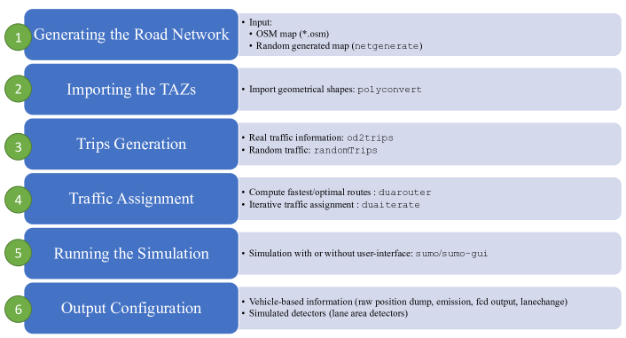
Figure 1: Main steps required to generate and simulate a synthetic traffic scenario with SUMO.

Following, we briefly describe the steps required to generate and simulate a traffic scenario:

• Importing the network: output a road network, generated randomly or extracted from OpenStreetMap;

• Importing the Traffic Analysis Zones (TAZs): import traffic analysis zones definitions. TAZs are polygons that delimitates an urban environment according to some socio-economical indicators (such as average income, education level, traffic pressure, or simply administrative boundaries). TAZs are typically defined by governmental organizations. Dividing the environment into TAZs is useful to model the traffic flow from one local area of a city to another one;

• Trips Generation: for each vehicle, assign origin and destination into the road network. This can be done using real traffic data or randomly;

• Traffic Assignment: model the traffic flow (intended as the set of routes assigned to vehicles). The traffic flow can be generated randomly or starting from OD matrices and using a routing algorithm based on classical methods such as A*;

• Simulation: simulate the traffic model using the defined network and traffic flow;

• Output Configuration: output information generated from the simulation that can be used for traffic analysis purposes;

2.1 Road Network Generation (step ❶)

This section introduces the tools available in SUMO to create a random road network, and to import a road network from OpenStreetMap files.

2.1.1 Random Road Networks

The command netgenerate allows generating three types of abstract road networks: grid (using --grid parameter), spider (using --spider parameter) and random (using --random parameter). The use of randomly generated road networks is pertinent to validate data analysis techniques in traffic domain; the same technique that rely on traffic data can be evaluated on several simulated scenarios, each one having a specific topology, type of junctions, or traffic light options.

The following command creates a random grid-like road network topology:

⬇

> netgenerate --grid --grid.number=10 --grid.length=400

--output-file=MySUMOFile.net.xml

which produces the output shown in Figure 2.

Figure 2: Random grid road network topology generated by netgenerate.

The following command creates a random spider-like road network topology:

⬇

> netgenerate --spider --spider-omit-center --output-file=MySUMOFile.net.xml

which produces the output shown in Figure 3.

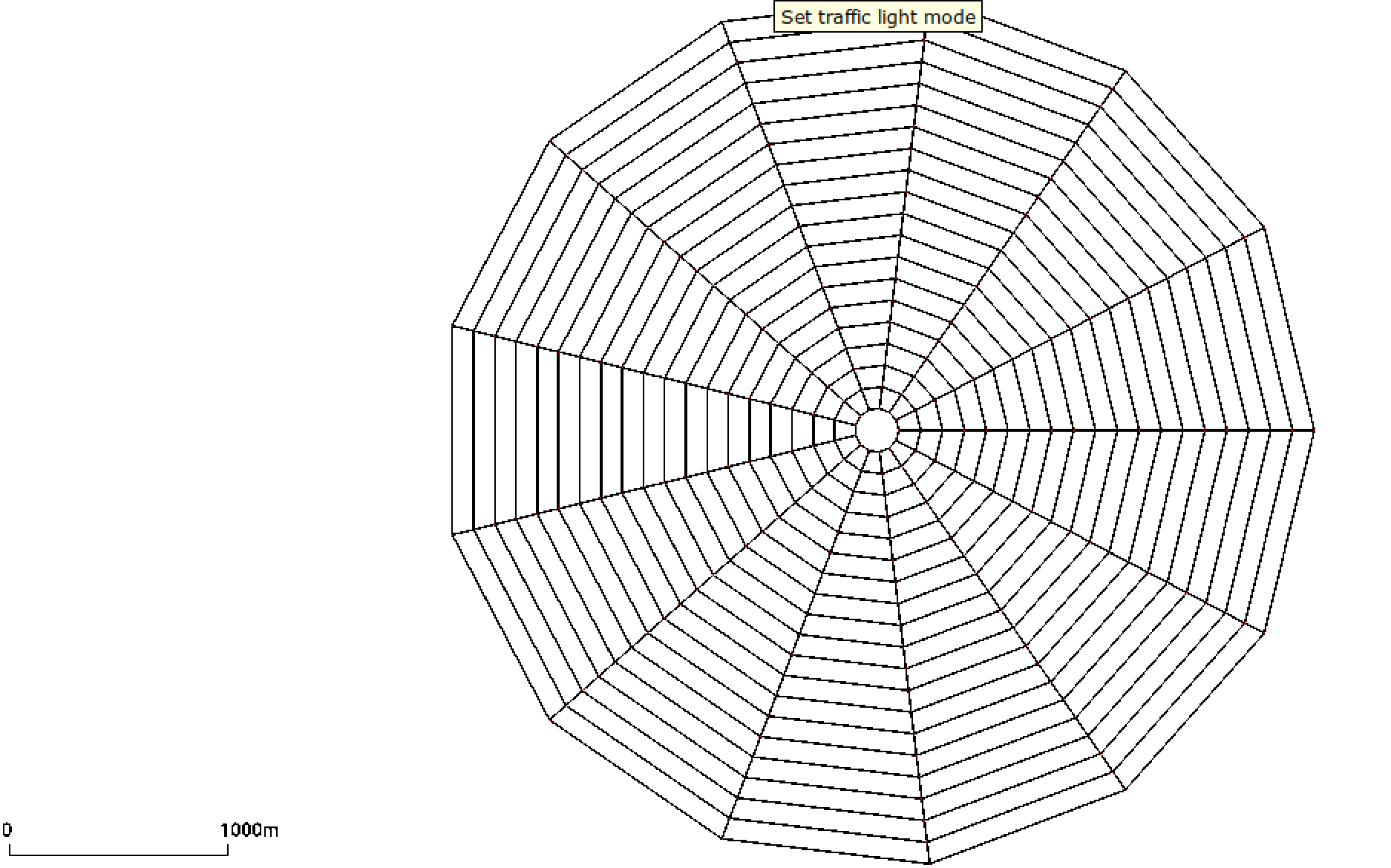
Figure 3: Random spider-like road network topology generated by netgenerate.

The following command creates a random road network topology:

⬇

> netgenerate --rand -o MySUMOFile.net.xml --rand.iterations=200

which produces the output shown in Figure 4.

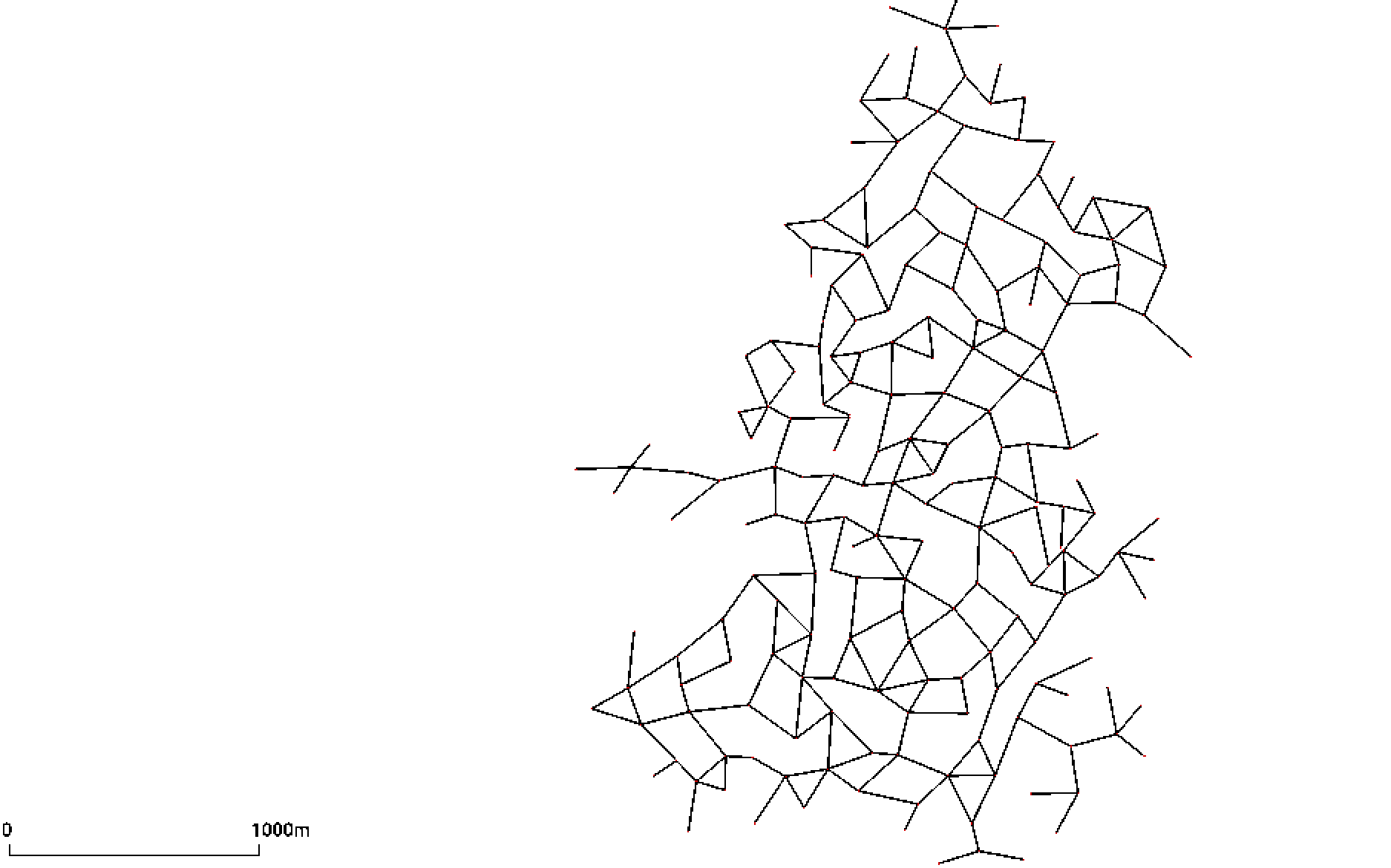
Figure 4: Random road network topology generated by netgenerate.

Additionally, by setting the option --rand.grid, additional grid structure is enforce during random network generation, which produces the output shown in Figure 5.

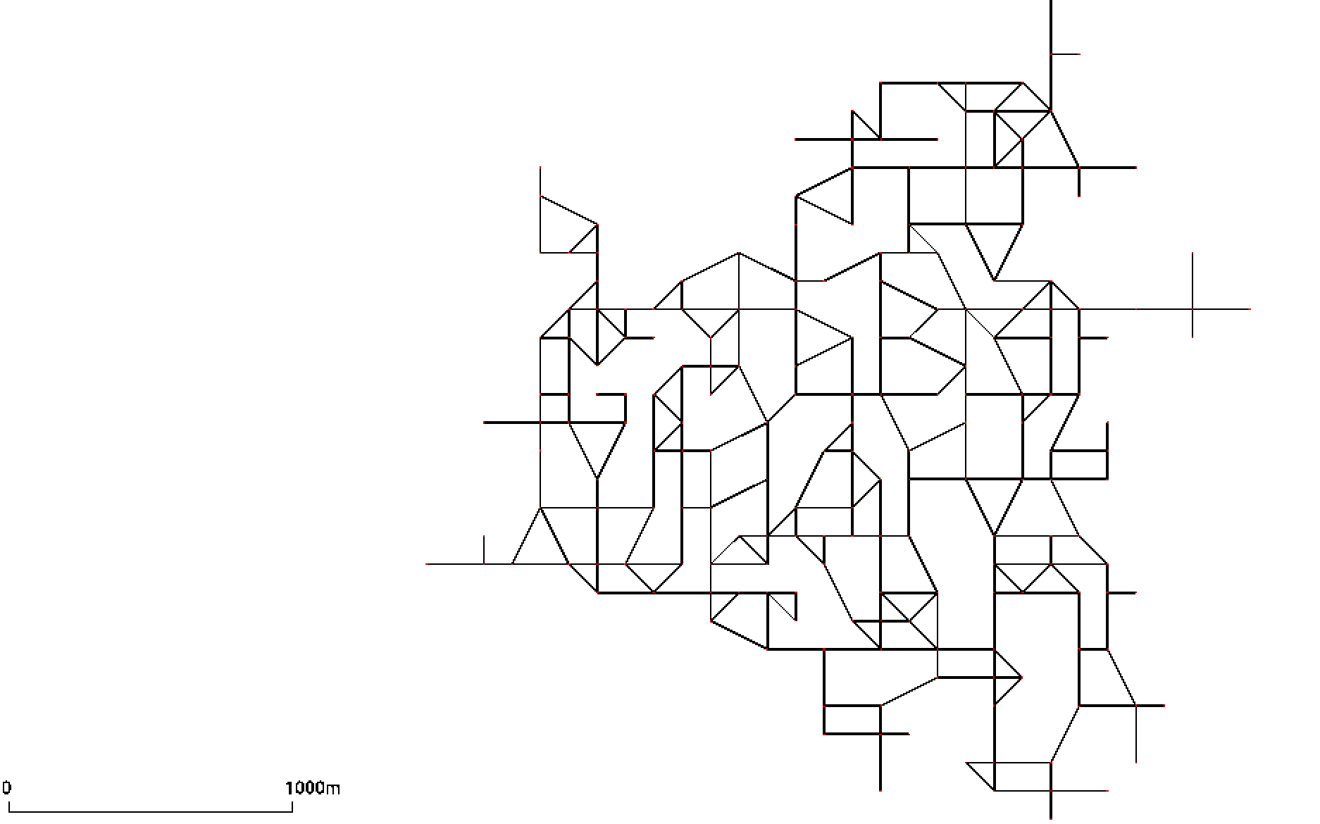
Figure 5:

2.1.2 Extracting a Network Topology from OpenStreetMap

In SUMO, a synthetic model for a real road network can be defined manually. For this, it is necessary to define the XML file that are given in input to SUMO, that include the road network definition, crossroads, traffic lights, etc. This is not feasible when modeling the traffic in a real urban area because of the human effort required to define the road network topology. To tackle this issue, SUMO allows extracting road networks directly from OpenStreetMap (OSM).

The first step to import a road network from OSM in SUMO is to select the region to be modeled, as shown in Figure 6.

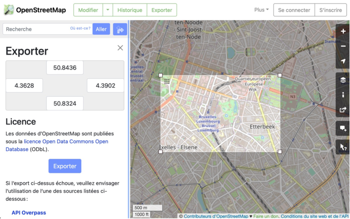
Figure 6: OSM allows exporting a selected area into an XML format.

The next step is to export and download the map. If the “Export” button is selected and the selected area is too big, then OSM will not export the selected area because the number of nodes within the area is above the limit (50000 is the maximum allowed nodes in a selected region for exporting). By selecting the “overpass API” link it is possible to overcome this problem. The output is an XML file containing the definition of all the features in the selected region. In OSM, a feature is any physical element (natural or human-made) in the landscape. Some examples of features are buildings, roads, vegetation, land use, railways, and waterways.

All the features in an OSM XML file are represented as “node” tags. Each node has an identifier, a position (in latitude/longitude), and other useful information that allows identifying the type of node, such as the type of road, building (apartments, offices, theaters, etc.), or bike lane.

To use an OSM map in SUMO, it is necessary to convert the XML file containing the definition of the extracted urban area to a specific format for use with the simulator. To this aim, SUMO comes with a tool named netconvert, that allows importing road networks from different sources. The netconvert  tool can import road networks from the following formats:

• “SUMO plain” XML descriptions (*.edg.xml, *.nod.xml, *.con.xml, *.tll.xml)

• OpenStreetMap (*.osm.xml/*.osm), including shapes (see OpenStreetMap import)

• VISUM, including shapes and demands

• Vissim, including demands

• OpenDRIVE

• MATsim

• SUMO (*.net.xml)

• Shapefiles (.shp, .shx, .dbf), e.g. ArcView and newer Tiger networks

• Robocup Rescue League, including shapes

• a DLR internal variant of Navteq’s GDF (Elmar format)

In its most simple usage, netconvert takes in input only the XML file obtained from OSM (with the parameter --osm), and output a road network (in XML file, using the parameter -o):

⬇

> netconvert --osm my_osm_net.xml -o my_sumo_net.net.xml

2.2 Traffic Assignment Zones (TAZs, step ❷)

A realistic traffic model should describe accurately the traffic dynamics in the urban environment: the traffic flow generated during a simulation of the traffic model is close to that generally found in the real environment corresponding to the simulated environment, and in a specific time horizon. To achieve accuracy in the simulation of a traffic model, it is important to have punctual information about traffic demand, which can be simply defined as the set of all vehicles in a traffic systems, with their associated routes. These information are generally available from city municipalities, and obtained from from sensing devices that are installed into the urban environment, such as induction loops or CCTVs. These devices can provide punctual information about the traffic density in local parts of an urban environment, and enables the definition of usual traffic demand. This information is aggregated over time according to local geographical areas, which are defined according to some socio-economic indicators such as demographic distribution, average income, education level. These local areas are usually defined as Traffic Analysis Zones (TAZs); TAZs are used in traffic demand modeling to represent the spatial distribution of trip origins and destinations, as well as the population, employment and other spatial attributes that generate or otherwise influence travel demand [6]. For instance, Figure 7 shows the TAZs for the city of Bucharest, that are modeled using information on population density, employment density, school population density, road network density [7].

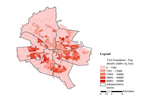
Figure 7: Traffic analysis zones for the city of Bucharest modeled using socio-demographic attributes [7].

Now let us consider the case of the city of Brussels, Belgium. Figure 8 shows the route network of the inner part of the city, extracted from OSM and imported in SUMO using the netconvert tool. The modeled area covers approximately an area of 24.000m². For sake of simplicity, we modeled only the road network, therefore excluding railways and other buildings.

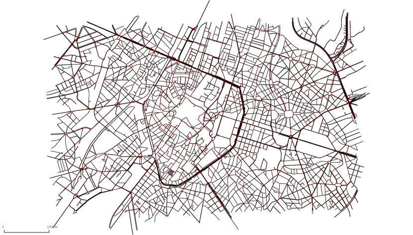
Figure 8: Road network of the city of Brussels.

In this example, we evaluate the TAZs for the modeled area by considering the spatial boundaries of Brussels Capital Region’s neighbourhoods. This data is freely available from the computer center for the Brussels Region (Centre d’Informatique pour la Région Bruxelloise, CIRB). This data is provided as a shapefile, a geo-spatial vector data format commonly used for Geographic Information System (GIS) software.

To use the shapefile in SUMO, this must be converted in a proper format using the polyconvert tool. This can be used to generate all the polygons (e.g., buildings, grounds, etc.) from an input map source (e.g., osm file). Although the output XML file generated from polyconvert is not mandatory to execute a simulation, it is of interest for defining the usual traffic flow between TAZs.

The following command extracts the polygons from a shapefile and write them into the output file bxl.poly.xml. The value “UrbAdm_Monitoring_District” is the prefix of the shapefile from CIRB, containing the spatial boundaries of Brussels neighbourhoods.

⬇

> polyconvert --shapefile-prefix UrbAdm_Monitoring_District

--shapefile.guess-projection true --shapefile.traditional-axis-mapping true

--shapefile.id-column ID -n ../bxl.net.xml -o blx.poly.xml

where UrbAdm_Monitoring_District is the prefix of the shapefile. The parameter --shapefile.guess-projection takes a boolean value: if true, the program guesses the shapefile’s projection. --shapefile.id-column is the name of the column containing the ID of each shape in the shapefile. The parameters -n and -o are respectively the road network definition and the output XML file.

Figure 9 shows the road network of Brussels city and the polygons delimiting the neighborhoods, obtained from the shapefile of CIRB. Each neighborhood is colored randomly. We used the netedit tool to visualize the road network and the neighborhood.

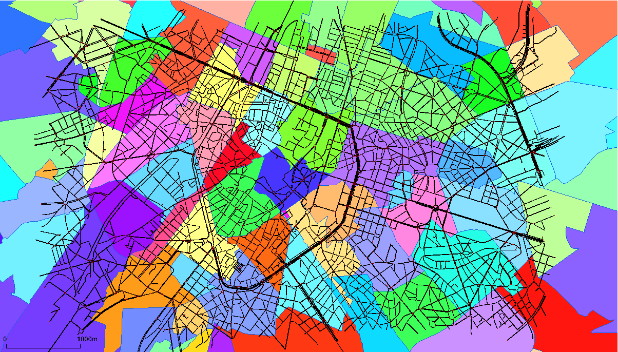
Figure 9: Spatial boundaries of Brussels capital region’s neighborhoods in SUMO. Colors are assigned randomly to each neighborhood.

SUMO provides the tool edgesInDistricts to convert polygons delimiting the neighborhoods in TAZs. This tool reads the polygons from an input file an writes the TAZs to output, including all edges that are located inside the polygons. The following command shows how to use the tool edgesInDistricts:

⬇

> python $SUMO_HOME/tools/edgesInDistricts.py -n bxl.net.xml

-t taz.poly.xml -o TAZ.xml

The output file containing the TAZs has the following format:

⬇

<?xml version="1.0" encoding="UTF-8"?>

<tazs xmlns:xsi="http://www.w3.org/2001/XMLSchema-instance"

xsi:noNamespaceSchemaLocation="http://sumo.dlr.de/xsd/taz_file.xsd">

<taz id="ANDERLECHT CENTRE - WAYEZ" color="51,128,255" edges="-1019451816#0

-1019451816#1 -106463402#0 -106463402#1 ..."/>

<taz id="ANNEESSENS" color="51,128,255" edges="-1007289475 ..."/>

...

</tazs>

In case the polygons that separate the modeled urban area are not available, the TAZs can be generated randomly. SUMO provides two command for this:

• generateBidiDistricts.py: create TAZs and assign to each one edges that are opposite of each other;

• gridDistricts.py: create a grid of TAZs for an input road network, each one with a specified size (in meters).

Figure 10 shows the TAZs generated randomly using the gridDistricts.py tool.

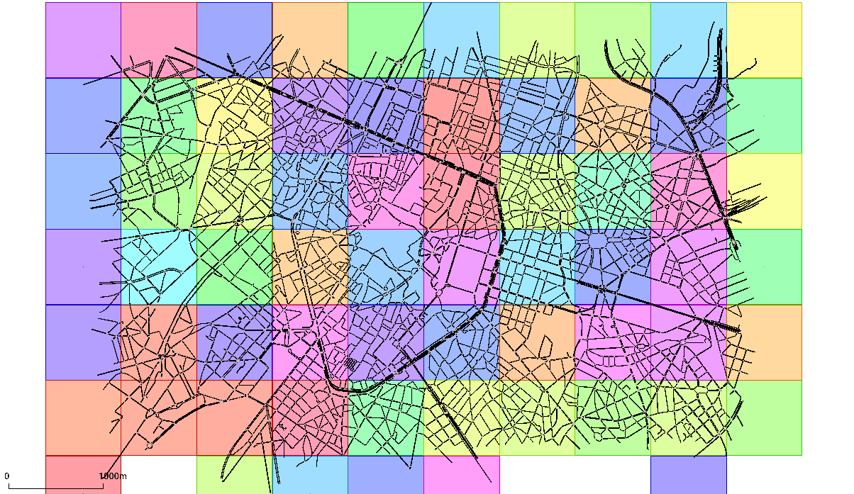
Figure 10: TAZs generated using the gridDistricts.py tool

2.3 Trips Generation (step ❸)

Trips are the building blocks for modeling vehicular traffic flow into a simulation. A trip is identified by a departure time, an origin and a destination point. SUMO includes several tools to model trips starting from realistic socio-economic data, and also to generate synthetic trips.

2.3.1 Importing OD matrices

In traffic demand modeling, the information about traffic flow (trip origins and destinations) is in form of Origin/Destination matrix (shortly OD matrix), where the content of each cell $(i,j)$ indicates the usual density of traffic (that is, the number of vehicles) flowing from TAZ $i$ to TAZ $j$. The resulting matrix is not symmetrical, because during a fixed time interval, the traffic flow between $i$ and $j$ will be different from that between $j$ and $i$. For example, in the OD matrix associated with a given day from 8AM to 9AM, $OD_{ij}$ counts the number of trips from $S_{i}$ to $S_{j}$ during that time interval.

The command od2trips imports OD matrices and splits them into individual vehicle trips. This imports the traffic demand, as a list of origin, destination, and number of vehicles, into an XML output file made of trips; each trip is defined by an id with starting and ending time (included inside the given time-lapse). This command must be run once for each transport mode and for each modeled time horizon. The output is an XML file for the input transport mode and time horizon. The TAZs file is also required as input for this operation.

The following command allows obtaining the trips from file “OD_matrix.od”:

⬇

> od2trips -v --taz-files TAZs.taz.xml --vtype passenger --prefix car

--od-matrix-files OD_matrix.od -o output/output.odtrips.xml

An OD matrix is typically in O-format, that lists each origin and each destination together with the amount of vehicles flowing from origin to destination. Following, we show an example of OD matrix in O-format.

⬇

$OR;D2

* From-Time To-Time

7.00 8.00

* Factor

1.00

1 1 1.00

1 2 2.00

1 3 3.00

2 1 4.00

2 2 5.00

2 3 6.00

3 1 7.00

3 2 8.00

3 3 9.00

where:

• The first line is a format specifier that must be included verbatim.

• The lines starting with ‘*’ are comments and can be omitted

• The second non-comment line determines the time range given as HOUR.MINUTE HOUR.MINUTE

• The third line is a global scaling factor for the number of vehicles for each cell

• All other lines describe matrix cells in the form FROM TO NUMVEHICLES

The tool od2trips outputs an XML file that has the following format:

⬇

<routes xmlns:xsi="http://www.w3.org/2001/XMLSchema-instance"

xsi:noNamespaceSchemaLocation="http://sumo.dlr.de/xsd/routes_file.xsd">

<trip id="0" depart="1.00" from="183370113#1" to="124862958#1"/>

<trip id="1" depart="2.00" from="4441061" to="846162197"/>

<trip id="2" depart="3.00" from="180167843" to="-14858868#1"/>

<trip id="5" depart="8.00" from="4730634#0" to="5451991#0"/>

<trip id="6" depart="8.00" from="41664710#1" to="14858643#0"/>

...

<routes/>

SUMO provides a tool that allows generating OD matrices from TAZs and route files, named route2OD.py. Following, we show how to use this tool, requiring a route file (-r), and a TAZs file (-a).

⬇

> python $SUMO_HOME/tools/route/route2OD.py -r duarouter.rou.xml

-a TAZ.xml -o OD_matrix.xml

2.3.2 Generating Random Trips

SUMO provides the Python script randomTrips.py, that generates a set of random trips for a given road network. It does so by choosing source and destination edge either uniformly at random. The resulting trips are stored in an XML file that can be later used with duarouter, a tool available in SUMO for generating routes. The trips are distributed evenly in a temporal interval defined by begin (option -b, default 0) and end time (option -e, default 3600) in seconds. The number of trips is defined by the repetition rate (option -p, default 1) in seconds.

The following command generates random trips for a given road network (parameter -n):

⬇

> python tools/randomTrips.py -n <net-file> -e 1000

The randomTrips command allows specifying the density of traffic generated per unit of time. By default, one vehicle is added into the simulation at each second. The period at which vehicles are added into the simulation can be specified by using the --period <FLOAT> option: in this way, the arrival rate is of (1/period) per second. By using values below 1, multiple vehicles are added into the simulation at each second.

If several <FLOAT> numbers are provided, like in --period 1.0 0.5, the time interval will be divided equally into subintervals, and the arrival rate for each subinterval is controlled by the corresponding period (in the preceding example, a period of 1.0 will be used for the first subinterval and a period of 0.5 will be used for the second). There are two other ways to specify the insertion rate:

• using the --insertion-rate parameter: this is the number of vehicles per hour that the user expects.

• using the --insertion-density parameter: this is the number of vehicles per hour per kilometer of road that the user expects (the total length of the road is computed with respect to a certain vehicle class that can be changed with the option –edge-permission).

When adding option --binomial <INT> the arrivals will be randomized using a binomial distribution where $n$ (the maximum number of simultaneous arrivals) is given by the argument to --binomial and the expected arrival rate is 1/period.

Let us suppose we want to let n vehicles depart between times t0 and t1 set the options, the following parameters must be provided:

⬇

> python tools/randomTrips.py -n <net-file> -b t0 -e t1 -p ((t1 - t0) / n)

By default the departures of all vehicles are equally spaced in time. Since the inserted vehicle are spread randomly over the whole network, this comes out as a binomial distribution of inserted vehicles for each individual edge which gives a good approximation to the Poisson distribution if the network is large (and hence the insertion probability of each edge is small). By setting set option --random-depart, the (still fixed) number of departure times are drawn from a uniform distribution over [begin, end]. This leads to an exponential distribution of insertion time headways between vehicles on all edges (which is the headway pattern of the Poisson distribution). Hence, this is useful to have a more varied insertion time pattern for small networks.

One interesting feature that is available in randomTrips is that it is possible to assign a unique weight to each edge into the input network by using the --weights-prefix <STRING> paraemter with the prefix value as argument.

The tool will load weights for all edges by finding a file (within the running directory) with extension .src.xml, .dst.xml or .via.xml. According to the file extension, weights are used differently for routes generation:

• .src.xml contains the probabilities for an edge to be selected as from-edge

• .dst.xml contains the probabilities for an edge to be selected as to-edge

• .via.xml contains the probabilities for an edge to be selected as via-edge (only used when option --intermediate is set).

2.4 Traffic Assignment (step ❹)

So far, we described how to create trips, each one containing the origin and the destination of a vehicle, and the time instant in which the vehicle should be inserted in the traffic simulation. Now we explain how to obtain routes. A route contain a list of edges, referring to specific sections of the road network. In other words, a route must be defined for a trip so that the vehicles know how to go from origin to destination.

Vehicular routing in traffic simulation is a relevant problem in the scientific literature: people living in the cities tend to increase the vehicular traffic flow. City road infrastructure does not increase faster than the number of vehicles, thus causing traffic congestion in dense urban centers. In this scenario, maintaining a good vehicular traffic flow has a significant impact on people’s quality of life and even safety. There are several issues related to traffic congestion and, in addition to the impact on the delay, it affects people’s health. The delay also causes the inability to estimate the travel time. Another issue is fuel consumption, which increases due to time wasted on traffic jams [5]. Maintaining a good traffic flow control is a challenging problem because of uncertainties on future traffic dynamics. At the same time, it is equally challenging to design adaptation protocols to handle unexpected events such as accidents or blocked roads: shall only some of the vehicles be routed from one of the alternative routes or all of them? Upon reopening a road segment, shall all vehicles be navigated through that road again? [4].

Although in the scientific literature there are several vehicular routing algorithms [8], herein we will use the routing method provided by SUMO through the duarouter tool. This tool allows the choice between several routing algorithms. By default, Dijkstra is the selected one, but there are other: A*, CH (Contraction Hierarchies), CH Wrapper. The goal of duarouter is to find the shortest path to assign to each vehicle in the simulation. By using the default configuration, duarouter does nothing but calculating the shortest path using Dijkstra’s algorithm and the given edge weights (if provided).

The following command shows how to use the duarouter tool to generate routes:

⬇

> duarouter --net-file osm.net.xml --route-files od2trips.out.xml

--output-file duarouter.rou.xml

where --net-file is the file name of the road network, --route-files it the file containing the trips.

The routing tool can be also used iteratively by the duaIterate.py script. This executes iteratively the following steps, in order:

1. Calling duarouter to perform the re-routing

2. Calling SUMO to simulate travel times

The result of duaIterate.py is an optimized traffic flow. To optimize the flow, the algorithm executes several simulations (the number is a parameter that can be changed). For each simulation, the tool finds a set of routes that reduce the travel time for all vehicles. The algorithm is executed incrementally: at each iteration, it builds a set of routes by considering the routes and the travel time of the last simulation. Two methods can be used when it comes to route choice: Gawron and Logit, both taking a weight/cost function as input.

Gawron proposed a probabilistic approach in which each route choice is modeled by a discrete probability distribution [3]. The algorithm takes in input the following parameters:

• the travel time along the used route in the previous simulation step,

• the sum of edge travel times for a set of alternative routes,

• the probability of choosing a route in the previous simulation step.

In each simulation, a driver $d$ chooses a route $r$ from a set $R_{d}$ (in which the driver is allowed to transit) according to the probability distribution $p_{d}$. Each route is associated with a cost $c_{d}:R_{d}\rightarrow\mathcal{R}_{+}$; this function estimates the time required by the driver to reach the destination. The driver cannot know in advance the amount of traffic in the road network; so, the idea is that the driver evaluate an estimate of the time needed, and updates incrementally (at each simulation) its knowledge about the time required to reach a certain destination.

In Logit method, the required amount of time to travel each road is calculated according to only the information from the last simulation: it ignores old costs and old probabilities and takes the route cost directly as the sum of the edge costs from the last simulation:

$$c^{\prime}_{r}=\sum_{e\in r}w(e)$$ (1)

where $c^{\prime}_{r}$ is the updated cost of route $r$, $w(e)$ is the weight of the edge $e$ calculated from the input weight/cost function. The probability $p^{\prime}_{r}$ for each route $r$ is calculated from an exponential function with parameter $\theta$ scaled by the sum over all route values:

$$p^{\prime}_{r}=\frac{\textnormal{exp}\left(\theta c^{\prime}_{r}\right)}{\sum_{s\in R}\textnormal{exp}\left(\theta c^{\prime}_{s}\right)}$$ (2)

where $c^{\prime}_{r}$ is the cost of route $r$, $w(e)$ is the weight of the edge $e$ calculated from the input weight/cost function.

The following command shows how to use the duaIterate tool to generate optimized routes:

⬇

> python $SUMO_HOME/tools/assign/duaIterate.py -n bxl.net.xml

-t trips.rou.xml -l 2

where -n is the file name of the road network, -t it the file containing the trips, -l the number of iterations (using a number of iterations of 1 is equivalent to calling duarouter).

2.5 Running the simulation (step ❺)

SUMO provide two ways of executing simulations: from the command line (using the sumo command) and from the user interface (using the sumo-gui command). Both command requires several parameters such as the network, the routes, the time horizon over which the simulation must be carried out; another possibility is to provide only one configuration file containing all the parameters required to run a simulation for a specific model, together with the path to the necessary files (network and routes).

⬇

<configuration>

<input>

<net-file value="test.net.xml"/>

<route-files value="test.rou.xml"/>

<additional-files value="test.add.xml"/>

</input>

</configuration>

The simulator can be launched using the following command (assuming that the previous configuration file is named test.sumocfg):

⬇

> sumo -c test.sumocfg

Optionally, SUMO provides a graphical interface, available using the sumo-gui command (instead of sumo). The interface allows for easily monitor traffic flow during the simulation. The interface is customizable so that the user can change the colors and shapes of vehicles and streets. The user interface also allows to:

• watch the simulation, set the delay time to 100, otherwise it runs too fast,

• easily find and view jammed edges,

• set a constant size for the vehicles, and assign them with colors according to various criteria (such as mean speed or waiting time).

Figure 11 shows the sumo user interface.

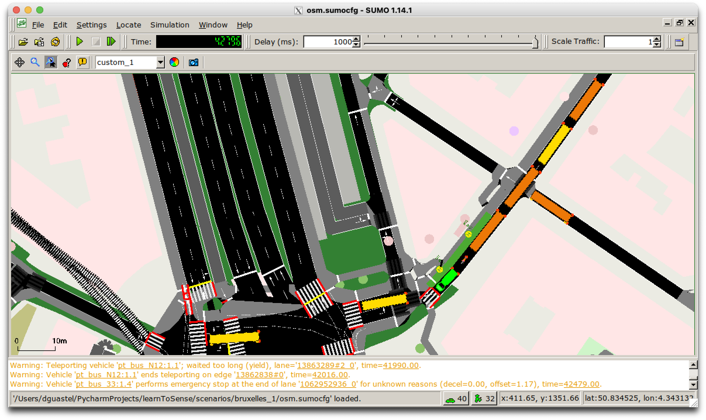
Figure 11: SUMO graphical user interface.

3 Output Configuration (step ❻)

SUMO allows generating output files containing several measures about traffic. These are created as the result of a simulation. Herein we show one method to produce output from simulations. This can be pertinent for use with traffic analysis algorithms. For example, the output data obtained from simulations can be used to analyze traffic pattern or congestion.

A complete list of the output that can be produced by the simulator is available in the SUMO website.

3.1 Using Lane Area Detectors

SUMO enables adding virtual sensors into a road network model to simulate the behavior of CCTVs. These virtual sensors, also known in SUMO as laneAreaDetector, capture traffic on the area along one specific lane. Their functioning is similar to vehicle tracking cameras.

A laneAreaDetector can be added manually using the netedit tool. Figure 12 shows a map of Brussels city where some laneAreaDetector sensors (in teal color) have been placed arbitrarily.

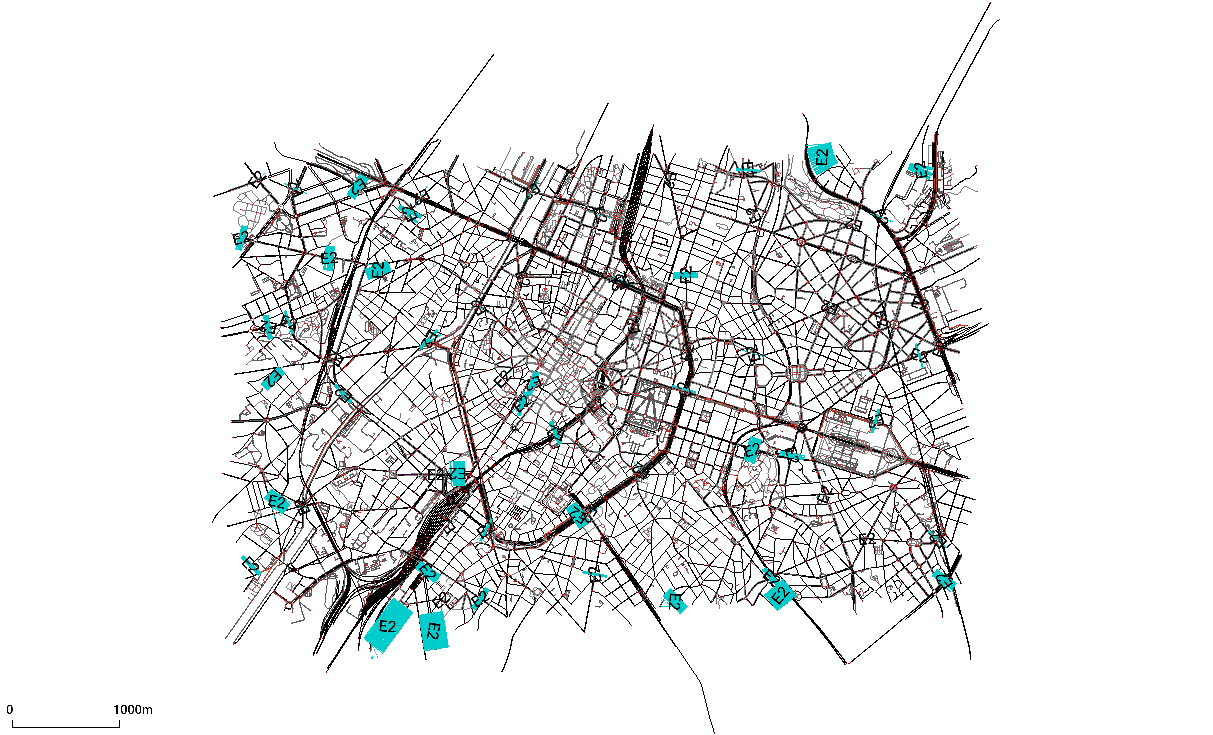
Figure 12: Lane area detectors (virtual sensors) placed into a model of the city of Brussels in SUMO.

From netedit tool, the list of laneAreaDetectors can be exported into an XML file, which has the following format:

⬇

<?xml version="1.0" encoding="UTF-8"?>

<additional xmlns:xsi="http://www.w3.org/2001/XMLSchema-instance"

xsi:noNamespaceSchemaLocation="http://sumo.dlr.de/xsd/additional_file.xsd">

<laneAreaDetector id="e2_0" lane="-159327011#2_0" pos="0.0"

length="138.630000" period="100" file="lane_output/e2_0.xml"/>

<laneAreaDetector id="e2_1" lane="15497309#1_0" pos="0.0"

length="1.940000" period="100" file="lane_output/e2_1.xml"/>

...

</additional>

To use virtual sensors in SUMO, the XML file containing their definition must be provided in input to the simulator. The simulation will write to file the output of the simulated sensors. This includes information such as the number of vehicles observed in an specific time interval, or the mean speed of the observed vehicles.

The path to the XML file containing the definition of laneAreaDetectors must be specified into the <additional> tag, within the sumo configuration file (*.sumocfg), or passed as parameter (-a).

We developed a tool in python language that enables generating and placing laneAreaDetectors randomly in a given road network. The tool performs the following steps, in order:

1. extract the TAZs for the modeled road network (see Section 2.2);

2. extract all the edges and assign them to TAZs;

3. For each TAZ:

   1. choose one random location where to put a laneAreaDetector according to probability $p$;

   2. Place the laneAreaDetectors into the network.

The probability $p$ is calculated according to two strategies:

• by number of lanes: an edge has a probability of getting a virtual sensor proportional to the number of lanes.

• by weight: the probability of an edge of getting a virtual sensor depends on a parameter specified manually, and which values are in the ‘edgedata’ output file produced by SUMO.

When a set of laneAreaDetectors is provided to SUMO, the simulator outputs several XML files (one per virtual sensor) containing, among the others, the information listed in Table 1. The output file for each virtual sensor is specified in the field file in the tag <laneAreaDetector>.

Table 1: Subset of data types returned by each laneAreaDetector at the end of a simulation.

Name	Unit	Description
begin	(simulation) seconds	The first time step the values were collected in
end	(simulation) seconds	The last time step + DELTA_T the values were collected in (may be equal to begin)
id	id	The id of the detector (needed if several detectors share an output file)
meanSpeed	m/s	The mean velocity over all collected data samples.
meanTimeLoss	s	The average time loss per vehicle in the corresponding interval. The total time loss can be obtained by multiplying this value with nVehSeen.
meanOccupancy	%	The percentage (0-100%) of the detector’s place that was occupied by vehicles, summed up for each time step and averaged by the interval duration.
maxOccupancy	%	The maximum percentage (0-100%) of the detector’s place that was occupied by vehicles during the interval.
maxVehicleNumber	#	The maximum number of vehicles that were on the detector area during the interval.

4 Tools for the Automatic Definition of Scenarios

4.1 SUMO OSM Web Wizard

The OSM Web Wizard is a web-based tool that offers an easy solutions to start modeling traffic scenarios with SUMO. The user can specify the area to model graphically through an openstreetmap map excerpt, and configure a randomized traffic demand and run and visualize the scenario in the sumo-gui. To run this tool, the following command must be run:

⬇

> python $SUMO_HOME/tools/osmWebWizard.py

Figure 13 shows the OSM Web Wizard interface.

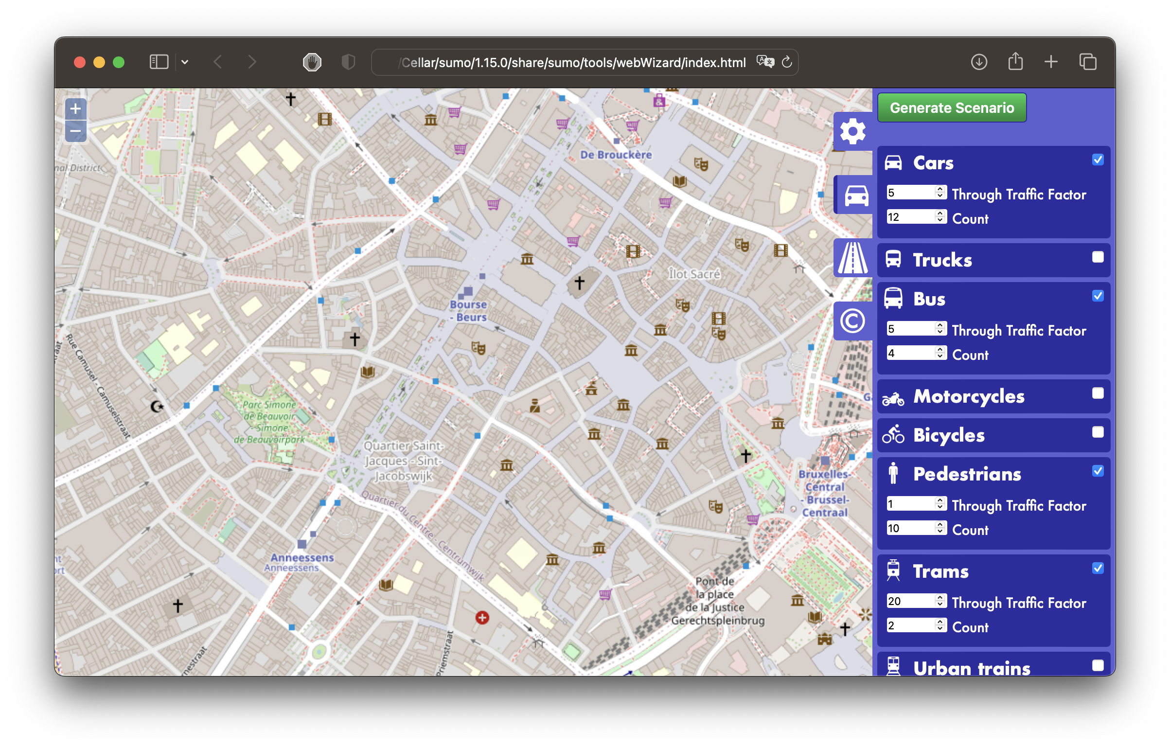
Figure 13: SUMO OSM Web Wizard user interface.

4.2 SAGA

SUMO Activity GenerAtion (SAGA) is a user-defined activity-based multimodal mobility scenario generator for SUMO [1]. SAGA is capable of handling activity-based mobility from detailed information on the environment (e.g., buildings, PoIs), as well as the transportation infrastructure. SAGA is capable of extracting environmental information available automatically (from OSM) such as building and public transportation lines, generating all the configuration files required by SUMO, and fills the missing information with sensible default values. The output scenario is multi-modal, that is, including different types of transportation mean for population, and includes also parking areas, buildings, Points of Interest (PoIs).

Appendix A Full Step-by-Step Examples

A.1 Example 1

Step 1 – Network generation

⬇

netgenerate --rand -o MySUMOFile.net.xml --rand.iterations=200

-j traffic_light --random

Step 2 – Random trips generation

⬇

python $SUMO_HOME/tools/randomTrips.py -n MySUMOFile.net.xml -e 3600

-o trips.rou.xml --random

Step 3 – Routing

⬇

duarouter --net-file MySUMOFile.net.xml --route-files trips.rou.xml

--output-file duarouter.rou.xml --ignore-errors

Step 4 – Configuration file generation

⬇

echo "<configuration>

<input>

<net-file value=\"MySUMOFile.net.xml\"/>

<route-files value=\"duarouter.rou.xml\"/>

</input>

</configuration>" | tee -a sumo.sumocfg

Step 5 – Simulation

⬇

sumo-gui -c sumo.sumocfg

A.2 Example 2

Step 1 – Network generation

⬇

netgenerate --rand -o MySUMOFile.net.xml --rand.iterations=300

-j traffic_light --random --rand.grid

Step 2 – Random trips generation

⬇

python $SUMO_HOME/tools/randomTrips.py -n MySUMOFile.net.xml -e 3600

-o trips.rou.xml --random --random-depart --binomial 20

Step 3 – Routing

⬇

duarouter --net-file MySUMOFile.net.xml --route-files trips.rou.xml

--output-file duarouter.rou.xml --ignore-errors --route-choice-method logit

Step 4 – Configuration file generation

⬇

echo "<configuration>

<input>

<net-file value=\"MySUMOFile.net.xml\"/>

<route-files value=\"duarouter.rou.xml\"/>

</input>

</configuration>" tee -a sumo2.sumocfg

Step 5 – Simulation

⬇

sumo-gui -c sumo2.sumocfg

A.3 Example 3

Step 1 – Get the map from OSM

⬇

python $SUMO_HOME/tools/osmGet.py --bbox="4.3583, 50.8362, 4.3696, 50.8455"

Step 2 – OSM map to SUMO network

⬇

python $SUMO_HOME/tools/osmBuild.py --osm-file osm_bbox.osm.xml

Step 3 – Extract the polygons from the OSM file

⬇

polyconvert --net-file osm.net.xml --osm-files osm_bbox.osm.xml

--type-file $SUMO_HOME/share/sumo/data/typemap/osmPolyconvert.typ.xml

-o polygons.poly.xml

Step 4 – Generate random trips

⬇

python $SUMO_HOME/tools/randomTrips.py -n osm.net.xml -e 3600 -o trips.rou.xml

--random --random-depart --binomial 10 --validate

Step 5 – Routing

⬇

duarouter --net-file osm.net.xml --route-files trips.rou.xml

--output-file duarouter.rou.xml --ignore-errors true

Step 6 – Configuration file generation

⬇

echo "<configuration>

<input>

<net-file value=\"osm.net.xml\"/>

<route-files value=\"duarouter.rou.xml\"/>

<additional-files value=\"polygons.poly.xml\"/>

</input>

</configuration>" tee -a sumo.sumocfg

Step 7 – Simulation

⬇

sumo-gui -c sumo2.sumocfg

A.4 Example 4

Step 1 – Scenario Definition

⬇

python $SUMO_HOME/tools/osmGet.py --bbox="4.3583, 50.8362, 4.3696, 50.8455"

python $SUMO_HOME/tools/osmBuild.py --osm-file osm_bbox.osm.xml

Step 2 – TAZs Extraction

⬇

polyconvert --net-file osm.net.xml --osm-files osm_bbox.osm.xml

--type-file $SUMO_HOME/share/sumo/data/typemap/osmPolyconvert.typ.xml

-o polygons.taz.xml --type taz

python $SUMO_HOME/tools/edgesInDistricts.py

-n osm.net.xml -t polygons.taz.xml -o TAZ.xml

-l passenger --complete

Step 3 – Random Traffic Generation

⬇

python $SUMO_HOME/tools/randomTrips.py -n osm.net.xml

-b 0 -e 3600 -o trips.rou.xml --random --random-depart

--binomial 10 --validate

Step 4 – Random traffic to OD-matrix

⬇

python $SUMO_HOME/tools/route/route2OD.py

-r trips.rou.xml -a TAZ.xml -o routes.xml -i 5

Step 5 – Importing OD-matrix

⬇

od2trips -z routes.xml -n TAZ.xml -b 0 -e 3600

-o od2trips.out.xml

Step 6 – Routing and Simulation

⬇

duarouter --net-file osm.net.xml --route-files od2trips.out.xml

--output-file duarouter.rou.xml --ignore-errors true

sumo-gui +a TAZ.xml -n osm.net.xml -r od2trips.out.xml -b 0

-e 3600 --edgedata-output edgedata.outsampler.xml --ignore-route-errors

A.5 Example 5

This example shows how to generate an inter-modal traffic scenario. We assume that the file “map.osm” is the map downloaded from OSM.

Step 1 – OSM to SUMO, Public Transportation Data Extraction

⬇

netconvert --osm-files map.osm -o bxl.net.xml --osm.stop-output.length 20

--ptstop-output additional.xml --ptline-output ptlines.xml

Step 2 – Find Travel Times and Create Public Transportation Schedules

⬇

python $SUMO_HOME/tools/ptlines2flows.py -n bxl.net.xml -s additional.xml

-l ptlines.xml -o flows.rou.xml -p 600 --use-osm-routes --ignore-errors

Step 3 – Generate Random Traffic for Vehicles

⬇

python $SUMO_HOME/tools/randomTrips.py -n bxl.net.xml -b 0 -e 3600

-o passenger_trips.rou.xml --random --random-depart --validate

--vehicle-class passenger

Step 4 – Vehicles Routing

⬇

duarouter --net-file bxl.net.xml --route-files passenger_trips.rou.xml

--output-file duarouter_passenger.rou.xml --ignore-errors

Step 5 – Simulation

⬇

sumo-gui -n bxl.net.xml -r duarouter_passenger.rou.xml,flows.rou.xml -b 0

-e 3600 --edgedata-output edgedata.outsampler.xml

-a additional.xml --ignore-route-errors

Appendix B SUMO Installation

Detailed installation instructions are available in the SUMO website: https://sumo.dlr.de/docs/Installing/index.html

For OSX, we suggest using Homebrew (https://brew.sh/) to install SUMO. We recommend to use the following commands, in order:

⬇

> brew install --cask xquartz

> brew tap dlr-ts/sumo

> brew install --with-examples --with-ffmpeg

--with-gdal --with-gl2ps --with-swig sumo

After the installation, the system variable SUMO_HOME must be set (system-wide) to the path containing SUMO. Typically the path is as the following: /opt/homebrew/Cellar/sumo/1.XX.XX/.

Appendix C Common Issues

C.1 Broken Folder Links When Using SUMO on OSX

When using SUMO installed through homebrew into the path /opt/homebrew/Cellar/sumo/1.XX.XX/, the following commands must be run to fix broken links in SUMO folders:

⬇

sudo ln -s $SUMO_HOME/share/sumo/tools/ $SUMO_HOME/

sudo ln -s $SUMO_HOME/share/sumo/data $SUMO_HOME/

4 Useful Resources

• https://www.eltis.org/sites/default/files/tool/conduits_key_performance_indicators_its.pdf

• https://www.arcgis.com/home/item.html?id=f40c3fdb26c74e64af4f2cb8311c5559

• https://monitoringdesquartiers.brussels/maps/statistiques-population-bruxelles/evolution-population/densite-de-population/1/2019/#

• https://www.acea.auto/files/ACEA-report-vehicles-in-use-europe-2022.pdf

• Number of households with cars (Belgium): https://statbel.fgov.be/en/themes/datalab/vehicles-household

References

- [1] L. Codeca, J. Erdmann, V. Cahill, and J. Haerri. SAGA: An Activity-based Multi-modal Mobility ScenarioGenerator for SUMO. SUMO Conference Proceedings, 1:39–58, June 2022.
- [2] S. Dorokhin, A. Artemov, D. Likhachev, A. Novikov, and E. Starkov. Traffic simulation: an analytical review. IOP Conference Series: Materials Science and Engineering, 918(1):012058, September 2020.
- [3] C. Gawron. An Iterative Algorithm to Determine the Dynamic User Equilibrium in a Traffic Simulation Model. International Journal of Modern Physics C, 09(03):393–407, May 1998.
- [4] I. Gerostathopoulos and E. Pournaras. TRAPPed in Traffic? A Self-Adaptive Framework for Decentralized Traffic Optimization. In 2019 IEEE/ACM 14th International Symposium on Software Engineering for Adaptive and Self-Managing Systems (SEAMS), pages 32–38, Montreal, QC, Canada, May 2019. IEEE.
- [5] D. L. Guidoni, G. Maia, F. S. H. Souza, L. A. Villas, and A. A. F. Loureiro. Vehicular Traffic Management Based on Traffic Engineering for Vehicular Ad Hoc Networks. IEEE Access, 8:45167–45183, 2020.
- [6] E. J. Miller. Traffic analysis zone definition: issues & guidance. 2021.
- [7] S. Raicu, D. Costescu, and S. Burciu. Analysis of intrinsic factors contributing to urban road crashes. International Journal of Safety and Security Engineering, 7(1):1–9, 2017.
- [8] V. Tran Ngoc Nha, D. Soufiene, and J. Murphy. A comparative study of vehicles’ routing algorithms for route planning in smart cities. In 2012 First International Workshop on Vehicular Traffic Management for Smart Cities (VTM), pages 1–6, 2012.