Neural Attention Forests: Transformer-Based Forest Improvement

Abstract

A new approach called NAF (the Neural Attention Forest) for solving regression and classification tasks under tabular training data is proposed. The main idea behind the proposed NAF model is to introduce the attention mechanism into the random forest by assigning attention weights calculated by neural networks of a specific form to data in leaves of decision trees and to the random forest itself in the framework of the Nadaraya-Watson kernel regression. In contrast to the available models like the attention-based random forest, the attention weights and the Nadaraya-Watson regression are represented in the form of neural networks whose weights can be regarded as trainable parameters. The first part of neural networks with shared weights is trained for all trees and computes attention weights of data in leaves. The second part aggregates outputs of the tree networks and aims to minimize the difference between the random forest prediction and the truth target value from a training set. The neural network is trained in an end-to-end manner. The combination of the random forest and neural networks implementing the attention mechanism forms a transformer for enhancing the forest predictions. Numerical experiments with real datasets illustrate the proposed method. The code implementing the approach is publicly available.

1 Introduction

The attention mechanism can be viewed as an approach for the crucial improvement of neural networks in recent years. It is based on weighing features or examples in accordance with their importance to enhance the machine learning model accuracy. Successful applications of the attention mechanism to many important tasks, including natural language processing, computer vision, etc., motivated a large interest to developing various attention-based models [2, 5, 6, 13, 14]. Most attention-based models are implemented as components of neural networks such that the attention weights are learned within the neural architectures. In order to avoid several problems inherent in neural networks, such as overfitting, lack of sufficient data, etc. and to use the attention mechanism without neural networks, an attention-based random forests (ABRF) and some its extensions have been proposed in [10, 15]. Several ideas behind the ABRF were presented. The first one is to use random forests (RFs) [3] as an ensemble-based model which effectively deals with tabular data. The problem is that neural networks successfully process various types of data, including images, text data, graphs. However, they are inferior to many simple models, for example, RFs, gradient boosting machines, when they are dealing with tabular data. The second idea behind the ABRF is to apply the well-known Nadaraya-Watson (N-W) kernel regression [12, 17] which learns a non-linear function by using a weighted average of the data where weights are nothing else but the attention weights [4, 18]. The third idea is to assign trainable weights to decision trees in the RF depending on examples, which fall into leaves of trees, and their features. The weights are trained by solving a simple quadratic optimization problem which is constructed as a standard loss function to minimize the classification or regression errors. The ABRF have demonstrated outperforming results on many real datasets. In spite of the ABRF efficiency, these models use the standard Gaussian kernels with trainable parameters to train the attention weights. Moreover, the set of trainable attention parameters is rather narrow and does not allow us to significantly enhance the predicted accuracy of the model.

In order to overcome the above difficulties, we propose to combine the RF and the neural network of a specific architecture. Actually, the neural network implements a set of attention operations and consists of two parts. The first part of neural networks with shared weights is trained for all trees and computes attention weights of data in leaves. The second part aggregates outputs of the “tree” networks and aims to minimize the difference between the random forest prediction and the truth target value from a training set. These parts are jointly trained in an end-to-end manner. The combination of the random forest and neural networks implementing the attention mechanism forms a transformer for enhancing the forest predictions.

Our contributions can be summarized as follows. A new Neural Attention Forest architecture called as NAF is proposed to overcome difficulties of RFs and neural networks when we deal with tabular data. The attention mechanism is implemented by two different parts of the neural network. The first part computes trainable attention weights depending on trees and examples. The second part of the network aggregates weighted outputs of trees. Numerical experiments with real datasets are performed for studying NAF. They demonstrate outperforming results of NAF in comparison with RFs. The code of proposed algorithms can be found at https://github.com/andruekonst/NAF.

The paper is organized as follows. A brief introduction to the attention mechanism as the N-W kernel regression and the attention-based random forest is given in Section 2. A general architecture of NAF is considered in Section 3. The transformer implementation of NAF is provided in Section 4. Numerical experiments with real data illustrating properties of NAF are provided in Section 5. Concluding remarks can be found in Section 6.

2 Preliminaries

2.1 Nadaraya-Watson regression and attention

Suppose that a dataset $\mathcal{D}$ is represented by $n$ examples $(\mathbf{x}_{1},y_{1}),...,(\mathbf{x}_{n},y_{n})$, where $\mathbf{x}_{i}=(x_{i1},...,x_{id})\in\mathbb{R}^{d}$ is a feature vector; $y_{i}\in\mathbb{R}$ is a regression output. The regression task is to construct a regressor $f:\mathbb{R}^{d}\rightarrow\mathbb{R}$ which can predict the output value $\widehat{y}$ of a new observation $\mathbf{x}$, using the dataset. The N-W kernel regression model [12, 17] is one of the methods to estimate the function $f$ by applying the weighted averaging as follows:

$$\widehat{y}=\sum_{i=1}^{n}\alpha(\mathbf{x},\mathbf{x}_{i})y_{i},$$ (1)

where weight $\alpha(\mathbf{x},\mathbf{x}_{i})$ conforms with relevance of the feature vector $\mathbf{x}_{i}$ to the vector $\mathbf{x}$, i.e., the closer $\mathbf{x}_{i}$ to $\mathbf{x}$, the greater the weight $\alpha(\mathbf{x},\mathbf{x}_{i})$ assigned to $y_{i}$.

Weights are calculated by using a normalized kernel $K(\mathbf{x},\mathbf{x}_{i})$ as:

$$\alpha(\mathbf{x},\mathbf{x}_{i})=\frac{K(\mathbf{x},\mathbf{x}_{i})}{\sum_{j=1}^{n}K(\mathbf{x},\mathbf{x}_{j})}.$$ (2)

According to [1], vector $\mathbf{x}$, vectors $\mathbf{x}_{i}$, outputs $y_{i}$, and weight $\alpha(\mathbf{x},\mathbf{x}_{i})$ are called as the query, keys, values, and the attention weight, respectively. Weights $\alpha(\mathbf{x},\mathbf{x}_{i})$ can be extended by incorporating trainable parameters. Several types of attention weights have been proposed in literature. The most important examples are the additive attention [1], multiplicative or dot-product attention [11, 16].

2.2 Attention-based random forest

A powerful machine learning model handling tabular data is the RF which is represented as an ensemble of $T$ trees such that each tree is trained on a subset of examples randomly selected from the training set. A prediction $\widehat{y}$ for a new example $\mathbf{x}$ in the RF is determined by averaging predictions $\widehat{y}_{1},...,\widehat{y}_{T}$ obtained for all trees in the RF. Let us denote an index set of examples, which jointly with $\mathbf{x}$ fall into the same leaf in the $k$-th tree, as $\mathcal{J}_{k}(\mathbf{x})$. Then the corresponding leaf can be characterized by the vector $\mathbf{A}_{k}(\mathbf{x)}$ which is the mean of all $\mathbf{x}_{j}$ from $\mathcal{D}$ such that $j\in\mathcal{J}_{k}(\mathbf{x})$, and the vector $B_{k}(\mathbf{x)}$ which is a mean of all $y_{j}$ from $\mathcal{D}$ by $j\in\mathcal{J}_{k}(\mathbf{x})$. According to ABRF [15], the N-W regression can be rewritten in terms of the RF as:

$$\widehat{y}=\sum_{k=1}^{T}\alpha\left(\mathbf{x},\mathbf{A}_{k}(\mathbf{x)},\theta\right)\cdot B_{k}(\mathbf{x)},$$ (3)

where $\theta$ is a vector of training attention parameters.

It follows from definitions of the attention mechanism that $B_{k}(\mathbf{x)}$, $\mathbf{A}_{k}(\mathbf{x)}$, and $\mathbf{x}$ are the value, the key, and the query, respectively. If to return to the original RF, then all its trees have the same weights $\alpha\left(\mathbf{x},\mathbf{A}_{k}(\mathbf{x)},\theta\right)=1/T$. Parameters $\theta$ are trained by minimizing the expected loss function $L$ over a set $\Theta$ of parameters as follows:

$$\theta_{opt}=\arg\min_{\theta\mathbf{\in}\Theta}~{}\sum_{s=1}^{n}L\left(\widehat{y}_{s},y_{s},\theta\right),$$ (4)

where $\widehat{y}_{s}$, $y_{s}$ are the truth target value and the predicted output of the $s$-th input example, respectively.

The original ABRF uses the Gaussian kernel for computing the attention weights and the Huber’s $\epsilon$-contamination model [9] to reduce the problem (4) to the standard quadratic optimization problem with linear constraints. However, the obtained approach cannot cover a wide range of possible kernels and models for computing $\mathbf{A}_{k}(\mathbf{x)}$, $B_{k}(\mathbf{x)}$ and other parameters. Moreover, the set of trainable parameters $\theta$ in the ABRF is also restrictive. Therefore, we propose a general approach which uses neural networks to compute the attention weights simultaneously with $\mathbf{A}_{k}(\mathbf{x)}$ and $B_{k}(\mathbf{x)}$ such that the neural network weights are trainable attention parameters $\theta$.

3 The neural attention forest architecture

A general NAF architecture is shown in Fig.1. Suppose that we have built a RF consisting of $T$ decision trees on the training set $\mathcal{D}$. A feature vector $\mathbf{x}$ is fed to each tree, and the path of $\mathbf{x}$ to a leaf is depicted by the red line. Several feature vectors $\mathbf{x}_{j}$ as well as the corresponding output values $y_{j}$ fall into the same leaf with $j\in\mathcal{J}_{k}(\mathbf{x})$. The first part of the neural network (Att in Fig.1) implementing the attention mechanism is represented by $T$ networks with shared weights $\theta$ (parameters of the networks). It can be seen from Fig.1 that the $k$-th neural network implements the attention operation and computes vector $\mathbf{A}_{k}(\mathbf{x)}$ and value $B_{k}(\mathbf{x)}$ in accordance with the N-W regression as follows:

$$\mathbf{A}_{k}(\mathbf{x)}=\sum_{j\in\mathcal{J}_{k}(\mathbf{x})}\alpha\left(\mathbf{x},\mathbf{x}_{j},\theta\right)\mathbf{x}_{j},$$ (5)

$$B_{k}(\mathbf{x)}=\sum_{j\in\mathcal{J}_{k}(\mathbf{x})}\alpha\left(\mathbf{x},\mathbf{x}_{j},\theta\right)y_{j}.$$ (6)

where $\alpha\left(\mathbf{x},\mathbf{x}_{j},\theta\right)$ is the attention weight having trainable parameters $\theta$ (parameters of the networks) and is defined by the following scaled dot-product score function [11]: $\alpha(\mathbf{x},\mathbf{x}_{j})=\mathbf{x}^{T}\mathbf{x}_{j}\mathbf{/}\sqrt{d}$.

In sum, we get keys $\mathbf{A}_{k}(\mathbf{x)}$ and values $B_{k}(\mathbf{x)}$ for all trees. The second part of the neural network is the global attention (GAtt in Fig.1) which aggregates all keys $\mathbf{A}_{k}(\mathbf{x)}$ and values $B_{k}(\mathbf{x)}$ in accordance with the N-W regression as follows:

$$\widehat{\mathbf{x}}=\sum_{k=1}^{T}\beta\left(\mathbf{x},\mathbf{A}_{k}(\mathbf{x)},\psi\right)\cdot\mathbf{A}_{k}(\mathbf{x)},$$ (7)

$$\widehat{y}=\sum_{k=1}^{T}\beta\left(\mathbf{x},\mathbf{A}_{k}(\mathbf{x)},\psi\right)\cdot B_{k}(\mathbf{x)},$$ (8)

where $\beta$ is the attention weight with parameters $\psi$ (parameters of the second part of the network).

Note that the accurately trained NAF predicts vector $\widehat{\mathbf{x}}$ which should be close to $\mathbf{x}$. By comparing $\widehat{\mathbf{x}}$ and $\mathbf{x}$, we can judge the quality of training the network and the RF. NAF is learned in an end-to-end manner by using the loss function

$$(\theta,\psi)_{opt}=\arg\min_{\theta,\psi}~{}\sum_{s=1}^{n}\left(\widehat{y}_{s}-y_{s}\right)^{2}.$$ (9)

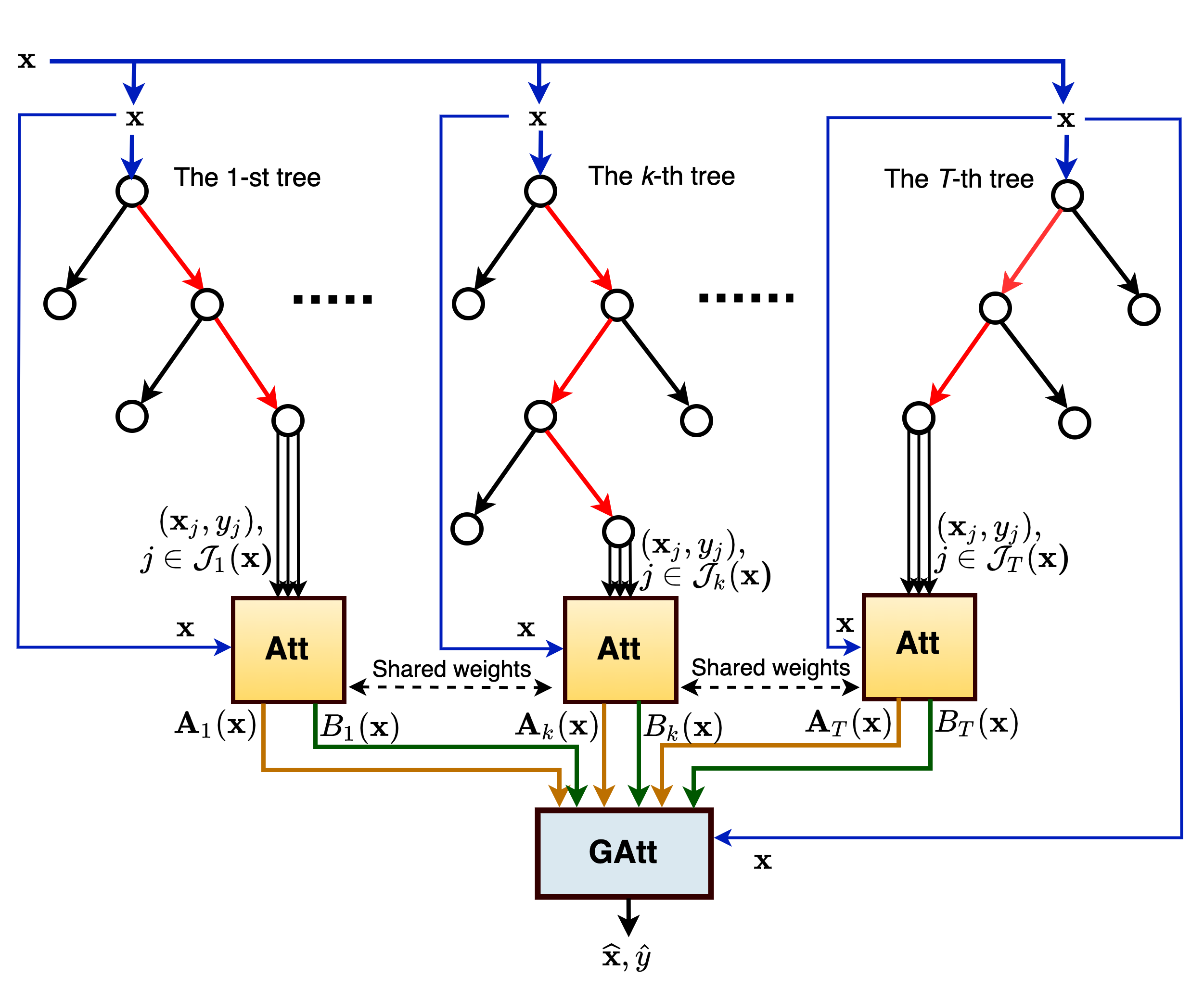
Figure 1: The neural attention forest architecture

4 The neural attention forest as a transformer

Let us represent the set of examples $(\mathbf{x}_{j},y_{j})$, $j\in\mathcal{J}_{k}(\mathbf{x})$, which fall jointly with the feature vector $\mathbf{x}$ in the same $p$-th leaf of the $k$-th tree, as a sentence $\mathbf{s}$ consisting of words denoted as $w_{i}^{(k,p)}$, $i\in\mathcal{J}_{k}(\mathbf{x})$, i.e.,

$$\mathbf{s}_{k,p}=\left\{w_{i_{1}}^{(k,p)},...,w_{i_{r}}^{(k,p)}\right\}.$$ (10)

Here $r$ is the number of elements in $\mathcal{J}_{k}(\mathbf{x})$; $k$ is the number of a tree; $p$ is the number of the leaf; $i$ is the example index (the word index in the $p$-th sentence), which falls into the $p$-th leaf. Sentences $\mathbf{s}_{k,t}$ and $\mathbf{s}_{l,p}$ produced by the $t$-th and the $p$-th trees and consisting of $3$ and $2$ words, respectively, as an illustrative example are shown in Fig.2.

The above implies that every leaf produces a sentence $\mathbf{s}_{k,p}$. In sum, we have a set $\mathcal{S}$ of sentences $s$ produced by all leaves. Query $\mathbf{x}$ can also be regarded as a word $\overline{w}=(\mathbf{x})$ which consists of $\mathbf{x}$ and does not contain $y$ that has to be estimated.

Let us construct a model

$$\mathcal{M}_{\theta}\left(\mathbf{s}_{k,p},\overline{w}\right)=\mathcal{M}_{\theta}\left(w_{i_{1}}^{(k,p)},...,w_{i_{r}}^{(k,p)};\overline{w}\right).$$ (11)

The above notation means that $\overline{w}$ is the query, $w_{i_{1}}^{(k,p)},...,w_{i_{r}}^{(k,p)}$ are pairs of keys $\mathbf{x}_{j}$ and values $y_{j}$, $j\in\mathcal{J}_{k}(\mathbf{x})$, in the attention model. In other words, we compute $\mathbf{A}_{k}(\mathbf{x)}$ and $B_{k}(\mathbf{x)}$ by using $\mathcal{M}_{\theta}\left(\mathbf{s}_{k,p};\overline{w}\right)$ in accordance with (5) and (6).

Denote the set of all words defined by the training set $\mathcal{D}$ as $\mathcal{W}$. If we consider only the level of the first neural networks, then an optimization problem for learning parameters $\theta$ of $\mathcal{M}_{\theta}$ can be written as

$$\sum_{w\in\mathcal{W}}\sum_{\mathbf{s}\in\mathcal{S}:w\in\mathbf{s}}\left\|\mathcal{M}_{\theta}\left(\mathbf{s}\backslash w;\overline{w}\right)-w\right\|^{2}\rightarrow\min_{\theta}.$$ (12)

However, the second part of the neural network should be taken into account. Therefore, we have to aggregate the models $\mathcal{M}_{\theta}$ obtained for all trees. Let us return to the attention operations (7) and (7). Then the loss function can be rewritten as

$$\sum_{w\in\mathcal{W}}\left\|Q\left(\widehat{w}-w\right)\right\|^{2}=\sum_{w\in\mathcal{W}}\left\|Q\left(\sum_{t=1}^{T}\beta\left(\widetilde{w}_{t}\right)\cdot\widetilde{w}_{t}-w\right)\right\|^{2},$$ (13)

where $\widetilde{w}_{t}$ is defined as

$$\widetilde{w}_{t}=\mathcal{M}_{\theta}\left(\mathbf{s}^{(t)}(w)\backslash w;\overline{w}\right),$$

$\mathbf{s}^{(t)}(\overline{w})$ is a sentence produced by the $t$-th tree, which contains the word $w$ (there exists exactly one such sentence); $Q$ is a $(d+1)\times(d+1)$ diagonal matrix whose diagonal is $(\lambda_{1},\lambda_{2},...,\lambda_{d},1)$; $0\leq\lambda_{i}\leq 1$ is the hyperparameter which determines the weight of the $i$-th feature in the loss function, the last $1$ in the diagonal of matrix $Q$ indicates that $y$ from the word $w$ and $\widehat{y}$ from $\widehat{w}$ have to be used.

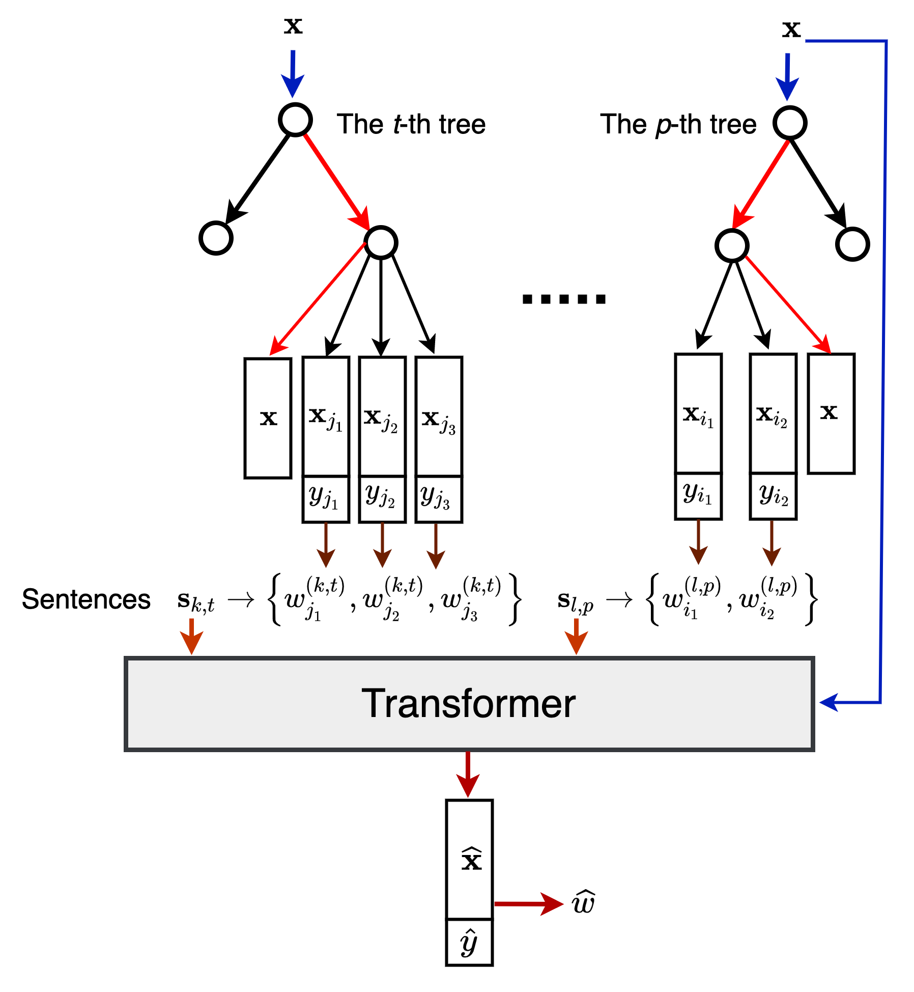
Figure 2: A scheme how sentences for the transformer are produced by trees

5 Numerical experiments

In order to study NAF, we build two types of the forests. The first one is the original RF. The second forest is the Extremely Randomized Trees (ERT) proposed by Geurts et al. [8]. In contrast to RFs, the ERT algorithm at each node chooses a split point randomly for each feature and then selects the best split among these features.

In all experiments, RFs as well as ERTs consist of $100$ trees. A 3-fold cross-validation on the training set consisting of $n_{\text{tr}}=4n/5$ examples with $100$ repetitions is performed. The testing set for computing the accuracy measures consists of $n_{\text{test}}=n/5$ examples. In order to get desirable estimates of vectors $\mathbf{A}_{k}(\mathbf{x})$ and values $B_{k}(\mathbf{x})$, all trees in experiments are trained such that at least $10$ examples fall into every leaf of a tree. The coefficient of determination denoted as $R^{2}$ is used for the regression evaluation. The greater the value of the coefficient of determination, the better results we get.

NAF is investigated by applying datasets which are taken from open sources. The dataset Diabetes is downloaded from the R Packages; datasets Friedman 1, 2, 3, Regression and Sparse are taken from package “Scikit-Learn”; datasets Boston Housing (Boston) and Yacht Hydrodynamics (Yacht) can be found in the UCI Machine Learning Repository [7].

Values of the measure $R^{2}$ for several models, including RF, ERT, NAF with one layer having 16 units and linear activations added by the softmax operation (NAF-1), and NAF with three layers having 16 units in two layers with the tanh activation function and one linear layer (NAF-3) are shown in Table 1 which also contain a brief information about the datasets (the number of features $m$ and the number of examples $n$). Results presented in Table 1 are given for two cases when the RF and the ERT are used. The best results separately for NAFs based on the RF and the ERT are shown in bold. It should be pointed out that NAF demonstrates outperforming results for most dataset. Moreover, one can see from Table 1 that NAF based on the ERT provides better results in comparison the NAF based on the RF. A very important comment with respect to the obtained results is that we have used the simplest neural network having one layer (NAF-1). Even this simple network has ensured the outperforming results.

Table 1: Values of $R^{2}$ for comparison of models based on the RF and the ERT

			RF			ERT
Data set	$m$	$n$	Original	NAF-1	NAF-3	Original	NAF-1	NAF-3
Diabetes	$10$	$442$	$0.417$	$0.382$	$\mathbf{0.418}$	$0.438$	$0.396$	$\mathbf{0.442}$
Friedman 1	$10$	$100$	$0.459$	$\mathbf{0.506}$	$0.487$	$0.471$	$0.514$	$\mathbf{0.530}$
Friedman 2	$4$	$100$	$0.840$	$\mathbf{0.903}$	$0.892$	$0.813$	$\mathbf{0.943}$	$0.921$
Friedman 3	$4$	$100$	$0.625$	$\mathbf{0.720}$	$0.635$	$0.570$	$\mathbf{0.608}$	$0.578$
Boston	$13$	$506$	$0.814$	$\mathbf{0.846}$	$0.832$	$0.831$	$\mathbf{0.857}$	$0.855$
Yacht	$6$	$308$	$0.981$	$0.976$	$\mathbf{0.985}$	$0.988$	$\mathbf{0.995}$	$0.992$
Regression	$100$	$100$	$\mathbf{0.380}$	$0.291$	$0.346$	$0.402$	$0.333$	$\mathbf{0.406}$
Sparse	$10$	$100$	$0.470$	$\mathbf{0.671}$	$0.613$	$0.452$	$\mathbf{0.701}$	$0.665$

One of the advantages of NAF is its simple example-based explanation which selects instances of the dataset to explain the prediction. The idea behind the explanation is to use the property of NAF to predict (or reconstruct) $\widehat{\mathbf{x}}$ which is close to input vector $\mathbf{x}$. If the reconstructed vector $\widehat{\mathbf{x}}$ is actually close to the input vector $\mathbf{x}$, then the nearest neighbors for the reconstructed vector can be regarded as examples explaining a prediction. For the explanation experiments, we build 500 trees of the ERT on the well-known “two moons” dataset. Moreover, we use a condition that at least $1$ example falls into every leaf of a tree. $25$ points are taken for training. The measure $R^{2}$ is $0.781$ for the ERT, and is $0.936$ for NAF. Fig.3 illustrates results provided by three models: the original ERT (the left picture), the random NAF with random weights of the neural network (the middle picture), and NAF-1 (the right picture). First, it can be seen from the middle picture that the reconstructed vector depicted by the small square is far from the input vector depicted by the small star because the network with random weights provides incorrect results. Therefore, the neighbors of $\widehat{\mathbf{x}}$ cannot be viewed as examples for explanation. However, it can be seen from the right picture in Fig.3 that NAF provides the reconstructed vector which is close to the input vector. Therefore, its nearest neighbors can be used for the example-based explanation. The nearest neighbors are also defined by their weight (the small circle size) calculated as product of two attention weights $\alpha\left(\mathbf{x},\mathbf{A}_{k}(\mathbf{x)},\theta\right)$ and $\beta\left(\mathbf{x},\mathbf{A}_{k}(\mathbf{x)},\psi\right)$.

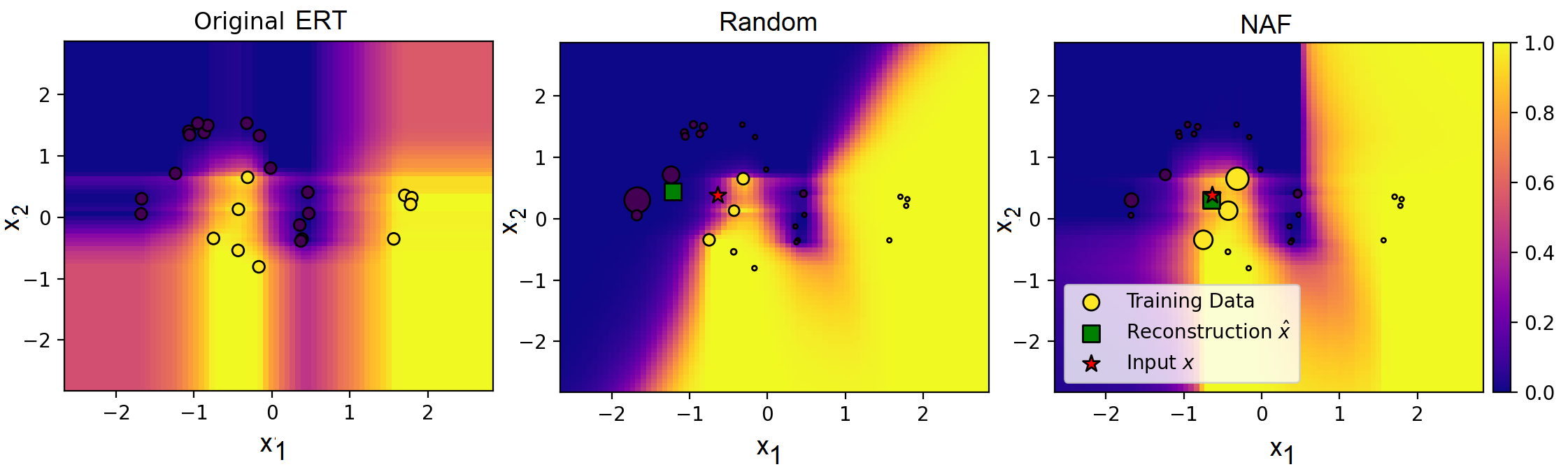
Figure 3: Illustration of the example-based explanation on the “two moons” dataset

6 Concluding remarks

A new approach to combining RFs and attention-based neural networks for solving regression and classification tasks under tabular training data has been proposed. It has been shown that the proposed model can be represented as a transformer-based model which improves the RF. Numerical experiments with real datasets have demonstrated that NAF provides outperforming results even when simple one-layer neural networks are used to implement the attention operations.

NAF opens a door for developing a new class of neural attention forest models and a new class of transformers. One of the interesting directions for further research is to consider the attention when different RFs are built with the same data. Moreover, this idea leads to implementation of the multi-head attention and the cross-attention depending on a scheme of training the corresponding RFs. Another direction for research is to consider the NAF as an autoencoder which transforms the input vector $\mathbf{x}$ into its estimates $\widehat{\mathbf{x}}$. By using this representation, we can construct a new anomaly detection procedure under condition of small data. It should be noted that NAF can also be a basis for developing a weakly supervised model. First, we learn trees by using a small labeled dataset. Then we learn the neural network on unlabeled data minimizing the difference between reconstructed vector $\widehat{\mathbf{x}}$ and the input vector $\mathbf{x}$ as a loss function. Then the unlabeled examples can be regarded as new tested examples, and their labels can be estimated by NAF. This is a perspective direction for research.

The above directions is a part of many improvements and modifications of NAF, which could significantly extend the class of the neural attention forest models.

References

- [1] Bahdanau, D., Cho, K., Bengio, Y.: Neural machine translation by jointly learning to align and translate (Sep 2014), arXiv:1409.0473
- [2] Brauwers, G., Frasincar, F.: A general survey on attention mechanisms in deep learning. IEEE Transactions on Knowledge and Data Engineering (2021)
- [3] Breiman, L.: Random forests. Machine learning 45(1), 5–32 (2001)
- [4] Chaudhari, S., Mithal, V., Polatkan, G., Ramanath, R.: An attentive survey of attention models (Apr 2019), arXiv:1904.02874
- [5] Chaudhari, S., Mithal, V., Polatkan, G., Ramanath, R.: An attentive survey of attention models. ACM Transactions on Intelligent Systems and Technology 12(5), 1–32 (2021), article 53
- [6] Correia, A., Colombini, E.: Attention, please! A survey of neural attention models in deep learning. Artificial Intelligence Review 55(8), 6037–6124 (2022)
- [7] Dua, D., Graff, C.: UCI machine learning repository (2017), http://archive.ics.uci.edu/ml
- [8] Geurts, P., Ernst, D., Wehenkel, L.: Extremely randomized trees. Machine learning 63, 3–42 (2006)
- [9] Huber, P.: Robust Statistics. Wiley, New York (1981)
- [10] Konstantinov, A., Utkin, L., Kirpichenko, S.: AGBoost: Attention-based modification of gradient boosting machine. In: 31st Conference of Open Innovations Association (FRUCT). pp. 96–101. IEEE (2022). https://doi.org/10.23919/FRUCT54823.2022.9770928
- [11] Luong, T., Pham, H., Manning, C.: Effective approaches to attention-based neural machine translation. In: Proceedings of the 2015 Conference on Empirical Methods in Natural Language Processing. pp. 1412–1421. The Association for Computational Linguistics (2015)
- [12] Nadaraya, E.: On estimating regression. Theory of Probability & Its Applications 9(1), 141–142 (1964)
- [13] Niu, Z., Zhong, G., Yu, H.: A review on the attention mechanism of deep learning. Neurocomputing 452, 48–62 (2021)
- [14] Tay, Y., Dehghani, M., Bahri, D., Metzler, D.: Efficient transformers: A survey. ACM Computing Surveys 55(6), 1–28 (2022)
- [15] Utkin, L., Konstantinov, A.: Attention-based random forest and contamination model. Neural Networks 154, 346–359 (2022)
- [16] Vaswani, A., Shazeer, N., Parmar, N., Uszkoreit, J., Jones, L., Gomez, A., Kaiser, L., Polosukhin, I.: Attention is all you need. In: Advances in Neural Information Processing Systems. pp. 5998–6008 (2017)
- [17] Watson, G.: Smooth regression analysis. Sankhya: The Indian Journal of Statistics, Series A pp. 359–372 (1964)
- [18] Zhang, A., Lipton, Z., Li, M., Smola, A.: Dive into deep learning. arXiv:2106.11342 (Jun 2021)