Indirect imprints of primordial non-Gaussianity on cosmic microwave background

Abstract

Primordial non-Gaussianity arising from inflationary models is a unique probe of non-trivial dynamics of the inflaton field and its interactions with other fields. Often when examining and constraining the scalar non-Gaussianity arising from inflation, certain templates are adopted for the scalar non-Gaussianity parameter $f_{{}_{\rm NL}}$, in classifying their behaviors in terms of wavenumbers. The current constraints from cosmic microwave background (CMB) on such templates of $f_{{}_{\rm NL}}$ are weak and provide rather large bounds on their amplitudes. In this work, we explore a different method of constraining $f_{{}_{\rm NL}}$ through their effect on the scalar power. We compute the correction to the scalar power due to $f_{{}_{\rm NL}}$ while accounting for its generic scale dependence. We then compute the angular power spectrum of CMB arising from such non-Gaussian corrections to explore possible imprints. We initially illustrate this method using the conventional templates of $f_{{}_{\rm NL}}$ such as local, equilateral and orthogonal types, with and without the running of the parameter. We further employ this method to an oscillatory form of $f_{{}_{\rm NL}}$ and lastly on a realistic model of inflation proposed by Starobinsky. Though this method does not improve much on the constraints on the first three templates of $f_{{}_{\rm NL}}$, it provides interesting insights on models that do not conform to these templates. We infer that the non-Gaussian correction to the spectrum can be sensitive to model parameters that are degenerate at the level of the original power spectrum. Hence, this method of computing indirect imprints of $f_{{}_{\rm NL}}$ on angular power spectrum of CMB provides a new avenue to explore primordial scalar non-Gaussianity and possibly constrain them effectively.

I Introduction

Models of inflation that give rise to a variety of non-trivial features in the primordial scalar power spectrum have been studied widely in the literature (for some of the earlier efforts, refer [1, 2, 3, 4], and for recent efforts, see [5, 6, 7]). They are sought for their promise of improvement in the fit to the data of anisotropies in the cosmic microwave background at the level of angular power spectrum [8, 9]. Such features arise primarily due to non-trivial dynamics of the evolution of the inflaton field, in the context of canonical single field inflationary models. These models also give rise to scalar non-Gaussianities of large amplitudes and non-trivial shapes and they have been explored at the level of bispectrum [10, 11, 12, 13, 14, 15, 16, 17].

While features at the level of power spectrum have been well constrained against CMB dataset, the constraints are relatively weaker at the level of bispectrum. The scalar non-Gaussianity parameter associated with the bispectrum, $f_{{}_{\rm NL}}$, is typically parametrized using certain well-motivated templates, called local, equilateral and orthogonal templates, which are supposed to represent broad classes of models [18, 19, 20, 21]. These templates provide ease of comparison against data and the current constraints on the amplitudes of $f_{{}_{\rm NL}}$ of the respective templates are $f_{{}_{\rm NL}}^{\rm loc}=-0.9\pm 5.1$, $f_{{}_{\rm NL}}^{\rm eq}=-26\pm 47$ and $f_{{}_{\rm NL}}^{\rm ortho}=-38\pm 24$ at $1-\sigma$ level [22]. These large bounds, obtained with the current level of sensitivity of the Planck mission, certainly rule out exotic models of inflation leading to large non-Gaussianity but do not inform much about the typical models and the associated parameters that govern the scalar bispectrum. Moreover, we should note that these simple templates are not sufficient to describe the non-trivial shapes of $f_{{}_{\rm NL}}$ that arise in models that lead to features in the power spectrum. Hence, it is challenging to compare the exact shape and behavior of $f_{{}_{\rm NL}}$ arising out of realistic models of inflation directly against data and obtain constraints on the model parameters determining the scalar non-Gaussianity.

In the absence of data and analysis techniques with better constraining power, we explore a method to examine $f_{{}_{\rm NL}}$ through its indirect effect on the angular power spectrum of CMB. We calculate the non-Gaussian correction to the primordial scalar power spectrum due to $f_{{}_{\rm NL}}$ [23, 24]. Further, we compute the corresponding CMB angular spectrum and compare it against the original spectrum due to Gaussian perturbations. An important advantage of this method is that, it accounts for the complete and arbitrary scale dependence of $f_{{}_{\rm NL}}$ without relying on templates. Also, it is computationally simpler than a direct of comparison of $f_{{}_{\rm NL}}$ against data. Therefore, it is robust enough to be employed for any given model of inflation and arrive at possibly better bounds on $f_{{}_{\rm NL}}$ and the relevant model parameters.

This approach is equivalent to computing the one-loop correction to the spectrum when the modes of perturbations are unaffected in the super-Hubble regime, which is especially true for the large scales of CMB. There have been several efforts in the context of computing loop-corrections to primordial spectrum [25, 26, 27, 28, 29]. We should also note that there is considerable interest in recent literature in computing such loop-level non-Gaussian contributions to the scalar power, especially in the context of enhancing scalar power over small scales in ultra slow roll models of inflation [23, 30, 31, 32, 33, 34, 35]. Such loop corrections have interesting implications for the case of primordial perturbations evolving from excited initial states [24, 36]. There are also efforts to study loop-level contribution to the spectrum of $21$ cm signal [37], and to the spectral density of scalar-induced secondary gravitational waves [38, 39, 40, 41, 42, 43]. In this work, we utilize this method to compute possible imprints of $f_{{}_{\rm NL}}$ on the angular spectrum of CMB and study the possibility of effectively constraining the relevant model parameters.

The article is organized as follows. In Sec. II, we outline the computational scheme to calculate the correction to the scalar power due to $f_{{}_{\rm NL}}$. In Sec. III, we illustrate our method using the typical templates of $f_{{}_{\rm NL}}$, with and without a running that may be present in these templates. We also employ it on an oscillatory template of $f_{{}_{\rm NL}}$ which gives us more insight into spectra with non-trivial scale dependences. In Sec. IV, we employ the method to a realistic model of inflation that was originally proposed by Starobinsky. Lastly, we conclude with a summary and outlook in Sec. V.

As to the notations used in the article, we denote the original scalar power spectrum as $\mathcal{P}_{{}_{\mathrm{S}}}(k)$ and the non-Gaussian correction to the spectrum as $\mathcal{P}_{{}_{\mathrm{C}}}(k)$. We use $f_{{}_{\rm NL}}(k_{1},k_{2},k_{3})$ to denote the complete form of the scalar non-Gaussianity parameter, while denote the amplitudes of parameter in specific templates as $f_{{}_{\rm NL}}^{\rm type}$, where ‘${\rm type}$’ may be ${\rm loc}$, eq, ${\rm ortho}$ or ${\rm osc}$, denoting the respective templates.

II Correction to the power spectrum due to $f_{{}_{\rm NL}}(k_{1},k_{2},k_{3})$

In this section, we shall setup the method of calculating the correction to the primordial scalar power spectrum arising due to $f_{{}_{\rm NL}}(k_{1},k_{2},k_{3})$. We shall briefly outline the detailed derivation as presented in Ref. [42] and also closely follow the conventions therein. We consider the mode function associated with the primordial curvature perturbation, namely ${\mathcal{R}}_{\bm{k}}$ and expand it in Fourier space to include the related non-Gaussianity as

$${\mathcal{R}}_{\bm{k}}(\eta) = {\mathcal{R}}^{{}^{{}_{\rm G}}}_{\bm{k}}(\eta)-\frac{3}{5}\int\frac{{\mathrm{d}}^{3}{\bm{k}}_{1}}{(2\,\pi)^{3/2}}{\mathcal{R}}^{{}^{{}_{\rm G}}}_{\bm{k_{1}}}(\eta){\mathcal{R}}^{{}^{{}_{\rm G}}}_{\bm{k}-\bm{k_{1}}}(\eta)\,f_{{}_{\rm NL}}[\bm{k},({\bm{k}}_{1}-\bm{k}),-{\bm{k}}_{1}]\,,$$ (1)

where $\eta$ denotes the conformal time and ${\mathcal{R}}^{{}^{{}_{\rm G}}}_{\bm{k}}$ denotes the Gaussian part of ${\mathcal{R}}_{\bm{k}}$. Such an expansion has been used in different contexts in literature [44, 45]. This expansion generalizes the conventional expansion of curvature perturbation in real space as ${\mathcal{R}}(\bm{x},\eta)={\mathcal{R}}^{{}^{{}_{\rm G}}}(\bm{x},\eta)-(3/5)f_{{}_{\rm NL}}[{\mathcal{R}}^{{}^{{}_{\rm G}}}(\bm{x},\eta)]^{2}\,,$ where $f_{{}_{\rm NL}}$ is assumed to be local without any scale-dependence (see, for instance, Refs. [46, 11]). We are interested in computing ${\mathcal{R}}_{\bm{k}}(\eta)$ at $\eta_{\rm e}$ close to the end of inflation. There can be additional time dependence in this expansion through$f_{{}_{\rm NL}}$. But for the large scales of our interest, the modes at $\eta_{\rm e}$ are in their super-Hubble regime. Even if there are brief departures from slow-roll during inflation, as long as there is a slow-roll phase prior to the end of inflation, these modes are largely unaffected and are essentially constant in their amplitudes. Therefore, the time dependence in $f_{{}_{\rm NL}}$ due to deviations from slow-roll between Hubble-exit of modes and $\eta_{e}$ shall be negligible.

To illustrate that $f_{{}_{\rm NL}}(k_{1},k_{2},k_{3})$ captures the non-Gaussianity arising from the scalar bispectrum, we can compute the two-point and three-point correlations of ${\mathcal{R}}_{\bm{k}}(\eta)$ as expanded in Eq. (1). Using the definitions of scalar power and bi-spectra, $\mathcal{P}_{{}_{\mathrm{S}}}(k)$ and ${\cal B}(k_{1},k_{2},k_{3})$ [46]

$$\langle{\mathcal{R}}^{{}^{{}_{\rm G}}}_{{\bm{k}}_{1}}{\mathcal{R}}^{{}^{{}_{\rm G}}}_{{\bm{k}}_{2}}\rangle = \frac{2\pi^{2}}{k_{1}^{3}}\mathcal{P}_{{}_{\mathrm{S}}}(k_{1})\delta^{(3)}({\bm{k}}_{1}+{\bm{k}}_{2})\,,$$ (2)

$$\langle{\mathcal{R}}^{{}^{{}_{\rm G}}}_{{\bm{k}}_{1}}{\mathcal{R}}^{{}^{{}_{\rm G}}}_{{\bm{k}}_{2}}{\mathcal{R}}^{{}^{{}_{\rm G}}}_{{\bm{k}}_{3}}\rangle = (2\pi)^{3}\,{\cal B}(k_{1},k_{2},k_{3})\delta^{(3)}({\bm{k}}_{1}+{\bm{k}}_{2}+{\bm{k}}_{3})\,,$$ (3)

we can show that the non-Gaussianity parameter $f_{{}_{\rm NL}}(k_{1},k_{2},k_{3})$ can be expressed in terms of them as [11, 13, 5, 42, 17]

$$f_{{}_{\rm NL}}(k_{1},k_{2},k_{3}) = -\frac{10\sqrt{(2\pi)}}{3}\frac{(k_{1}k_{2}k_{3})^{3}{\cal B}(k_{1},k_{2},k_{3})}{\bigg{[}k_{1}^{3}\mathcal{P}_{{}_{\mathrm{S}}}(k_{2})\mathcal{P}_{{}_{\mathrm{S}}}(k_{3})+k_{2}^{3}\mathcal{P}_{{}_{\mathrm{S}}}(k_{1})\mathcal{P}_{{}_{\mathrm{S}}}(k_{3})+k_{3}^{3}\mathcal{P}_{{}_{\mathrm{S}}}(k_{1})\mathcal{P}_{{}_{\mathrm{S}}}(k_{2})\bigg{]}}\,.$$ (4)

The expectation values in the definitions used above are evaluated in the perturbative vacuum typically at $\eta_{e}$. As we see, $f_{{}_{\rm NL}}(k_{1},k_{2},k_{3})$ is a dimensionless ratio of bispectrum to combination of power spectra. It is proportional to the scalar bispectrum ${\cal B}(k_{1},k_{2},k_{3})$ that receives its dominant contributions from the cubic order action governing ${\mathcal{R}}_{\bm{k}}(\eta)$. Therefore $f_{{}_{\rm NL}}(k_{1},k_{2},k_{3})$ captures the non-Gaussianity due to three-point auto-correlation of ${\mathcal{R}}_{\bm{k}}(\eta)$.

To compute the correction to the power spectrum $\mathcal{P}_{{}_{\mathrm{C}}}(k)$ due to $f_{{}_{\rm NL}}(k_{1},k_{2},k_{3})$, we compute the two point correlation of $\hat{\mathcal{R}}_{k}(\eta)$ of Eq. (1) as

$$\langle\hat{{\mathcal{R}}}_{\bm{k_{1}}}\hat{{\mathcal{R}}}_{\bm{k_{2}}}\rangle = \langle\hat{\cal R}^{{}^{{}_{\rm G}}}_{\bm{k_{1}}}\hat{\cal R}^{{}^{{}_{\rm G}}}_{\bm{k_{2}}}\rangle+\frac{9}{25}\int\frac{{\mathrm{d}}^{3}{\bm{k}}_{1}^{\prime}}{(2\,\pi)^{3}}\int{\mathrm{d}}^{3}{\bm{k}}_{2}^{\prime}\langle\hat{\cal R}^{{}^{{}_{\rm G}}}_{\bm{k^{\prime}_{1}}}\hat{\cal R}^{{}^{{}_{\rm G}}}_{\bm{k_{1}}-\bm{k^{\prime}_{1}}}\hat{\cal R}^{{}^{{}_{\rm G}}}_{\bm{k^{\prime}_{2}}}\hat{\cal R}^{{}^{{}_{\rm G}}}_{\bm{k_{2}}-\bm{k^{\prime}_{2}}}\rangle$$ (5)

$$\times\,f_{{}_{\rm NL}}\big{(}k_{1},|{\bm{k}}_{1}^{\prime}-{\bm{k}}_{1}|,k_{1}^{\prime}\big{)}\,f_{{}_{\rm NL}}\big{(}k_{2},|{\bm{k}}_{2}^{\prime}-{\bm{k}}_{2}|,k_{2}^{\prime}\big{)}\,.$$

Using Wick’s theorem to express the four point correlation in terms of the two point correlations, the above equation becomes

$$\mathcal{P}_{{}_{\mathrm{S}}}^{\rm M}(k) = \mathcal{P}_{{}_{\mathrm{S}}}(k)+\frac{9}{50\pi}k^{3}\int{\mathrm{d}}^{3}{\bm{k}}_{1}\,\frac{\mathcal{P}_{{}_{\mathrm{S}}}(k_{1})}{k_{1}^{3}}\frac{\mathcal{P}_{{}_{\mathrm{S}}}(|\bm{k}-{\bm{k}}_{1}|)}{|\bm{k}-{\bm{k}}_{1}|^{3}}\,f_{{}_{\rm NL}}^{2}[k,|{\bm{k}}_{1}-\bm{k}|,k_{1}]\,,$$ (6)

where $\mathcal{P}_{{}_{\mathrm{S}}}(k)$ denotes the original power spectrum corresponding to the Gaussian perturbations ${\mathcal{R}}^{{}^{{}_{\rm G}}}_{\bm{k}}(\eta)$, $\mathcal{P}_{{}_{\mathrm{S}}}^{\rm M}(k)$ is the complete modified spectrum and the correction $\mathcal{P}_{{}_{\mathrm{C}}}(k)$ can be identified as

$$\mathcal{P}_{{}_{\mathrm{C}}}(k) = \frac{9}{50\pi}k^{3}\int{\mathrm{d}}^{3}{\bm{k}}_{1}\,\frac{\mathcal{P}_{{}_{\mathrm{S}}}(k_{1})}{k_{1}^{3}}\frac{\mathcal{P}_{{}_{\mathrm{S}}}(|\bm{k}-{\bm{k}}_{1}|)}{|\bm{k}-{\bm{k}}_{1}|^{3}}\,f_{{}_{\rm NL}}^{2}[{k},|{\bm{k}}_{1}-\bm{k}|,k_{1}]\,.$$ (7)

Using suitable change of variables, we can rewrite the above integral to a computationally convenient form of

$$\mathcal{P}_{{}_{\mathrm{C}}}(k) = \frac{9}{25}\int_{0}^{\infty}{\mathrm{d}}x\int_{|1-x|}^{|1+x|}{\mathrm{d}}y\frac{\mathcal{P}_{{}_{\mathrm{S}}}(kx)}{x^{2}}\,\frac{\mathcal{P}_{{}_{\mathrm{S}}}(ky)}{y^{2}}\,f_{{}_{\rm NL}}^{2}(k,kx,ky)\,.$$ (8)

This is the correction to the scalar power spectrum that we shall compute for various cases of $f_{{}_{\rm NL}}(k_{1},k_{2},k_{3})$.

At this stage, a few points have to be noted regarding this integral. The integral appears to have divergences at the points $(x,y)=(1,0)$ and $(x,y)=(0,1)$. This divergence is essentially the point where the momentum of integration $k_{1}\to 0$ or $\bm{k}_{1}\to{\bm{k}}$. These divergences may not be an issue as long as the behavior of $\mathcal{P}_{{}_{\mathrm{S}}}(k_{1})$ or $f_{{}_{\rm NL}}(k,k_{1},|{\bm{k}}-{\bm{k}}_{1}|)$ decay as $k_{1}$ or faster as $k_{1}\to 0$. In the absence of such a curtailing nature of $\mathcal{P}_{{}_{\mathrm{S}}}(k_{1})$ or $f_{{}_{\rm NL}}(k,k_{1},|{\bm{k}}-{\bm{k}}_{1}|)$, these divergences can be regulated by introduction of a $k_{\rm min}$. To choose a model-independent value of $k_{\rm min}$, we shall set $k_{\rm min}/\,{\rm Mpc}^{-1}=10^{-6}$ which corresponds to the scale when the largest scale observable today was sufficiently deep inside the Hubble radius. Besides, due to the symmetric nature of the integrand under the exchange of ${\bm{k}}_{1}$ and ${\bm{k}}-{\bm{k}}_{1}$, or equivalently $x$ and $y$, regulating one divergence automatically takes care of the other one. For discussions regarding this divergence, see Refs. [25, 47, 48]. Nevertheless, as we shall see, except for certain cases, the nature of $f_{{}_{\rm NL}}$ provides us the necessary regulation of the integrands so that there arise no divergence in the computation of these integrals.

III Templates of interest

In this section, we shall consider various templates of $f_{{}_{\rm NL}}(k_{1},k_{2},k_{3})$ that are typically considered in inflationary literature, namely local, orthogonal and equilateral templates. We shall introduce running of $f_{{}_{\rm NL}}(k_{1},k_{2},k_{3})$ through the parameter $n_{\rm NG}$. Though the method outlined works for arbitrary $f_{{}_{\rm NL}}(k_{1},k_{2},k_{3})$, we shall initially illustrate the usage with these templates. Later, we shall use this method on an oscillatory $f_{{}_{\rm NL}}(k_{1},k_{2},k_{3})$. We shall use the publicly available package called CAMB to compute the moments of the angular spectrum of CMB arising out of $\mathcal{P}_{{}_{\mathrm{C}}}(k)$ for each case along with the respective $\mathcal{P}_{{}_{\mathrm{S}}}(k)$ [49]. Since, we wish to examine the broad features and amplitude of the angular spectra due to $\mathcal{P}_{{}_{\mathrm{C}}}(k)$ against the spectra due to $\mathcal{P}_{{}_{\mathrm{S}}}(k)$, we have turned off non-linear lensing in our calculation of $C_{\ell}$s which causes minor difference mainly over large values of $\ell$.

III.1 Local type

The local type of $f_{{}_{\rm NL}}(k_{1},k_{2},k_{3})$ is a widely studied template and has been known to characterize scalar non-Gaussianity arising out of multi-field models and in ultra slow roll models around the peak amplitude of scalar power [50, 22, 51, 17]. In this case, $f_{{}_{\rm NL}}(k_{1},k_{2},k_{3})$ is taken to be a constant without any scale dependence. We shall refer to it as $f_{{}_{\rm NL}}^{\rm loc}$. We shall take the original scalar power spectrum to be the nearly scale-invariant form of

$$\mathcal{P}_{{}_{\mathrm{S}}}(k) = A_{s}(k)\left(\frac{k}{k_{\ast}}\right)^{n_{{}_{\mathrm{S}}}-1}.$$ (9)

Using Eq. (8), we obtain the corresponding $\mathcal{P}_{{}_{\mathrm{C}}}(k)$ to be

$$\mathcal{P}_{{}_{\mathrm{C}}}^{\rm loc}(k) = -\frac{18}{25}\,\mathcal{P}_{{}_{\mathrm{S}}}^{2}(k)\,(f_{{}_{\rm NL}}^{\rm loc})^{2}\,\left(1+2\lim_{k_{\rm min}\rightarrow 0}\ln{\frac{k_{\rm min}}{k}}\right).$$ (10)

For details of computation of the integral see App. A. Note that, the second term in parentheses is dominant and evaluates to a negative value. So, the overall value of $\mathcal{P}_{{}_{\mathrm{C}}}(k)$ always remains positive. Besides, $\mathcal{P}_{{}_{\mathrm{C}}}^{\rm loc}(k)$ diverges as $k_{\rm min}\rightarrow 0$, so we take a non-zero $k_{\rm min}$ for computing the integral as mentioned earlier. The range of wavenumbers corresponding to the CMB scales probed by Planck is $k/\,{\rm Mpc}^{-1}=10^{-4}$ to $k/\,{\rm Mpc}^{-1}=1$ [9]. We assume the lowest wavenumber corresponding to the largest scale to evolve when $k=100aH$, where $aH$ is the inverse of comoving Hubble radius. Hence, we choose the value of $k_{\rm min}/\,{\rm Mpc}^{-1}=10^{-6}$. We shall use the same value for $k_{\rm min}$ for any subsequent case that contains a divergence in the integral.

Figure 1: We plot the angular spectra, $C_{\ell}$s, due to $\mathcal{P}_{{}_{\mathrm{C}}}^{\rm loc}(k)$ across a range of the parameter $f_{{}_{\rm NL}}^{\rm loc}$. We illustrate all the three angular spectra arising due to scalar power namely $TT,TE$ and $EE$. The red curves represent the respective $C_{\ell}$s due to $\mathcal{P}_{{}_{\mathrm{S}}}(k)$ which is the power law. We also plot the data points of Planck 2018 in black dots along with errorbars. The amplitude of $C_{\ell}$s due to $\mathcal{P}_{{}_{\mathrm{C}}}^{\rm loc}(k)$, plotted in shades of blue to green as indicated in the colorbars, increase with increase in the value of $f_{{}_{\rm NL}}^{\rm loc}$. We find that the value of $f_{{}_{\rm NL}}^{\rm loc}$ required to get amplitudes comparable to the standard $C_{\ell}$s is $\sim 5000$.

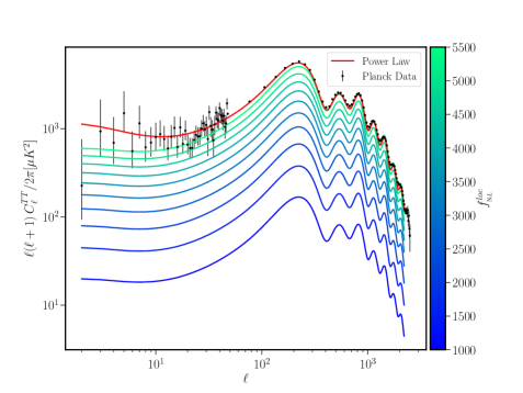
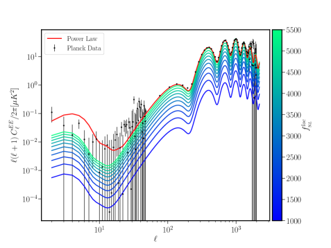
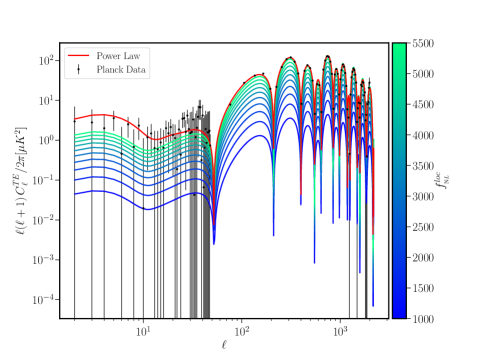
Utilizing the $\mathcal{P}_{{}_{\mathrm{S}}}(k)$ and $\mathcal{P}_{{}_{\mathrm{C}}}^{\rm loc}(k)$, we compute the respective CMB angular spectra using CAMB. Since we focus on the scalar power and the associated non-Gaussian correction we compute just the three related correlations of the CMB angular spectrum, namely $TT,TE$ and $EE$ correlations. For subsequent templates and models, we shall focus only on $TT$ correlations to examine the effects of corresponding $\mathcal{P}_{{}_{\mathrm{C}}}(k)$. In Fig. 1, we present the angular spectra obtained from $\mathcal{P}_{{}_{\mathrm{C}}}^{\rm loc}(k)$ along with those obtained from $\mathcal{P}_{{}_{\mathrm{S}}}(k)$. Note that these are separate contributions from the original and non-Gaussian parts of the power spectrum and the complete power spectrum shall be the sum of both. We find that the amplitude of $C_{\ell}$s increases as $f_{{}_{\rm NL}}^{\rm loc}$ is increased. But the value of $f_{{}_{\rm NL}}^{\rm loc}$ required to give rise to $C_{\ell}$s of magnitude comparable to the original spectrum is around $5000$. This value is evidently much higher than the bound obtained from direct constraint, i.e. $f_{{}_{\rm NL}}^{\rm loc}=-0.9\pm 5.1$. Therefore, we find that our method is not particularly useful in constraining this template.

III.2 Orthogonal type

We turn to the template of orthogonal type $f_{{}_{\rm NL}}(k_{1},k_{2},k_{3})$ which is known to arise in models with non-Bunch Davies initial states for perturbations [52, 53, 24]. The scalar bispectrum for this case is parametrized as [22]

$${\cal B}^{\rm ortho}\left(k_{1},k_{2},k_{3}\right) = \frac{6A_{s}^{2}f_{{}_{\rm NL}}^{\rm ortho}}{k_{*}^{2(n_{{}_{\mathrm{S}}}-1)}}\left\{-\frac{3}{\left(k_{1}k_{2}\right)^{4-n_{{}_{\mathrm{S}}}}}-\frac{3}{\left(k_{2}k_{3}\right)^{4-n_{{}_{\mathrm{S}}}}}-\frac{3}{\left(k_{3}k_{1}\right)^{4-n_{{}_{\mathrm{S}}}}}-\frac{8}{\left(k_{1}k_{2}k_{3}\right)^{\frac{2}{3}\left(4-n_{{}_{\mathrm{S}}}\right)}}\right.$$ (11)

$$\left.+\left[\frac{3}{k_{1}^{\left(4-n_{{}_{\mathrm{S}}}\right)/3}k_{2}^{2\left(4-n_{{}_{\mathrm{S}}}\right)/3}k_{3}^{4-n_{{}_{\mathrm{S}}}}}+5\text{ permutations }\right]\right\}.$$

The original scalar power is assumed to be the nearly scale invariant spectrum as in Eq. (9). So, the form of the non-Gaussianity parameter [cf. Eq. (4)], in terms of the variables of integration $x,y$ as it appears in Eq. (8), becomes

$$f_{{}_{\rm NL}}(k,kx,ky) = \frac{160\sqrt{2\pi}f_{{}_{\rm NL}}^{\rm ortho}x^{3}y^{3}}{1+x^{3}+y^{3}}\left\{\frac{1}{x^{2}y^{2}}+\frac{3}{8}\left(\frac{1}{x^{3}}+\frac{1}{y^{3}}+\frac{1}{x^{3}y^{3}}\right)-\frac{3}{8}\left(\frac{1}{x^{3}y}+\frac{1}{xy^{3}}+\frac{1}{x^{2}y}+\frac{1}{xy^{2}}+\frac{1}{x^{3}y^{2}}+\frac{1}{x^{2}y^{3}}\right)\right\}.\;\;\;\;\;\;$$ (12)

In the above expression, we have ignored the tilt in $x$ and $y$ in the above, i.e. we have set $x^{n_{{}_{\mathrm{S}}}-1}=y^{n_{{}_{\mathrm{S}}}-1}=1$. For our analysis to infer the dominant effect due to the crucial parameter $f_{{}_{\rm NL}}^{\rm ortho}$, these minor contributions do not change the results appreciably. Evidently, the parameter $f_{{}_{\rm NL}}^{\rm ortho}$ that determines the strength of the non-Gaussianity, shall determine the amplitude of $\mathcal{P}_{{}_{\mathrm{C}}}(k)$. With nearly scale invariant $\mathcal{P}_{{}_{\mathrm{S}}}(k)$ and $f_{{}_{\rm NL}}(k,kx,ky)$ above, we calculate the $\mathcal{P}_{{}_{\mathrm{C}}}(k)$ to be

$$\mathcal{P}_{{}_{\mathrm{C}}}^{\rm ortho}(k) = \frac{9}{25}(160)^{2}(2\pi)(f_{{}_{\rm NL}}^{\rm ortho})^{2}A_{s}^{2}\left(\frac{k}{k_{*}}\right)^{2(n_{{}_{\mathrm{S}}}-1)}\int_{0}^{\infty}dx\int_{|1-x|}^{(1+x)}dy\frac{1}{x^{2}y^{2}}\frac{x^{6}y^{6}}{(1+x^{3}+y^{3})^{2}}$$ (13)

$$\times\left[\frac{1}{x^{2}y^{2}}+\frac{3}{8}\left(\frac{1}{x^{3}}+\frac{1}{y^{3}}+\frac{1}{x^{3}y^{3}}\right)-\frac{3}{8}\left(\frac{1}{x^{3}y}+\frac{1}{xy^{3}}+\frac{1}{x^{2}y}+\frac{1}{xy^{2}}+\frac{1}{x^{3}y^{2}}+\frac{1}{x^{2}y^{3}}\right)\right]^{2}.$$

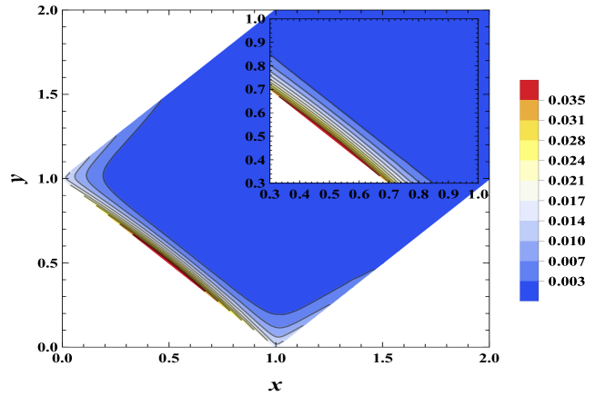
We find that the integral does not diverge anywhere in the range of integration, unlike local type (see App. A for the shape of the integrand). Instead it has a maximum value of ${1}/{25}$ at $x=y=1/2$. The rise is sharp along $y=1-x$, so we can approximate the integral involved in $\mathcal{P}_{{}_{\mathrm{C}}}(k)$ as

$$\mathcal{P}_{{}_{\mathrm{C}}}^{\rm ortho}(k) = \frac{9}{25}(160)^{2}(2\pi)(f_{{}_{\rm NL}}^{\rm ortho})^{2}\mathcal{P}_{{}_{\mathrm{S}}}^{2}(k)\int_{0}^{\infty}dx\int_{|1-x|}^{(1+x)}dy\delta(y-(1-x))\frac{1}{x^{2}y^{2}}\frac{x^{6}y^{6}}{(1+x^{3}+y^{3})^{2}}$$ (15)

$$\times\left[\frac{1}{x^{2}y^{2}}+\frac{3}{8}\left(\frac{1}{x^{3}}+\frac{1}{y^{3}}+\frac{1}{x^{3}y^{3}}\right)-\frac{3}{8}\left(\frac{1}{x^{3}y}+\frac{1}{xy^{3}}+\frac{1}{x^{2}y}+\frac{1}{xy^{2}}+\frac{1}{x^{3}y^{2}}+\frac{1}{x^{2}y^{3}}\right)\right]^{2}$$

$$= \frac{9}{25}(160)^{2}(2\pi)(f_{{}_{\rm NL}}^{\rm ortho})^{2}\mathcal{P}_{{}_{\mathrm{S}}}^{2}(k)\int_{0}^{\infty}dx\frac{1}{x^{2}(1-x)^{2}}\frac{x^{6}(1-x)^{6}}{(1+x^{3}+(1-x)^{3})^{2}}$$

$$\times\left[\frac{1}{x^{2}(1-x)^{2}}+\frac{3}{8}\left(\frac{1}{x^{3}}+\frac{1}{(1-x)^{3}}+\frac{1}{x^{3}(1-x)^{3}}\right)\right.$$

$$-\left.\frac{3}{8}\left(\frac{1}{x^{3}(1-x)}+\frac{1}{x(1-x)^{3}}+\frac{1}{x^{2}(1-x)}+\frac{1}{x(1-x)^{2}}+\frac{1}{x^{3}(1-x)^{2}}+\frac{1}{x^{2}(1-x)^{3}}\right)\right]^{2}$$

$$= \frac{9}{25}(160)^{2}(2\pi)(f_{{}_{\rm NL}}^{\rm ortho})^{2}\mathcal{P}_{{}_{\mathrm{S}}}^{2}(k)\int_{0}^{\infty}dx\frac{1}{16(3x^{2}-3x+2)^{2}}$$ (16)

$$= 1.84\times 10^{4}\pi\,(f_{{}_{\rm NL}}^{\rm ortho})^{2}\mathcal{P}_{{}_{\mathrm{S}}}^{2}(k)\,{\cal I}^{\rm ortho}\,,$$ (17)

where ${\cal I}^{\rm ortho}\simeq 2.95\times 10^{-2}$ . Hence,

$$\mathcal{P}_{{}_{\mathrm{C}}}^{\rm ortho}(k) \simeq 1.71\times 10^{3}\,\mathcal{P}_{{}_{\mathrm{S}}}^{2}(k)\,(f_{{}_{\rm NL}}^{\rm ortho})^{2}.$$ (18)

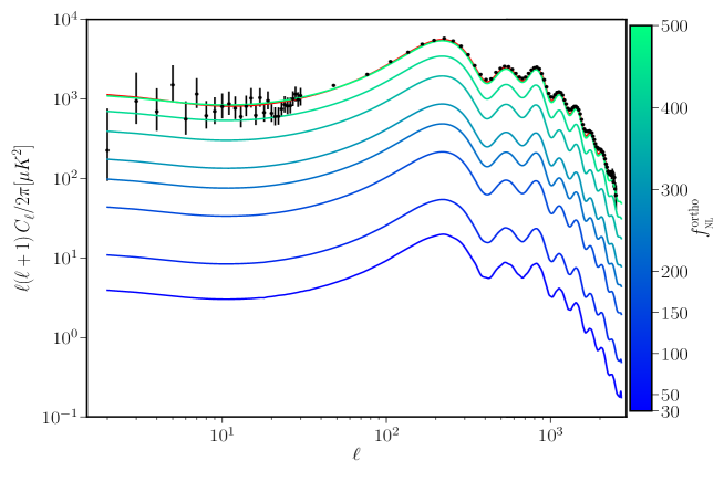
Figure 2: The $TT$ angular power spectrum arising from $\mathcal{P}_{{}_{\mathrm{C}}}^{\rm ortho}$ is presented (in shades of blue to green) across a range of the parameter $f_{{}_{\rm NL}}^{\rm ortho}$. The standard spectrum due to $\mathcal{P}_{{}_{\mathrm{S}}}(k)$ is presented (in red) along with the Planck data points (in black). As expected, the amplitude of $C_{\ell}$s due to $\mathcal{P}_{{}_{\mathrm{C}}}^{\rm ortho}(k)$ decreases as $f_{{}_{\rm NL}}^{\rm ortho}$ is decreased. An interesting point to note is that the value of $f_{{}_{\rm NL}}^{\rm ortho}$ required to get amplitudes comparable to the standard $C_{\ell}$s is $\sim 500$, which is an order of magnitude lesser than it is required for $f_{{}_{\rm NL}}^{\rm loc}$.

The CMB angular spectrum due to $\mathcal{P}_{{}_{\mathrm{C}}}^{\rm ortho}(k)$ is presented in Fig. 2. We find that the amplitude of $f_{{}_{\rm NL}}^{\rm ortho}$ required to generate $C_{\ell}$s of amplitude comparable to the original spectrum is around $500$. This is an order of magnitude lesser than that of the local type. It is mainly due to the structure and numerical coefficients in the definition of the scalar bispectrum of this template. Yet, this value of $f_{{}_{\rm NL}}^{\rm ortho}$ is larger than the present constraint of $f_{{}_{\rm NL}}^{\rm ortho}=-39\pm 64$ at $1$-$\sigma$ level.

III.3 Equilateral type

We next consider $f_{{}_{\rm NL}}(k_{1},k_{2},k_{3})$ of equilateral template which is representative of non-Gaussianity arising from canonical single field inflationary models with typical slow-roll evolution at early times [20, 13, 5, 23]. The scalar bispectrum for this case is parametrized as [22]

$${\cal B}^{\rm eq}(k_{1},k_{2},k_{3}) = 6\,A_{s}^{2}\,f_{{}_{\rm NL}}^{\rm eq}\,\bigg{\{}-\frac{1}{(k_{1}k_{2})^{3}}\,\left(\frac{k_{1}k_{2}}{k^{2}_{\ast}}\right)^{n_{{}_{\mathrm{S}}}-1}-\frac{1}{(k_{2}k_{3})^{3}}\,\left(\frac{k_{2}k_{3}}{k^{2}_{\ast}}\right)^{n_{{}_{\mathrm{S}}}-1}-\frac{1}{(k_{1}k_{3})^{3}}\,\left(\frac{k_{1}k_{3}}{k^{2}_{\ast}}\right)^{n_{{}_{\mathrm{S}}}-1}$$ (19)

$$-\frac{2}{(k_{1}\,k_{2}\,k_{3})^{2}}\,\left(\frac{k_{1}k_{2}k_{3}}{k^{3}_{\ast}}\right)^{2(n_{{}_{\mathrm{S}}}-1)/3}+\bigg{[}\frac{1}{k_{1}k_{2}^{2}k_{3}^{3}}\left(\frac{k_{1}\,k_{2}^{2}k_{3}^{3}}{k_{\ast}^{6}}\right)^{(n_{{}_{\mathrm{S}}}-1)/3}+\leavevmode\nobreak\ (5\leavevmode\nobreak\ {\rm permutations})\bigg{]}\bigg{\}}.$$

This template of bispectrum, along with the nearly scale invariant spectrum of Eq. (9), when substituted in the expression of $f_{{}_{\rm NL}}$ in terms of $k,kx,ky$ as required in the integral of interest, gives us [cf. Eq. (4)]

$$f_{{}_{\rm NL}}(k,kx,ky) = \frac{20\sqrt{2\pi}f_{{}_{\rm NL}}^{\rm eq}x^{3}y^{3}}{(1+x^{3}+y^{3})}\bigg{\{}\frac{1}{x^{3}}+\frac{1}{y^{3}}+\frac{1}{x^{3}y^{3}}+\frac{2}{x^{2}y^{2}}-\left[\frac{1}{x^{2}y^{3}}+\leavevmode\nobreak\ (5\leavevmode\nobreak\ {\rm permutations})\right]\bigg{\}}\,.$$ (20)

This $f_{{}_{\rm NL}}(k,kx,ky)$ leads to $\mathcal{P}_{{}_{\mathrm{C}}}(k)$ of the form

$$\mathcal{P}_{{}_{\mathrm{C}}}^{\rm eq}(k)=288\pi\,\mathcal{P}_{{}_{\mathrm{S}}}^{2}(k)\,(f_{{}_{\rm NL}}^{\rm eq})^{2}\,\int_{0}^{\infty}{\rm d}x\int_{|1-x|}^{1+x}{\rm d}y \left(\frac{1}{x^{2}y^{2}}\right)\,\frac{x^{6}y^{6}}{(1+x^{3}+y^{3})^{2}}\bigg{\{}\frac{1}{x^{3}}+\frac{1}{y^{3}}+\frac{1}{x^{3}y^{3}}+\frac{2}{x^{2}y^{2}}$$ (21)

$$-\left[\frac{1}{xy^{3}}+\frac{1}{x^{3}y}+\frac{1}{xy^{2}}+\frac{1}{x^{2}y}+\frac{1}{x^{2}y^{3}}+\frac{1}{x^{3}y^{2}}\right]\bigg{\}}^{2}\,,$$

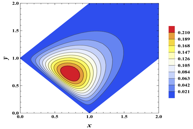
where, as in the previous case, we have ignored the minor tilt arising due to $x^{n_{{}_{\mathrm{S}}}-1}$ and $y^{n_{{}_{\mathrm{S}}}-1}$ without losing much information about the amplitude or scale dependence of $\mathcal{P}_{{}_{\mathrm{C}}}^{\rm eq}(k)$. The above integrand does not diverge in the regime of integration and has a maximum of about $0.236$ at $(x,y)\simeq(0.719,0.719)$. Away from this maximum, the function quickly decays down (see App. A for related details). So, we approximate the integral as this maximum value and integrate over a unit area around this point to obtain a simplified expression of $\mathcal{P}_{{}_{\mathrm{C}}}^{\rm eq}(k)$ as

$$\mathcal{P}_{{}_{\mathrm{C}}}^{\rm eq}(k) \simeq 2.135\times 10^{2}\,\mathcal{P}_{{}_{\mathrm{S}}}^{2}(k)(f_{{}_{\rm NL}}^{\rm eq})^{2}\,.$$ (22)

Figure 3: The angular spectrum due to $\mathcal{P}_{{}_{\mathrm{C}}}^{\rm eq}(k)$ is presented (in shades of blue to green) across a range of the parameter $f_{{}_{\rm NL}}^{\rm eq}$ along with the standard spectrum due to $\mathcal{P}_{{}_{\mathrm{S}}}(k)$ (in red) and the data points (in black). At $f_{{}_{\rm NL}}^{\rm eq}\sim 1400$, the $C_{\ell}$ due to $\mathcal{P}_{{}_{\mathrm{C}}}^{\rm eq}(k)$ become comparable to the amplitude of the standard $C_{\ell}$s. This is similar to the value that is required for $f_{{}_{\rm NL}}^{\rm loc}$.

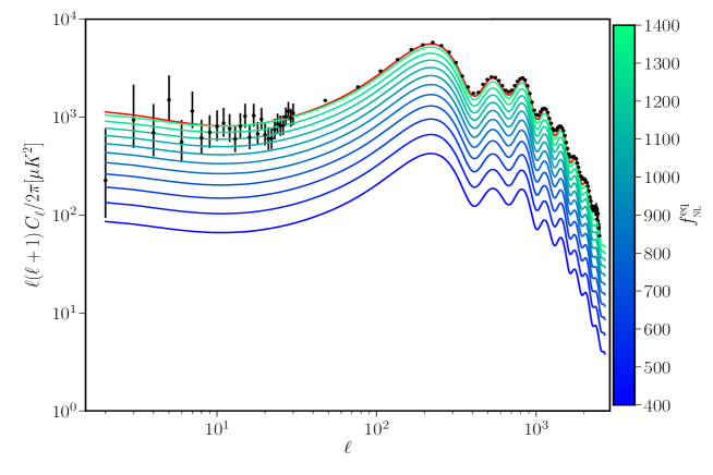
The CMB angular spectrum in this case is presented in Fig. 3. We find that the amplitude of $f_{{}_{\rm NL}}^{\rm eq}$ required to produce $C_{\ell}$s of magnitude comparable to the standard $C_{\ell}$s due to $\mathcal{P}_{{}_{\mathrm{S}}}(k)$ is around $10^{3}$. Once again this value is higher than the direct constraint on the parameter, $f_{{}_{\rm NL}}^{\rm eq}=-26\pm 47$ at $1$-$\sigma$ level. However, it is about a factor of $5$ lesser than the value of $f_{{}_{\rm NL}}^{\rm loc}$ required to lead to similar effect in $C_{\ell}$s. Thus we see that the templates with weaker bounds through direct constraints may be constrained better through our indirect method.

III.4 Templates with running

Apart from the explicit scale dependence of the templates discussed above, a mild running of $f_{{}_{\rm NL}}(k_{1},k_{2},k_{3})$ is typically be introduced as [54, 22]

$$f_{{}_{\rm NL}}^{\rm type-run}(k_{1},k_{2},k_{3}) = f_{{}_{\rm NL}}^{\rm type}(k_{1},k_{2},k_{3})\left(\frac{k_{1}+k_{2}+k_{3}}{3\,k_{\ast}}\right)^{n_{\rm NG}}\,,$$ (23)

where $n_{\rm NG}$ quantifies the running of the parameter about $k_{\ast}$ and ‘type’ can refer to one of local, equilateral or orthogonal templates. The typical value of $n_{\rm NG}$ is between $-0.1$ and $0.1$ and the constraints on them are broad and consistent with zero [22]. In our method, it can be easily derived that introduction of such a running to the templates modifies the corresponding $\mathcal{P}_{{}_{\mathrm{C}}}(k)$ as

$$\mathcal{P}_{{}_{\mathrm{C}}}^{\rm type-run}(k) = \mathcal{P}_{{}_{\mathrm{C}}}^{\rm type}(k)\left(\frac{k}{3\,k_{\ast}}\right)^{2n_{\rm NG}}\,.$$ (24)

Once again we have ignored the minor dependence of $n_{\rm NG}$ through the variables of integration, i.e. $x^{n_{\rm NG}},y^{n_{\rm NG}}$ in performing the integral and focus on capturing the prominent scale dependence through $k^{n_{\rm NG}}$.

Figure 4: The angular spectrum due to $\mathcal{P}_{{}_{\mathrm{C}}}(k)$ is presented (in shades of blue to green) for the case of running of $f_{{}_{\rm NL}}$ across a range of parameter $n_{\rm NG}$. We present it for the case of local (on top left), orthogonal (on top right) and equilateral (at the bottom) templates along with the standard $C_{\ell}$s due to power law $\mathcal{P}_{{}_{\mathrm{S}}}(k)$ (in red) and data points (in black). We have fixed the respective $f_{{}_{\rm NL}}$ amplitudes to be $f_{{}_{\rm NL}}^{\rm loc}=5000$, $f_{{}_{\rm NL}}^{\rm ortho}=400$ and $f_{{}_{\rm NL}}^{\rm eq}=1000$ to illustrate the effect of $n_{\rm NG}$ on the $C_{\ell}$s.

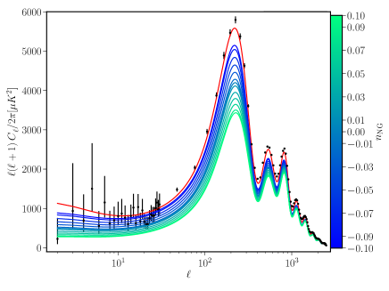
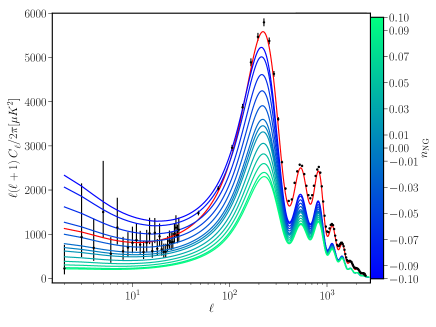
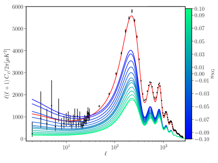
The $C_{\ell}$s due to $\mathcal{P}_{{}_{\mathrm{C}}}^{\rm type-run}(k)$ have been presented in Fig. 4, for local, orthogonal and equilateral templates. We fix the values of $f_{{}_{\rm NL}}^{\rm type}$ in respective templates and focus on the effect due to variation of ${n_{\rm NG}}$. We find that for a given template, ${n_{\rm NG}}$ can alter the overall tilt of the angular spectrum and this in turn affects the amplitude of $C_{\ell}$s over large scales. Therefore, while comparing against data, the running may have significant impact and may be degenerate to some extent with $f_{{}_{\rm NL}}^{\rm type}$ in its constraints.

For the templates studied so far, we find that the value of the respective amplitudes of non-Gaussianity $f_{{}_{\rm NL}}^{\rm type}$, that is required to produce discernible effect on the $C_{\ell}$s to be much higher than the existing bounds on them arrived at from direct comparison against data by Planck [22]. However, this exercise gives us insights on the computation of the integrals involved and helps us to employ the technique to $f_{{}_{\rm NL}}(k_{1},k_{2},k_{3})$ with non-trivial scale dependences as we shall discuss next.

III.5 Oscillatory Type

We turn to a rather interesting case of oscillatory features in the power spectrum and the bispectrum. Such spectra are observed in models of inflation containing oscillatory features in potentials, sharp transitions during the field evolution or non-inflationary initial epoch [55, 53, 56, 5]. The scalar power in this case is parametrized as

$$\mathcal{P}_{{}_{\mathrm{S}}}^{\rm osc}(k)=A_{{}_{\rm S}}\left(\frac{k}{k_{\ast}}\right)^{n_{{}_{\mathrm{S}}}-1}\,\left\{1+b\,\sin\left[\omega\ln\left(\frac{k}{k_{o}}\right)\right]\right\}\,,$$ (25)

where $b$ quantifies the strength and $\omega$ the frequency of the oscillatory feature. The scalar bispectrum is modelled as [22]

$${\cal B}^{\rm osc}(k_{1},k_{2},k_{3})=\frac{6A_{{}_{\rm S}}^{2}f_{{}_{\rm NL}}^{\rm osc}}{(k_{1}k_{2}k_{3})^{2}}\sin\left[\omega\ln\left(\frac{k_{1}+k_{2}+k_{3}}{k_{o}}\right)\right]\,.$$ (26)

Evidently the amplitude of the bispectrum and hence the associated $f_{{}_{\rm NL}}(k_{1},k_{2},k_{3})$ is determined by $f_{{}_{\rm NL}}^{\rm osc}$. We should note that in the above expression the factor $A_{{}_{\rm S}}$ is included while ignoring the tilt and running of the bispectrum. So, when we compute $f_{{}_{\rm NL}}(k_{1},k_{2},k_{3})$, the tilt in the power spectra in the denominator shall also be consistently ignored. In other words, if we include the tilt of $(k/k_{\ast})^{(n_{{}_{\mathrm{S}}}-1)}$ in the parametrization of the bispectrum, then it will be cancelled by corresponding term arising from the power spectra in the denominator [cf. Eq. (4)]. Thus, the $f_{{}_{\rm NL}}(k_{1},k_{2},k_{3})$ in this case shall be

$$f_{{}_{\rm NL}}(k_{1},k_{2},k_{3}) = -20\sqrt{2\pi}(k_{1}k_{2}k_{3})A_{{}_{\rm S}}^{2}f_{{}_{\rm NL}}^{\rm osc}\frac{\sin\left[\omega\ln\left(\frac{k_{1}+k_{2}+k_{3}}{k_{o}}\right)\right]}{\left[k_{1}^{3}\mathcal{P}_{{}_{\mathrm{S}}}^{\rm osc}(k_{2})\mathcal{P}_{{}_{\mathrm{S}}}^{\rm osc}(k_{3})+k_{2}^{3}\mathcal{P}_{{}_{\mathrm{S}}}^{\rm osc}(k_{1})\mathcal{P}_{{}_{\mathrm{S}}}^{\rm osc}(k_{3})+k_{3}^{3}\mathcal{P}_{{}_{\mathrm{S}}}^{\rm osc}(k_{1})\mathcal{P}_{{}_{\mathrm{S}}}^{\rm osc}(k_{2})\right]}$$ (27)

$$= -20\sqrt{2\pi}(k_{1}k_{2}k_{3})f_{{}_{\rm NL}}^{\rm osc}\frac{\sin\left[\omega\ln\left(\frac{k_{1}+k_{2}+k_{3}}{k_{o}}\right)\right]}{\left\{k_{1}^{3}\,\left[1+b\sin\left(\omega\ln\frac{k_{2}}{k_{o}}\right)\right]\left[1+b\sin\left(\omega\ln\frac{k_{3}}{k_{o}}\right)\right]+2\leavevmode\nobreak\ {\rm permutations}\right\}}\,.$$ (28)

Substituting $\mathcal{P}_{{}_{\mathrm{S}}}^{\rm osc}(k)$ and $f_{{}_{\rm NL}}(k_{1},k_{2},k_{3})$ above in Eq. (8), we obtain $\mathcal{P}_{{}_{\mathrm{C}}}^{\rm osc}(k)$ of the form

$$\mathcal{P}_{{}_{\mathrm{C}}}^{\rm osc}(k) = 288\,\pi\,\,\bigg{[}A_{{}_{\rm S}}\left(\frac{k}{k_{\ast}}\right)^{n_{{}_{\mathrm{S}}}-1}f_{{}_{\rm NL}}^{\rm osc}\bigg{]}^{2}\int_{0}^{\infty}{\rm d}x\int^{1+x}_{|1-x|}{\rm d}y\,xy\left[1+b\sin\left(\omega\ln\frac{kx}{k_{o}}\right)\right]\left[1+b\sin\left(\omega\ln\frac{ky}{k_{o}}\right)\right]$$ (29)

$$\times\sin^{2}\left[\omega\ln\left(\frac{k}{k_{o}}(1+x+y)\right)\right]\Bigg{\{}\left[1+b\sin\left(\omega\ln\frac{kx}{k_{o}}\right)\right]\left[1+b\sin\left(\omega\ln\frac{ky}{k_{o}}\right)\right]$$

$$+x^{3}\,\left[1+b\sin\left(\omega\ln\frac{k}{k_{o}}\right)\right]\left[1+b\sin\left(\omega\ln\frac{ky}{k_{o}}\right)\right]+y^{3}\,\left[1+b\sin\left(\omega\ln\frac{k}{k_{o}}\right)\right]\left[1+b\sin\left(\omega\ln\frac{kx}{k_{o}}\right)\right]\Bigg{\}}^{-1}.\;\;\;\;\;\;$$

Note that we have ignored the terms such as $x^{n_{{}_{\mathrm{S}}}-1}$ and $y^{n_{{}_{\mathrm{S}}}-1}$ as in the cases before, since we are interested in the order of magnitude of the above integral and these terms provide negligible contribution to this estimate. Moreover, the integrand does not diverge at $(x,y)=(0,1)$ or $(1,0)$ due to the well behaved shape of the bispectrum (cf. App. A).

To perform the double integral above, we shall utilize the fact that the parameter $b$ typically takes values $b<1$. So, we shall first focus on the terms of order $b^{0}$ and then proceed to higher order terms in our calculation of $\mathcal{P}_{{}_{\mathrm{C}}}^{\rm osc}(k)$. The $f_{{}_{\rm NL}}(k,kx,ky)$ as it appears in the integral of $\mathcal{P}_{{}_{\mathrm{C}}}^{\rm osc}(k)$, can then be expanded as

$$f_{{}_{\rm NL}}(k,kx,ky) = -20\sqrt{2\pi}\,f_{{}_{\rm NL}}^{\rm osc}\frac{xy}{1+x^{3}+y^{3}}\bigg{[}\sin\left(\omega\ln\frac{k}{k_{o}}\right)\cos\left[\omega\ln(1+x+y)\right]$$ (30)

$$+\cos\left(\omega\ln\frac{k}{k_{o}}\right)\sin\left[\omega\ln(1+x+y)\right]\bigg{]}+{\cal O}(b)+{\cal O}(b^{2})\,.$$

We obtain the correction to the scalar power $\mathcal{P}_{{}_{\mathrm{C}}}(k)$ at the leading order of ${\cal O}(b^{0})$ to be

$$\mathcal{P}_{{}_{\mathrm{C}}}^{\rm osc}(k) \simeq 2\pi\left[12\,A_{{}_{\rm S}}\left(\frac{k}{k_{\ast}}\right)^{(n_{{}_{\mathrm{S}}}-1)}f_{{}_{\rm NL}}^{\rm osc}\right]^{2}\int_{0}^{\infty}{\rm d}x\int^{1+x}_{|1-x|}{\rm d}y\frac{1}{(1+x^{3}+y^{3})^{2}}$$ (31)

$$\times\bigg{[}\sin\left(\omega\ln\frac{k}{k_{o}}\right)\cos\left[\omega\ln(1+x+y)\right]+\cos\left(\omega\ln\frac{k}{k_{o}}\right)\sin\left[\omega\ln(1+x+y)\right]\bigg{]}^{2}\,.$$

On simplifying the integral further, we obtain

$$\mathcal{P}_{{}_{\mathrm{C}}}^{\rm osc}(k) = \pi\left[12\,A_{{}_{\rm S}}\left(\frac{k}{k_{\ast}}\right)^{(n_{{}_{\mathrm{S}}}-1)}f_{{}_{\rm NL}}^{\rm osc}\right]^{2}\bigg{[}{\cal I}_{1}-\cos\left(2\omega\ln\frac{k}{k_{o}}\right){\cal I}_{2}+\sin\left(2\omega\ln\frac{k}{k_{o}}\right){\cal I}_{3}\bigg{]}\,,$$ (32)

where the terms $\cal I$s are integrals whose explicit forms are provided in App. A. We know that the integrands of $\cal I$ are unity at maximum and hence the terms themselves evaluate to ${\cal O}(1)$ values. As can be expected, $\mathcal{P}_{{}_{\mathrm{C}}}^{\rm osc}(k)$, at the leading order, has an oscillatory pattern of frequency $2\omega$, while the original spectrum $\mathcal{P}_{{}_{\mathrm{S}}}^{\rm osc}(k)$ has a frequency of $\omega$.

Now let us turn to the terms of ${\cal O}(b)$. The parameter $f_{{}_{\rm NL}}(k,kx,ky)$ expanded up to linear order in $b$ is

$$f_{{}_{\rm NL}}(k,kx,ky) = -20\sqrt{2\pi}f_{{}_{\rm NL}}^{\rm osc}\frac{xy}{(1+x^{3}+y^{3})}\sin\left[\omega\ln\left(\frac{k}{k_{o}}\right)+\omega\ln(1+x+y)\right]$$ (33)

$$\times\Bigg{\{}1-\frac{b}{(1+x^{3}+y^{3})}\Bigg{[}\sin\left[\omega\ln\left(\frac{k}{k_{o}}\right)+\omega\ln x\right]+\sin\left[\omega\ln\left(\frac{k}{k_{o}}\right)+\omega\ln y\right]$$

$$+(x^{3}+y^{3})\sin\left[\omega\ln\left(\frac{k}{k_{o}}\right)\right]+x^{3}\sin\left[\omega\ln\left(\frac{k}{k_{o}}\right)+\omega\ln y\right]+y^{3}\sin\left[\omega\ln\left(\frac{k}{k_{o}}\right)+\omega\ln x\right]\Bigg{]}\Bigg{\}}.$$

Substituting this expression in $\mathcal{P}_{{}_{\mathrm{C}}}(k)$ along with $\mathcal{P}_{{}_{\mathrm{S}}}^{\rm osc}(k)$ terms expanded to the same order in $b$, we obtain

$$\mathcal{P}_{{}_{\mathrm{C}}}^{\rm osc}(k) = 288\,\pi\,\,\bigg{[}A_{{}_{\rm S}}\left(\frac{k}{k_{\ast}}\right)^{n_{{}_{\mathrm{S}}}-1}f_{{}_{\rm NL}}^{\rm osc}\bigg{]}^{2}\int_{0}^{\infty}{\rm d}x\int^{1+x}_{|1-x|}{\rm d}y\frac{1}{x^{2}y^{2}}\Bigg{[}\frac{xy}{1+x^{3}+y^{3}}\sin\bigg{[}\omega\ln\left(\frac{k}{k_{o}}\right)+\omega\ln(1+x+y)\bigg{]}\Bigg{]}^{2}$$ (34)

$$\times\Bigg{\{}1-\frac{b}{(1+x^{3}+y^{3})}\Bigg{[}\sin\left[\omega\ln\left(\frac{k}{k_{o}}\right)+\omega\ln x\right]+\sin\left[\omega\ln\left(\frac{k}{k_{o}}\right)+\omega\ln y\right]$$

$$+(x^{3}+y^{3})\sin\left[\omega\ln\left(\frac{k}{k_{o}}\right)\right]+x^{3}\sin\left[\omega\ln\left(\frac{k}{k_{o}}\right)+\omega\ln y\right]+y^{3}\sin\left[\omega\ln\left(\frac{k}{k_{o}}\right)+\omega\ln x\right]\Bigg{]}\Bigg{\}}^{2}.$$

In this integral, we retain only terms up to ${\cal O}(b)$ and ignore terms with ${\cal O}(b^{2})$ or higher order. We also ignore ${\cal O}(b^{0})$ as they have been already taken care of. Grouping these terms and simplifying, we obtain $\mathcal{P}_{{}_{\mathrm{C}}}^{\rm osc}(k)$ at the order of ${\cal O}(b)$ to be

$$\mathcal{P}_{{}_{\mathrm{C}}}^{\rm osc}(k) \simeq -\pi\,b\,\left[24\,A_{{}_{\rm S}}\left(\frac{k}{k_{\ast}}\right)^{(n_{{}_{\mathrm{S}}}-1)}f_{{}_{\rm NL}}^{\rm osc}\right]^{2}\bigg{[}\sin^{3}\left(\omega\ln\frac{k}{k_{o}}\right){\cal I}^{(b)}_{1}+\sin^{2}\left(\omega\ln\frac{k}{k_{o}}\right)\cos\left(\omega\ln\frac{k}{k_{o}}\right){\cal I}^{(b)}_{2}$$ (35)

$$+\sin\left(\omega\ln\frac{k}{k_{o}}\right)\cos^{2}\left(\omega\ln\frac{k}{k_{o}}\right){\cal I}^{(b)}_{3}+\cos^{3}\left(\omega\ln\frac{k}{k_{o}}\right){\cal I}^{(b)}_{4}+\sin^{2}\left(\omega\ln\frac{k}{k_{o}}\right)\cos\left(\omega\ln\frac{k}{k_{o}}\right){\cal I}^{(b)}_{5}$$

$$+\sin\left(\omega\ln\frac{k}{k_{o}}\right)\cos^{2}\left(\omega\ln\frac{k}{k_{o}}\right){\cal I}^{(b)}_{6}\bigg{]}\,.$$

Here the integrals ${\cal I}^{(b)}$s are again ${\cal O}(1)$ quantities whose exact expressions are given in App. A. We find that the corrections of ${\cal O}(b)$ are of frequency $3\omega$. The total $\mathcal{P}_{{}_{\mathrm{C}}}^{\rm osc}(k)$ shall be the sum of the terms obtained in Eqs. (32) and (35). We restrict our calculation up to ${\cal O}(b)$ and compute the angular spectrum arising due to this $\mathcal{P}_{{}_{\mathrm{C}}}^{\rm osc}(k)$. Since, the quantities $\cal I$s are ${\cal O}(1)$ we set their values to unity in our computation of $C_{\ell}$s. This approximation is done just to understand the general behavior and parametric dependences of $C_{\ell}$s in this case. One should perform these integrals exactly while comparing against the data to arrive at constraints on the parameters.

Figure 5: The $\mathcal{P}_{{}_{\mathrm{S}}}^{\rm osc}(k)$ (in shades of red to yellow) and $\mathcal{P}_{{}_{\mathrm{C}}}^{\rm osc}(k)$ (in shades of blue to green) are presented for different values of $b$ (on left) and $\omega$ (on right). Note that in the expression of $\mathcal{P}_{{}_{\mathrm{C}}}^{\rm osc}(k)$, $b$ determines the strength of oscillations of the component that has frequency of $3\omega$. Hence, increase in $b$ enhances this part of $\mathcal{P}_{{}_{\mathrm{C}}}^{\rm osc}(k)$ while the contribution with frequency of $2\omega$ remains unaffected in amplitude. We set $\omega=5$ to arrive at this behavior. On the other hand, as $\omega$ is increased, the oscillatory patterns are more pronounced in $\mathcal{P}_{{}_{\mathrm{C}}}(k)$ than in $\mathcal{P}_{{}_{\mathrm{S}}}(k)$. We set $b=0.05$ to obtain this plot. The other related parameters are set to be $f_{{}_{\rm NL}}^{\rm osc}=500$, and $k_{o}/\,{\rm Mpc}^{-1}=10^{-1}$ in obtaining these plots, so that the features of interest are better illustrated.

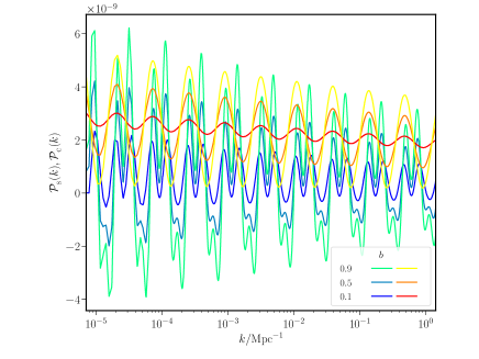
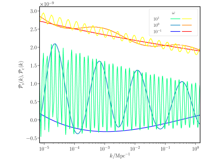
In Fig. 5 we show the variation of $\mathcal{P}_{{}_{\mathrm{S}}}^{\rm osc}(k)$ and $\mathcal{P}_{{}_{\mathrm{C}}}^{\rm osc}(k)$ for a range of parameters $b$ and $\omega$. The parameter $b$, in the expression of $\mathcal{P}_{{}_{\mathrm{C}}}^{\rm osc}(k)$, determines the strength of oscillations of the component that has frequency of $3\omega$. Hence, for a given value of $\omega$ increasing $b$ enhances this part of $\mathcal{P}_{{}_{\mathrm{C}}}^{\rm osc}(k)$ while the dominant contribution with frequency of $2\omega$ remains unaffected in amplitude. On the other hand, if we fix the value of $b$ and increase $\omega$, we observe that the oscillatory patterns are more pronounced in $\mathcal{P}_{{}_{\mathrm{C}}}^{\rm osc}(k)$ than in $\mathcal{P}_{{}_{\mathrm{S}}}^{\rm osc}(k)$. For both the plots, we have set $f_{{}_{\rm NL}}^{\rm osc}=500$, and $k_{o}/\,{\rm Mpc}^{-1}=10^{-1}$.

Figure 6: The angular spectrum due to $\mathcal{P}_{{}_{\mathrm{C}}}^{\rm osc}(k)$ is presented (in shades of blue to green) across a range of the parameter $f_{{}_{\rm NL}}^{\rm osc}$ along with the spectrum due to $\mathcal{P}_{{}_{\mathrm{S}}}^{\rm osc}(k)$ (in red) and the data points (in black). As expected, the amplitude of $C_{\ell}$s due to $\mathcal{P}_{{}_{\mathrm{C}}}^{\rm osc}(k)$ increases as this parameter is increased. However, the crucial point to note is that the range of $f_{{}_{\rm NL}}^{\rm osc}$ required to get amplitudes comparable to the standard $C_{\ell}$s is just $\sim 500$, which is realizable in models in the literature that produce such oscillatory bispectra. We have fixed other related parameters to be $b=5\times 10^{-2},\omega=5$ and $k_{o}/\,{\rm Mpc}^{-1}=10^{-1}$ in obtaining these plots.

Figure 7: The angular spectra due to $\mathcal{P}_{{}_{\mathrm{C}}}^{\rm osc}(k)$ and $\mathcal{P}_{{}_{\mathrm{S}}}^{\rm osc}(k)$ are presented (in shades of blue to green, and red to yellow respectively), across a range of the parameter $b$ which determines the strength of oscillations in $\mathcal{P}_{{}_{\mathrm{S}}}^{\rm osc}(k)$. Note that in the expression of $\mathcal{P}_{{}_{\mathrm{C}}}^{\rm osc}(k)$, $b$ determines the strength of oscillations of the component that has frequency of $3\omega$. Hence, variation of $b$ affects this part of $\mathcal{P}_{{}_{\mathrm{C}}}^{\rm osc}(k)$ while the contribution with frequency of $2\omega$ still remains unaffected in amplitude. The other related parameters are set to be $f_{{}_{\rm NL}}^{\rm osc}=500,\omega=5$ and $k_{o}/\,{\rm Mpc}^{-1}=10^{-1}$ in this figure.

Figure 8: The angular spectra due to $\mathcal{P}_{{}_{\mathrm{C}}}^{\rm osc}(k)$ and $\mathcal{P}_{{}_{\mathrm{S}}}^{\rm osc}(k)$ are presented (in shades of blue to green, and red to yellow respectively) across a range of the parameter $\omega$ which determines the frequency of oscillations in the power and the bi-spectra in this template. As the frequency is increased, the oscillatory patterns are more pronounced in $\mathcal{P}_{{}_{\mathrm{C}}}(k)$ than in $\mathcal{P}_{{}_{\mathrm{S}}}(k)$. We have set $f_{{}_{\rm NL}}^{\rm osc}=500,b=5\times 10^{-2}$ and $k_{o}/\,{\rm Mpc}^{-1}=10^{-1}$ in obtaining these plots.

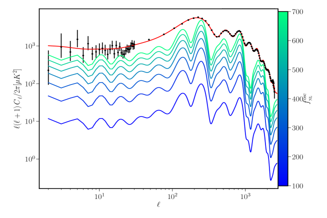
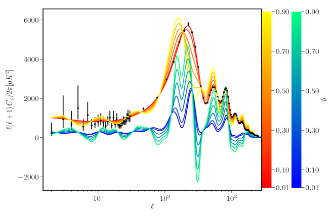
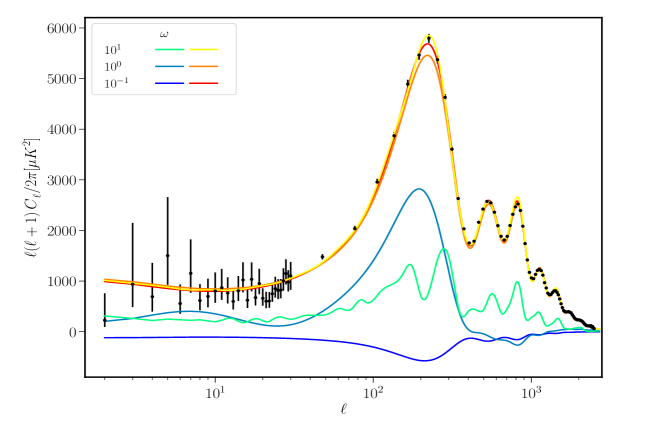
We illustrate the CMB angular spectra arising in this case in Figs. 6, 7 and 8. Note that along with the $C_{\ell}$s due to $\mathcal{P}_{{}_{\mathrm{C}}}^{\rm osc}(k)$, we plot the original $C_{\ell}$s in this case using $\mathcal{P}_{{}_{\mathrm{S}}}^{\rm osc}(k)$ as given in (25). We set the default values of the parameters to be $b=5\times 10^{-2},\,f_{{}_{\rm NL}}^{\rm osc}=500,\,\omega=5,k_{o}/\,{\rm Mpc}^{-1}=0.1$ about which we vary them individually to illustrate our results. As we have observed in previous cases, the amplitude of $C_{\ell}$s due to $\mathcal{P}_{{}_{\mathrm{C}}}^{\rm osc}(k)$ is directly proportional to the strength of the non-Gaussianity parameter, which in this case is $f_{{}_{\rm NL}}^{\rm osc}$. This is clearly observed in Fig. 6. A crucial point to note is that the value of $f_{{}_{\rm NL}}^{\rm osc}$ required for $\mathcal{P}_{{}_{\mathrm{C}}}^{\rm osc}(k)$ to leave imprints on the CMB spectrum is around $500$. Such values of $f_{{}_{\rm NL}}^{\rm osc}$ is achievable in realistic scenarios of inflation [57, 58, 5]. Therefore, this method shall be efficient in obtaining constraints on $f_{{}_{\rm NL}}(k_{1},k_{2},k_{3})$ arising from these models, in the absence of strict direct constraint from data.

The strength of the feature in $\mathcal{P}_{{}_{\mathrm{S}}}^{\rm osc}(k)$, determined by $b$ also has an interesting effect on $C_{\ell}$s, as presented in Fig. 7. Recall that $b$ is typically less than unity and so we vary it between $10^{-2}$ and $0.9$. We find that the oscillatory patterns are more pronounced in both the standard $C_{\ell}$s and the $C_{\ell}$s due to $\mathcal{P}_{{}_{\mathrm{C}}}^{\rm osc}(k)$. But, as can be seen in Eq. (32), the part of contribution to $\mathcal{P}_{{}_{\mathrm{C}}}^{\rm osc}(k)$ whose oscillatory features are of frequency $2\omega$ is independent of $b$. On the other hand, as given in Eq. (35), the part of $\mathcal{P}_{{}_{\mathrm{C}}}^{\rm osc}(k)$ with frequency $3\omega$ is linearly proportional to $b$. Hence, variation in $b$ increases the contribution to $C_{\ell}$s due $\mathcal{P}_{{}_{\mathrm{C}}}^{\rm osc}(k)$ with $3\omega$ oscillations in wavenumbers. Lastly, varying the frequency of the feature in the spectra $\omega$, directly the varies frequency of oscillatory pattern in $C_{\ell}$s. However, yet another interesting point to note is that, while the standard $C_{\ell}$s due to $\mathcal{P}_{{}_{\mathrm{S}}}^{\rm osc}(k)$ receive contribution with frequency of $\omega$, the $C_{\ell}$s due to $\mathcal{P}_{{}_{\mathrm{C}}}^{\rm osc}(k)$ receive contributions containing $2\omega$ and $3\omega$. This induces a pronounced difference in the behavior of $C_{\ell}$s as $\omega$ is varied, as observed in Fig. 8. Therefore, the different effects that $b$ and $\omega$ have on the angular spectrum through $\mathcal{P}_{{}_{\mathrm{C}}}^{\rm osc}(k)$ suggest that the constraints on them arising from $\mathcal{P}_{{}_{\mathrm{S}}}^{\rm osc}(k)$ alone shall get modified when including $\mathcal{P}_{{}_{\mathrm{C}}}^{\rm osc}(k)$ while comparing against the data.

IV Starobinsky model

As a final illustration of our method, we employ it for a realistic model of inflation driven by a potential that was originally proposed by Starobinsky [59]. This model is interesting in that it has a sudden change in the slope of the potential and hence induces interesting features in the power spectrum thereby improving the fit to the data. Moreover, there also arise non-trivial features in the scalar bispectrum [11, 60, 5]. The form of the potential in this model is given by [59]

$$V(\phi) = \left\{\begin{array}[]{lr}V_{0}+A_{+}(\phi-\phi_{0}),&\text{for }\phi>\phi_{0}\,,\\ V_{0}+A_{-}(\phi-\phi_{0}),&\text{for }\phi<\phi_{0}\,,\end{array}\right.$$ (38)

where $\phi_{0}$ is the point where the slope changes from $A_{+}$ to $A_{-}$. $V_{0}$ is the value of potential at $\phi=\phi_{0}$. Let us briefly discuss the relevant quantities governing the evolution of the field in this model, before studying the power and bi-spectra.

If we consider $V_{0}$ in potential to be dominant, then the first slow roll parameter, $\epsilon_{1}\equiv-\dot{H}/H^{2}$, remains smaller than unity throughout the evolution of the field. We can write the first slow roll parameter $\epsilon_{1}$, over the two regimes of evolution as

$$\epsilon_{1+} \simeq \frac{A_{+}^{2}}{18M_{\rm Pl}^{2}H_{0}^{4}}\text{,}$$ (39)

$$\epsilon_{1-} \simeq \frac{A_{-}^{2}}{18M_{\rm Pl}^{2}H_{0}^{4}}\left[1-\frac{\Delta A}{A_{-}}\left(\frac{\eta}{\eta_{0}}\right)^{3}\right]^{2}\text{,}$$ (40)

where $H_{0}\simeq\sqrt{V_{0}/(3M_{\rm Pl}^{2})}$, $\Delta A=A_{-}-A_{+}$ and $\eta_{0}$ denotes the conformal time at which $\phi=\phi_{0}$. The second slow roll parameter $\epsilon_{2}\equiv d\ln{\epsilon_{1}}/dN$ over the two regimes are

$$\epsilon_{2+} \simeq 4\epsilon_{1+}\,,$$ (41)

$$\epsilon_{2-} \simeq \frac{6\Delta A}{A_{-}}\frac{\left(\frac{\eta}{\eta_{0}}\right)^{3}}{1-\frac{\Delta A}{A_{-}}\left(\frac{\eta}{\eta_{0}}\right)^{3}}+4\epsilon_{1-}\text{.}$$ (42)

At transition, $\epsilon_{2-}$ becomes large and so does the time derivative of $\epsilon_{2-}$. This sharp behavior can be approximated by a Dirac delta function (see Ref. [60])

$$\epsilon_{2-}^{\prime} \simeq \frac{6\Delta A\,\eta_{0}}{A_{+}\,\eta}\delta^{(1)}(\eta-\eta_{0})\,.$$ (43)

Utilizing these behaviors of the background quantities, we can solve the scalar perturbations and obtain the analytical expression for the power spectrum to be

$$\mathcal{P}_{{}_{\mathrm{S}}}(k) = \mathcal{P}_{{}_{\mathrm{S}}}^{0}|\alpha_{k}-\beta_{k}|^{2}\,,$$ (44)

where

$$\mathcal{P}_{{}_{\mathrm{S}}}^{0} = \frac{1}{12\pi^{2}}\left(\frac{V_{0}}{M_{\rm Pl}^{4}}\right)\left(\frac{V_{0}}{A_{-}M_{\rm Pl}}\right)^{2}.$$ (45)

The functions $\alpha_{k}$ and $\beta_{k}$ are the Bogoliubov coefficients obtained by matching the mode functions of perturbations before and after transition at $\phi_{0}$. They are given in terms of model parameters as

$$\alpha_{k} = 1+i\frac{3\Delta A}{2A_{+}}\frac{k_{0}}{k}\left(1+\frac{k_{0}^{2}}{k^{2}}\right),$$ (46)

$$\beta_{k} = \frac{3\Delta A}{2A_{+}}\frac{k_{0}}{k}\left(\sin\left(\frac{2k}{k_{0}}\right)-\frac{k_{0}^{2}}{k^{2}}\sin\left(\frac{2k}{k_{0}}\right)+2\frac{k_{0}}{k}\cos\left(\frac{2k}{k_{0}}\right)\right)$$ (47)

$$-i\,\frac{3\Delta A}{2A_{+}}\frac{k_{0}}{k}\left(\cos\left(\frac{2k}{k_{0}}\right)-\frac{k_{0}^{2}}{k^{2}}\cos\left(\frac{2k}{k_{0}}\right)-2\frac{k_{0}}{k}\sin\left(\frac{2k}{k_{0}}\right)\right)\,,$$

where $k_{0}=-1/\eta_{0}$ represents the mode that leaves the Hubble radius at transition. Thus complete expression of $\mathcal{P}_{{}_{\mathrm{S}}}(k)$ is [11]

$$\mathcal{P}_{{}_{\mathrm{S}}}(k) = \frac{1}{12\pi^{2}}\left(\frac{V_{0}}{M_{\rm Pl}^{4}}\right)\left(\frac{V_{0}}{A_{-}M_{\rm Pl}}\right)^{2}\left\{1-\frac{3\Delta A}{A_{+}}\frac{k_{0}}{k}\left[\left(1-\frac{k_{0}^{2}}{k^{2}}\right)\sin\left(\frac{2k}{k_{0}}\right)+\frac{2k_{0}}{k}\cos\left(\frac{2k}{k_{0}}\right)\right]\right.$$ (48)

$$+\left.\frac{9\Delta A^{2}}{2A_{+}^{2}}\frac{k_{0}^{2}}{k^{2}}\left(1+\frac{k_{0}^{2}}{k^{2}}\right)\left[1+\frac{k_{0}^{2}}{k^{2}}-\frac{2k_{0}}{k}\sin\left(\frac{2k}{k_{0}}\right)+\left(1-\frac{k_{0}^{2}}{k^{2}}\right)\cos\left(\frac{2k}{k_{0}}\right)\right]\right\}.$$

As to the bispectrum ${\cal B}(k_{1},k_{2},k_{3})$, there are typically nine terms that capture contributions from the cubic order action of the scalar perturbations . In this model, the dominant terms turn out to be $G_{4}(k_{1},k_{2},k_{3})+G_{7}(k_{1},k_{2},k_{3})$ as $G_{4}(k_{1},k_{2},k_{3})$ contains the quantity $\epsilon_{1}\epsilon_{2}^{\prime}$. $G_{7}(k_{1},k_{2},k_{3})$, which arises due to a boundary term in the action and is typically absorbed through field redefinition, complements the super-Hubble contribution of $G_{4}(k_{1},k_{2},k_{3})$ [11, 13]. The expression for $G_{4}(k_{1},k_{2},k_{3})$ is

$$G_{4}(k_{1},k_{2},k_{3}) = \left[f_{k_{1}}(\eta_{e})f_{k_{2}}(\eta_{e})f_{k_{3}}(\eta_{e})\right]\mathcal{G}_{4}(k_{1},k_{2},k_{3})+\left[f_{k_{1}}^{*}(\eta_{e})f_{k_{2}}^{*}(\eta_{e})f_{k_{3}}^{*}(\eta_{e})\right]\mathcal{G}_{4}^{*}(k_{1},k_{2},k_{3}),$$ (49)

where $f_{k}(\eta)$ is the mode function and a prime denotes derivative with respect to the conformal time $\eta$. The time $\eta_{e}$ is conformal time close to the end of inflation where the spectra are evaluated. The term ${\cal G}_{4}$ is the integral over $\eta$ arising from the cubic order action term whose form is given by

$$\mathcal{G}_{4}(k_{1},k_{2},k_{3}) = i\int_{-k_{0}^{-1}}^{0}d\eta a^{2}\epsilon_{1-}\epsilon_{2-}^{\prime}\left(f_{k_{1}}^{*}f_{k_{2}}^{*}f_{k_{3}}^{*\prime}+f_{k_{1}}^{*}f_{k_{2}}^{*\prime}f_{k_{3}}^{*}+f_{k_{1}}^{*\prime}f_{k_{2}}^{*}f_{k_{3}}^{*}\right).$$ (50)

The calculation thus far closely follows Refs. [11, 60], but without focusing on a specific limit of the configuration of the bispectrum such as equilateral or squeezed limit. Proceeding further, to compute $\mathcal{P}_{{}_{\mathrm{C}}}(k)$, we shall utilize these complete expressions of power and bi-spectra. If we rewrite the arguments of $G_{4}$ as $k,kx$ and $ky$ as required for $\mathcal{P}_{{}_{\mathrm{C}}}(k)$, and proceed to substitute and utilize the behaviors of the slow roll parameters, we obtain

$$G_{4}(k,kx,ky) = M_{{}_{\mathrm{Pl}}}^{2}\left[f_{k}(\eta_{e})f_{kx}(\eta_{e})f_{ky}(\eta_{e})\right]\left(i\int_{-k_{0}^{-1}}^{0}d\eta a^{2}\epsilon_{1-}\epsilon_{2-}^{\prime}\left(f_{k}^{*}f_{kx}^{*}f_{ky}^{*\prime}+f_{k}^{*}f_{kx}^{*\prime}f_{ky}^{*}+f_{k}^{*\prime}f_{kx}^{*}f_{ky}^{*}\right)\right)$$ (53)

$$+\leavevmode\nobreak\ {\rm complex\leavevmode\nobreak\ conjugate}\,,$$

$$= \frac{i}{H_{0}^{2}}\int_{-k_{0}^{-1}}^{0}\frac{d\eta}{\eta^{2}}\frac{A_{-}^{2}}{18H_{0}^{4}}\left[1-\frac{\Delta A}{A_{-}}\left(\frac{\eta}{\eta_{0}}\right)^{3}\right]^{2}\frac{6\Delta A}{A_{+}}\frac{\eta_{0}}{\eta}\delta^{(1)}(\eta-\eta_{0})$$

$$\times\bigg{[}f_{k}(\eta_{e})f_{kx}(\eta_{e})f_{ky}(\eta_{e})\left(f_{k}^{*}f_{kx}^{*}f_{ky}^{*\prime}+f_{k}^{*}f_{kx}^{*\prime}f_{ky}^{*}+f_{k}^{*\prime}f_{kx}^{*}f_{ky}^{*}\right)$$

$$-f_{k}^{*}(\eta_{e})f_{kx}^{*}(\eta_{e})f_{ky}^{*}(\eta_{e})\left(f_{k}f_{kx}f_{ky}^{\prime}+f_{k}f_{kx}^{\prime}f_{ky}+f_{k}^{\prime}f_{kx}f_{ky}\right)\bigg{]}\,,$$

$$= \frac{i\Delta AA_{+}}{3H_{0}^{6}\eta_{0}^{2}}\bigg{[}f_{k}(\eta_{e})f_{kx}(\eta_{e})f_{ky}(\eta_{e})\left(f_{k}^{*}f_{kx}^{*}f_{ky}^{*\prime}+f_{k}^{*}f_{kx}^{*\prime}f_{ky}^{*}+f_{k}^{*\prime}f_{kx}^{*}f_{ky}^{*}\right)$$

$$-f_{k}^{*}(\eta_{e})f_{kx}^{*}(\eta_{e})f_{ky}^{*}(\eta_{e})\left(f_{k}f_{kx}f_{ky}^{\prime}+f_{k}f_{kx}^{\prime}f_{ky}+f_{k}^{\prime}f_{kx}f_{ky}\right)\bigg{]}_{\eta=\eta_{0}}.$$

The exact expressions of the mode functions and their derivatives evaluated at $\eta_{0}$ as appearing in the above expression are

$$f_{k}(\eta) = \frac{iH_{0}}{2M_{{}_{\mathrm{Pl}}}\sqrt{k^{3}\epsilon_{1+}}}\left(1-\frac{ik}{k_{0}}\right)e^{\frac{ik}{k_{0}}}\,,$$ (54)

$$f_{k}^{\prime}(\eta) \simeq \frac{-iH_{0}}{2M_{{}_{\mathrm{Pl}}}\sqrt{k^{3}\epsilon_{1+}}}\frac{k^{2}}{k_{0}}e^{\frac{ik}{k_{0}}}\,.$$ (55)

Substituting the complete forms of $f_{k}(\eta_{e}),f_{k}(\eta_{0})$ and $f^{\prime}_{k}(\eta_{0})$ in $G_{4}(k,kx,ky)$ and simplifying we obtain

$$k^{6}x^{3}y^{3}G_{4}(k,kx,ky) = F(k)\times Z(k,x,y)$$ (56)

$$= F(k)\times(-i)\bigg{\{}(\alpha_{k}-\beta_{k})(\alpha_{kx}-\beta_{kx})(\alpha_{ky}-\beta_{ky})e^{\frac{-ik(1+x+y)}{k_{0}}}\bigg{[}\left(1+\frac{ikx}{k_{0}}\right)\left(1+\frac{iky}{k_{0}}\right)$$

$$+\left(1+\frac{ik}{k_{0}}\right)\left(1+\frac{ikx}{k_{0}}\right)y^{2}+\left(1+\frac{iky}{k_{0}}\right)\left(1+\frac{ik}{k_{0}}\right)x^{2}\bigg{]}-\leavevmode\nobreak\ {\rm complex\leavevmode\nobreak\ conjugate}\bigg{\}}\,,$$

where $F(k)$ is the factor determining the amplitude of $G_{4}$ and $Z(k,x,y)$ is the function responsible for scale dependence of the dimensionless quantity $k^{6}x^{3}y^{3}G_{4}(k,kx,ky)$. The form of $Z(k,x,y)$ can be easily seen from above whereas the function $F(k)$ is given by

$$F(k) = 6\pi^{4}\,\left(\mathcal{P}_{{}_{\mathrm{S}}}^{0}\right)^{2}\frac{k_{0}}{k}\frac{\Delta A}{A_{+}}\left(1+\frac{\Delta A}{A_{+}}\right)\,.$$ (57)

On the other hand, the expression for $G_{7}(k_{1},k_{2},k_{3})$ is

$$G_{7}(k_{1},k_{2},k_{3}) = \frac{\epsilon_{2-}(\eta_{e})}{2}(|f_{k_{2}}(\eta_{e})|^{2}|f_{k_{3}}(\eta_{e})|^{2}+|f_{k_{1}}(\eta_{e})|^{2}|f_{k_{2}}(\eta_{e})|^{2}+|f_{k_{1}}(\eta_{e})|^{2}|f_{k_{3}}(\eta_{e})|^{2})$$ (58)

$$\simeq \frac{A_{-}^{2}}{9H_{0}^{4}}\frac{4\pi^{4}}{k_{1}^{3}k_{2}^{3}k_{3}^{3}}\left(k_{1}^{3}\mathcal{P}_{{}_{\mathrm{S}}}(k_{2})\mathcal{P}_{{}_{\mathrm{S}}}(k_{3})+k_{2}^{3}\mathcal{P}_{{}_{\mathrm{S}}}(k_{1})\mathcal{P}_{{}_{\mathrm{S}}}(k_{3})+k_{3}^{3}\mathcal{P}_{{}_{\mathrm{S}}}(k_{1})\mathcal{P}_{{}_{\mathrm{S}}}(k_{2})\right)\,.$$

We should also mention that, in this model, due to the sudden change of slope in potential at $\phi_{0}$, one can observe an uncontrolled growth of $G_{4}(k,kx,ky)$ over the range of wavenumbers. To mitigate this growth, we have, by hand, introduced a term $1/[1+(k+kx+ky)/k_{\rm reg}]$, in $G_{4}(k,kx,ky)$ which captures the effect of smoothening of the potential (see Ref. [60] for dedicated discussion regarding sharp transition and smoothening). We have set $k_{\rm reg}=100\,k_{0}$ in our computation of $\mathcal{P}_{{}_{\mathrm{C}}}(k)$.

We proceed to compute the $\mathcal{P}_{{}_{\mathrm{C}}}(k)$ arising in this model due to $G_{4}(k,kx,ky)$ and $G_{7}(k,kx,ky)$ and obtain

$$\mathcal{P}_{{}_{\mathrm{C}}}(k) = \frac{4}{(2\pi)^{8}}\int_{0}^{\infty}{\mathrm{d}}x\int_{|1-x|}^{1+x}{\mathrm{d}}y\frac{\mathcal{P}_{{}_{\mathrm{S}}}(kx)}{x^{2}}\,\frac{\mathcal{P}_{{}_{\mathrm{S}}}(ky)}{y^{2}}\,\bigg{(}\frac{k^{6}x^{3}y^{3}G_{4}(k,kx,ky)}{\mathcal{P}_{{}_{\mathrm{S}}}(kx)\mathcal{P}_{{}_{\mathrm{S}}}(ky)+y^{3}\mathcal{P}_{{}_{\mathrm{S}}}(k)\mathcal{P}_{{}_{\mathrm{S}}}(kx)+x^{3}\mathcal{P}_{{}_{\mathrm{S}}}(k)\mathcal{P}_{{}_{\mathrm{S}}}(ky)}$$ (59)

$$+\frac{4\pi^{4}A_{-}^{2}M_{\rm Pl}^{2}}{V_{0}^{2}}\bigg{)}^{2}.$$

Note that the $k$,$x$,$y$ dependent terms in the integrand due to $G_{7}$ are cancelled by the combination of power spectra that appear in the expression of $f_{{}_{\rm NL}}(k,kx,ky)$ in the denominator [cf. Eq. (4)], giving us just a constant proportional to $A_{-}/V_{0}$. Further, we can neglect this term due to $G_{7}(k,kx,ky)$ as $G_{7}(k,kx,ky)\ll G_{4}(k,kx,ky)$. Using the exact expression $G_{4}(k,kx,ky)$, we see that the integrand of $\mathcal{P}_{{}_{\mathrm{C}}}(k)$, as presented below, is quite non-trivial.

$$\mathcal{P}_{{}_{\mathrm{C}}}(k) \simeq \frac{9}{16}\frac{k_{0}^{2}}{k^{2}}\left(\frac{A_{-}}{A_{+}}\right)^{2}\left(1-\frac{A_{-}}{A_{+}}\right)^{2}\left({\mathcal{P}_{{}_{\mathrm{S}}}^{0}}\right)^{2}\int_{0}^{\infty}{\mathrm{d}}x\int_{|1-x|}^{1+x}{\mathrm{d}}y\frac{|\alpha_{kx}-\beta_{kx}|^{2}}{x^{2}}\,\frac{|\alpha_{ky}-\beta_{ky}|^{2}}{y^{2}}$$ (60)

$$\times\left(\frac{Z(k,x,y)}{|\alpha_{kx}-\beta_{kx}|^{2}|\alpha_{ky}-\beta_{ky}|^{2}+y^{3}|\alpha_{k}-\beta_{k}|^{2}|\alpha_{kx}-\beta_{kx}|^{2}+x^{3}|\alpha_{k}-\beta_{k}|^{2}|\alpha_{ky}-\beta_{ky}|^{2}}\right)^{2}.$$

The amplitude of $\mathcal{P}_{{}_{\mathrm{C}}}(k)$ is mainly determined by $\left(\mathcal{P}_{{}_{\mathrm{S}}}^{0}\right)^{2}$ and ${A_{-}}/{A_{+}}$. We shall compute this $\mathcal{P}_{{}_{\mathrm{C}}}(k)$ numerically due to the complicated nature of the integrand. Besides, just like the case in $\mathcal{P}_{{}_{\mathrm{C}}}^{\rm loc}(k)$, the integrand exhibits a divergence at $(x,y)=(0,1),(1,0)$ (cf. Fig. 16 in App. A). So, we choose the value of $k_{\rm min}/\,{\rm Mpc}^{-1}=10^{-6}$ to regulate this divergence as done earlier. We have also set $k_{\rm max}/\,{\rm Mpc}^{-1}=10^{2}$ for numerical evaluation.

Figure 9: We present $\mathcal{P}_{{}_{\mathrm{S}}}(k)$ (in shades of red to yellow) and $\mathcal{P}_{{}_{\mathrm{C}}}(k)$ (in shades of blue to green) arising from Starobinsky model for a range of the parameter $(A_{+}/V_{0})/M_{{}_{\mathrm{Pl}}}^{-1}$. We have set $k_{0}/\,{\rm Mpc}^{-1}=3.89\times 10^{-4}$, $V_{0}/M_{{}_{\mathrm{Pl}}}^{4}=2.48\times 10^{-12}$ and $(A_{-}/V_{0})/M_{{}_{\mathrm{Pl}}}^{-1}=3.14\times 10^{-3}$ in obtaining these plots. As this parameter value is increased, the oscillatory patterns are more pronounced in $\mathcal{P}_{{}_{\mathrm{S}}}(k)$ as expected. However, for $\mathcal{P}_{{}_{\mathrm{C}}}(k)$, it is interesting to note that, the highest amplitude is achieved when $(A_{+}/V_{0})/M_{{}_{\mathrm{Pl}}}^{-1}$ is twice that of $(A_{-}/V_{0})/M_{{}_{\mathrm{Pl}}}^{-1}$ especially over large $k$ range.

Figure 10: We present $\mathcal{P}_{{}_{\mathrm{S}}}(k)$ (in shades of red to yellow) and $\mathcal{P}_{{}_{\mathrm{C}}}(k)$ (in shades of blue to green) arising from Starobinsky model for a range of the parameter $k_{0}/\,{\rm Mpc}^{-1}$. We have set $V_{0}/M_{{}_{\mathrm{Pl}}}^{4}=2.48\times 10^{-12}$, $(A_{-}/V_{0})/M_{{}_{\mathrm{Pl}}}^{-1}=3.14\times 10^{-3}$ and $(A_{+}/V_{0})/M_{{}_{\mathrm{Pl}}}^{-1}=6.28\times 10^{-3}$, in obtaining these plots. As $k_{0}$ is increased, the oscillatory patterns shift to right in both $\mathcal{P}_{{}_{\mathrm{S}}}(k)$ and $\mathcal{P}_{{}_{\mathrm{C}}}(k)$ as expected.

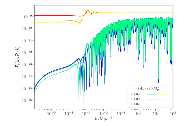
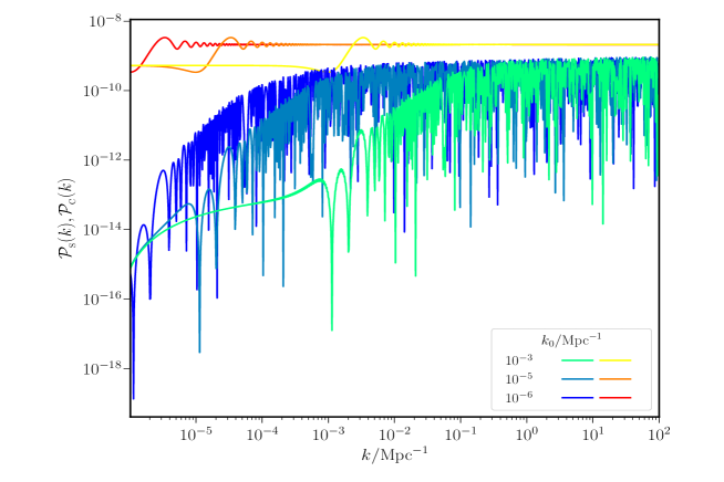
For discussing the results of this model, we shall consider the four parameters, namely, $V_{0}/M_{{}_{\mathrm{Pl}}}^{4}$, $(A_{-}/V_{0})M_{{}_{\mathrm{Pl}}}$, $\Delta A/A_{+}$ and $k_{0}/{\rm Mpc}^{-1}$. From Eq. (48), it is clear that $V_{0}/M_{{}_{\mathrm{Pl}}}^{4}$ and $(A_{-}/V_{0})M_{{}_{\mathrm{Pl}}}$ only affect the amplitude of $\mathcal{P}_{{}_{\mathrm{S}}}(k)$ which is already constrained by data to be about $2.1\times 10^{-9}$. The combination of parameters that dictate the prominence of features in $\mathcal{P}_{{}_{\mathrm{S}}}(k)$ is $\Delta A/A_{+}$, whereas $k_{0}$ decides the location of these features in the range of wavenumbers. On the other hand, $\mathcal{P}_{{}_{\mathrm{C}}}(k)$ is proportional not only to $V_{0}/M_{{}_{\mathrm{Pl}}}^{4}$ and $(A_{-}/V_{0})M_{{}_{\mathrm{Pl}}}$ like $\mathcal{P}_{{}_{\mathrm{S}}}(k)$, but also to $A_{-}/A_{+}$ and $k_{0}/k$. So, we can expect to see a large variation in $\mathcal{P}_{{}_{\mathrm{C}}}(k)$ just by changing the behaviour and location of oscillations in $\mathcal{P}_{{}_{\mathrm{S}}}(k)$. Thus, we shall explore variation in the values of $A_{+}$ and $k_{0}$ and study the effect on $\mathcal{P}_{{}_{\mathrm{S}}}(k)$, $\mathcal{P}_{{}_{\mathrm{C}}}(k)$ and $C_{\ell}$ .

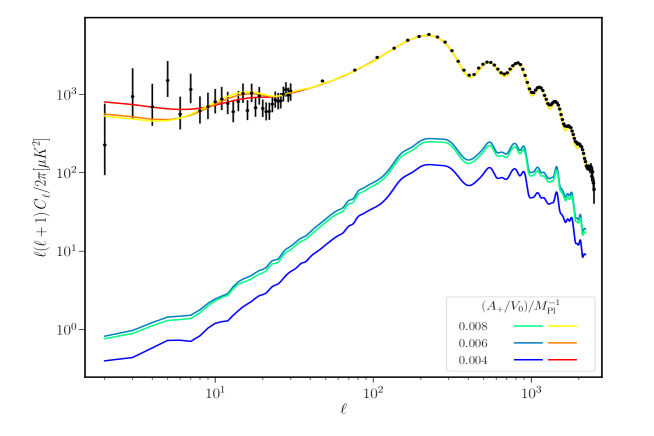
We present the effect of variation of $(A_{+}/V_{0})/M_{{}_{\mathrm{Pl}}}$ on $\mathcal{P}_{{}_{\mathrm{S}}}(k)$ and $\mathcal{P}_{{}_{\mathrm{C}}}(k)$ in Fig. 9. We fix the values of other model parameters to be $V_{0}/M_{{}_{\mathrm{Pl}}}^{4}=2.48\times 10^{-12}$, $(A_{-}/V_{0})/M_{{}_{\mathrm{Pl}}}^{-1}=3.14\times 10^{-3}$ and $k_{0}/\,{\rm Mpc}^{-1}=3.89\times 10^{-4}$. We note that the overall envelope of $\mathcal{P}_{{}_{\mathrm{C}}}(k)$ is dictated by $\ln(k_{\rm min}/k)$, as can be expected from our examination of local type $f_{{}_{\rm NL}}$ where regulating the divergence at $(x,y)=(0,1)$ lead to such a function in $\mathcal{P}_{{}_{\mathrm{C}}}(k)$. Further, the combination of terms that appear in the prefactor of $\mathcal{P}_{{}_{\mathrm{C}}}(k)$, $(A_{-}/A_{+})^{2}(1-A_{-}/A_{+})^{2}$, suggests that the amplitude shall be maximum at $A_{+}=2\,A_{-}$. We vary the value of $(A_{+}/V_{0})M_{{}_{\mathrm{Pl}}}$ around this range and find that the maximum of $\mathcal{P}_{{}_{\mathrm{C}}}(k)$ is indeed achieved at $(A_{+}/V_{0})M_{{}_{\mathrm{Pl}}}=6\times 10^{-3}\simeq 2(\,A_{-}/V_{0})M_{{}_{\mathrm{Pl}}}$. The corresponding CMB angular spectra are presented in Fig. 11. The standard spectra are computed for $\mathcal{P}_{{}_{\mathrm{S}}}(k)$ with the corresponding values of $(A_{+}/V_{0})M_{{}_{\mathrm{Pl}}}$. We find that the amplitude of $C_{\ell}$s due to $\mathcal{P}_{{}_{\mathrm{C}}}(k)$, though subdominant to $C_{\ell}$s due to $\mathcal{P}_{{}_{\mathrm{S}}}(k)$, may leave minor imprints on the latter as their amplitudes grow over small scales of around $\ell\geq 10^{3}$. Moreover, a crucial takeaway from this effect is that, the dependence of $\mathcal{P}_{{}_{\mathrm{C}}}(k)$ on $A_{+}$ and $A_{-}$, which is distinct from the factor $\Delta A/A_{+}$ as it appears in $\mathcal{P}_{{}_{\mathrm{S}}}(k)$, shall help resolve the degeneracy between $A_{+}$ and $A_{-}$ if compared against the data.

In Fig. 10, we illustrate the effect of varying $k_{0}/{\rm Mpc}^{-1}$. We fix $(A_{+}/V_{0})/M_{{}_{\mathrm{Pl}}}^{-1}=6.28\times 10^{-3}$ along with $V_{0}$ and $A_{-}$ as their values mentioned earlier. We infer that varying $k_{0}$ shifts the location of the onset of features in both $\mathcal{P}_{{}_{\mathrm{S}}}(k)$ and $\mathcal{P}_{{}_{\mathrm{C}}}(k)$. The oscillations over $k>k_{0}$ are particularly strong in $\mathcal{P}_{{}_{\mathrm{C}}}(k)$ and they settle at asymptotic values over $k\gg k_{0}$ essentially, due to the regulatory factor $1/[1+(k+kx+ky)/k_{\rm reg}]$ introduced in the bispectrum. Over $k\ll k_{0}$, we find that the $\mathcal{P}_{{}_{\mathrm{C}}}(k)$ tend to values independent of $k_{0}$. This can be understood as an indication that the integral in Eq. (60) evaluates to $(k/k_{0})^{2}$ over $k\ll k_{0}$ so that the term $(k_{0}/k)^{2}$ in the prefactor is cancelled, leaving $\mathcal{P}_{{}_{\mathrm{C}}}(k)$ independent of $k_{0}$. The overall envelope of $\mathcal{P}_{{}_{\mathrm{C}}}(k)$ is dictated by $\ln(k_{\rm min}/k)$ as seen before. The corresponding angular spectra are presented in Fig. 12. Surprisingly, we find that decrease in the value of $k_{0}$ leads to an increase in the amplitude of $C_{\ell}$s especially over large scales. However, this also pushes the feature of suppression in the original $C_{\ell}$s due to $\mathcal{P}_{{}_{\mathrm{S}}}(k)$ out of the observable window. This complementary behavior in the spectra where the amplitude of $C_{\ell}$s due $\mathcal{P}_{{}_{\mathrm{C}}}(k)$ is enhanced while feature in $C_{\ell}$s due $\mathcal{P}_{{}_{\mathrm{S}}}(k)$ is suppressed leads to an interesting case where, for $k_{0}/{\rm Mpc}^{-1}=10^{-6}$, the $C_{\ell}$s due $\mathcal{P}_{{}_{\mathrm{C}}}(k)$ acquire a magnitude of roughly about $10\%$ of the original $C_{\ell}$s due $\mathcal{P}_{{}_{\mathrm{S}}}(k)$.

In summary, in this model of Starobinsky, $C_{\ell}$s due to $\mathcal{P}_{{}_{\mathrm{C}}}(k)$ do not become comparable to the standard $C_{\ell}$s, for the range of values explored in $k_{0}$ and $A_{+}$. However, we see that the former may induce $1-10\%$ change in the latter for certain values of these parameters and lead to interesting effects, mainly because of the difference in the dependence of $\mathcal{P}_{{}_{\mathrm{C}}}(k)$ and $\mathcal{P}_{{}_{\mathrm{S}}}(k)$ on the model parameters. This is a compelling case to consider the contribution to $C_{\ell}$s due to $\mathcal{P}_{{}_{\mathrm{C}}}(k)$ in comparing this model against the data where the current constraints on $k_{0}$ may be altered and the degeneracy between $A_{-}$ and $A_{+}$ may be ameliorated due to the unique dependence of $\mathcal{P}_{{}_{\mathrm{C}}}(k)$ on them.

Figure 11: The angular spectra obtained from $\mathcal{P}_{{}_{\mathrm{S}}}(k)$ (in shades of red to yellow) and $\mathcal{P}_{{}_{\mathrm{C}}}(k)$ (in blue to green) are presented for the Starobinsky model across a range of the parameter $(A_{+}/V_{0})/M_{{}_{\mathrm{Pl}}}^{-1}$. We have set $k_{0}/\,{\rm Mpc}^{-1}=3.89\times 10^{-4}$, $V_{0}/M_{{}_{\mathrm{Pl}}}^{4}=2.48\times 10^{-12}$ and $(A_{-}/V_{0})/M_{{}_{\mathrm{Pl}}}^{-1}=3.14\times 10^{-3}$, in obtaining these plots. The oscillatory patterns are more pronounced in the spectra due to $\mathcal{P}_{{}_{\mathrm{S}}}(k)$ as we increase this parameter. The $C_{\ell}$s due to $\mathcal{P}_{{}_{\mathrm{C}}}(k)$ in general grow toward large $\ell$ values and the highest amplitude is achieved when $(A_{+}/V_{0})/M_{{}_{\mathrm{Pl}}}^{-1}$ is twice that of $(A_{-}/V_{0})/M_{{}_{\mathrm{Pl}}}^{-1}$.

Figure 12: The angular spectra derived from $\mathcal{P}_{{}_{\mathrm{S}}}(k)$ (in red to yellow) and $\mathcal{P}_{{}_{\mathrm{C}}}(k)$ (in blue to green) is presented for the Starobinsky model across a range of the parameter $k_{0}/\,{\rm Mpc}^{-1}$. We have set $V_{0}/M_{{}_{\mathrm{Pl}}}^{4}=2.48\times 10^{-12}$, $(A_{-}/V_{0})/M_{{}_{\mathrm{Pl}}}^{-1}=3.14\times 10^{-3}$ and $\Delta A/A_{+}=-0.5\Rightarrow(A_{+}/V_{0})/M_{{}_{\mathrm{Pl}}}^{-1}=6.28\times 10^{-3}$, in obtaining these plots. As $k_{0}$ is decreased, the oscillatory patterns shift toward small $\ell$ values in $C_{\ell}$s due to $\mathcal{P}_{{}_{\mathrm{S}}}(k)$. However, the amplitude of $C_{\ell}$s due to $\mathcal{P}_{{}_{\mathrm{C}}}(k)$ increases with decrease in $k_{0}$.

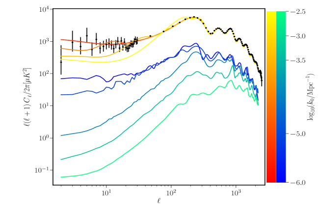
V Conclusion

This work examines a method of accounting non-Gaussian corrections to the primordial scalar power, arising at the level of scalar bispectrum through the associated non-Gaussianity parameter $f_{{}_{\rm NL}}(k_{1},k_{2},k_{3})$. We have computed the CMB angular spectra arising from such non-Gaussian corrections for various templates of $f_{{}_{\rm NL}}$ and for Starobinsky model. We have studied their dependence on various model parameters and determined the typical range of parameters that may lead to imprints on the standard angular spectrum. We have found that such an exercise can possibly alter the existing fitness of these models against the Planck dataset.

We have shown that this method provides an avenue to explore novel dependences on model parameters that are not captured in the original power spectrum of the Gaussian perturbations. This property is well observed in the cases of oscillatory template of power and bi-spectra and Starobinsky model. They can, in principle, break, or at least reduce, the degeneracies amongst parameters, which cannot be resolved at the level of $\mathcal{P}_{{}_{\mathrm{S}}}(k)$.

However, there are a few caveats and hence room for improvement in this analysis. Since we have focused on illustrating the major effects of $\mathcal{P}_{{}_{\mathrm{C}}}(k)$ on CMB, we have not completely computed the complicated integrals over ($x,y)$, that arise in various templates of $f_{{}_{\rm NL}}(k_{1},k_{2},k_{3})$. Since, they are of ${\cal O}(1)$, we have either worked with their maximum possible contribution or set them to unity to arrive at our results. As a future course of this work, we intend to carry out these integrals exactly, either analytically or numerically. Particularly, we shall focus on realistic models of inflation along the lines of Starobinsky model, and compute the complete $\mathcal{P}_{{}_{\mathrm{C}}}(k)$ arising from them. We shall account for the non-linear lensing, that has been neglected in this work, while studying the complete angular spectra due to $\mathcal{P}_{{}_{\mathrm{S}}}(k)+\mathcal{P}_{{}_{\mathrm{C}}}(k)$. More importantly, we plan to perform a proper Bayesian analysis of comparing the complete angular spectra arising from these models, against the latest dataset of Planck 2018, comprising of both temperature and polarization spectra. We intend to study the updated posteriors of the associated parameters and infer any improvement or worsening in the fit of certain promising models due to their non-Gaussianities [58, 5, 62]. We are presently working in this direction.

Furthermore, this method can be extended to compute non-Gaussian corrections to the scalar power due to other types of three-point correlations such as scalar-tensor-tensor and scalar-scalar-tensor types [63, 64]. It can be used to examine and constrain models with spectator fields that strongly interact with the scalar perturbations and thus giving rise to significant levels of non-Gaussianities [65, 66]. It can also be used to capture the effect of cross-correlation between scalar perturbations and gauge fields, in models of inflation that are considered in the context of primordial magnetogenesis [67, 68, 69]. In summary, the method presented in our work shall serve as an effective tool for examining and constraining a variety of non-Gaussianities arising in some of the non-trivial models of inflation.

Appendix A Behavior of integrands

The behaviors of integrands involved in arriving at $\mathcal{P}_{{}_{\mathrm{C}}}(k)$ arising in various templates and the model studied are presented and briefly discussed in this appendix. We plot the the density map of these integrand over a range of the variables of integration $x$ and $y$. Since the integrands typically decay rapidly as $1/(x^{2}y^{2})$, we focus on region around origin to study their shapes.

A.1 Local type

In case of local type $f_{{}_{\rm NL}}$, the integrand diverges at the two points of $(x,y)=(0,1)$ and $(1,0)$ due to the presence of $1/(xy)^{2}$ term. The computation of the double integrals using a finite value of $k_{\rm min}$ can be understood as follows. Using Eq. (8), we may obtain

$$\mathcal{P}_{{}_{\mathrm{C}}}(k) = \frac{9}{25}(f_{{}_{\rm NL}}^{\rm loc})^{2}\,A_{s}^{2}\,\left(\frac{k}{k_{\ast}}\right)^{2(n_{{}_{\mathrm{S}}}-1)}\int_{0}^{\infty}{\rm d}x\,x^{n_{{}_{\mathrm{S}}}-3}\int_{|1-x|}^{(1+x)}{\rm d}y\,y^{n_{{}_{\mathrm{S}}}-3}.$$ (61)

We shall ignore the minor effect of $x^{n_{{}_{\mathrm{S}}}-1}$ and $y^{n_{{}_{\mathrm{S}}}-1}$ within the integral and rewrite $\mathcal{P}_{{}_{\mathrm{C}}}(k)$ as

$$\mathcal{P}_{{}_{\mathrm{C}}}(k) = \frac{9}{25}(f_{{}_{\rm NL}}^{\rm loc})^{2}\mathcal{P}_{{}_{\mathrm{S}}}^{2}(k)\int_{0}^{\infty}{\rm d}x\,x^{-2}\int_{|1-x|}^{(1+x)}{\rm d}y\,y^{-2}$$ (62)

$$= -\frac{9}{25}(f_{{}_{\rm NL}}^{\rm loc})^{2}\mathcal{P}_{{}_{\mathrm{S}}}^{2}(k)\int_{0}^{\infty}{\rm d}x\,x^{-2}\left(\frac{1}{1+x}-\frac{1}{|1-x|}\right)$$

$$= -\frac{9}{25}(f_{{}_{\rm NL}}^{\rm loc})^{2}\mathcal{P}_{{}_{\mathrm{S}}}^{2}(k)\left\{\int_{0}^{1}{\rm d}x\,x^{-2}\left(\frac{1}{1+x}-\frac{1}{1-x}\right)+\int_{1}^{\infty}{\rm d}x\,x^{-2}\left(\frac{1}{1+x}+\frac{1}{1-x}\right)\right\}$$

$$= \frac{18}{25}(f_{{}_{\rm NL}}^{\rm loc})^{2}\mathcal{P}_{{}_{\mathrm{S}}}^{2}(k)\left\{\int_{0}^{1}{\rm d}x\,\frac{1}{x(1-x^{2})}+\int_{1}^{\infty}{\rm d}x\,\frac{1}{x^{2}(x^{2}-1)}\right\}$$

$$= \frac{18}{25}(f_{{}_{\rm NL}}^{\rm loc})^{2}\mathcal{P}_{{}_{\mathrm{S}}}^{2}(k)\lim_{x_{\rm min}\rightarrow 0}\left\{\ln{|1+x_{\rm min}|}-\frac{\ln{|(1+x_{\rm min})^{2}-1|}}{2}-\ln{|x_{\rm min}|}\right.$$

$$+\left.\frac{\ln{|x_{\rm min}^{2}-1|}}{2}+\frac{\ln{(2+x_{\rm min})}}{2}-\frac{1}{1+x_{\rm min}}-\frac{\ln{x_{\rm min}}}{2}\right\}$$

$$= \frac{18}{25}(f_{{}_{\rm NL}}^{\rm loc})^{2}\mathcal{P}_{{}_{\mathrm{S}}}^{2}(k)\lim_{x_{\rm min}\rightarrow 0}\left\{\frac{3\ln{(1+x_{\rm min})}}{2}-2\ln{x_{\rm min}}+\frac{\ln{(1-x_{\rm min})}}{2}-\frac{1}{1+x_{\rm min}}\right\}$$

$$= -\frac{18}{25}(f_{{}_{\rm NL}}^{\rm loc})^{2}\mathcal{P}_{{}_{\mathrm{S}}}^{2}(k)\left(1+2\lim_{x_{\rm min}\rightarrow 0}\ln{x_{\rm min}}\right).$$

The quantity $x_{\rm min}={k_{\rm min}}/{k}$ and so

$$\mathcal{P}_{{}_{\mathrm{C}}}(k) = -\frac{18}{25}(f_{{}_{\rm NL}}^{\rm loc})^{2}\mathcal{P}_{{}_{\mathrm{S}}}^{2}(k)\left(1+2\lim_{k_{\rm min}\rightarrow 0}\ln{\frac{k_{\rm min}}{k}}\right)\,.$$ (63)

Here and wherever such regulation is required, the value of $k_{\rm min}/\,{\rm Mpc}^{-1}$ is set to be $10^{-6}$ as mentioned in the main text. The shape of $\mathcal{P}_{{}_{\mathrm{C}}}(k)$ is hence detemined by $(k/k_{\ast})^{2(n_{{}_{\mathrm{S}}}-1)}$ in $\mathcal{P}_{{}_{\mathrm{S}}}(k)$ and $\ln(k_{\rm min}/k)$.

A.2 Orthogonal type

In case of orthogonal form of $f_{{}_{\rm NL}}(k_{1},k_{2},k_{3})$, the integrand that arises in calculating $\mathcal{P}_{{}_{\mathrm{C}}}(k)$ is sharply peaked along the line of $y=1-x$. This is depicted in Fig. 13. But the integrand does not diverge as it happens in the case of local type. So we focus in integrating over this region to capture the dominant contribution to $\mathcal{P}_{{}_{\mathrm{C}}}(k)$.

A.3 Equilateral type

In case of equilateral shape of $f_{{}_{\rm NL}}(k_{1},k_{2},k_{3})$, the integrand once again is well behaved without any divergences as plotted in Fig. 14. The amplitude is localized and of order unity around the region of $x=y=1$, and it rapidly decays down to smaller values away from this region. Hence, we perform integration over this region to obtain the magnitude of the contribution to $\mathcal{P}_{{}_{\mathrm{C}}}(k)$.

Figure 13: The integrand involved in $\mathcal{P}_{{}_{\mathrm{C}}}^{\rm ortho}(k)$ is plotted as a function of $x,y$. We have separated and accounted for the constants namely, $A_{{}_{\rm S}}$ and $f_{{}_{\rm NL}}^{\rm ortho}$ in $\mathcal{P}_{{}_{\mathrm{C}}}^{\rm ortho}(k)$ and plot here, only the part of function dependent on $x,y$. We find that the integrand peaks along $y=1-x$, with maximum at $x=y=1/2$ and falls rapidly for larger values of $x$ and $y$.

Figure 14: The integrand involved in $\mathcal{P}_{{}_{\mathrm{C}}}^{\rm eq}(k)$ is plotted as a function of $x,y$. As in the previous plot, we have already accounted for the constants like $A_{{}_{\rm S}}$ and $f_{{}_{\rm NL}}^{\rm eq}$. We find that the integrand has a maximum at $x=y=0.719$ and falls rapidly away from this region.

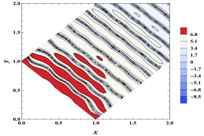
A.4 Oscillatory type

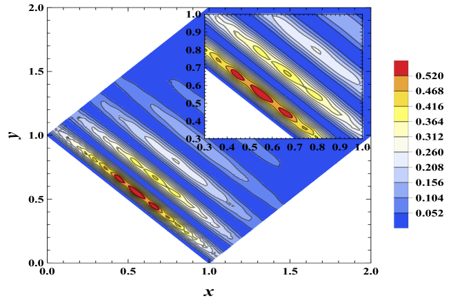
We present the integrand for the oscillatory template of $f_{{}_{\rm NL}}(k_{1},k_{2},k_{3})$ in Fig. 15. We see that the integrand exhibits oscillatory patterns along both $x$ and $y$ directions. There are no divergences present and further, it decays down in amplitude as $x$ and $y$ grow to large values. Note that the integrand plotted corresponds to the complete expression as described in Eq. (29). However, we have expanded this integral order by order in the parameter $b$ and extracted the scale dependence at each order in the main text. The associated integrals, denoted as $\cal I$ and ${\cal I}^{(b)}$, that arise at the level of ${\cal O}(b^{0})$ and ${\cal O}(b)$ respectively, are presented below.

Figure 15: The integrand involved in computing $\mathcal{P}_{{}_{\mathrm{C}}}^{\rm osc}(k)$ is plotted as a function of $x,y$. Note that we have plotted only the integrand involving $x,y$ excluding the numerical factors such as $A_{{}_{\rm S}}$, $f_{{}_{\rm NL}}^{\rm osc}$ [cf. Eq. (29)]. We have chosen other parameters to be $k=k_{\ast},\,k_{o}/\,{\rm Mpc}^{-1}=0.1$ and $b=0.05$. We have set $\omega=30$ to better illustrate the oscillatory patterns in $x$ as well as $y$ directions in the range presented. As can be expected, the quantity is positive throughout the range and unity at maximum. It peaks around $x=y=0.55$ and falls rapidly over large values of $x,y$ as can be seen in the inset.

Figure 16: The integrand involved in computing $\mathcal{P}_{{}_{\mathrm{C}}}(k)$ for Starobinsky model is plotted as a function of $x,y$, as a 2D projection on top and 3D plot below. We have plotted only the integrand involving $x,y$ excluding the numerical scaling factor that is $(V_{0}/M_{{}_{\mathrm{Pl}}}^{4})^{2}/[(A_{-}/V_{0})/M_{{}_{\mathrm{Pl}}}^{-1}]^{4}$ arising due to $\mathcal{P}_{{}_{\mathrm{S}}}(kx),\,\mathcal{P}_{{}_{\mathrm{S}}}(ky)$. We have chosen parameters to be $k=k_{\ast},k_{o}/\,{\rm Mpc}^{-1}=4\times 10^{-3}$,$V_{0}/M_{{}_{\mathrm{Pl}}}^{4}=2.48\times 10^{-12}$ and $(A_{-}/V_{0})/M_{{}_{\mathrm{Pl}}}^{-1}=3.14\times 10^{-3}$ and $\Delta A/A_{+}=-0.5$. We have plotted the integrand in natural log to better illustrate the complex oscillations in $x$ as well as $y$ directions in the range presented. We find that it diverges at $(x,y)=\{(0,1),(1,0)\}$ and falls rapidly over large values of $x,y$ as seen in the 3D plot below.

The integrals involved in the expression of $\mathcal{P}_{{}_{\mathrm{C}}}^{\rm osc}(k)$ at the level of ${\cal O}(b^{0})$ are [cf. Eq. (32)]

$${\cal I}_{1} = \int_{0}^{\infty}{\rm d}x\int^{1+x}_{|1-x|}{\rm d}y\,\frac{1}{(1+x^{3}+y^{3})^{2}}\,,$$ (64)

$${\cal I}_{2} = \int_{0}^{\infty}{\rm d}x\int^{1+x}_{|1-x|}{\rm d}y\,\frac{\cos[2\omega\ln(1+x+y)]}{(1+x^{3}+y^{3})^{2}}\,,$$ (65)

$${\cal I}_{3} = \int_{0}^{\infty}{\rm d}x\int^{1+x}_{|1-x|}{\rm d}y\,\frac{\sin[2\omega\ln(1+x+y)]}{(1+x^{3}+y^{3})^{2}}\,.$$ (66)

The integrals required in computation of $\mathcal{P}_{{}_{\mathrm{C}}}^{\rm osc}(k)$ at the level of ${\cal O}(b)$ are [cf. Eq. (35)]

$${\cal I}^{(b)}_{1} = \int^{\infty}_{0}{\rm d}x\int^{1+x}_{|1-x|}{\rm d}y\cos^{2}\left[\omega\ln(1+x+y)\right]\,\frac{f_{1}(x,y)}{(1+x^{3}+y^{3})^{3}}\,,$$ (67)

$${\cal I}^{(b)}_{2} = \int^{\infty}_{0}{\rm d}x\int^{1+x}_{|1-x|}{\rm d}y\cos^{2}\left[\omega\ln(1+x+y)\right]\,\frac{f_{2}(x,y)}{(1+x^{3}+y^{3})^{3}}\,,$$ (68)

$${\cal I}^{(b)}_{3} = \int^{\infty}_{0}{\rm d}x\int^{1+x}_{|1-x|}{\rm d}y\sin^{2}\left[\omega\ln(1+x+y)\right]\,\frac{f_{1}(x,y)}{(1+x^{3}+y^{3})^{3}}\,,$$ (69)

$${\cal I}^{(b)}_{4} = \int^{\infty}_{0}{\rm d}x\int^{1+x}_{|1-x|}{\rm d}y\sin^{2}\left[\omega\ln(1+x+y)\right]\,\frac{f_{2}(x,y)}{(1+x^{3}+y^{3})^{3}}\,,$$ (70)

$${\cal I}^{(b)}_{5} = \int^{\infty}_{0}{\rm d}x\int^{1+x}_{|1-x|}{\rm d}y\sin 2\left[\omega\ln(1+x+y)\right]\,\frac{f_{1}(x,y)}{(1+x^{3}+y^{3})^{3}}\,,$$ (71)

$${\cal I}^{(b)}_{6} = \int^{\infty}_{0}{\rm d}x\int^{1+x}_{|1-x|}{\rm d}y\sin 2\left[\omega\ln(1+x+y)\right]\,\frac{f_{2}(x,y)}{(1+x^{3}+y^{3})^{3}}\,,$$ (72)

where the functions $f_{1}(x,y)$ and $f_{2}(x,y)$ are given by

$$f_{1}(x,y) = x^{3}+y^{3}+(1+x^{3})\cos[\omega\ln y]+(1+y^{3})\cos[\omega\ln x]\,,$$ (73)

$$f_{2}(x,y) = (1+x^{3})\sin[\omega\ln y]+(1+y^{3})\sin[\omega\ln x]\,.$$ (74)

The integrands of these integrals and hence the integrals themselves evaluate to ${\cal O}(1)$ and hence are assumed to be unity in illustration of $\mathcal{P}_{{}_{\mathrm{C}}}^{\rm osc}(k)$ and the associated $C_{\ell}$s.

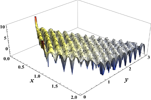
A.5 Starobinsky model

The integrand involved in calculation of $\mathcal{P}_{{}_{\mathrm{C}}}(k)$ for Starobinsky model is presented in Fig. 16. We see that it has a highly non-trivial oscillatory feature throughout the range of integration. There are divergences at $(x,y)=(0,1)$ and $(1,0)$ as was the case for local type. Moreover, there is a decay of amplitude as $x$ and $y$ tend toward large values. We have also presented the same integrand in a 3D plot, projected at an angle, to better illustrate its nature. The complicated shape of the integrand does not allow for any approximate evaluation of the integral and hence we perform the integration numerically.

References

- Contaldi et al. [2003] C. R. Contaldi, M. Peloso, L. Kofman, and A. D. Linde, JCAP 07, 002, arXiv:astro-ph/0303636 .
- Sinha and Souradeep [2006] R. Sinha and T. Souradeep, Phys. Rev. D 74, 043518 (2006), arXiv:astro-ph/0511808 .
- Hazra et al. [2013a] D. K. Hazra, A. Shafieloo, and G. F. Smoot, JCAP 12, 035, arXiv:1310.3038 [astro-ph.CO] .
- Meerburg and Spergel [2014] P. D. Meerburg and D. N. Spergel, Phys. Rev. D 89, 063537 (2014), arXiv:1308.3705 [astro-ph.CO] .
- Ragavendra et al. [2022] H. V. Ragavendra, D. Chowdhury, and L. Sriramkumar, Phys. Rev. D 106, 043535 (2022), arXiv:2003.01099 [astro-ph.CO] .
- Sohn et al. [2022] W. Sohn, A. Shafieloo, and D. K. Hazra, (2022), arXiv:2211.15139 [astro-ph.CO] .
- Braglia et al. [2023] M. Braglia, X. Chen, D. K. Hazra, and L. Pinol, JCAP 03, 014, arXiv:2210.07028 [astro-ph.CO] .
- Ade et al. [2016] P. Ade et al. (Planck), Astron. Astrophys. 594, A20 (2016), arXiv:1502.02114 [astro-ph.CO] .
- Akrami et al. [2020a] Y. Akrami et al. (Planck), Astron. Astrophys. 641, A10 (2020a), arXiv:1807.06211 [astro-ph.CO] .
- Chen et al. [2008] X. Chen, R. Easther, and E. A. Lim, JCAP 04, 010, arXiv:0801.3295 [astro-ph] .
- Martin and Sriramkumar [2012] J. Martin and L. Sriramkumar, JCAP 01, 008, arXiv:1109.5838 [astro-ph.CO] .
- Adshead et al. [2012] P. Adshead, C. Dvorkin, W. Hu, and E. A. Lim, Phys. Rev. D 85, 023531 (2012), arXiv:1110.3050 [astro-ph.CO] .
- Hazra et al. [2013b] D. K. Hazra, L. Sriramkumar, and J. Martin, JCAP 05, 026, arXiv:1201.0926 [astro-ph.CO] .
- Basu et al. [2019] S. Basu, D. J. Brooker, N. C. Tsamis, and R. P. Woodard, Phys. Rev. D 100, 063525 (2019), arXiv:1905.12140 [gr-qc] .
- Ragavendra et al. [2020] H. V. Ragavendra, D. Chowdhury, and L. Sriramkumar, Springer Proc. Phys. 248, 39 (2020), arXiv:1906.03942 [astro-ph.CO] .
- Clarke and Shellard [2021] P. Clarke and E. P. S. Shellard, JCAP 08, 002, arXiv:2012.08546 [astro-ph.CO] .
- Ragavendra and Sriramkumar [2023] H. V. Ragavendra and L. Sriramkumar, Galaxies 11, 34 (2023), arXiv:2301.08887 [astro-ph.CO] .
- Babich et al. [2004] D. Babich, P. Creminelli, and M. Zaldarriaga, JCAP 08, 009, arXiv:astro-ph/0405356 .
- Bartolo et al. [2004] N. Bartolo, E. Komatsu, S. Matarrese, and A. Riotto, Phys. Rept. 402, 103 (2004), arXiv:astro-ph/0406398 .
- Creminelli et al. [2006] P. Creminelli, A. Nicolis, L. Senatore, M. Tegmark, and M. Zaldarriaga, JCAP 05, 004, arXiv:astro-ph/0509029 .
- Komatsu [2010] E. Komatsu, Class. Quant. Grav. 27, 124010 (2010), arXiv:1003.6097 [astro-ph.CO] .
- Akrami et al. [2020b] Y. Akrami et al. (Planck), Astron. Astrophys. 641, A9 (2020b), arXiv:1905.05697 [astro-ph.CO] .
- Ragavendra et al. [2021a] H. V. Ragavendra, P. Saha, L. Sriramkumar, and J. Silk, Phys. Rev. D 103, 083510 (2021a), arXiv:2008.12202 [astro-ph.CO] .
- Ragavendra et al. [2021b] H. V. Ragavendra, L. Sriramkumar, and J. Silk, JCAP 05, 010, arXiv:2011.09938 [astro-ph.CO] .
- Sloth [2006] M. S. Sloth, Nucl. Phys. B 748, 149 (2006), arXiv:astro-ph/0604488 .
- Byrnes et al. [2007] C. T. Byrnes, K. Koyama, M. Sasaki, and D. Wands, JCAP 11, 027, arXiv:0705.4096 [hep-th] .
- Cogollo et al. [2008] H. R. S. Cogollo, Y. Rodriguez, and C. A. Valenzuela-Toledo, JCAP 08, 029, arXiv:0806.1546 [astro-ph] .
- Dimastrogiovanni and Bartolo [2008] E. Dimastrogiovanni and N. Bartolo, JCAP 11, 016, arXiv:0807.2790 [astro-ph] .
- Senatore and Zaldarriaga [2010] L. Senatore and M. Zaldarriaga, JHEP 12, 008, arXiv:0912.2734 [hep-th] .
- Kristiano and Yokoyama [2022a] J. Kristiano and J. Yokoyama, Phys. Rev. Lett. 128, 061301 (2022a), arXiv:2104.01953 [hep-th] .
- Kristiano and Yokoyama [2022b] J. Kristiano and J. Yokoyama, (2022b), arXiv:2211.03395 [hep-th] .
- Riotto [2023] A. Riotto, (2023), arXiv:2301.00599 [astro-ph.CO] .
- Kristiano and Yokoyama [2023] J. Kristiano and J. Yokoyama, (2023), arXiv:2303.00341 [hep-th] .
- Choudhury et al. [2023] S. Choudhury, S. Panda, and M. Sami, (2023), arXiv:2303.06066 [astro-ph.CO] .
- Firouzjahi [2023] H. Firouzjahi, (2023), arXiv:2303.12025 [astro-ph.CO] .
- Ota et al. [2022] A. Ota, M. Sasaki, and Y. Wang, (2022), arXiv:2211.12766 [astro-ph.CO] .
- Yamauchi [2022] D. Yamauchi, PTEP 2022, 073E02 (2022), arXiv:2203.15599 [astro-ph.CO] .
- Cai et al. [2019a] R.-g. Cai, S. Pi, and M. Sasaki, Phys. Rev. Lett. 122, 201101 (2019a), arXiv:1810.11000 [astro-ph.CO] .
- Unal [2019] C. Unal, Phys. Rev. D 99, 041301 (2019), arXiv:1811.09151 [astro-ph.CO] .
- Cai et al. [2019b] R.-G. Cai, S. Pi, S.-J. Wang, and X.-Y. Yang, JCAP 05, 013, arXiv:1901.10152 [astro-ph.CO] .
- Adshead et al. [2021] P. Adshead, K. D. Lozanov, and Z. J. Weiner, (2021), arXiv:2105.01659 [astro-ph.CO] .
- Ragavendra [2022] H. V. Ragavendra, Phys. Rev. D 105, 063533 (2022), arXiv:2108.04193 [astro-ph.CO] .
- Chen et al. [2022a] C. Chen, A. Ota, H.-Y. Zhu, and Y. Zhu, (2022a), arXiv:2210.17176 [astro-ph.CO] .
- Schmidt and Kamionkowski [2010] F. Schmidt and M. Kamionkowski, Phys. Rev. D 82, 103002 (2010), arXiv:1008.0638 [astro-ph.CO] .
- Agullo et al. [2021] I. Agullo, D. Kranas, and V. Sreenath, Front. Astron. Space Sci. 8, 703845 (2021), arXiv:2105.12993 [gr-qc] .
- Maldacena [2003] J. M. Maldacena, JHEP 05, 013, arXiv:astro-ph/0210603 .
- Seery [2010] D. Seery, Class. Quant. Grav. 27, 124005 (2010), arXiv:1005.1649 [astro-ph.CO] .
- Gerstenlauer et al. [2011] M. Gerstenlauer, A. Hebecker, and G. Tasinato, JCAP 06, 021, arXiv:1102.0560 [astro-ph.CO] .
- Lewis et al. [2000] A. Lewis, A. Challinor, and A. Lasenby, Astrophys. J. 538, 473 (2000), arXiv:astro-ph/9911177 .
- Jung and van Tent [2017] G. Jung and B. van Tent, JCAP 05, 019, arXiv:1611.09233 [astro-ph.CO] .
- Atal and Germani [2019] V. Atal and C. Germani, Phys. Dark Univ. 24, 100275 (2019), arXiv:1811.07857 [astro-ph.CO] .
- Meerburg et al. [2009] P. D. Meerburg, J. P. van der Schaar, and P. S. Corasaniti, JCAP 05, 018, arXiv:0901.4044 [hep-th] .
- Brandenberger and Martin [2013] R. H. Brandenberger and J. Martin, Class. Quant. Grav. 30, 113001 (2013), arXiv:1211.6753 [astro-ph.CO] .
- Oppizzi et al. [2018] F. Oppizzi, M. Liguori, A. Renzi, F. Arroja, and N. Bartolo, JCAP 05, 045, arXiv:1711.08286 [astro-ph.CO] .
- Flauger and Pajer [2011] R. Flauger and E. Pajer, JCAP 01, 017, arXiv:1002.0833 [hep-th] .
- Sreenath et al. [2015] V. Sreenath, D. K. Hazra, and L. Sriramkumar, JCAP 02, 029, arXiv:1410.0252 [astro-ph.CO] .
- Flauger et al. [2010] R. Flauger, L. McAllister, E. Pajer, A. Westphal, and G. Xu, JCAP 06, 009, arXiv:0907.2916 [hep-th] .
- Hazra et al. [2014] D. K. Hazra, A. Shafieloo, G. F. Smoot, and A. A. Starobinsky, JCAP 08, 048, arXiv:1405.2012 [astro-ph.CO] .
- Starobinsky [1992] A. A. Starobinsky, JETP Lett. 55, 489 (1992).
- Martin et al. [2014] J. Martin, L. Sriramkumar, and D. K. Hazra, JCAP 09, 039, arXiv:1404.6093 [astro-ph.CO] .
- Arroja and Tanaka [2011] F. Arroja and T. Tanaka, JCAP 05, 005, arXiv:1103.1102 [astro-ph.CO] .
- Antony et al. [2023] A. Antony, F. Finelli, D. K. Hazra, and A. Shafieloo, Phys. Rev. Lett. 130, 111001 (2023), arXiv:2202.14028 [astro-ph.CO] .
- Sreenath et al. [2013] V. Sreenath, R. Tibrewala, and L. Sriramkumar, JCAP 12, 037, arXiv:1309.7169 [astro-ph.CO] .
- Chowdhury et al. [2016] D. Chowdhury, V. Sreenath, and L. Sriramkumar, JCAP 11, 041, arXiv:1605.05292 [astro-ph.CO] .
- Wang et al. [2022] L.-T. Wang, Z.-Z. Xianyu, and Y.-M. Zhong, JHEP 02, 085, arXiv:2109.14635 [hep-ph] .
- Chen et al. [2022b] X. Chen, R. Ebadi, and S. Kumar, JCAP 08, 083, arXiv:2205.01107 [hep-ph] .
- Chowdhury et al. [2018] D. Chowdhury, L. Sriramkumar, and M. Kamionkowski, JCAP 10, 031, arXiv:1807.07477 [astro-ph.CO] .
- Tripathy et al. [2022] S. Tripathy, D. Chowdhury, R. K. Jain, and L. Sriramkumar, Phys. Rev. D 105, 063519 (2022), arXiv:2111.01478 [astro-ph.CO] .
- Tripathy et al. [2023] S. Tripathy, D. Chowdhury, H. V. Ragavendra, R. K. Jain, and L. Sriramkumar, Phys. Rev. D 107, 043501 (2023), arXiv:2211.05834 [astro-ph.CO] .