On the temporal tweezing of cavity solitons

Abstract

Motivated by the work of J.K. Jang et al., Nat. Commun.  6, 7370 (2015), where the authors experimentally tweeze cavity solitons in a passive loop of optical fiber, we study the amenability to tweezing of cavity solitons as the properties of a localized tweezer are varied. The system is modeled by the Lugiato-Lefever equation, a variant of the complex Ginzburg-Landau equation. We produced an effective, localized, trapping tweezer potential by assuming a Gaussian phase-modulation of the holding beam. The potential for tweezing is then assessed as the width, the total (temporal) displacement and speed of the tweezer are varied and corresponding phase diagrams are presented. As the relative speed of the tweezer is increased we find four possible dynamical scenarios: (a) successful tweezing, (b) release and recapture, (c) destruction due to absorption, and (d) release without recapture of the cavity soliton. We also deploy a non-conservative variational approximation (NCVA) based on a Lagrangian description which reduces the original no-Hamiltonian partial differential equation to a set of coupled ordinary differential equations on the cavity soliton parameters. We show how the NCVA is capable of predicting the threshold in the tweezer parameters for successful tweezing. Through the numerical study of the Lugiato-Lefever equation and its NCVA reduction, we have developed a process to identify regions of successful tweezing which can aid in the experimental design and reliability of temporal tweezing used for information processing.

Acknowledgments

R.C.G. gratefully acknowledges support from the US National Science Foundation under Grants PHY-1603058 and PHY-2110038. P.G.K. gratefully acknowledges support from the US National Science Foundation under Grants DMS-2204702 and PHY-2110030.

1 Introduction

An optical tweezer, i.e., a single-beam gradient force trap, can trap, manipulate and move nanometer and micron-sized dielectric particles in space using a highly focused laser beam [1, 2]. Optical tweezers have been used in physics and biology to manipulate objects and measure forces [3]. The optical trapping and manipulation of the temporal position of light pulses is highly desirable as it may have direct implications for optical information processing. In this case, information is treated as a sequence of pulses that can be stored and reconfigured by trapping ultrashort pulses of light and dynamically moving them around in time. In particular, a temporal tweezer can exert similar control over ultrashort light pulses in time as reported in Ref. [4]. The optical trapping and manipulation of light pulses is useful in optical information processing [5, 6, 7, 8] where the information is represented as a sequence of pulses. Temporal tweezing is an effective method to trap ultrashort pulses of light and move them around in time in order to store and reconfigure the information. Optical information processing is partly achieved in slow-light [9, 10, 11, 12] and nonlinear cross-phase modulation effects [13, 14, 15, 16, 17, 18], however neither approach allows for the independent control of light pulses within the sequence. It should be noted that in the context of solitary waves transfer in continuum and discrete (gain and loss) media has been previously illustrated in Ref. [19], while the use of potentials (such as time-dependent optical [20, 21] or Bessel [22] lattices) has been used to drive solitary waves in atomic and optical systems. Such ideas of capture, release and overall control of the solitary waves have been popular in other areas too, including, e.g., in electrical lattice experiments [23]. Based on Ref. [4], we present an exhaustive analysis of temporal tweezing by means of direct numerical simulations as well as an analytical reduction based on a non-conservative variational approach (NCVA) [24].

We investigate temporal tweezing of cavity solitons in a passive loop of optical fiber pumped by a continuous-wave laser beam which is described by a modified Lugiato-Lefever (LL) partial differential equation (PDE) model which, in turn, is a special case of the celebrated complex Ginzburg-Landau equation [25, 26]. In the experiments described in Ref. [4], temporal cavity solitons (CSs) were created as picosecond pulses of light that recirculate in a loop of optical fiber and are exposed to temporal controls in the form of a gigahertz phase modulation. It has been shown, both theoretically and experimentally, that the CSs are attracted and trapped to phase maxima, suppressing all soliton interactions. These trapped CSs can then be manipulated in time, either forward or backward, which is known as temporal tweezing. We study the existence and dynamics of temporally tweezed CSs. The key phenomena reported herein are parametric regions separating the following tweezing scenarios: (i) successful temporal tweezing of the CS where the CS moves as prescribed by the tweezer, (ii) “dissipative” CSs where the CS is partially trapped but eventually dissipates away, and (iii) the effective potential moves too fast and leaves the CS behind. We also apply the NCVA to reduce the LL dynamics of CSs to a set of ordinary differential equations (ODEs) on the CSs parameter. We therefore, identify regions of temporal tweezing, and compare to the full numerical solutions of the original LL PDE.

The manuscript is organized as follows. In Sec 2 we introduce the temporal tweezing approach suggested in Ref. [4] and decribe the LL model. In Sec. 2.2 we add a Gaussian phase-modulation to the LL model and simulate the moving and manipulation of the CS. In Sec. 3 we provide a brief description of the NCVA approach and its formulation within the LL model. Then, the rest of the section is devoted to the application of the NCVA to capture the tweezing of a CS. In Sec. 4 we identify parameter regimes for the existence of trapped CSs and follow the tweezing dynamics from the ensuing manipulation of the phase-modulation of a continuous-wave holding beam. Finally, in Sec 5 we summarize our key findings and provide possible avenues for future research.

2 The Full Model: Lugiato-Lefever Equation and Temporal Phase Modulation

In our analysis of temporal tweezing we begin with dissipative solitons in externally-driven nonlinear passive cavities, the so-called temporal CSs [27, 28, 29, 30, 31, 32]. In a passive loop of optical fiber these light pulses can persist without losing shape because the dispersive temporal spreading is balanced by the material nonlinearity. Also, CSs persist without losing their intensity by drawing power from a continuous-wave (cw) “holding” laser beam driving the cavity. Multiple CSs may be simultaneously present in the optical loop and positioned independently temporally [33]. Here, we report on the trapping of CSs and the dynamical manipulation through selectively altering the phase profile of the holding beam.

2.1 Theory of Temporal Tweezing

Temporal tweezing requires a CS with an attractive time-domain drift towards the maxima of the intracavity phase profile. The attraction is due to the CSs shifting their instantaneous frequencies in response to a phase modulation. The gain and loss mechanisms inherent to this system may be captured by a variant of the celebrated complex Ginzburg-Landau (cGL) equation [25, 26]. In particular, following Refs. [4, 34, 35], we will model the system under consideration by the following Lugiato-Lefever (LL) equation:

$$z_{R}\frac{\partial E}{\partial z}=\left[-\alpha-i\delta_{0}-iL\frac{\beta_{2}}{2}\frac{\partial^{2}}{\partial\tau^{2}}+i\gamma L|E|^{2}\right]E+\sqrt{\theta}E_{\rm in},$$ (1)

where $z$ is the slow time describing the intracavity field envelope $E(z,\tau)$ and $\tau$ is the fast time describing the temporal profile of the field envelope in a reference frame traveling at the group velocity of the holding beam in the cavity. The cavity roundtrip time is $z_{R}$ and the field of the holding beam is $E_{\rm in}$ with power $P_{\rm in}=|E_{\rm in}|^{2}$. The cavity losses are accounted by $\alpha=\pi/\mathscr{F}$, where $\mathscr{F}$ is the cavity finesse. The phase detuning of the intracavity field to the closest cavity resonance of order $l$ is given by $\delta_{0}=2\pi l-\phi_{0}$ where $\phi_{0}$ is a linear phase-shift over one roundtrip with respect to the holding beam. Finally, $L$ is the cavity length, $\beta_{2}$ is the dispersion coefficient of the fiber, $\gamma$ is the nonlinear coefficient of the fiber, and $\theta$ is the input coupler power transmission coefficient.

In what follows, for ease of exposition, we will work in adimensional units. For that purpose, the LL Eq. (1) may be adimensionalized by introducing a dimensionless slow time $z^{\prime}=\alpha z/z_{R}$ and a dimensionless fast time $\tau^{\prime}=\tau\sqrt{2\alpha/(L|\beta_{2}|)}$. We also use a dimensionless complex field amplitude $v(z^{\prime},\tau^{\prime})=E(z,\tau)\sqrt{\gamma L/\alpha}$ and a dimensionless holding beam $v_{\rm in}=E_{\rm in}\sqrt{\gamma L\theta/\alpha^{3}}$. For convenience, we drop the primes in the notation of $z^{\prime}$ and $\tau^{\prime}$, such that Eq. (1) becomes the dimensionless mean-field LL equation

$$\frac{\partial v}{\partial z}=-(1+i\Delta)v+i|v|^{2}v+i\frac{\partial^{2}v}{\partial\tau^{2}}+v_{\rm in},$$ (2)

where $\Delta=\delta/\alpha$ is the effective dimensionless detuning.

Homogeneous and steady ($\tau$- and $z$-independent) states, $v(z,\tau)=v_{s}$, of Eq. (2), where the CSs will be supported, satisfy

$$|v_{s}|^{2}v_{s}=-iv_{s}+\Delta v_{s}+iv_{\rm in},$$ (3)

which may be cast in the form of a well-known cubic equation for dispersive optical bistability [36, 34, 6, 37]

$$I_{s}^{3}-2\Delta I_{s}^{2}+(1+\Delta^{2})I_{s}=I_{0},$$ (4)

where $I_{s}=|v_{s}|^{2}$ is the intracavity background field intensity and $I_{0}=|v_{\rm in}|^{2}$ is the holding beam intensity. Therefore, we obtain a steady state (implicit) solution

$$v_{s}=\frac{v_{\rm in}}{1+i(\Delta-I_{s})},$$

dependent on the detuning $\Delta$ and holding beam power $v_{\rm in}$. For small detuning, $\Delta<\sqrt{3}$, Eq. (4) has only one solution for the the steady state $I_{s}$ given a specific holding beam power $v_{\rm in}$. For large detuning, $\Delta>\sqrt{3}$, there are three solutions for $I_{s}$ given a specific holding beam power $v_{\rm in}$. The homogeneous solution is bistable since two solutions are stable while the other solution is unstable. The transition between the states occurs through a pitchfork bifurcation.

We follow the approach of Refs. [4, 38] to study the effect of phase-modulation of the holding field. The phase-modulation is imprinted into a constant holding beam which creates an effective potential necessary to attract, trap, and manipulate a CS. We assume a phase-modulation temporal profile $\phi(\tau)$ and rewrite the holding beam using

$$v_{\rm in}(\tau)=u_{\rm in}\exp[i\phi(\tau)],$$ (5)

where $u_{\rm in}$ is a constant scalar (whose square corresponds to the intensity of the holding beam). Substituting Eq. (5) into Eq. (2) with the ansatz $v(z,\tau)=u(z,\tau)\exp[i\phi(\tau)]$ yields

$$iu_{z}+|u|^{2}u+u_{\tau\tau}- (\Delta+(\phi^{\prime})^{2})u+2iu_{\tau}\phi^{\prime}=-i(1+\phi^{\prime\prime})u+iu_{\rm in},$$ (6)

where primes denote derivatives with respect to $\tau$. The cw intracavity field on which the CSs are supported has the same phase modulation as that imposed on the external holding beam in this non-dimensional form. In this form, the phase modulation of the holding beam introduces the following terms affecting then dynamics of the field envelope: (i) $(\phi^{\prime})^{2}$ acts like an effective potential caused by the phase modulation, (ii) the term $2iu_{\tau}\phi^{\prime}$ describes the effect of drift through the gradient term $u_{\tau}$ where $2\phi^{\prime}$ is the drift speed [39], and (iii) the $\phi^{\prime\prime}$ term induces an additional loss in the system caused by the phase modulation.

Steady state solutions of the LL Eq. (6) are subject to an additional constraint stemming from the balance condition $dP/dz=0$, where

$$P=\int_{-\infty}^{\infty}|u|^{2}d\tau,$$

is the total power (mathematically, the squared $L^{2}$ norm) of the cavity solitons. The evolution of $P$ can be found by multiplying Eq. (6) by $u^{*}$, the complex conjugate of Eq. (6) by $u$, and then adding and integrating the resulting equations [40]. For the LL Eq. (6), it is straightforward to find the following constraint condition for a steady state solution:

$$\int_{-\infty}^{\infty}\Big{(}-(1+\phi^{\prime\prime})|u|^{2}-\phi^{\prime}\left(u_{\tau}u^{*}+u_{\tau}^{*}u\right)+\mathrm{Re}(u)u_{\rm in}\Big{)}d\tau=0.$$ (7)

This power-balance constraint will need to be enforced in the system, and, in turn, will fix the cavity detuning $\Delta$ for a given set of parameters describing the phase modulation $\phi(\tau)$.

2.2 Tweezing of Cavity Solitons

Our analysis involves temporal cavity solitons described by LL Eq. (6) stored in a passive loop of optical fiber pumped by a cw laser beam. The CS is trapped into a specific time slot through phase-modulation of the holding beam, and moved around in time by manipulating the phase profile. Experimentally, a modulator imprints a time-varying electric signal $\phi(\tau)$ into the phase of the cw holding laser driving the cavity. For the purpose of the LL Eq. (6), we used a “natural” localized phase modulation with a Gaussian profile of the form

$$\phi(\tau)=h_{\phi}\exp\left[-\frac{(\tau-\tau_{0})^{2}}{2\sigma_{\phi}^{2}}\right],$$ (8)

where $h_{\phi}$, $\sigma_{\phi}$, and $\tau_{0}$ describe, respectively, the height, width, and center position of the phase profile.

In what follows, we will first consider the stationary solutions of the LL model in the form $u(z,\tau)=u_{0}(\tau)$ which are governed by the following ODE:

$$u_{0}^{\prime\prime}+\left(|u_{0}|^{2}-\Delta-(\phi^{\prime})^{2}\right)u_{0}+2i\phi^{\prime}u_{0}^{\prime\prime}=-i(1+\phi^{\prime\prime})u_{0}+iu_{\rm in},$$ (9)

It is important to recall that the stationary state (9) needs to be supplemented with the additional power-balance constraint (7) which needs to be enforced for the stationary solutions as follows:

$$\int_{-\infty}^{\infty}\Big{[}-(1+\phi^{\prime\prime})|u_{0}|^{2}-\phi^{\prime}\left(u_{0}^{\prime}u_{0}^{*}+{u_{0}^{*}}^{\prime}u_{0}\right)+\mathrm{Re}(u_{0})u_{\rm in}\Big{]}d\tau=0.$$ (10)

This self-consistency condition selects the particular value of the detuning $\Delta$ once the other parameters (i.e., $u_{\rm in}$, $h_{\phi}$, and $\sigma_{\phi}$) are fixed. Indeed, this parameter is reminiscent of the frequency of the solitary waves in the corresponding Hamiltonian, nonlinear Schrödinger (NLS) type settings [41]. While in such NLS systems, this parameter has freely tunable ranges, in the present dissipative system, it is determined by the relevant balance condition discussed above. Once stationary soliton solutions of the resulting differential-algebraic system of Eqs. (9) and (10) are identified at $\tau_{0}=0$, their “tweezability” (i.e., amenability to transfer via tweezers) is considered by measuring the amount of soliton intensity that remains inside and outside of the effective potential $(\phi^{\prime})^{2}$ as the center location of the tweezer is manipulated.

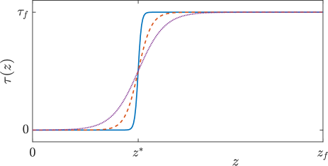
Figure 1: “Trajectory” of the temporal tweezing. The tweezer starts at $\tau=0$ and ends at $\tau=\tau_{f}$. The degree of adiabaticity is controlled with the parameter $\beta$ in Eq. (11). The solid (blue) line represent a fast transition (relatively large $\beta$) which will be unlikely to tweeze the CS. With higher degrees of adiabaticity (i.e., smaller values of $\beta$), see dashed and dotted curves, it will be more likely for the tweezing to be successful.

To simulate moving and manipulating the cavity soliton through the phase profile we consider the following “motion” in the evolution variable:

$$\tau_{0}(z)=\frac{\tau_{f}}{2}\left[\frac{\tanh[\beta(z-z^{*})]}{\tanh(\beta z^{*})}+1\right],$$ (11)

where $\tau_{f}$ is the final fast time $\tau$ at which the phase profile stops, $z^{*}$ is the slow time for the phase profile to reach $\tau_{f}/2$, and $\beta$ is the adiabaticity parameter which describes how fast the effective potential moves the temporal profile centered at $\tau_{0}$. Figure 1 depicts the trajectory of the temporal tweezing. In the numerical results Sec. 4, we show three domains for the dynamics of the CS for parameters $\tau_{f}$ and $\beta$: (i) temporal tweezed CS (where the CS moves with effective potential), (ii) dissipative CS (where the CS completely dissipates away; called no-CS), and (iii) effective potential moves too fast and the CS stays behind (called non-tweezed CS).

3 Non-conservative Variational Approximation

3.1 Preliminaries

Let us now consider a semi-analytical method to dynamically reduce the LL equation to an effective “particle” picture described by a set of coupled ODEs on the CS parameters (height, position, width, phase, velocity, and chirp). We use the so-called non-conservative variational approximation (NCVA) for PDEs as described in Ref. [24]. This is inspired by the Lagrangian (and Hamiltonian) formulation of non-conservative mechanical systems originating in the work of Refs. [42, 43]; see also Ref. [44].

For completeness, let us briefly describe the NCVA approach (for more details please consult Ref. [24]). To employ the NCVA, we consider two sets of coordinates $u_{1}$ and $u_{2}$. As proposed by Galley and collaborators [42, 43], the coordinates are fixed at an initial time ($z_{i}$), but are not fixed at the final time ($z_{f}$). After applying variational calculus for a non-conservative system, both paths are set equal, $u_{1}=u_{2}$, and identified with the physical path $u$, the so-called physical limit (PL). The action functional for $u_{1}$ and $u_{2}$ is defined as the total line integral of the difference of the Lagrangians between the paths plus the line integral of the functional ${\cal R}$ which describes the generalized non-conservative forces and depends on both paths:

$$S = \int_{z_{i}}^{z_{f}}dz[\mathcal{L}(u_{1},u_{1,z},u_{1,\tau},\ldots,z)-\mathcal{L}(u_{2},u_{2,z},u_{2,\tau},\ldots,z)+\mathcal{R}],$$

where the $z$ and $\tau$ subscripts denote partial derivatives with respect to these variables. The above action defines a new total Lagrangian:

$$\mathcal{L}_{T}\equiv\mathcal{L}_{1}-\mathcal{L}_{2}+\mathcal{R},$$

where the first two terms represent the conservative Lagrangian densities for which $\mathcal{L}_{i}\equiv\mathcal{L}(u_{i},u_{i,z},u_{i,\tau},...,z)$, for $i=1,2$, and $\mathcal{R}$ contains all non-conservative terms. For convenience, $u_{+}=(u_{1}+u_{2})/2$ and $u_{-}=u_{1}-u_{2}$ are defined in such a way that at the physical limit $u_{+}\,\rightarrow\,u$ and $u_{-}\,\rightarrow\,0$. Then, the modified Euler-Lagrange equations for the effective Lagrangian $L=\int_{-\infty}^{\infty}\mathcal{L}_{T}d\tau$ yield

$$\frac{\partial L}{\partial u}-\frac{d}{dt}\left(\frac{\partial L}{\partial\dot{u}}\right)+\int_{-\infty}^{\infty}\left[\frac{\partial\mathcal{R}}{\partial u_{-}}\right]_{\rm PL}d\tau=0.$$ (12)

Through this method we recover the Euler-Lagrange equation for the conservative terms and all non-conservative terms are folded into $[\frac{\partial\mathcal{R}}{\partial u_{-}}]_{\rm PL}$. It is crucial to construct the term $\mathcal{R}$ such that its derivative with respect to the difference variable $u_{-}=u_{1}-u_{2}$ at the physical limit gives back the non-conservative or generalized forces. This part concludes the field-theoretic formulation of the non-conservative problem and so far no approximation has been utilized. It what follows we solve the above Euler-Lagrange using an appropriate ansatz to (approximately) describe the CS solutions in this non-conservative Lagrangian formulation.

3.2 NCVA of Tweezed Cavity Solitons

We now describe the use of an approximate variational ansatz to describe the statics and dynamics of CSs subjected to the tweezing generated by the external terms induced by the phase variations of the holding beam. In particular, we apply the NCVA approach to Eq. (6) to analytically identify the tweezability regions in parameter space by following the solutions to the corresponding reduced system of ODEs given by Eq. (12). The CS solution for the LL model sits on a pedestal (background). Therefore, we construct $u=v_{s}+\bar{u}$ where $\bar{u}$ is the NCVA ansatz and $v_{s}$ is the homogeneous steady-state pedestal solution described in Eq (3). Applying the new construction of $u$ into Eq. (6) produces the following modified LL equation for $\bar{u}$:

$$i\bar{u}_{z}+|\bar{u}|^{2}\bar{u}+\bar{u}_{\tau\tau}-(\Delta+(\phi^{\prime})^{2}-2|v_{s}|^{2})\bar{u}+2i\bar{u}_{\tau}\phi^{\prime}=$$

$$-i(1+\phi^{\prime\prime})\bar{u}+\left((\phi^{\prime})^{2}-2|\bar{u}|^{2}-\phi^{\prime\prime}\right)v_{s}-(v_{s})^{2}\bar{u}^{*}-(\bar{u})^{2}v_{s}^{*},$$ (13)

where we have used Eq. (3) to slightly simplify the resulting equation. The conservative part of the LL equation, namely the left-hand side of Eq. (13), originates from the following Lagrangian density:

$${\mathcal{L}}_{\rm cons}= \frac{i}{2}\left(\bar{u}^{*}\bar{u}_{z}-\bar{u}\bar{u}_{z}^{*}\right)-|\bar{u}_{\tau}|^{2}+\frac{1}{2}|\bar{u}|^{4}-\left(\Delta+(\phi^{\prime})^{2}-2|v_{s}|^{2}\right)|\bar{u}|^{2}+i\phi^{\prime}\left(\bar{u}^{*}\bar{u}_{\tau}-\bar{u}\bar{u}_{\tau}^{*}\right).$$

On the other hand, to construct the Lagrangian density leading to the non-conservative part of the LL equation, namely the right-hand side of Eq. (13), we must find ${\mathcal{R}}$ such that

$$\left[\frac{\partial{\mathcal{R}}}{\partial\bar{u}_{-}}\right]= -i(1+\phi^{\prime\prime})\bar{u}+\left((\phi^{\prime})^{2}-2|\bar{u}|^{2}-\phi^{\prime\prime}\right)v_{s}-(v_{s})^{2}\bar{u}^{*}-(\bar{u})^{2}v_{s}^{*},$$

and thus, an appropriate choice for the non-conservative terms yields

$${\mathcal{R}}= \Big{[}-i(1+\phi^{\prime\prime})\bar{u}_{+}+\left((\phi^{\prime})^{2}-2|\bar{u}_{+}|^{2}-\phi^{\prime\prime}\right)v_{s}-(v_{s})^{2}\bar{u}_{+}^{*}-(\bar{u}_{+})^{2}v_{s}^{*}\Big{]}\bar{u}_{-}.$$

Therefore, the relevant Lagrangian density containing conservative and non-conservative terms can be written as

$${\mathcal{L}}= \frac{i}{2}\left(\bar{u}_{1}^{*}\bar{u}_{1,z}-\bar{u}_{1}\bar{u}_{1,z}^{*}\right)-|\bar{u}_{1,\tau}|^{2}+\frac{1}{2}|\bar{u}_{1}|^{4}-\left(\Delta+(\phi^{\prime})^{2}-2|v_{s}|^{2}\right)|\bar{u}_{1}|^{2}$$

$$+i\phi^{\prime}\left(\bar{u}_{1}^{*}\bar{u}_{1,\tau}-\bar{u}_{1}\bar{u}_{1,\tau}^{*}\right)-\frac{i}{2}\left(\bar{u}_{2}^{*}\bar{u}_{2,z}-\bar{u}_{2}\bar{u}_{2,z}^{*}\right)+|\bar{u}_{2,\tau}|^{2}-\frac{1}{2}|\bar{u}_{2}|^{4}$$

$$+\left(\Delta+(\phi^{\prime})^{2}-2|v_{s}|^{2}\right)|\bar{u}_{2}|^{2}-i\phi^{\prime}\left(\bar{u}_{2}^{*}\bar{u}_{2,\tau}-\bar{u}_{2}\bar{u}_{2,\tau}^{*}\right)$$

$$+\Big{[}-i(1+\phi^{\prime\prime})\bar{u}_{+}+\left((\phi^{\prime})^{2}-2|\bar{u}_{+}|^{2}-\phi^{\prime\prime}\right)v_{s}-(v_{s})^{2}\bar{u}_{+}^{*}-(\bar{u}_{+})^{2}v_{s}^{*}\Big{]}\bar{u}_{-},$$

where $\bar{u}_{1}=(2\bar{u}_{+}+\bar{u}_{-})/2$ and $\bar{u}_{2}=(2\bar{u}_{+}-\bar{u}_{-})/2$. In order to obtain analytical insights into the dynamics of the model, our aim is to use an ansatz approximation of the intracavity field envelope reducing its original Lagrangian to a Lagrangian over effective (yet slowly varying) properties. Therefore, to approximate the CSs, we chose a six-parameter, $\vec{p}=(a,\xi,\sigma,b,c,d)$, Gaussian ansatz of the form:

$$\bar{u}_{j}= a_{j}\exp\left[-\frac{(\tau-\xi_{j})^{2}}{2\sigma_{j}^{2}}\right]\exp\left[i(d_{j}(\tau-\xi_{j})^{2}+c_{j}(\tau-\xi_{j})+b_{j})\right]$$ (14)

for $j=1$ and 2, where the CS variational parameters correspond to height $a$, center position $\xi$, width $\sigma$, phase $b$, velocity $c$, and chirp $d$. It is relevant to mention that, as shown in Ref. [45], it is necessary to add chirp into the ansatz since the original model is out of equilibrium. As a consequence, for non-trivial solutions, there must exist internal (fluid) flows from regions of effective gain to regions of effective loss. These balancing flows correspond, in turn, to spatial variations of the phase that must be accounted by the chirp term.

Following the NCVA methodology for ansatz (14), we obtain a system of ODEs for the variational parameters $\vec{p}$ listed in Appendix B. It is possible to explicitly solve for the derivatives of the variational parameters, however the resulting NCVA ODEs are cumbersome in that they include the terms $I_{a}$, $I_{b}$, $I_{c}$, $I_{d}$, $I_{\sigma}$, and $I_{\xi}$ which involve integral terms. In order to simplify these integrals, we recast the ansatz Eq. (14) using its amplitude and phase as follows

$$\bar{u}_{\vec{p}}=\mathcal{A}(a,\sigma,\xi)\exp[i\Phi(b,c,d,\xi)],$$

where $\mathcal{A}(a,\sigma,\xi)=a\exp(-{(\tau-\xi)^{2}}/{(2\sigma^{2})})$ and $\Phi(b,c,d,\xi)=b+c(\tau-\xi)+d(\tau-\xi)^{2}$ for variational parameters $\vec{p}=(a,b,c,d,\sigma,\xi)$. These integrals for all the variational parameters $p_{i}$ are of the form

$$I_{p_{i}}=2\mathrm{Re}\int_{-\infty}^{\infty} \Big{[}\left((\phi^{\prime})^{2}-2|\bar{u}_{p_{i}}|^{2}-\phi^{\prime\prime}\right)v_{s}-(v_{s})^{2}\bar{u}_{p_{i}}^{*}-(\bar{u}_{p_{i}})^{2}v_{s}^{*}\Big{]}\;\bar{u}_{p_{i}}^{*}\;d\tau.$$

Therefore, using the notation $\mathcal{A}_{p_{i}}=\partial\mathcal{A}/\partial{p_{i}}$, $\Phi_{p_{i}}=\partial\Phi/\partial p_{i}$, $v_{i}=\mathrm{Im}(v_{s})$, $v_{r}=\mathrm{Re}(v_{s})$, and $\mathcal{X}=(\phi^{\prime})^{2}-(\phi^{\prime\prime})$, we can write a general form for $I_{p_{i}}$ as follows

$$I_{p_{i}} =\int_{-\infty}^{\infty}\;d\tau\Big{(}\left(\mathcal{X}-3\mathcal{A}^{2}\right)\mathcal{A}_{p_{i}}\left[2v_{r}\cos(\Phi)+2v_{i}\sin(\Phi)\right]$$

$$-\mathcal{A}\mathcal{A}_{p_{i}}\left[2v_{r}^{2}\cos(2\Phi)-2v_{i}^{2}\cos(2\Phi)+4v_{i}v_{r}\sin(2\Phi)\right]$$

$$+\left(\mathcal{X}-\mathcal{A}^{2}\right)\mathcal{A}\Phi_{p_{i}}\left[2v_{r}\cos(\Phi)-2v_{i}\sin(\Phi)\right]$$

$$-\mathcal{A}^{2}\Phi_{p_{i}}\left[2v_{i}^{2}\sin(2\Phi)-2v_{r}^{2}\sin(2\Phi)+4v_{i}v_{r}\cos(2\Phi)\right]\Big{)}.$$

Although $I_{p_{i}}$ may appear cumbersome, the integrals are reduced by the presence (or not) of the derivatives $\mathcal{A}_{p_{i}}$ and $\Phi_{p_{i}}$, e.g., $\mathcal{A}_{b}=\mathcal{A}_{c}=\mathcal{A}_{d}=0$ and $\Phi_{a}=\Phi_{\sigma}=0$. The only derivatives that are of importance are:

$$\mathcal{A}_{a}=\displaystyle\frac{\mathcal{A}}{a},\quad\mathcal{A}_{\sigma}=\displaystyle\frac{(\tau-\xi)^{2}}{\sigma^{3}}\mathcal{A},\quad\mathcal{A}_{\xi}=\displaystyle\frac{\tau-\xi}{\sigma^{2}}\mathcal{A},$$

$$\Phi_{b}=1,\quad\Phi_{c}=\tau-\xi,\quad\Phi_{\xi}=-c-2d(\tau-\xi),\quad\Phi_{d}=(\tau-\xi)^{2}.$$

The explicit integrals $I_{a}$, $I_{b}$, $I_{c}$, $I_{d}$, $I_{\sigma}$, and $I_{\xi}$ for the specific phase modulation Eq. (8) are given in Appendix C.

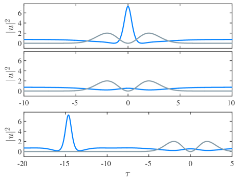
Figure 2: Temporal profiles of the intracavity field envelope $|u|^{2}$ (blue line) for the three fundamental CS states of the system. In this example, the effective potential, $V_{\rm eff}=(\phi^{\prime})^{2}$ (solid grey line) is not varying in the evolution variable (i.e., has constant $\tau_{0}$) in the three panels with parameters $\sigma_{\phi}=2$ and $h_{\phi}=4.6633$ (i.e., a maximum height of the tweezer of 2). The top panel is an example of a trapped CS (tweezed CS). The middle panel is an example of no soliton solution (no-CS). The bottom panel is an example of a CS is located outside of the effective potential and a no-CS is found inside the effective potential (called non-tweezed CS).

Let us now use the NCVA equations of motion to describe the dynamics of CSs subject to the tweezing in Eq. (11) in order to assess its tweezability as a function of $\tau_{f}$ (how far we want to tweeze) and $\beta$ (how adiabatic is the tweezing).

4 Temporal Tweezing

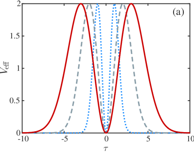
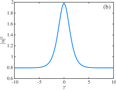
Figure 3: (a) Tweezers consisting of effective potentials of constant height with narrow, natural, and wide widths. The narrow tweezer (blue dotted line) is composed of phase modulation with $\sigma_{\phi}=1$ and $h_{\phi}=2.3316$. The natural width tweezer (grey dashed line) is composed of phase modulation with $\sigma_{\phi}=2$ and $h_{\phi}=4.6633$. The wide tweezer (red solid line) is composed of phase modulation with $\sigma_{\phi}=3$ and $h_{\phi}=6.9949$. The values of $h_{\phi}$ are chosen using Eq. (17) such that the height of the tweezer is always equal to 2. (b) The density of a cavity soliton in the absence of a tweezer, which has a natural width of $\approx 1.5$.

We explore the existence and dynamical properties for a tweezed cavity soliton in the effective potential described by $V_{\rm eff}=(\phi^{\prime})^{2}$ (also referred to as the “tweezer”). Before embarking on the dynamical tweezability of CSs, we must know what are the different possible scenarios. In particular, for a static tweezer (i.e., constant $\tau_{0}$) there are three fundamental states corresponding to the following qualitatively different scenarios: (a) a CS inside the tweezer, (b) no-CS in the system, and (c) a CS outside of the tweezer. These three scenarios are depicted in Fig. 2 for $\sigma_{\phi}=2$ and $h_{\phi}=4.6633$ (corresponds to a tweezer of maximum height 2; see Fig. 3). If we now consider a varying tweezer [i.e., $\tau_{0}$ given by Eq. (11)], for constant values of $\sigma_{\phi}$ and $h_{\phi}$, there will be critical values of $\beta$ and $\tau_{f}$ in Eq. (11) corresponding to thresholds between these fundamental states. We now proceed to provide a characterization of the existence of the three states for the full LL Eq. (6) and compare to the results of the NCVA with respect to the parameters $\beta$ and $\tau_{f}$. In what follows, we study different tweezing possibilities over the parameter space spanned by $\tau_{f}$, the final temporal displacement, and $\beta$, the degree of adiabaticity for the speed of the tweezer. A fully tweezed CS will correspond to a CS that stays inside the effective potential as the tweezer is displaced.

Rather than analyzing the individual evolution of temporal profiles, we can express the various states by the power contained inside and outside of the effective potential. For the full LL model, the CS temporal density $\rho=|u|^{2}$ and the no-CS temporal density $\rho_{0}=|u_{\rm{no\text{-}CS}}|^{2}$ are expressed by the power inside the tweezer $P_{\rm I}(z)$ and outside the tweezer $P_{\rm O}(z)$ which are given respectively by

$$P_{\rm I}(z)=\int_{\mathcal{D}}(\rho-\rho_{0})d\tau,$$ (15a)

$$P_{\rm O}(z)=\int_{\bar{\mathcal{D}}}(\rho-\rho_{0})d\tau,$$ (15b)

where ${\mathcal{D}}=[-\sigma,\sigma]$ is the domain of the tweezer which is defined as a symmetric interval around $\tau_{0}$ containing the maxima of the effective trap and $\bar{\mathcal{D}}$ is the complement of ${\mathcal{D}}$. Note that we subtracted the no-CS power, $\rho_{0}$, in order to counter the effects of the pedestal (constant steady state background) and ensure the power for a CS is positive. We thus define the total power of the solution by

$$P_{\rm Tot}=\int_{-\infty}^{+\infty}(\rho-\rho_{0})d\tau=P_{\rm I}+P_{\rm O}.$$

For the NCVA, we use the variational parameters and construct the CS temporal density $\bar{\rho}=|\bar{u}|^{2}$ and extract the power inside the tweezer $P_{\rm I}(z)$ and outside the tweezer $P_{\rm O}(z)$ which are given, respectively, by

$$\bar{P}_{\rm I}(z)=\int_{\mathcal{D}}\bar{\rho}d\tau,$$

$$\bar{P}_{\rm O}(z)=\int_{\bar{\mathcal{D}}}\bar{\rho}d\tau,$$

where ${\mathcal{D}}$ and $\bar{{\mathcal{D}}}$ are the same intervals described above and recall that in the construction of the NCVA ansatz we already subtracted out the effects of the background pedestal. The relative power change during the tweezing, namely between $z=0$ and $z=z_{f}$, is then defined by

$$Q_{\rm I}=\frac{P_{\rm I}(0)-P_{\rm I}(z_{f})}{P_{\rm Tot}},$$ (16a)

$$Q_{\rm O}=\frac{P_{\rm O}(0)-P_{\rm O}(z_{f})}{P_{\rm Tot}},$$ (16b)

for, respectively, the inside and outside of the tweezer. The same definition is used for the relative power changes ensuing from the NCVA approach.

By considering $Q_{\rm I}$ and $Q_{\rm O}$, we can effectively find the thresholds between the various states in the relevant $(\beta,\tau_{f})$ parameter space. For example, if we begin with a steady state CS inside the tweezer at $\tau_{0}=0$ and move with a given $\beta$ and $\tau_{f}$, then a successfully tweezed CS will result on approximately the same powers at $z=0$ as $z=z_{f}$ such that $P_{\rm I}(0)\approx P_{\rm I}(z_{f})$ as well as $P_{\rm O}(0)\approx P_{\rm O}(z_{f})$, and thus resulting in power ratios $Q_{\rm I}\approx 0\approx Q_{\rm O}$. On the other hand, if the CS dissipates away we are left solely with no-CS inside the tweezer and, thus, then $Q_{\rm I}\approx 1$ and $Q_{\rm O}\approx 0$. Finally, if at the end of the tweezing, a non-tweezed CS state ensues outside of the tweezer and a no-CS inside the tweezer, the resulting power changes will yield $Q_{\rm I}\approx 1$ and $Q_{\rm O}\approx-1$.

For our analysis, we select three different tweezers with a fixed height and a narrow, natural, and wide width corresponding to $\sigma_{\phi}=1$, 2, and 3, respectively. The relevant scales are determined in comparison to the intrinsic width of the CS in the absence of a tweezer. In order to maintain a constant maximum height of the effective potential $V_{\rm eff}$ equal to 2 [such that we have a deep enough trapping to contain the CS and that it matches the height of a natural CS in the absence of a tweezer; see Fig. 3(b)], we solve for the height of Eq. (8)

$$h_{\phi}=\frac{\sqrt{2}\sigma_{\phi}^{2}}{\max[\tau\exp(-\tau^{2}/2\sigma_{\phi}^{2})]}.$$ (17)

Figure 3(a) depicts the effective potentials $V_{\rm eff}=(\phi^{\prime})^{2}$ used for the three tweezer cases we are interested in studying: (i) tweezers with a “natural” width of $\sigma_{\phi}=2$ (grey dashed line); see Sec. 4.1, (ii) “narrow” tweezers with $\sigma_{\phi}=1$ (blue dotted line); see Appendix A.1, and (iii) “wide” tweezers with $\sigma_{\phi}=3$ (red solid line); see Appendix A.2. For comparison, Fig. 3(b) shows the density of a CS in the absence of a tweezer, which has a natural width $\sigma\approx 1.5$. For all example cases to follow, we keep the holding beam constant at $u_{\rm in}=2$.

4.1 Tweezer with Natural Width

In this section we report on the case study of a tweezer with a “natural” width that is close to the intrinsic width of the CS in the absence of the tweezer. In particular, we choose a tweezer width with $\sigma_{\phi}=2$ and height $h_{\phi}=4.6633$ (so that the maximum height of the tweezer is 2). The cases of a narrow and a wide tweezer are presented in the Appendix A. For the full LL Eq. (6), the steady state CS is found centered at $\tau_{0}=0$ using a Newton-Krylov solver supplemented with the power-balance constraint Eq. (7) which selects a detuning parameter value of $\Delta=2.8357$. The same $\Delta$, $\sigma_{\phi}$, and $h_{\phi}$ are used in the NCVA with a Newton-Krylov solver to find the initial variational parameters for the system. The parameter space for $\beta$ and $\tau_{f}$ is discretized into 41 steps between 0.1 and 20 in both directions, giving 1681 combinations for $\tau_{0}(z)$ as per Eq. (11). The full LL Eq. (6) is solved using a standard second order finite difference scheme in space and a standard fourth order Runge-Kutta method in time. It is relevant to note that the integration of the NCVA system of ODEs required the use of a stiff ODE solver and thus we used Matlab’s ode15s. Both the full LL PDE and the NCVA ODEs are evolved until $z_{f}=4z^{*}$, with $z^{*}=2.5$ (see Fig. 1) which ensures that the tweezed and/or non-tweezed CS had enough time to converge towards their steady state.

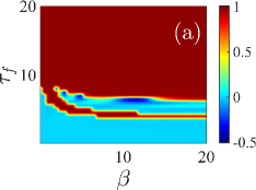
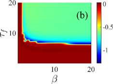
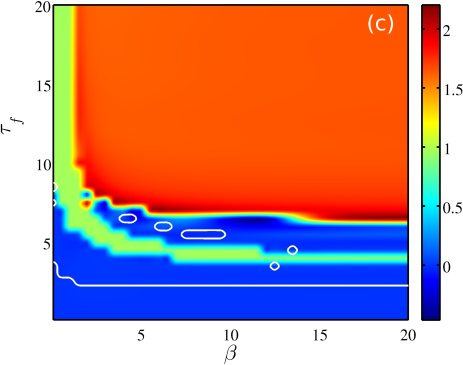
Figure 4: Power ratios (a) inside, $Q_{\rm I}$ and (b) outside, $Q_{\rm O}$, for a natural width tweezer with $\sigma_{\phi}=2$ and $h_{\phi}=4.6633$ (corresponding to a tweezer height of 2; see Fig. 3) as a function of the adiabaticity parameter $\beta$ and the tweezing distance $\tau_{f}$. The detuning for the system is $\Delta=2.8357$ and each combination of parameters is evolved for $z_{f}=4z^{*}$ with $z^{*}=2.5$. (a) For the power ratio inside the tweezer, $Q_{\rm I}$, the blue areas ($Q_{\rm I}\approx 0$) correspond to the power concentrated inside of the tweezer located at $z_{f}$ (namely, successful tweezing) while red areas ($Q_{\rm I}\approx 1$) correspond to no power concentrated inside the tweezer. (b) For the power ratio outside the tweezer, $Q_{\rm O}$, regions where $Q_{\rm O}<0$ correspond to cases where the zone outside of the tweezer gained power during tweezing implying that the tweezer could not hold the CS and it was left behind. Panel (c) depicts the difference between the inside and outside power ratios $\Delta Q=Q_{\rm I}-Q_{\rm O}$. A value of $\Delta Q\gtrsim 1.5$, orange region, corresponds to a non-tweezed CS (i.e., CS was left behind by tweezer), a value of $\Delta Q\approx 1$ (green region) corresponds to a no-CS (the CS got dissipated out during the tweezing process), and a value of $\Delta Q\approx 0$ (blue region) corresponds to a successfully tweezed CS. The middle blue inlet corresponds to a release and recapture scenario; see text. The white line corresponds to the contour at 0.5 for the NCVA threshold between tweezed and non-tweezed states.

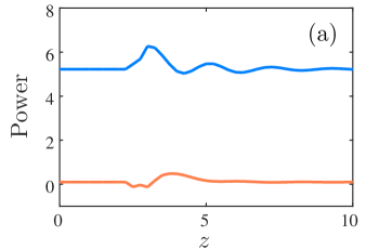
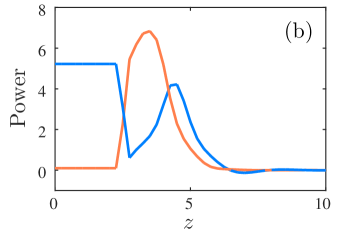
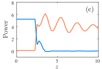
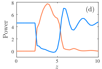
Figure 5: Evolution of the power inside the tweezer $P_{\rm I}$ (orange line) and the power outside the tweezer $P_{\rm O}$ (blue line) for the different tweezing scenarios. The system parameters correspond to: (a) $\tau_{f}=2$ and $\beta=10$, (b) $\tau_{f}=4.5$ and $\beta=10$, (c) $\tau_{f}=12$ and $\beta=10$, and (d) $\tau_{f}=5.5$ and $\beta=8$. Panel (a) depicts a sample case with no change in power inside or outside the tweezer which describes a successfully tweezed CS. See the actual dynamics of this case in Fig. 6 corresponding to the bottom blue region in Fig. 4. Panel (b) depicts a sample case where both powers inside and outside tend to vanish corresponding to a no-CS where the CS gets dissipated during the tweezing attempt. See the actual dynamics of this case in Fig. 7 corresponding to the green region in Fig. 4). Panel (c) depicts a sample case where the power inside and outside of the tweezer exchange and thus signaling a the tweezing was not sufficiently slow and a the CS drops of the tweezer and remains there. See the actual dynamics of this case in Fig. 8 corresponding to the see orange region in Fig. 4. Finally, panel (d) depicts a sample case of a fortuitous tweezing where a CS is initially ($z\approx 2$) dropped by the tweezer, but later ($z\gtrsim 6$) it is recaptured by the tweezer. See the actual dynamics of this case in Fig. 9 corresponding to the middle blue region in Fig. 4.

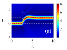
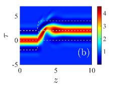
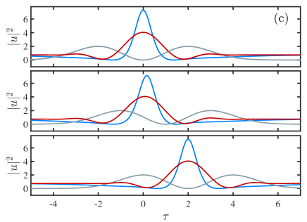
Figure 6: Evolution of the field for the example of the successful tweezing case depicted in Fig. 5(a) and corresponding to the bottom blue region in Fig. 4. Panels (a) and (b) depict, respectively, the evolution of the power of the field $|u(z,\tau)|^{2}$ from the full LL model and the reconstructed one from the NCVA approach. The dashed white curves depict the trajectory of the center of the tweezer $\tau_{0}(z)$ and one width away on each side ($\tau_{0}(z)\pm\sigma_{\phi})$. Panel (c) depicts snapshots of the power of the field at three different instances of the tweezing attempt corresponding to: initial configuration (top), configuration half way ($z=z^{*}$) through the tweezing attempt (middle), and final configuration ($z=z_{f}$). In each case the effective tweezing potential is depicted by the gray curve and the fields for the full LL and the NCVA approach are depicted, respectively, by the blue and red curves. The parameters for this case correspond to $\tau_{f}=2$ and $\beta=10$. In this case, both the LL model and its NCVA approach display a successful tweezing of the CS from $\tau=0$ to $\tau=\tau_{f}$.

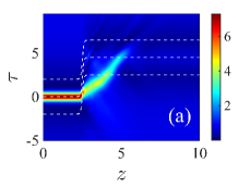
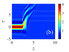
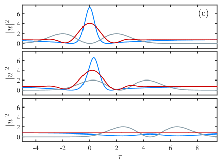
Figure 7: Evolution of the field for the example of the no-CS tweezing case depicted in Fig. 5(b) and corresponding to the green region in Fig. 4. Same layout as in Fig. 6. The parameters for this case correspond to $\tau_{f}=4.5$ and $\beta=10$. In this case, both the LL model and its NCVA approach display a no-CS scenario where the CS dissipated away during the tweezing attempt.

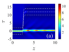
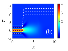
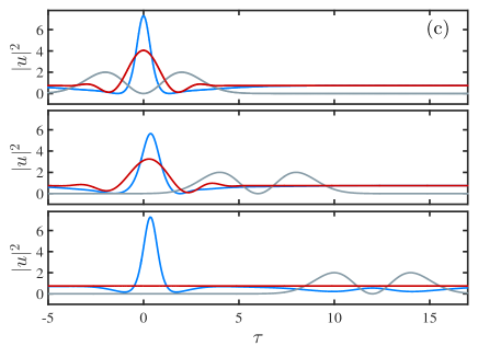
Figure 8: Evolution of the field for the example of the non-tweezed case depicted in Fig. 5(c) and corresponding to the orange region in Fig. 4. Same layout as in Fig. 6. The parameters for this case correspond to $\tau_{f}=12$ and $\beta=10$. In this case, the LL model displays a non-tweezed scenario where the CS is left behind by the tweezer. In contrast, the NCVA approach is not capable of directly reproducing non-tweezed scenarios and actually displays a no-CS one.

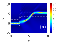
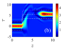
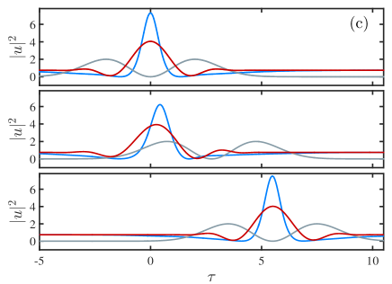
Figure 9: Evolution of the field for the example of the CS recaptured case depicted in Fig. 5(d) and corresponding to the middle blue region in Fig. 4. Same layout as in Fig. 6. The parameters for this case correspond to $\tau_{f}=5.5$ and $\beta=8$. In this case, both the LL model and its NCVA approach display a recapturing scenario where the CS is initially dropped by the tweezer but later recaptured.

We will now focus on following the power ratios $Q_{\rm I}$ and $Q_{\rm O}$ from Eqs. (16) for the different parameter combinations. Specifically, Fig. 4 depicts these power ratios as a function of the adiabaticity parameter $\beta$ and the tweezing distance $\tau_{f}$. Panels (a) and (b) depict, respectively, the power ratios inside and outside the tweezer for the case of a tweezer with natural width. In order to identify the different dynamical regions, both $Q_{\rm I}$ and $Q_{\rm O}$ need to be analyzed simultaneously. For example $Q_{\rm I}\approx 0$ is either a no-CS for $Q_{\rm O}\approx 0$ or a non-tweezed CS for $Q_{\rm O}\approx 1$. Therefore, for a more compact interpretation of the results, we use the difference in power ratios, $\Delta Q=Q_{\rm I}-Q_{\rm O}$, such that its values represent the following tweezing scenarios:

• $\circ~{}~{}\Delta Q\approx 0$: successful tweezing,

• $\circ~{}~{}\Delta Q\approx 1$: no-CS (i.e., the CS got dissipated out during the tweezing process),

• $\circ~{}~{}\Delta Q\gtrsim 1.5$: non-tweezed CS (the CS was left behind by the tweezer).

For instance, Fig. 4(c) depicts $\Delta Q$ as a function of $\beta$ and $\tau_{f}$ where the above three different tweezing regions are clearly defined: (i) successful tweezing ($\Delta Q\approx 0$) in blue, (ii) no-CS ($\Delta Q\approx 1$) in green, and (iii) non-tweezed CS ($\Delta Q\gtrsim 1.5$) in orange. The behavior of $\Delta Q$ in Fig. 4(c) confirms the existence of three fundamental states: a tweezed CS for all $\beta$ when $\tau_{f}<4$ (blue region), no-CS (green region), and a non-tweezed CS (orange/red regions).

Interestingly, there is a blue “inlet” region between the green and the orange regions. After further inspection, it turns out that this effectively successful tweezing region is a rather fortuitous one (or at least less expected). This region correspond to the peculiar case where the tweezer moves fast enough so that the CS is left behind but, at the same time, the tweezer moves slow enough so that it momentarily carries the CS and thus leaving it with some momentum such as, when it is released, it acquires a non-zero velocity towards the direction of the tweezer. As a result, the CS initially leaves the tweezer but continues to advance with a velocity slower than that of the tweezer at the time of the release. Then, as the tweezer arrives at its destination $z_{f}$ and slows down, the CS “catches up” with the tweezer before $\tau_{f}$ and gets recaptured by the tweezer. Thus this middle inlet of successful tweezing correspond to a case of release and recapture rather than a controllable tweezing scenario. With this is mind, we can conclude that, with the current parameter values that we used, a combination of $0<\beta<20$ with $\tau_{f}\lesssim 4$ ensures a proper and successful tweezing of the CS.

On the other hand, we also followed the tweezing scenarios under the NCVA approximation. For the NCVA system, there are only two fundamental scenarios a tweezed CS and a no-CS solution. However, our study suggests that there is no NCVA solution in which the tweezer leaves behind a CS. Therefore, in as far as the NCVA description is concerned, it is not necessary to use $Q_{\rm O}$ since both NCVA outcomes result in $Q_{\rm O}\approx 0$. Figure 4(c) overlays on top of the full LL PDE results, a contour corresponding to the NCVA results for $\Delta Q=0.5$ (see white line). This allows us to compare the tweezing threshold separating a tweezed CS and no-CS solution for the full LL model and its NCVA reduction. As we may conclude, the NCVA is able to correctly capture the qualitative aspects of the tweezing of the original full LL system and, to some extent, it also provides approximate quantitative information. For instance, as we discussed above, successful tweezing in the full LL system happens for $\tau_{f}\lesssim 4$ and the NCVA predicts successful tweezing for $\tau_{f}\lesssim 3$. Furthermore, it is interesting to note that in the middle (blue) inlet region corresponding to the release and recapture scenarios for the full LL equation, the NCVA predicts small islands of successful tweezing. Thus, in some sense, the NCVA is able to compromise and give a positive tweezing outcome in this release and recapture region.

In order to better understand the results presented above, we now describe representative examples for the four different tweezing scenarios presented above. Namely, (i) successful tweezing, (ii) no-CS, (iii) non-tweezed, and (iv) CS recapture. Figure 5 depicts the evolution of the power inside $P_{\rm I}(z)$ and the power outside $P_{\rm O}(z)$ during the tweezing period $0\leq z\leq z_{f}$ for typical examples of the four different tweezing scenarios. Finally, for completeness, Figs. 6–9 depict the actual evolution of the field for these four representative cases. Each of these figures depicts the full evolution of the power of the field $|u(z,\tau)|^{2}$ during the tweezing attempt where the respective panels (a) depict the the field from the full LL model and the respective panels (b) depict the reconstructed field from the NCVA approach. The respective panels (c) depict the field at three different stages during the tweezing attempt. Namely, top subpanel: initial configuration $z=0$, middle subpanel: half way through the tweezing $z=z^{*}$, and bottom subpanel: end of the tweezing procedure $z=z_{f}$ (see Fig. 1).

An example of a successful tweezing scenario is depicted in Fig. 6 and corresponds to a case in the bottom blue region in Fig. 4. Here, both the full LL model and the NCVA approach display a successful tweezing of the CS from $z=0$ to $z=z_{f}$. An example of a no-CS case is depicted in Fig. 7 and corresponds to a case in the green region in Fig. 4. Here, both the full LL model and the NCVA approach display a no-CS tweezing where the CS is dissipated away during tweezing. Figure 8 depicts a non-tweezed scenario corresponding to a case in the orange region in Fig. 4. Here, the LL model displays a non-tweezed scenario where the CS is left behind by the tweezer while the NCVA approach, not capable of directly reproducing non-tweezed scenarios, displays a no-CS scenario. Finally, an example of a CS recapture scenario is depicted in Fig. 9 and corresponds to a case in middle blue region in Fig. 4. Here, both the full LL model and the NCVA approach display a CS that is initially dropped by the tweezer but later recaptured, upon propagation of the wave towards the final position of the tweezer.

For completeness, along with the examples described above, Appendix A presents similar scenarios for the case of a tweezer that is narrower than the CS (see Appendix A.1) and a tweezer that is wider than the CS (see Appendix A.2).

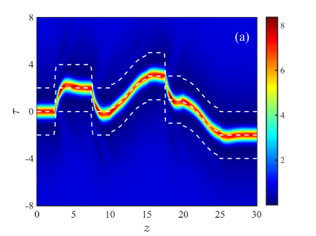
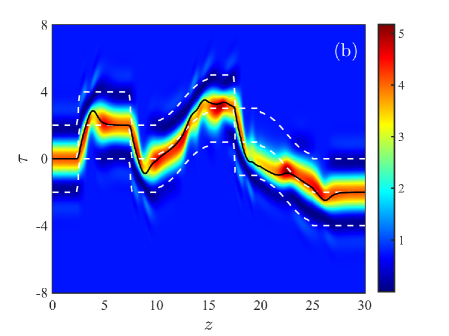
Figure 10: Dynamic evolution of a CS using a zigzagging tweezer with different degrees of adiabaticity by varying $\tau_{f}$ and $\beta$ (see text for details). Same meaning as in panels (a) and (b) of Fig. 6, namely, panel (a) corresponds to the full LL model while panel (b) corresponds to the NCVA approach. Both the LL model (a) and NCVA (b) CS solution continues to follow the prescribed trajectory despite the tweezer being moved back-and-forth at various speeds. In panel (b) the black line is the NCVA variational parameter $\xi$. This sample serves to illustrate how a CS can be robustly manipulated given various degrees of adiabaticity.

4.2 Demonstration of a Non-trivial Temporal Tweezing

Now that we have studied the parameter regions that give rise to the different tweezing scenarios, let us demonstrate the robustness of the CS manipulation when using tweezer parameters $\tau_{f}$ and $\beta$ inside the tweezability region. In particular, Fig. 10 depicts a more general tweezing scenario where, instead of a single value for the parameters $\tau_{f}$ and $\beta$, we change the parameters at set increments in $z$. Specifically, we choose a nontrivial back-and-forth tweezing “trajectory” with a zigzagging motion separated in five subintervals with different degrees of adiabaticity as follows. For $0\leq z\leq 5$, $\tau(0)=0$, $\tau(5)=2$, and $\beta=10$, then for $5<z\leq 10$, $\tau(5)=2$, $\tau(10)=0$, and $\beta=10$, then for $10<z\leq 15$, $\tau(10)=0$, $\tau(15)=3$, and $\beta=0.5$, then for $15<z\leq 20$, $\tau(15)=3$, $\tau(20)=1$, and $\beta=20$, then for $20<z\leq 25$, $\tau(20)=1$, $\tau(25)=-2$, and $\beta=0.5$. As Fig. 10 shows, the CS is successfully tweezed along this complicated zigzagging orbit (see middle white dashed curve), thus showcasing the robustness of the tweezing mechanism for the full LL dynamics [shown in panel (a)]. Furthermore, as panel (b) shows, the NCVA reduction of the LL system is also able to predict and reproduce the successful tweezing of the CS along the zigzagging orbit. In the case of the NCVA approach in panel (b), the additional black line depicts the ansatz parameter $\xi$ which follows the center position of the tweezer $\tau_{0}$. This example suggests that, through an appropriate manipulation of the phase-modulation of the holding beam, it is possible to trap and move the CS at will based on the proposed tweezing mechanism and for a (revealed herein) wide interval of the associated dynamical parameters.

5 Conclusions and Future Challenges

In Ref. [4] the authors showed experimentally that a cavity soliton (CS) stored in a passive loop of optical fiber could be temporally tweezed by manipulating the phase-modulation of the holding beam. Motivated by this experimental work, we studied herein the possibility of tweezing more generally CSs using various profiles of the holding beam and in particular varying the degree of adiabaticity used in the tweezing “trajectory”’. We modeled the system using a variant of the complex Ginzburg-Landau (cGL) equation in the form of the Lugiato-Lefever (LL) partial differential equation with additional terms accounting for the incorporation of the tweezer from the phase-modulation of the holding beam.

In our study, we assume a Gaussian phase-modulation that gives rise to an effective tweezer potential, proportional to the derivative of the phase-modulation profile, that takes the shape of a localized two-hump trapping profile. For three different widths of the tweezer, when compared to the intrinsic (natural) width of the CS in the absence of phase modulation, corresponding to (i) a tweezer width close to the CS width, (ii) a tweezer narrower than the CS width, and (iii) a tweezer slightly wider than the CS width (with the latter two being in Appendix A), we study the effects of the temporal tweezing ‘distance’ ($\tau_{f}$) and the maximum tweezing motion speed (controlled by the parameter $\beta$) on the success (or not) of the resulting tweezing scenario of the CS. We find that, depending on the tweezer width and the parameters $\tau_{f}$ and $\beta$, four different outcomes are possible as the degree of adiabaticity is varied. These four cases correspond to (ordered from the most adiabatic to the least adiabatic cases): (a) For sufficiently slow tweezing motion, the tweezer is generically capable of transporting the CS to any desired location. (b) As the tweezer’s speed is increased we encounter cases where the tweezer is not able to hold the CS and thus the latter falls behind. However, if the tweezer’s speed is relatively small such that the CS is initially momentarily carried by the tweezer, as it is dropped, it carries a finite velocity in the direction of the tweezer. Thus, when the tweezer slows down and eventually stops at the final location, the CS “catches up” and gets recaptured. This corresponds to a release and recapture scenario. (c) Increasing further the tweezer’s speed results on a non-trivial interaction of the CS and the tweezer where the CS is completely absorbed and disappears. (d) Finally, for relatively large tweezer’s speeds the CS slides out of the tweezing potential and is left behind to exist in the bulk of the medium while the tweezer moves away without carrying along the CS. Furthermore, a comparison between the tweezability regions in parameter space for the three tweezer widths that were explored suggests that a slightly wider tweezer potential than the natural width of the CS is the most efficient scenario in order to produce successful tweezing for a wider range of control parameters.

As part of our theoretical study, we develop a Lagrangian formalism for the modified LL equation that intrinsically includes gain and loss terms. To tackle this out-of-equilibrium, non-Hamiltonian, system we use the recently developed non-conservative variational approximation (NCVA) of Ref. [24], based on the earlier formulation of Refs. [42, 43]. We use the NCVA approach with an appropriately crafted CS ansatz to reduce the original LL dynamics (a partial differential equation) to a set of coupled ordinary differential equations on the ansatz parameters (height, position, width, phase, velocity, and chirp). We show how the NCVA reduction approach is able to qualitatively, and to some extent quantitatively, describe the different tweezing scenarios [with the exception of case (d) above]. In particular, we notice that the NCVA is capable of predicting the threshold in the tweezer parameter space for tweezed CSs, case (a), and dissipated CS states, case (b), although it is not adequate for fully capturing more complex dynamics (especially so for tweezers with large displacements and speeds).

Our analysis of temporal tweezing offers insights into the design of localized tweezers used in optical information processing, which requires the ability to trap ultrashort pulses of light and dynamically move them around in time, with respect to, and independently of other pulses of light. In particular, from our study of the LL equation and the NCVA approach, we have developed a process to identify regions of tweezability which can aid toward the experimental design and identification of regimes of reliability of temporal tweezing used for information processing.

A possible extension of this work pertains the case of a periodic modulation of the holding beam that induces a periodic effective tweezer potential. It would be interesting to study in detail the possible manipulation of the CSs using such periodic modulation as it was studied in Refs. [20, 21] for the (otherwise conservative) nonlinear Schrödinger case. Another avenue of potential interest would be the study of tweezability of vortices in the presence of gain and loss similar to what has been reported in the conservative case of the nonlinear Schrödinger equation; see Refs. [47, 48] and references therein. In general, the extension of considerations presented herein for one spatial dimension to the context of higher-dimensional settings would be a particularly interesting direction for future work.

In reference to temporal tweezing, multiple CSs can be present simultaneously and independently at arbitrary locations in a passive loop of optical fiber. Therefore, a relevant extension would be to add interactions of multiple CSs in the system. Investigating the dynamics, interactions, and tweezability of the CS by allowing for long-range soliton interactions is necessary to understand an effective treatment of a CS, each of which constitute an ideal bit in optical information processing. It is relevant to mention in that regard that the recent review of Ref. [49] has summarized the extensive control that this framework enables both in the way of phase, as well as of intensity of the inhomogeneous driving field. Additionally, recent experiments of pulsed driving are also discussed therein towards the direction of producing flexible and efficient optical frequency combs. Another possible extension of the temporal tweezing study is to analyze the linearization spectrum of the system and identify the stability/instability transitions between the different states we identified. In this same vein, the identification of the spectrum can be used with the Galerkin approach capable of capturing bifurcations induced by changing the speed of the tweezer. Indeed, it would be interesting to identify the co-traveling states in the case of a traveling tweezer and to identify whether the transition, e.g., from tweezing to disappearance of the pulse can be identified with a bifurcation phenomenon. Such directions are currently in progress and will be reported in future publications.

Appendix A Additional Temporal Tweezers

In this Appendix, we present additional tweezing results to complement the results presented in Sec. 4. In particular, in Sec. 4.1 we studied the dynamics when using a tweezer with a width that is comparable to the width of the CS, what we called a “natural” width. Here we present in Secs. A.1 and A.2 similar results but for a tweezer that is, respectively, narrower and wider than the CS.

A.1 Narrow Tweezers

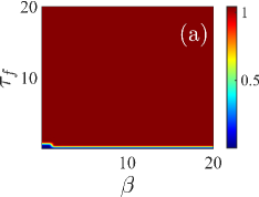
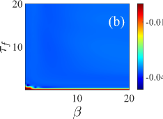
Figure 11: Same meaning and layout as in Fig. 4 for a narrow tweezer with $\sigma_{\phi}=1$ and $h_{\phi}=2.3316$ (leading to a tweezer potential of height 2). In this case the detuning for the system is $\Delta=4.1692$.

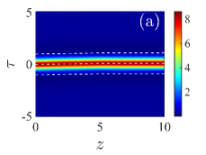
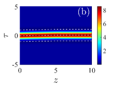
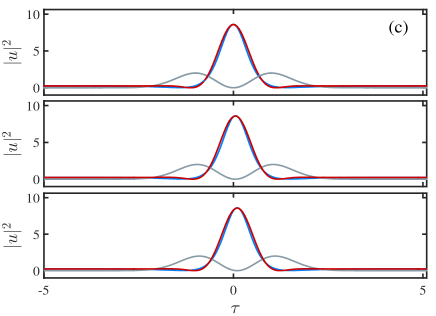
Figure 12: Same meaning and layout as in Fig. 6 for the narrow tweezer with $\sigma_{\phi}=1$ and $h_{\phi}=2.3316$. This case with $\tau_{f}=0.1$ and $\beta=0.1$ corresponds to a successful tweezing of the CS. Note that this rather small value of $\tau_{f}$ induces a very small (temporal) displacement of the tweezed CS. The smallness of this value for $\tau_{f}$ stems from the narrow region of tweezability for the narrow width tweezer as depicted in Fig. 11.

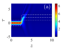
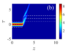
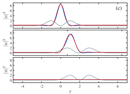
Figure 13: Dynamic evolution as in Fig. 12 but for $\tau_{f}=2$ and $\beta=10$. Same layout as in Fig. 12. In this sample, both the LL model solution and NCVA are a no-CS.

The first supplemental example that we show corresponds to a tweezer with a “narrow” width $\sigma_{\phi}=1$. This width is to be compared with the intrinsic (natural) width of the CS in the absence of the holding beam. For this case, as we have done throughout this work, we keep a height of the effective tweezer potential of 2 and thus $h_{\phi}=2.3316$ from Eq. (17). Also for this case, the power-balance constraint (7) selects a detuning parameter value of $\Delta=4.1692$. All the other parameters and the methodology are the same as the ones used for the natural width tweezer of Sec. 4. The main results for the narrow tweezer are depicted in Fig. 11 and should be contrasted with the results for the natural width tweezer depicted in Fig. 4. Comparing to the natural width tweezer case, the full LL model with a narrow tweezer has a much wider region of no-CSs (red region with $Q\approx 1$) and a much narrower region of successful CS tweezing (blue region with $Q\approx 0$). In tandem, the NCVA approach also displays a much narrower region of tweezability in this case which matches qualitatively and, to some extent, quantitatively the full LL model (with the notable exception of small isolated islands that lead to tweezing for the NCVA approach where the full LL model has no successful tweezing). Note that when compared to the natural width tweezer case, the narrower tweezer case does not seem to display non-tweezed CS nor recapture regions. In fact, for the narrow tweezer we only observe, for both the full LL model and its NCVA approach reduction, two scenarios corresponding to a successful tweezing as depicted in Fig. 12 and a no-CS case as depicted in Fig. 13. Apparently, the narrow tweezer is only capable of successfully tweezing the CS for extremely slow (adiabatic) tweezing trajectories —in this case the maximum (temporal) distance $\tau_{f}$ for successful tweezing is extremely small (smaller than one as evidenced in Fig. 11). The lesson learned from this section is that choosing carefully the width of the effective tweezer potential is essential to enhance the tweezability of the CSs. In particular, if the tweezer is narrower than the natural width of the CS in the absence of the tweezer, tweezing is severely compromised.

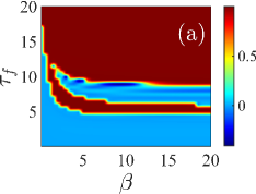
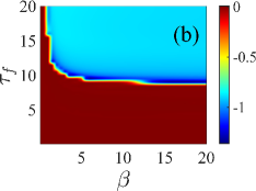
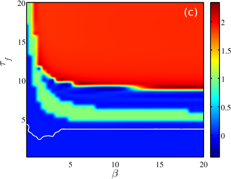
Figure 14: Same meaning and layout as in Fig. 11 but for a tweezer with a wide width of $\sigma_{\phi}=3$ and $h_{\phi}=6.9949$. The detuning for the system is $\Delta=3.0859$.

A.2 Wide Tweezers

The last supplemental example that we are interested in corresponds to a wide tweezer when compared to the natural width of the untrapped CS. In particular, we choose a tweezer width of $\sigma_{\phi}=3$ with $h_{\phi}=6.9949$ to keep, as before, the maximum height of the effective tweezer potential equal to 2. Also for this case, the power-balance constraint (7) selects a detuning parameter value of $\Delta=3.0859$. All the other parameters and the methodology are the same as the ones used for the natural width tweezer of Sec. 4. A quick comparison between the wide tweezer case depicted in Fig. 14 and the natural tweezer width case depicted in Fig. 4 reveals that these two cases are qualitatively similar for the full LL model. In fact, both cases present the four tweezing scenarios described in Sec. 4.1 and a similar placement of the regions ascribed to each of these scenarios. We have also checked the actual individual field density evolutions for these four scenarios and they are very similar to the ones presented in Figs. 6–9 and thus we opt not to show them here. It is interesting to mention that there is notable difference between the natural width tweezer and the wide tweezer width NCVA approach results in that the latter do not display the isolated islands of tweezability that are present for the natural tweezer width case (and also the narrow tweezer case).

A more careful comparison between the $\Delta Q$ results depicted in Figs. 4 and 14, reveals that the threshold for the existence of the tweezed CS with a wide tweezer is marginally larger than that found for a natural width tweezer. In fact, comparing the three sets of results presented in Sec. 4.1 (see Fig. 4), Sec. A.1 (see Fig. 11), and Sec. A.2 (see Fig. 14), suggests that a slightly wider tweezer potential than the natural width of the CS might be the most optimal scenario in order to produce successful tweezing for a wider range of parameters.

Appendix B NCVA System of Equations for Temporal Tweezing of Cavity Soliton

In this Appendix, we present the resulting modified Euler-Lagrange equations of motion from the LL Eq. (6) for temporal tweezing based on the NCVA where the over-dot denotes derivative with respect to $z$. For explicit integrals $I_{a}$, $I_{b}$, $I_{c}$, $I_{d}$, $I_{\sigma}$, and $I_{\xi}$ please see Appendix C.

$$\dot{a} =\frac{1}{4{a}{\sigma}^{3}{\sqrt{\pi}}\left({\sigma}^{2}+2\,{{\sigma_{\phi}}}^{2}\right)^{9/2}}\,\Bigg{[}-64\,{a}^{2}d\,{\sigma}^{9}\sqrt{\pi}B{{\sigma_{\phi}}}^{2}-192\,{a}^{2}d\,{\sigma}^{7}\sqrt{\pi}B{{\sigma_{\phi}}}^{4}-256\,{a}^{2}d\,{\sigma}^{5}\sqrt{\pi}B{{\sigma_{\phi}}}^{6}$$

$$-128\,{a}^{2}d\,{\sigma}^{3}\sqrt{\pi}B{{\sigma_{\phi}}}^{8}+48\,{\sigma}^{2}{I_{b}}\,B{{\sigma_{\phi}}}^{8}-16\,{I_{d}}\,B{\sigma}^{6}{{\sigma_{\phi}}}^{2}-48\,{I_{d}}\,B{\sigma}^{4}{{\sigma_{\phi}}}^{4}-64\,{I_{d}}\,B{\sigma}^{2}{{\sigma_{\phi}}}^{6}$$

$$-4\,{\sigma}^{11}\sqrt{\pi}{a}^{2}B+24\,{\sigma}^{8}{I_{b}}\,B{{\sigma_{\phi}}}^{2}+72\,{\sigma}^{6}{I_{b}}\,B{{\sigma_{\phi}}}^{4}+96\,{\sigma}^{4}{I_{b}}\,B{{\sigma_{\phi}}}^{6}+3\,{\sigma}^{10}{I_{b}}\,B$$

$$-2\,{I_{d}}\,B{\sigma}^{8}-32\,{I_{d}}\,B{{\sigma_{\phi}}}^{8}-224\,D{h_{\phi}}\,{{\sigma_{\phi}}}^{3}{\sigma}^{5}{a}^{2}\sqrt{2}\sqrt{\pi}{{\xi}}^{2}-80\,D{h_{\phi}}\,{\sigma_{\phi}}\,{\sigma}^{7}{a}^{2}\sqrt{2}\sqrt{\pi}{{\tau_{0}}}^{2}$$

$$+16\,{\sigma}^{5}\sqrt{\pi}{a}^{2}D\sqrt{2}{h_{\phi}}\,{{\tau_{0}}}^{4}{\sigma_{\phi}}-128\,D{h_{\phi}}\,{{\sigma_{\phi}}}^{5}{\sigma}^{3}{a}^{2}\sqrt{2}\sqrt{\pi}{{\tau_{0}}}^{2}-80\,D{h_{\phi}}\,{\sigma_{\phi}}\,{\sigma}^{7}{a}^{2}\sqrt{2}\sqrt{\pi}{{\xi}}^{2}$$

$$-224\,D{h_{\phi}}\,{{\sigma_{\phi}}}^{3}{\sigma}^{5}{a}^{2}\sqrt{2}\sqrt{\pi}{{\tau_{0}}}^{2}-128\,D{h_{\phi}}\,{{\sigma_{\phi}}}^{5}{\sigma}^{3}{a}^{2}\sqrt{2}\sqrt{\pi}{{\xi}}^{2}+16\,{\sigma}^{5}\sqrt{\pi}{a}^{2}D\sqrt{2}{h_{\phi}}\,{{\xi}}^{4}{\sigma_{\phi}}$$

$$+448\,D{h_{\phi}}\,{{\sigma_{\phi}}}^{3}{\sigma}^{5}{a}^{2}\sqrt{2}\sqrt{\pi}{\tau_{0}}\,{\xi}-8\,{a}^{2}d\,{\sigma}^{11}\sqrt{\pi}B-32\,{\sigma}^{9}\sqrt{\pi}{a}^{2}B{{\sigma_{\phi}}}^{2}-96\,{\sigma}^{7}\sqrt{\pi}{a}^{2}B{{\sigma_{\phi}}}^{4}$$

$$-128\,{\sigma}^{5}\sqrt{\pi}{a}^{2}B{{\sigma_{\phi}}}^{6}-64\,{\sigma}^{3}\sqrt{\pi}{a}^{2}B{{\sigma_{\phi}}}^{8}+240\,{{\sigma_{\phi}}}^{5}{\sigma}^{5}\sqrt{\pi}D\sqrt{2}{h_{\phi}}\,{a}^{2}+128\,{{\sigma_{\phi}}}^{7}{\sigma}^{3}\sqrt{\pi}D\sqrt{2}{h_{\phi}}\,{a}^{2}$$

$$+28\,{\sigma_{\phi}}\,{\sigma}^{9}\sqrt{\pi}D\sqrt{2}{h_{\phi}}\,{a}^{2}+144\,{{\sigma_{\phi}}}^{3}{\sigma}^{7}\sqrt{\pi}D\sqrt{2}{h_{\phi}}\,{a}^{2}+256\,D{h_{\phi}}\,{{\sigma_{\phi}}}^{5}{\sigma}^{3}{a}^{2}\sqrt{2}\sqrt{\pi}{\tau_{0}}\,{\xi}$$

$$-64\,{\sigma}^{5}\sqrt{\pi}{a}^{2}D\sqrt{2}{h_{\phi}}\,{{\xi}}^{3}{\tau_{0}}\,{\sigma_{\phi}}-64\,{\sigma}^{5}\sqrt{\pi}{a}^{2}D\sqrt{2}{h_{\phi}}\,{{\tau_{0}}}^{3}{\xi}\,{\sigma_{\phi}}+96\,{\sigma}^{5}\sqrt{\pi}{a}^{2}D\sqrt{2}{h_{\phi}}\,{{\tau_{0}}}^{2}{\sigma_{\phi}}\,{{\xi}}^{2}$$

$$+160\,D{h_{\phi}}\,{\sigma_{\phi}}\,{\sigma}^{7}{a}^{2}\sqrt{2}\sqrt{\pi}{\tau_{0}}\,{\xi}\Bigg{]},$$ (18)

$$\dot{b} =-\frac{1}{8{a}^{2}{\sqrt{\pi}}{\sigma}^{2}\left({\sigma}^{2}+{{\sigma_{\phi}}}^{2}\right)^{9/2}{{\sigma_{\phi}}}\left({\sigma}^{2}+2\,{{\sigma_{\phi}}}^{2}\right)^{9/2}}\,\Bigg{[}6\,{\sigma}^{18}C{{h_{\phi}}}^{2}{a}^{2}\sqrt{\pi}B-8\,{\sigma}^{17}A{\sigma_{\phi}}\,c\,{I_{c}}\,B$$

$$-96\,{\sigma}^{15}A{{\sigma_{\phi}}}^{3}c\,{I_{c}}\,B-496\,{\sigma}^{13}A{{\sigma_{\phi}}}^{5}c\,{I_{c}}\,B-1440\,{\sigma}^{11}A{{\sigma_{\phi}}}^{7}c\,{I_{c}}\,B-2568\,{\sigma}^{9}A{{\sigma_{\phi}}}^{9}c\,{I_{c}}\,B$$

$$-2880\,{\sigma}^{7}A{{\sigma_{\phi}}}^{11}c\,{I_{c}}\,B+1488\,{\sigma}^{5}{{\sigma_{\phi}}}^{13}{I_{a}}\,ABa+2568\,{{\sigma_{\phi}}}^{9}{a}^{2}\sqrt{\pi}AB{\sigma}^{8}+2880\,{{\sigma_{\phi}}}^{11}{a}^{2}\sqrt{\pi}AB{\sigma}^{6}$$

$$+1984\,{{\sigma_{\phi}}}^{13}{a}^{2}\sqrt{\pi}AB{\sigma}^{4}+768\,{{\sigma_{\phi}}}^{15}{a}^{2}\sqrt{\pi}AB{\sigma}^{2}+96\,AB{a}^{2}\sqrt{\pi}{{\sigma_{\phi}}}^{3}{\sigma}^{14}$$

$$+496\,AB{a}^{2}\sqrt{\pi}{{\sigma_{\phi}}}^{5}{\sigma}^{12}+1440\,AB{a}^{2}\sqrt{\pi}{{\sigma_{\phi}}}^{7}{\sigma}^{10}+8\,{a}^{2}\sqrt{\pi}A{\sigma_{\phi}}\,B{\sigma}^{16}-1984\,{\sigma}^{5}{{\sigma_{\phi}}}^{13}Ac\,{I_{c}}\,B$$

$$+576\,{\sigma}^{3}{{\sigma_{\phi}}}^{15}{I_{a}}\,ABa-768\,{\sigma}^{3}{{\sigma_{\phi}}}^{15}Ac\,{I_{c}}\,B+96\,{{\sigma_{\phi}}}^{17}{I_{a}}\,\sigma\,ABa$$

$$-128\,{{\sigma_{\phi}}}^{17}\sigma\,Ac\,{I_{c}}\,B+6\,{\sigma}^{17}{I_{a}}\,A{\sigma_{\phi}}\,Ba+72\,{\sigma}^{15}{I_{a}}\,A{{\sigma_{\phi}}}^{3}Ba+372\,{\sigma}^{13}{I_{a}}\,A{{\sigma_{\phi}}}^{5}Ba$$

$$+1080\,{\sigma}^{11}{I_{a}}\,A{{\sigma_{\phi}}}^{7}Ba+1926\,{\sigma}^{9}{I_{a}}\,A{{\sigma_{\phi}}}^{9}Ba+2160\,{\sigma}^{7}{I_{a}}\,A{{\sigma_{\phi}}}^{11}Ba$$

$$-1536\,AB\left(\left|{v}\right|\right)^{2}{a}^{2}{\sigma}^{4}\sqrt{\pi}{{\sigma_{\phi}}}^{15}-5\,{a}^{4}\sqrt{2}\sqrt{\pi}{\sigma}^{18}A{\sigma_{\phi}}\,B-80\,{a}^{4}\sqrt{2}\sqrt{\pi}{\sigma}^{2}A{{\sigma_{\phi}}}^{17}B$$

$$-60\,{a}^{4}\sqrt{2}\sqrt{\pi}{\sigma}^{16}A{{\sigma_{\phi}}}^{3}B-310\,{a}^{4}\sqrt{2}\sqrt{\pi}{\sigma}^{14}A{{\sigma_{\phi}}}^{5}B-900\,{a}^{4}\sqrt{2}\sqrt{\pi}{\sigma}^{12}A{{\sigma_{\phi}}}^{7}B$$

$$-1605\,{a}^{4}\sqrt{2}\sqrt{\pi}{\sigma}^{10}A{{\sigma_{\phi}}}^{9}B-1800\,{a}^{4}\sqrt{2}\sqrt{\pi}{\sigma}^{8}A{{\sigma_{\phi}}}^{11}B-1240\,{a}^{4}\sqrt{2}\sqrt{\pi}{\sigma}^{6}A{{\sigma_{\phi}}}^{13}B$$

$$-480\,{a}^{4}\sqrt{2}\sqrt{\pi}{\sigma}^{4}A{{\sigma_{\phi}}}^{15}B-128\,{{\sigma_{\phi}}}^{17}{a}^{2}{c}^{2}{\sigma}^{2}\sqrt{\pi}AB-768\,{\sigma}^{4}{{\sigma_{\phi}}}^{15}{a}^{2}{c}^{2}\sqrt{\pi}AB$$

$$+384\,BC{{h_{\phi}}}^{2}{a}^{2}{\sigma}^{8}\sqrt{\pi}{{\sigma_{\phi}}}^{10}+96\,BC{{h_{\phi}}}^{2}{a}^{2}{\sigma}^{6}\sqrt{\pi}{{\sigma_{\phi}}}^{12}+60\,{\sigma}^{16}C{{h_{\phi}}}^{2}{a}^{2}\sqrt{\pi}B{{\sigma_{\phi}}}^{2}$$

$$+246\,{\sigma}^{14}C{{h_{\phi}}}^{2}{a}^{2}\sqrt{\pi}B{{\sigma_{\phi}}}^{4}+528\,BC{{h_{\phi}}}^{2}{a}^{2}{\sigma}^{12}\sqrt{\pi}{{\sigma_{\phi}}}^{6}-4\,{\sigma}^{16}C{{h_{\phi}}}^{2}{a}^{2}\sqrt{\pi}B{{\tau_{0}}}^{2}$$

$$-4\,{\sigma}^{16}C{{h_{\phi}}}^{2}{a}^{2}\sqrt{\pi}B{{\xi}}^{2}+624\,BC{{h_{\phi}}}^{2}{a}^{2}{\sigma}^{10}\sqrt{\pi}{{\sigma_{\phi}}}^{8}-384\,{\sigma}^{10}C{{h_{\phi}}}^{2}{{\sigma_{\phi}}}^{4}{a}^{2}\sqrt{\pi}B{{\tau_{0}}}^{2}{{\xi}}^{2}$$

$$-1152\,{\sigma}^{8}C{{h_{\phi}}}^{2}{{\sigma_{\phi}}}^{6}{a}^{2}\sqrt{\pi}B{{\tau_{0}}}^{2}{{\xi}}^{2}-1536\,{\sigma}^{6}C{{h_{\phi}}}^{2}{{\sigma_{\phi}}}^{8}{a}^{2}\sqrt{\pi}B{{\tau_{0}}}^{2}{{\xi}}^{2}-768\,{\sigma}^{4}C{{h_{\phi}}}^{2}{{\sigma_{\phi}}}^{10}{a}^{2}\sqrt{\pi}B{{\tau_{0}}}^{2}{{\xi}}^{2}$$

$$+32\,{\sigma}^{12}C{{h_{\phi}}}^{2}{{\sigma_{\phi}}}^{2}{a}^{2}\sqrt{\pi}B{{\tau_{0}}}^{3}{\xi}+256\,{\sigma}^{10}C{{h_{\phi}}}^{2}{{\sigma_{\phi}}}^{4}{a}^{2}\sqrt{\pi}B{{\tau_{0}}}^{3}{\xi}+1632\,BC{{h_{\phi}}}^{2}{{\sigma_{\phi}}}^{8}{\sigma}^{8}{a}^{2}\sqrt{\pi}{{\tau_{0}}}^{2}$$

$$+1728\,BC{{h_{\phi}}}^{2}{{\sigma_{\phi}}}^{10}{\sigma}^{6}{a}^{2}\sqrt{\pi}{{\tau_{0}}}^{2}+832\,BC{{h_{\phi}}}^{2}{{\sigma_{\phi}}}^{12}{\sigma}^{4}{a}^{2}\sqrt{\pi}{{\tau_{0}}}^{2}+128\,BC{{h_{\phi}}}^{2}{{\sigma_{\phi}}}^{14}{\sigma}^{2}{a}^{2}\sqrt{\pi}{{\tau_{0}}}^{2}$$

$$-8\,BC{{h_{\phi}}}^{2}{{\sigma_{\phi}}}^{2}{\sigma}^{14}{a}^{2}\sqrt{\pi}{{\xi}}^{2}+132\,BC{{h_{\phi}}}^{2}{{\sigma_{\phi}}}^{4}{\sigma}^{12}{a}^{2}\sqrt{\pi}{{\xi}}^{2}+832\,C{{h_{\phi}}}^{2}{{\sigma_{\phi}}}^{12}{a}^{2}\sqrt{\pi}{\sigma}^{4}B{{\xi}}^{2}$$

$$+128\,C{{h_{\phi}}}^{2}{{\sigma_{\phi}}}^{14}{a}^{2}\sqrt{\pi}{\sigma}^{2}B{{\xi}}^{2}+8\,{\sigma}^{16}C{{h_{\phi}}}^{2}{a}^{2}\sqrt{\pi}B{\tau_{0}}\,{\xi}+744\,C{{h_{\phi}}}^{2}{{\sigma_{\phi}}}^{6}{a}^{2}\sqrt{\pi}{\sigma}^{10}B{{\xi}}^{2}$$

$$+1632\,C{{h_{\phi}}}^{2}{{\sigma_{\phi}}}^{8}{a}^{2}\sqrt{\pi}{\sigma}^{8}B{{\xi}}^{2}+1728\,C{{h_{\phi}}}^{2}{{\sigma_{\phi}}}^{10}{a}^{2}\sqrt{\pi}{\sigma}^{6}B{{\xi}}^{2}-192\,{\sigma}^{8}C{{h_{\phi}}}^{2}{{\sigma_{\phi}}}^{6}{a}^{2}\sqrt{\pi}B{{\xi}}^{4}$$

$$-256\,{\sigma}^{6}C{{h_{\phi}}}^{2}{{\sigma_{\phi}}}^{8}{a}^{2}\sqrt{\pi}B{{\xi}}^{4}-128\,{\sigma}^{4}C{{h_{\phi}}}^{2}{{\sigma_{\phi}}}^{10}{a}^{2}\sqrt{\pi}B{{\xi}}^{4}-8\,{\sigma}^{12}C{{h_{\phi}}}^{2}{{\sigma_{\phi}}}^{2}{a}^{2}\sqrt{\pi}B{{\tau_{0}}}^{4}$$

$$-64\,{\sigma}^{10}C{{h_{\phi}}}^{2}{{\sigma_{\phi}}}^{4}{a}^{2}\sqrt{\pi}B{{\tau_{0}}}^{4}-192\,{\sigma}^{8}C{{h_{\phi}}}^{2}{{\sigma_{\phi}}}^{6}{a}^{2}\sqrt{\pi}B{{\tau_{0}}}^{4}-256\,{\sigma}^{6}C{{h_{\phi}}}^{2}{{\sigma_{\phi}}}^{8}{a}^{2}\sqrt{\pi}B{{\tau_{0}}}^{4}$$

$$-128\,{\sigma}^{4}C{{h_{\phi}}}^{2}{{\sigma_{\phi}}}^{10}{a}^{2}\sqrt{\pi}B{{\tau_{0}}}^{4}-8\,{\sigma}^{12}C{{h_{\phi}}}^{2}{{\sigma_{\phi}}}^{2}{a}^{2}\sqrt{\pi}B{{\xi}}^{4}-64\,{\sigma}^{10}C{{h_{\phi}}}^{2}{{\sigma_{\phi}}}^{4}{a}^{2}\sqrt{\pi}B{{\xi}}^{4}$$

$$-8\,BC{{h_{\phi}}}^{2}{{\sigma_{\phi}}}^{2}{\sigma}^{14}{a}^{2}\sqrt{\pi}{{\tau_{0}}}^{2}+132\,BC{{h_{\phi}}}^{2}{{\sigma_{\phi}}}^{4}{\sigma}^{12}{a}^{2}\sqrt{\pi}{{\tau_{0}}}^{2}+744\,BC{{h_{\phi}}}^{2}{{\sigma_{\phi}}}^{6}{\sigma}^{10}{a}^{2}\sqrt{\pi}{{\tau_{0}}}^{2}$$

$$-48\,D{h_{\phi}}\,{{\sigma_{\phi}}}^{2}{a}^{2}d\,\sqrt{2}{\sigma}^{18}\sqrt{\pi}A-384\,D{h_{\phi}}\,{{\sigma_{\phi}}}^{4}{a}^{2}d\,\sqrt{2}{\sigma}^{16}\sqrt{\pi}A-1248\,D{h_{\phi}}\,{{\sigma_{\phi}}}^{6}{a}^{2}d\,\sqrt{2}{\sigma}^{14}\sqrt{\pi}A$$

$$-2112\,D{h_{\phi}}\,{{\sigma_{\phi}}}^{8}{a}^{2}d\,\sqrt{2}{\sigma}^{12}\sqrt{\pi}A-1968\,D{h_{\phi}}\,{{\sigma_{\phi}}}^{10}{a}^{2}d\,\sqrt{2}{\sigma}^{10}\sqrt{\pi}A-960\,D{h_{\phi}}\,{{\sigma_{\phi}}}^{12}{a}^{2}d\,\sqrt{2}{\sigma}^{8}\sqrt{\pi}A$$

$$-192\,D{h_{\phi}}\,{{\sigma_{\phi}}}^{14}{a}^{2}d\,\sqrt{2}{\sigma}^{6}\sqrt{\pi}A+1024\,{\sigma}^{6}C{{h_{\phi}}}^{2}{{\sigma_{\phi}}}^{8}{a}^{2}\sqrt{\pi}B{{\tau_{0}}}^{3}{\xi}+512\,{\sigma}^{4}C{{h_{\phi}}}^{2}{{\sigma_{\phi}}}^{10}{a}^{2}\sqrt{\pi}B{{\tau_{0}}}^{3}{\xi}$$

$$+32\,{\sigma}^{12}C{{h_{\phi}}}^{2}{{\sigma_{\phi}}}^{2}{a}^{2}\sqrt{\pi}B{{\xi}}^{3}{\tau_{0}}+256\,{\sigma}^{10}C{{h_{\phi}}}^{2}{{\sigma_{\phi}}}^{4}{a}^{2}\sqrt{\pi}B{{\xi}}^{3}{\tau_{0}}+768\,{\sigma}^{8}C{{h_{\phi}}}^{2}{{\sigma_{\phi}}}^{6}{a}^{2}\sqrt{\pi}B{{\xi}}^{3}{\tau_{0}}$$

$$+1024\,{\sigma}^{6}C{{h_{\phi}}}^{2}{{\sigma_{\phi}}}^{8}{a}^{2}\sqrt{\pi}B{{\xi}}^{3}{\tau_{0}}+512\,{\sigma}^{4}C{{h_{\phi}}}^{2}{{\sigma_{\phi}}}^{10}{a}^{2}\sqrt{\pi}B{{\xi}}^{3}{\tau_{0}}+16\,{\sigma}^{14}C{{h_{\phi}}}^{2}{a}^{2}\sqrt{\pi}B{\tau_{0}}\,{\xi}\,{{\sigma_{\phi}}}^{2}$$

$$-264\,{\sigma}^{12}C{{h_{\phi}}}^{2}{a}^{2}\sqrt{\pi}B{\tau_{0}}\,{\xi}\,{{\sigma_{\phi}}}^{4}-1488\,{\sigma}^{10}C{{h_{\phi}}}^{2}{a}^{2}\sqrt{\pi}B{\tau_{0}}\,{\xi}\,{{\sigma_{\phi}}}^{6}-3264\,{\sigma}^{8}C{{h_{\phi}}}^{2}{a}^{2}\sqrt{\pi}B{\tau_{0}}\,{\xi}\,{{\sigma_{\phi}}}^{8}$$

$$-3456\,BC{{h_{\phi}}}^{2}{{\sigma_{\phi}}}^{10}{\sigma}^{6}{a}^{2}\sqrt{\pi}{\tau_{0}}\,{\xi}-1664\,BC{{h_{\phi}}}^{2}{{\sigma_{\phi}}}^{12}{\sigma}^{4}{a}^{2}\sqrt{\pi}{\tau_{0}}\,{\xi}-256\,BC{{h_{\phi}}}^{2}{{\sigma_{\phi}}}^{14}{\sigma}^{2}{a}^{2}\sqrt{\pi}{\tau_{0}}\,{\xi}$$

$$-48\,{\sigma}^{12}C{{h_{\phi}}}^{2}{{\sigma_{\phi}}}^{2}{a}^{2}\sqrt{\pi}B{{\tau_{0}}}^{2}{{\xi}}^{2}-1984\,{\sigma}^{6}{{\sigma_{\phi}}}^{13}{a}^{2}{c}^{2}\sqrt{\pi}AB-8\,{\sigma}^{18}{a}^{2}{c}^{2}\sqrt{\pi}A{\sigma_{\phi}}\,B$$

$$-96\,{\sigma}^{16}{a}^{2}{c}^{2}\sqrt{\pi}A{{\sigma_{\phi}}}^{3}B-496\,{\sigma}^{14}{a}^{2}{c}^{2}\sqrt{\pi}A{{\sigma_{\phi}}}^{5}B-1440\,{\sigma}^{12}{a}^{2}{c}^{2}\sqrt{\pi}A{{\sigma_{\phi}}}^{7}B$$

$$-2568\,{\sigma}^{10}{a}^{2}{c}^{2}\sqrt{\pi}A{{\sigma_{\phi}}}^{9}B-2880\,{\sigma}^{8}{a}^{2}{c}^{2}\sqrt{\pi}A{{\sigma_{\phi}}}^{11}B-256\,AB\left(\left|{v}\right|\right)^{2}{a}^{2}{\sigma}^{2}\sqrt{\pi}{{\sigma_{\phi}}}^{17}$$

$$+8\,AB\Delta\,{a}^{2}{\sigma}^{18}\sqrt{\pi}{\sigma_{\phi}}+96\,AB\Delta\,{a}^{2}{\sigma}^{16}\sqrt{\pi}{{\sigma_{\phi}}}^{3}+496\,AB\Delta\,{a}^{2}{\sigma}^{14}\sqrt{\pi}{{\sigma_{\phi}}}^{5}$$

$$+1440\,AB\Delta\,{a}^{2}{\sigma}^{12}\sqrt{\pi}{{\sigma_{\phi}}}^{7}+2568\,AB\Delta\,{a}^{2}{\sigma}^{10}\sqrt{\pi}{{\sigma_{\phi}}}^{9}+2880\,AB\Delta\,{a}^{2}{\sigma}^{8}\sqrt{\pi}{{\sigma_{\phi}}}^{11}$$

$$+1984\,AB\Delta\,{a}^{2}{\sigma}^{6}\sqrt{\pi}{{\sigma_{\phi}}}^{13}+768\,AB\Delta\,{a}^{2}{\sigma}^{4}\sqrt{\pi}{{\sigma_{\phi}}}^{15}+128\,AB\Delta\,{a}^{2}{\sigma}^{2}\sqrt{\pi}{{\sigma_{\phi}}}^{17}$$

$$-16\,AB\left(\left|{v}\right|\right)^{2}{a}^{2}{\sigma}^{18}\sqrt{\pi}{\sigma_{\phi}}-192\,AB\left(\left|{v}\right|\right)^{2}{a}^{2}{\sigma}^{16}\sqrt{\pi}{{\sigma_{\phi}}}^{3}-992\,AB\left(\left|{v}\right|\right)^{2}{a}^{2}{\sigma}^{14}\sqrt{\pi}{{\sigma_{\phi}}}^{5}$$

$$-2880\,AB\left(\left|{v}\right|\right)^{2}{a}^{2}{\sigma}^{12}\sqrt{\pi}{{\sigma_{\phi}}}^{7}-5136\,AB\left(\left|{v}\right|\right)^{2}{a}^{2}{\sigma}^{10}\sqrt{\pi}{{\sigma_{\phi}}}^{9}-5760\,AB\left(\left|{v}\right|\right)^{2}{a}^{2}{\sigma}^{8}\sqrt{\pi}{{\sigma_{\phi}}}^{11}$$

$$-3968\,AB\left(\left|{v}\right|\right)^{2}{a}^{2}{\sigma}^{6}\sqrt{\pi}{{\sigma_{\phi}}}^{13}+768\,{\sigma}^{8}C{{h_{\phi}}}^{2}{{\sigma_{\phi}}}^{6}{a}^{2}\sqrt{\pi}B{{\tau_{0}}}^{3}{\xi}-64\,{{\sigma_{\phi}}}^{12}{\sigma}^{4}Ac\,{h_{\phi}}\,\sqrt{\pi}D\sqrt{2}{a}^{2}{{\xi}}^{3}$$

$$+64\,{{\sigma_{\phi}}}^{12}{\sigma}^{4}Ac\,{h_{\phi}}\,\sqrt{\pi}D\sqrt{2}{a}^{2}{{\tau_{0}}}^{3}-64\,{\sigma}^{14}D{h_{\phi}}\,{{\sigma_{\phi}}}^{2}{a}^{2}\sqrt{2}\sqrt{\pi}A{{\xi}}^{4}d-2112\,{\sigma}^{10}{{\sigma_{\phi}}}^{8}D{h_{\phi}}\,{a}^{2}\sqrt{2}\sqrt{\pi}A{\tau_{0}}\,c$$

$$-1968\,{\sigma}^{8}{{\sigma_{\phi}}}^{10}D{h_{\phi}}\,{a}^{2}\sqrt{2}\sqrt{\pi}A{\tau_{0}}\,c-192\,{\sigma}^{12}{{\sigma_{\phi}}}^{4}Ac\,{h_{\phi}}\,\sqrt{\pi}D\sqrt{2}{a}^{2}{{\xi}}^{3}-448\,{\sigma}^{10}{{\sigma_{\phi}}}^{6}Ac\,{h_{\phi}}\,\sqrt{\pi}D\sqrt{2}{a}^{2}{{\xi}}^{3}$$

$$-64\,{\sigma}^{6}D{h_{\phi}}\,{{\sigma_{\phi}}}^{10}{a}^{2}\sqrt{2}\sqrt{\pi}A{{\xi}}^{4}d+192\,D{h_{\phi}}\,{{\sigma_{\phi}}}^{2}{a}^{2}\sqrt{2}\sqrt{\pi}{\sigma}^{16}Ad\,{{\tau_{0}}}^{2}+1152\,D{h_{\phi}}\,{{\sigma_{\phi}}}^{4}{a}^{2}\sqrt{2}\sqrt{\pi}{\sigma}^{14}Ad\,{{\tau_{0}}}^{2}$$

$$+2688\,D{h_{\phi}}\,{{\sigma_{\phi}}}^{6}{a}^{2}\sqrt{2}\sqrt{\pi}{\sigma}^{12}Ad\,{{\tau_{0}}}^{2}+3072\,D{h_{\phi}}\,{{\sigma_{\phi}}}^{8}{a}^{2}\sqrt{2}\sqrt{\pi}{\sigma}^{10}Ad\,{{\tau_{0}}}^{2}+1728\,D{h_{\phi}}\,{{\sigma_{\phi}}}^{10}{a}^{2}\sqrt{2}\sqrt{\pi}{\sigma}^{8}Ad\,{{\tau_{0}}}^{2}$$

$$+384\,D{h_{\phi}}\,{{\sigma_{\phi}}}^{12}{a}^{2}\sqrt{2}\sqrt{\pi}{\sigma}^{6}Ad\,{{\tau_{0}}}^{2}+1248\,{\sigma}^{12}{{\sigma_{\phi}}}^{6}D{h_{\phi}}\,{a}^{2}\sqrt{2}\sqrt{\pi}A{\xi}\,c+2112\,{\sigma}^{10}{{\sigma_{\phi}}}^{8}D{h_{\phi}}\,{a}^{2}\sqrt{2}\sqrt{\pi}A{\xi}\,c$$

$$+1968\,{\sigma}^{8}{{\sigma_{\phi}}}^{10}D{h_{\phi}}\,{a}^{2}\sqrt{2}\sqrt{\pi}A{\xi}\,c+2688\,{\sigma}^{12}{{\sigma_{\phi}}}^{6}D{h_{\phi}}\,{a}^{2}\sqrt{2}\sqrt{\pi}Ad\,{{\xi}}^{2}+3072\,{\sigma}^{10}{{\sigma_{\phi}}}^{8}D{h_{\phi}}\,{a}^{2}\sqrt{2}\sqrt{\pi}Ad\,{{\xi}}^{2}$$

$$+1728\,{\sigma}^{8}{{\sigma_{\phi}}}^{10}D{h_{\phi}}\,{a}^{2}\sqrt{2}\sqrt{\pi}Ad\,{{\xi}}^{2}-1248\,{\sigma}^{12}{{\sigma_{\phi}}}^{6}D{h_{\phi}}\,{a}^{2}\sqrt{2}\sqrt{\pi}A{\tau_{0}}\,c-256\,{\sigma}^{12}D{h_{\phi}}\,{{\sigma_{\phi}}}^{4}{a}^{2}\sqrt{2}\sqrt{\pi}A{{\tau_{0}}}^{4}d$$

$$-384\,{\sigma}^{10}D{h_{\phi}}\,{{\sigma_{\phi}}}^{6}{a}^{2}\sqrt{2}\sqrt{\pi}A{{\tau_{0}}}^{4}d-256\,{\sigma}^{8}D{h_{\phi}}\,{{\sigma_{\phi}}}^{8}{a}^{2}\sqrt{2}\sqrt{\pi}A{{\tau_{0}}}^{4}d-64\,{\sigma}^{6}D{h_{\phi}}\,{{\sigma_{\phi}}}^{10}{a}^{2}\sqrt{2}\sqrt{\pi}A{{\tau_{0}}}^{4}d$$

$$+192\,D{h_{\phi}}\,{{\sigma_{\phi}}}^{2}{a}^{2}\sqrt{2}\sqrt{\pi}{\sigma}^{16}Ad\,{{\xi}}^{2}+1152\,D{h_{\phi}}\,{{\sigma_{\phi}}}^{4}{a}^{2}\sqrt{2}\sqrt{\pi}{\sigma}^{14}Ad\,{{\xi}}^{2}-288\,{\sigma}^{6}{{\sigma_{\phi}}}^{10}Ac\,{h_{\phi}}\,\sqrt{\pi}D\sqrt{2}{a}^{2}{{\xi}}^{3}$$

$$+288\,{\sigma}^{6}{{\sigma_{\phi}}}^{10}Ac\,{h_{\phi}}\,\sqrt{\pi}D\sqrt{2}{a}^{2}{{\tau_{0}}}^{3}+192\,{{\sigma_{\phi}}}^{14}D{h_{\phi}}\,{\sigma}^{4}{a}^{2}\sqrt{2}\sqrt{\pi}A{\xi}\,c-192\,{{\sigma_{\phi}}}^{14}D{h_{\phi}}\,{\sigma}^{4}{a}^{2}\sqrt{2}\sqrt{\pi}A{\tau_{0}}\,c$$

$$-64\,{\sigma}^{14}D{h_{\phi}}\,{{\sigma_{\phi}}}^{2}{a}^{2}\sqrt{2}\sqrt{\pi}A{{\tau_{0}}}^{4}d-512\,{\sigma}^{8}{{\sigma_{\phi}}}^{8}Ac\,{h_{\phi}}\,\sqrt{\pi}D\sqrt{2}{a}^{2}{{\xi}}^{3}+192\,{\sigma}^{12}{{\sigma_{\phi}}}^{4}Ac\,{h_{\phi}}\,\sqrt{\pi}D\sqrt{2}{a}^{2}{{\tau_{0}}}^{3}$$

$$+448\,{\sigma}^{10}{{\sigma_{\phi}}}^{6}Ac\,{h_{\phi}}\,\sqrt{\pi}D\sqrt{2}{a}^{2}{{\tau_{0}}}^{3}+512\,{\sigma}^{8}{{\sigma_{\phi}}}^{8}Ac\,{h_{\phi}}\,\sqrt{\pi}D\sqrt{2}{a}^{2}{{\tau_{0}}}^{3}+960\,{\sigma}^{6}{{\sigma_{\phi}}}^{12}D{h_{\phi}}\,{a}^{2}\sqrt{2}\sqrt{\pi}A{\xi}\,c$$

$$+384\,{\sigma}^{6}{{\sigma_{\phi}}}^{12}D{h_{\phi}}\,{a}^{2}\sqrt{2}\sqrt{\pi}Ad\,{{\xi}}^{2}-960\,{\sigma}^{6}{{\sigma_{\phi}}}^{12}D{h_{\phi}}\,{a}^{2}\sqrt{2}\sqrt{\pi}A{\tau_{0}}\,c-32\,{\sigma}^{14}A{{\sigma_{\phi}}}^{2}c\,{h_{\phi}}\,\sqrt{\pi}D\sqrt{2}{a}^{2}{{\xi}}^{3}$$

$$+32\,{\sigma}^{14}A{{\sigma_{\phi}}}^{2}c\,{h_{\phi}}\,\sqrt{\pi}D\sqrt{2}{a}^{2}{{\tau_{0}}}^{3}+48\,{\sigma}^{16}D{h_{\phi}}\,{{\sigma_{\phi}}}^{2}{a}^{2}\sqrt{2}\sqrt{\pi}A{\xi}\,c+384\,{\sigma}^{14}D{h_{\phi}}\,{{\sigma_{\phi}}}^{4}{a}^{2}\sqrt{2}\sqrt{\pi}A{\xi}\,c$$

$$-48\,{\sigma}^{16}D{h_{\phi}}\,{{\sigma_{\phi}}}^{2}{a}^{2}\sqrt{2}\sqrt{\pi}A{\tau_{0}}\,c-384\,{\sigma}^{14}D{h_{\phi}}\,{{\sigma_{\phi}}}^{4}{a}^{2}\sqrt{2}\sqrt{\pi}A{\tau_{0}}\,c-256\,{\sigma}^{12}D{h_{\phi}}\,{{\sigma_{\phi}}}^{4}{a}^{2}\sqrt{2}\sqrt{\pi}A{{\xi}}^{4}d$$

$$-384\,{\sigma}^{10}D{h_{\phi}}\,{{\sigma_{\phi}}}^{6}{a}^{2}\sqrt{2}\sqrt{\pi}A{{\xi}}^{4}d-256\,{\sigma}^{8}D{h_{\phi}}\,{{\sigma_{\phi}}}^{8}{a}^{2}\sqrt{2}\sqrt{\pi}A{{\xi}}^{4}d+1024\,{\sigma}^{12}D{h_{\phi}}\,{{\sigma_{\phi}}}^{4}{a}^{2}\sqrt{2}\sqrt{\pi}A{{\xi}}^{3}d\,{\tau_{0}}$$

$$+1536\,{\sigma}^{10}D{h_{\phi}}\,{{\sigma_{\phi}}}^{6}{a}^{2}\sqrt{2}\sqrt{\pi}A{{\xi}}^{3}d\,{\tau_{0}}+1024\,{\sigma}^{8}D{h_{\phi}}\,{{\sigma_{\phi}}}^{8}{a}^{2}\sqrt{2}\sqrt{\pi}A{{\xi}}^{3}d\,{\tau_{0}}+256\,{\sigma}^{6}D{h_{\phi}}\,{{\sigma_{\phi}}}^{10}{a}^{2}\sqrt{2}\sqrt{\pi}A{{\xi}}^{3}d\,{\tau_{0}}$$

$$+576\,{\sigma}^{12}A{{\sigma_{\phi}}}^{4}c\,{h_{\phi}}\,\sqrt{\pi}D\sqrt{2}{a}^{2}{\tau_{0}}\,{{\xi}}^{2}-96\,{\sigma}^{14}A{{\sigma_{\phi}}}^{2}c\,{h_{\phi}}\,\sqrt{\pi}D\sqrt{2}{a}^{2}{{\tau_{0}}}^{2}{\xi}-576\,{\sigma}^{12}A{{\sigma_{\phi}}}^{4}c\,{h_{\phi}}\,\sqrt{\pi}D\sqrt{2}{a}^{2}{{\tau_{0}}}^{2}{\xi}$$

$$-384\,{\sigma}^{14}D{h_{\phi}}\,{{\sigma_{\phi}}}^{2}{a}^{2}\sqrt{2}\sqrt{\pi}A{{\tau_{0}}}^{2}{{\xi}}^{2}d-1536\,{\sigma}^{12}D{h_{\phi}}\,{{\sigma_{\phi}}}^{4}{a}^{2}\sqrt{2}\sqrt{\pi}A{{\tau_{0}}}^{2}{{\xi}}^{2}d-2304\,{\sigma}^{10}D{h_{\phi}}\,{{\sigma_{\phi}}}^{6}{a}^{2}\sqrt{2}\sqrt{\pi}A{{\tau_{0}}}^{2}{{\xi}}^{2}d$$

$$-1536\,{\sigma}^{8}D{h_{\phi}}\,{{\sigma_{\phi}}}^{8}{a}^{2}\sqrt{2}\sqrt{\pi}A{{\tau_{0}}}^{2}{{\xi}}^{2}d-384\,{\sigma}^{6}D{h_{\phi}}\,{{\sigma_{\phi}}}^{10}{a}^{2}\sqrt{2}\sqrt{\pi}A{{\tau_{0}}}^{2}{{\xi}}^{2}d+1344\,{\sigma}^{10}{{\sigma_{\phi}}}^{6}Ac\,{h_{\phi}}\,\sqrt{\pi}D\sqrt{2}{a}^{2}{\tau_{0}}\,{{\xi}}^{2}$$

$$-864\,{\sigma}^{6}{{\sigma_{\phi}}}^{10}Ac\,{h_{\phi}}\,\sqrt{\pi}D\sqrt{2}{a}^{2}{{\tau_{0}}}^{2}{\xi}+192\,{{\sigma_{\phi}}}^{12}{\sigma}^{4}Ac\,{h_{\phi}}\,\sqrt{\pi}D\sqrt{2}{a}^{2}{\tau_{0}}\,{{\xi}}^{2}-192\,{{\sigma_{\phi}}}^{12}{\sigma}^{4}Ac\,{h_{\phi}}\,\sqrt{\pi}D\sqrt{2}{a}^{2}{{\tau_{0}}}^{2}{\xi}$$

$$-384\,{\sigma}^{16}D{h_{\phi}}\,{{\sigma_{\phi}}}^{2}{a}^{2}\sqrt{2}\sqrt{\pi}A{\xi}\,d\,{\tau_{0}}+96\,{\sigma}^{14}A{{\sigma_{\phi}}}^{2}c\,{h_{\phi}}\,\sqrt{\pi}D\sqrt{2}{a}^{2}{\tau_{0}}\,{{\xi}}^{2}-2304\,D{h_{\phi}}\,{{\sigma_{\phi}}}^{4}{a}^{2}\sqrt{2}\sqrt{\pi}{\sigma}^{14}A{\xi}\,d\,{\tau_{0}}$$

$$+1536\,{\sigma}^{8}{{\sigma_{\phi}}}^{8}Ac\,{h_{\phi}}\,\sqrt{\pi}D\sqrt{2}{a}^{2}{\tau_{0}}\,{{\xi}}^{2}+864\,{\sigma}^{6}{{\sigma_{\phi}}}^{10}Ac\,{h_{\phi}}\,\sqrt{\pi}D\sqrt{2}{a}^{2}{\tau_{0}}\,{{\xi}}^{2}-1344\,{\sigma}^{10}{{\sigma_{\phi}}}^{6}Ac\,{h_{\phi}}\,\sqrt{\pi}D\sqrt{2}{a}^{2}{{\tau_{0}}}^{2}{\xi}$$

$$-1536\,{\sigma}^{8}{{\sigma_{\phi}}}^{8}Ac\,{h_{\phi}}\,\sqrt{\pi}D\sqrt{2}{a}^{2}{{\tau_{0}}}^{2}{\xi}+256\,{\sigma}^{14}D{h_{\phi}}\,{{\sigma_{\phi}}}^{2}{a}^{2}\sqrt{2}\sqrt{\pi}A{{\tau_{0}}}^{3}{\xi}\,d-5376\,D{h_{\phi}}\,{{\sigma_{\phi}}}^{6}{a}^{2}\sqrt{2}\sqrt{\pi}{\sigma}^{12}A{\xi}\,d\,{\tau_{0}}$$

$$-6144\,D{h_{\phi}}\,{{\sigma_{\phi}}}^{8}{a}^{2}\sqrt{2}\sqrt{\pi}{\sigma}^{10}A{\xi}\,d\,{\tau_{0}}-3456\,D{h_{\phi}}\,{{\sigma_{\phi}}}^{10}{a}^{2}\sqrt{2}\sqrt{\pi}{\sigma}^{8}A{\xi}\,d\,{\tau_{0}}-768\,D{h_{\phi}}\,{{\sigma_{\phi}}}^{12}{a}^{2}\sqrt{2}\sqrt{\pi}{\sigma}^{6}A{\xi}\,d\,{\tau_{0}}$$

$$+1024\,{\sigma}^{12}D{h_{\phi}}\,{{\sigma_{\phi}}}^{4}{a}^{2}\sqrt{2}\sqrt{\pi}A{{\tau_{0}}}^{3}{\xi}\,d+1536\,{\sigma}^{10}D{h_{\phi}}\,{{\sigma_{\phi}}}^{6}{a}^{2}\sqrt{2}\sqrt{\pi}A{{\tau_{0}}}^{3}{\xi}\,d+1024\,{\sigma}^{8}D{h_{\phi}}\,{{\sigma_{\phi}}}^{8}{a}^{2}\sqrt{2}\sqrt{\pi}A{{\tau_{0}}}^{3}{\xi}\,d$$

$$+256\,{\sigma}^{6}D{h_{\phi}}\,{{\sigma_{\phi}}}^{10}{a}^{2}\sqrt{2}\sqrt{\pi}A{{\tau_{0}}}^{3}{\xi}\,d+256\,{\sigma}^{14}D{h_{\phi}}\,{{\sigma_{\phi}}}^{2}{a}^{2}\sqrt{2}\sqrt{\pi}A{{\xi}}^{3}d\,{\tau_{0}}-384\,{I_{\sigma}}\,{\sigma}^{4}A{{\sigma_{\phi}}}^{15}B$$

$$+128\,{{\sigma_{\phi}}}^{17}{a}^{2}\sqrt{\pi}AB-4\,{I_{\sigma}}\,{\sigma}^{18}A{\sigma_{\phi}}\,B-64\,{I_{\sigma}}\,{\sigma}^{2}A{{\sigma_{\phi}}}^{17}B-48\,{I_{\sigma}}\,{\sigma}^{16}A{{\sigma_{\phi}}}^{3}B-248\,{I_{\sigma}}\,{\sigma}^{14}A{{\sigma_{\phi}}}^{5}B$$

$$-720\,{I_{\sigma}}\,{\sigma}^{12}A{{\sigma_{\phi}}}^{7}B-1284\,{I_{\sigma}}\,{\sigma}^{10}A{{\sigma_{\phi}}}^{9}B-1440\,{I_{\sigma}}\,{\sigma}^{8}A{{\sigma_{\phi}}}^{11}B-992\,{I_{\sigma}}\,{\sigma}^{6}A{{\sigma_{\phi}}}^{13}B\Bigg{]},$$ (19)

$$\dot{c} =-\frac{1}{{a}^{2}{\sigma}{{\sqrt{\pi}}}\left({\sigma}^{2}+{{\sigma_{\phi}}}^{2}\right)^{7/2}{{\sigma_{\phi}}}\left({\sigma}^{2}+2\,{{\sigma_{\phi}}}^{2}\right)^{7/2}}\Bigg{[}8\,{I_{\xi}}\,A{{\sigma_{\phi}}}^{13}B+9\,c\,A{{\sigma_{\phi}}}^{3}{I_{b}}\,B{\sigma}^{10}+33\,c\,A{{\sigma_{\phi}}}^{5}{I_{b}}\,B{\sigma}^{8}$$

$$+63\,c\,A{{\sigma_{\phi}}}^{7}{I_{b}}\,B{\sigma}^{6}+66\,c\,A{{\sigma_{\phi}}}^{9}{I_{b}}\,B{\sigma}^{4}+36\,c\,A{{\sigma_{\phi}}}^{11}{I_{b}}\,B{\sigma}^{2}+c\,A{\sigma_{\phi}}\,{I_{b}}\,B{\sigma}^{12}+C{{h_{\phi}}}^{2}{a}^{2}{\sigma}^{11}\sqrt{\pi}B{\tau_{0}}$$

$$-C{{h_{\phi}}}^{2}{a}^{2}{\sigma}^{11}\sqrt{\pi}B{\xi}-4\,D{h_{\phi}}\,{{\sigma_{\phi}}}^{2}{\sigma}^{11}{a}^{2}\sqrt{2}\sqrt{\pi}Ac-28\,D{h_{\phi}}\,{{\sigma_{\phi}}}^{4}{\sigma}^{9}{a}^{2}\sqrt{2}\sqrt{\pi}Ac-76\,D{h_{\phi}}\,{{\sigma_{\phi}}}^{6}{\sigma}^{7}{a}^{2}\sqrt{2}\sqrt{\pi}Ac$$

$$-100\,D{h_{\phi}}\,{{\sigma_{\phi}}}^{8}{\sigma}^{5}{a}^{2}\sqrt{2}\sqrt{\pi}Ac-16\,D{h_{\phi}}\,{{\sigma_{\phi}}}^{12}\sigma\,{a}^{2}\sqrt{2}\sqrt{\pi}Ac+6\,C{{h_{\phi}}}^{2}{{\sigma_{\phi}}}^{2}{\sigma}^{7}{a}^{2}\sqrt{\pi}B{\tau_{0}}\,{{\xi}}^{2}$$

$$+36\,C{{h_{\phi}}}^{2}{{\sigma_{\phi}}}^{4}{\sigma}^{5}{a}^{2}\sqrt{\pi}B{\tau_{0}}\,{{\xi}}^{2}+72\,C{{h_{\phi}}}^{2}{{\sigma_{\phi}}}^{6}{\sigma}^{3}{a}^{2}\sqrt{\pi}B{\tau_{0}}\,{{\xi}}^{2}+48\,C{{h_{\phi}}}^{2}{{\sigma_{\phi}}}^{8}\sigma\,{a}^{2}\sqrt{\pi}B{\tau_{0}}\,{{\xi}}^{2}$$

$$-6\,C{{h_{\phi}}}^{2}{{\sigma_{\phi}}}^{2}{\sigma}^{7}{a}^{2}\sqrt{\pi}B{{\tau_{0}}}^{2}{\xi}-36\,C{{h_{\phi}}}^{2}{{\sigma_{\phi}}}^{4}{\sigma}^{5}{a}^{2}\sqrt{\pi}B{{\tau_{0}}}^{2}{\xi}-72\,C{{h_{\phi}}}^{2}{{\sigma_{\phi}}}^{6}{\sigma}^{3}{a}^{2}\sqrt{\pi}B{{\tau_{0}}}^{2}{\xi}$$

$$-48\,C{{h_{\phi}}}^{2}{{\sigma_{\phi}}}^{8}\sigma\,{a}^{2}\sqrt{\pi}B{{\tau_{0}}}^{2}{\xi}-64\,D{h_{\phi}}\,{{\sigma_{\phi}}}^{10}{\sigma}^{3}{a}^{2}\sqrt{2}\sqrt{\pi}Ac-4\,C{{h_{\phi}}}^{2}{{\sigma_{\phi}}}^{4}{\sigma}^{7}{a}^{2}\sqrt{\pi}B{\xi}$$

$$+16\,C{{h_{\phi}}}^{2}{{\sigma_{\phi}}}^{8}\sigma\,{a}^{2}\sqrt{\pi}B{{\tau_{0}}}^{3}+12\,C{{h_{\phi}}}^{2}{{\sigma_{\phi}}}^{4}{\sigma}^{5}{a}^{2}\sqrt{\pi}B{{\tau_{0}}}^{3}-16\,C{{h_{\phi}}}^{2}{{\sigma_{\phi}}}^{10}\sigma\,{a}^{2}\sqrt{\pi}B{\tau_{0}}$$

$$+16\,C{{h_{\phi}}}^{2}{{\sigma_{\phi}}}^{10}\sigma\,{a}^{2}\sqrt{\pi}B{\xi}+16\,C{{h_{\phi}}}^{2}{{\sigma_{\phi}}}^{6}{\sigma}^{5}{a}^{2}\sqrt{\pi}B{\xi}-32\,C{{h_{\phi}}}^{2}{{\sigma_{\phi}}}^{8}{\sigma}^{3}{a}^{2}\sqrt{\pi}B{\tau_{0}}$$

$$+32\,C{{h_{\phi}}}^{2}{{\sigma_{\phi}}}^{8}{\sigma}^{3}{a}^{2}\sqrt{\pi}B{\xi}+4\,C{{h_{\phi}}}^{2}{{\sigma_{\phi}}}^{4}{\sigma}^{7}{a}^{2}\sqrt{\pi}B{\tau_{0}}-5\,C{{h_{\phi}}}^{2}{{\sigma_{\phi}}}^{2}{\sigma}^{9}{a}^{2}\sqrt{\pi}B{\xi}+2\,C{{h_{\phi}}}^{2}{{\sigma_{\phi}}}^{2}{\sigma}^{7}{a}^{2}\sqrt{\pi}B{{\tau_{0}}}^{3}$$

$$-12\,C{{h_{\phi}}}^{2}{{\sigma_{\phi}}}^{4}{\sigma}^{5}{a}^{2}\sqrt{\pi}B{{\xi}}^{3}+24\,C{{h_{\phi}}}^{2}{{\sigma_{\phi}}}^{6}{\sigma}^{3}{a}^{2}\sqrt{\pi}B{{\tau_{0}}}^{3}-16\,C{{h_{\phi}}}^{2}{{\sigma_{\phi}}}^{6}{\sigma}^{5}{a}^{2}\sqrt{\pi}B{\tau_{0}}$$

$$+5\,C{{h_{\phi}}}^{2}{{\sigma_{\phi}}}^{2}{\sigma}^{9}{a}^{2}\sqrt{\pi}B{\tau_{0}}-16\,C{{h_{\phi}}}^{2}{{\sigma_{\phi}}}^{8}\sigma\,{a}^{2}\sqrt{\pi}B{{\xi}}^{3}-24\,C{{h_{\phi}}}^{2}{{\sigma_{\phi}}}^{6}{\sigma}^{3}{a}^{2}\sqrt{\pi}B{{\xi}}^{3}-2\,C{{h_{\phi}}}^{2}{{\sigma_{\phi}}}^{2}{\sigma}^{7}{a}^{2}\sqrt{\pi}B{{\xi}}^{3}$$

$$+40\,D{h_{\phi}}\,{{\sigma_{\phi}}}^{4}{\sigma}^{7}{a}^{2}\sqrt{2}\sqrt{\pi}A{{\xi}}^{2}c+72\,D{h_{\phi}}\,{{\sigma_{\phi}}}^{6}{\sigma}^{5}{a}^{2}\sqrt{2}\sqrt{\pi}A{{\xi}}^{2}c+56\,D{h_{\phi}}\,{{\sigma_{\phi}}}^{8}{\sigma}^{3}{a}^{2}\sqrt{2}\sqrt{\pi}A{{\xi}}^{2}c$$

$$-96\,D{h_{\phi}}\,{{\sigma_{\phi}}}^{10}{\sigma}^{3}{a}^{2}\sqrt{2}\sqrt{\pi}Ad\,{\tau_{0}}+8\,D{h_{\phi}}\,{{\sigma_{\phi}}}^{2}{\sigma}^{9}{a}^{2}\sqrt{2}\sqrt{\pi}A{{\tau_{0}}}^{2}c+40\,D{h_{\phi}}\,{{\sigma_{\phi}}}^{4}{\sigma}^{7}{a}^{2}\sqrt{2}\sqrt{\pi}A{{\tau_{0}}}^{2}c$$

$$+72\,D{h_{\phi}}\,{{\sigma_{\phi}}}^{6}{\sigma}^{5}{a}^{2}\sqrt{2}\sqrt{\pi}A{{\tau_{0}}}^{2}c+56\,D{h_{\phi}}\,{{\sigma_{\phi}}}^{8}{\sigma}^{3}{a}^{2}\sqrt{2}\sqrt{\pi}A{{\tau_{0}}}^{2}c+16\,D{h_{\phi}}\,{{\sigma_{\phi}}}^{10}\sigma\,{a}^{2}\sqrt{2}\sqrt{\pi}A{{\tau_{0}}}^{2}c$$

$$+32\,D{h_{\phi}}\,{{\sigma_{\phi}}}^{2}{\sigma}^{9}{a}^{2}\sqrt{2}\sqrt{\pi}A{{\tau_{0}}}^{3}d-336\,D{h_{\phi}}\,{{\sigma_{\phi}}}^{8}{\sigma}^{5}{a}^{2}\sqrt{2}\sqrt{\pi}Ad\,{\tau_{0}}+96\,D{h_{\phi}}\,{{\sigma_{\phi}}}^{10}{\sigma}^{3}{a}^{2}\sqrt{2}\sqrt{\pi}Ad\,{\xi}$$

$$-48\,D{h_{\phi}}\,{{\sigma_{\phi}}}^{2}{\sigma}^{11}{a}^{2}\sqrt{2}\sqrt{\pi}Ad\,{\tau_{0}}-240\,D{h_{\phi}}\,{{\sigma_{\phi}}}^{4}{\sigma}^{9}{a}^{2}\sqrt{2}\sqrt{\pi}Ad\,{\tau_{0}}-432\,D{h_{\phi}}\,{{\sigma_{\phi}}}^{6}{\sigma}^{7}{a}^{2}\sqrt{2}\sqrt{\pi}Ad\,{\tau_{0}}$$

$$+16\,D{h_{\phi}}\,{{\sigma_{\phi}}}^{10}\sigma\,{a}^{2}\sqrt{2}\sqrt{\pi}A{{\xi}}^{2}c-32\,D{h_{\phi}}\,{{\sigma_{\phi}}}^{2}{\sigma}^{9}{a}^{2}\sqrt{2}\sqrt{\pi}A{{\xi}}^{3}d-96\,D{h_{\phi}}\,{{\sigma_{\phi}}}^{4}{\sigma}^{7}{a}^{2}\sqrt{2}\sqrt{\pi}A{{\xi}}^{3}d$$

$$-96\,D{h_{\phi}}\,{{\sigma_{\phi}}}^{6}{\sigma}^{5}{a}^{2}\sqrt{2}\sqrt{\pi}A{{\xi}}^{3}d-32\,D{h_{\phi}}\,{{\sigma_{\phi}}}^{8}{\sigma}^{3}{a}^{2}\sqrt{2}\sqrt{\pi}A{{\xi}}^{3}d+48\,D{h_{\phi}}\,{{\sigma_{\phi}}}^{2}{\sigma}^{11}{a}^{2}\sqrt{2}\sqrt{\pi}Ad\,{\xi}$$

$$+240\,D{h_{\phi}}\,{{\sigma_{\phi}}}^{4}{\sigma}^{9}{a}^{2}\sqrt{2}\sqrt{\pi}Ad\,{\xi}+432\,D{h_{\phi}}\,{{\sigma_{\phi}}}^{6}{\sigma}^{7}{a}^{2}\sqrt{2}\sqrt{\pi}Ad\,{\xi}+336\,D{h_{\phi}}\,{{\sigma_{\phi}}}^{8}{\sigma}^{5}{a}^{2}\sqrt{2}\sqrt{\pi}Ad\,{\xi}$$

$$+96\,D{h_{\phi}}\,{{\sigma_{\phi}}}^{4}{\sigma}^{7}{a}^{2}\sqrt{2}\sqrt{\pi}A{{\tau_{0}}}^{3}d+96\,D{h_{\phi}}\,{{\sigma_{\phi}}}^{6}{\sigma}^{5}{a}^{2}\sqrt{2}\sqrt{\pi}A{{\tau_{0}}}^{3}d+32\,D{h_{\phi}}\,{{\sigma_{\phi}}}^{8}{\sigma}^{3}{a}^{2}\sqrt{2}\sqrt{\pi}A{{\tau_{0}}}^{3}d$$

$$+8\,D{h_{\phi}}\,{{\sigma_{\phi}}}^{2}{\sigma}^{9}{a}^{2}\sqrt{2}\sqrt{\pi}A{{\xi}}^{2}c-32\,D{h_{\phi}}\,{{\sigma_{\phi}}}^{10}\sigma\,{a}^{2}\sqrt{2}\sqrt{\pi}A{\tau_{0}}\,{\xi}\,c-288\,D{h_{\phi}}\,{{\sigma_{\phi}}}^{4}{\sigma}^{7}{a}^{2}\sqrt{2}\sqrt{\pi}A{{\tau_{0}}}^{2}d\,{\xi}$$

$$-288\,D{h_{\phi}}\,{{\sigma_{\phi}}}^{6}{\sigma}^{5}{a}^{2}\sqrt{2}\sqrt{\pi}A{{\tau_{0}}}^{2}d\,{\xi}-96\,D{h_{\phi}}\,{{\sigma_{\phi}}}^{8}{\sigma}^{3}{a}^{2}\sqrt{2}\sqrt{\pi}A{{\tau_{0}}}^{2}d\,{\xi}+96\,D{h_{\phi}}\,{{\sigma_{\phi}}}^{2}{\sigma}^{9}{a}^{2}\sqrt{2}\sqrt{\pi}A{{\xi}}^{2}d\,{\tau_{0}}$$

$$+288\,D{h_{\phi}}\,{{\sigma_{\phi}}}^{4}{\sigma}^{7}{a}^{2}\sqrt{2}\sqrt{\pi}A{{\xi}}^{2}d\,{\tau_{0}}+288\,D{h_{\phi}}\,{{\sigma_{\phi}}}^{6}{\sigma}^{5}{a}^{2}\sqrt{2}\sqrt{\pi}A{{\xi}}^{2}d\,{\tau_{0}}+96\,D{h_{\phi}}\,{{\sigma_{\phi}}}^{8}{\sigma}^{3}{a}^{2}\sqrt{2}\sqrt{\pi}A{{\xi}}^{2}d\,{\tau_{0}}$$

$$-16\,D{h_{\phi}}\,{{\sigma_{\phi}}}^{2}{\sigma}^{9}{a}^{2}\sqrt{2}\sqrt{\pi}A{\tau_{0}}\,{\xi}\,c-96\,D{h_{\phi}}\,{{\sigma_{\phi}}}^{2}{\sigma}^{9}{a}^{2}\sqrt{2}\sqrt{\pi}A{{\tau_{0}}}^{2}d\,{\xi}-80\,D{h_{\phi}}\,{{\sigma_{\phi}}}^{4}{\sigma}^{7}{a}^{2}\sqrt{2}\sqrt{\pi}A{\tau_{0}}\,{\xi}\,c$$

$$-144\,D{h_{\phi}}\,{{\sigma_{\phi}}}^{6}{\sigma}^{5}{a}^{2}\sqrt{2}\sqrt{\pi}A{\tau_{0}}\,{\xi}\,c-112\,D{h_{\phi}}\,{{\sigma_{\phi}}}^{8}{\sigma}^{3}{a}^{2}\sqrt{2}\sqrt{\pi}A{\tau_{0}}\,{\xi}\,c+33\,{I_{\xi}}\,A{{\sigma_{\phi}}}^{5}B{\sigma}^{8}$$

$$+63\,{I_{\xi}}\,A{{\sigma_{\phi}}}^{7}B{\sigma}^{6}+66\,{I_{\xi}}\,A{{\sigma_{\phi}}}^{9}B{\sigma}^{4}+36\,{I_{\xi}}\,A{{\sigma_{\phi}}}^{11}B{\sigma}^{2}+8\,c\,A{{\sigma_{\phi}}}^{13}{I_{b}}\,B+{I_{\xi}}\,A{\sigma_{\phi}}\,B{\sigma}^{12}$$

$$+9\,{I_{\xi}}\,A{{\sigma_{\phi}}}^{3}B{\sigma}^{10}\Bigg{]},$$ (20)

$$\dot{d} =\frac{1}{4{a}^{2}{\sigma}^{4}{{\sqrt{\pi}}}\left({\sigma}^{2}+{{\sigma_{\phi}}}^{2}\right)^{9/2}{{\sigma_{\phi}}}\left({\sigma}^{2}+2\,{{\sigma_{\phi}}}^{2}\right)^{9/2}}\,\Bigg{[}2\,{\sigma}^{18}C{{h_{\phi}}}^{2}{a}^{2}\sqrt{\pi}B+496\,{\sigma}^{5}{{\sigma_{\phi}}}^{13}{I_{a}}\,ABa$$

$$+1284\,{{\sigma_{\phi}}}^{9}{a}^{2}\sqrt{\pi}AB{\sigma}^{8}+1440\,{{\sigma_{\phi}}}^{11}{a}^{2}\sqrt{\pi}AB{\sigma}^{6}+992\,{{\sigma_{\phi}}}^{13}{a}^{2}\sqrt{\pi}AB{\sigma}^{4}+384\,{{\sigma_{\phi}}}^{15}{a}^{2}\sqrt{\pi}AB{\sigma}^{2}$$

$$+48\,AB{a}^{2}\sqrt{\pi}{{\sigma_{\phi}}}^{3}{\sigma}^{14}+248\,AB{a}^{2}\sqrt{\pi}{{\sigma_{\phi}}}^{5}{\sigma}^{12}+720\,AB{a}^{2}\sqrt{\pi}{{\sigma_{\phi}}}^{7}{\sigma}^{10}+4\,{a}^{2}\sqrt{\pi}A{\sigma_{\phi}}\,B{\sigma}^{16}$$

$$+192\,{\sigma}^{3}{{\sigma_{\phi}}}^{15}{I_{a}}\,ABa+32\,{{\sigma_{\phi}}}^{17}{I_{a}}\,\sigma\,ABa+2\,{\sigma}^{17}{I_{a}}\,A{\sigma_{\phi}}\,Ba+24\,{\sigma}^{15}{I_{a}}\,A{{\sigma_{\phi}}}^{3}Ba+124\,{\sigma}^{13}{I_{a}}\,A{{\sigma_{\phi}}}^{5}Ba$$

$$+360\,{\sigma}^{11}{I_{a}}\,A{{\sigma_{\phi}}}^{7}Ba+642\,{\sigma}^{9}{I_{a}}\,A{{\sigma_{\phi}}}^{9}Ba+720\,{\sigma}^{7}{I_{a}}\,A{{\sigma_{\phi}}}^{11}Ba-64\,{{\sigma_{\phi}}}^{14}C{{h_{\phi}}}^{2}{a}^{2}{\sigma}^{4}\sqrt{\pi}B$$

$$-3968\,{\sigma}^{8}{{\sigma_{\phi}}}^{13}{a}^{2}{d}^{2}\sqrt{\pi}AB-1536\,{\sigma}^{6}{{\sigma_{\phi}}}^{15}{a}^{2}{d}^{2}\sqrt{\pi}AB-256\,{{\sigma_{\phi}}}^{17}{a}^{2}{d}^{2}{\sigma}^{4}\sqrt{\pi}AB-16\,{\sigma}^{20}{a}^{2}{d}^{2}\sqrt{\pi}A{\sigma_{\phi}}\,B$$

$$-192\,{\sigma}^{18}{a}^{2}{d}^{2}\sqrt{\pi}A{{\sigma_{\phi}}}^{3}B-992\,{\sigma}^{16}{a}^{2}{d}^{2}\sqrt{\pi}A{{\sigma_{\phi}}}^{5}B-2880\,{\sigma}^{14}{a}^{2}{d}^{2}\sqrt{\pi}A{{\sigma_{\phi}}}^{7}B-5136\,{\sigma}^{12}{a}^{2}{d}^{2}\sqrt{\pi}A{{\sigma_{\phi}}}^{9}B$$

$$-5760\,{\sigma}^{10}{a}^{2}{d}^{2}\sqrt{\pi}A{{\sigma_{\phi}}}^{11}B-{a}^{4}\sqrt{2}\sqrt{\pi}{\sigma}^{18}A{\sigma_{\phi}}\,B-16\,{a}^{4}\sqrt{2}\sqrt{\pi}{\sigma}^{2}A{{\sigma_{\phi}}}^{17}B-12\,{a}^{4}\sqrt{2}\sqrt{\pi}{\sigma}^{16}A{{\sigma_{\phi}}}^{3}B$$

$$-62\,{a}^{4}\sqrt{2}\sqrt{\pi}{\sigma}^{14}A{{\sigma_{\phi}}}^{5}B-180\,{a}^{4}\sqrt{2}\sqrt{\pi}{\sigma}^{12}A{{\sigma_{\phi}}}^{7}B-321\,{a}^{4}\sqrt{2}\sqrt{\pi}{\sigma}^{10}A{{\sigma_{\phi}}}^{9}B-360\,{a}^{4}\sqrt{2}\sqrt{\pi}{\sigma}^{8}A{{\sigma_{\phi}}}^{11}B$$

$$-248\,{a}^{4}\sqrt{2}\sqrt{\pi}{\sigma}^{6}A{{\sigma_{\phi}}}^{13}B-96\,{a}^{4}\sqrt{2}\sqrt{\pi}{\sigma}^{4}A{{\sigma_{\phi}}}^{15}B-288\,BC{{h_{\phi}}}^{2}{a}^{2}{\sigma}^{8}\sqrt{\pi}{{\sigma_{\phi}}}^{10}$$

$$-224\,BC{{h_{\phi}}}^{2}{a}^{2}{\sigma}^{6}\sqrt{\pi}{{\sigma_{\phi}}}^{12}+16\,{\sigma}^{16}C{{h_{\phi}}}^{2}{a}^{2}\sqrt{\pi}B{{\sigma_{\phi}}}^{2}+42\,{\sigma}^{14}C{{h_{\phi}}}^{2}{a}^{2}\sqrt{\pi}B{{\sigma_{\phi}}}^{4}$$

$$+12\,BC{{h_{\phi}}}^{2}{a}^{2}{\sigma}^{12}\sqrt{\pi}{{\sigma_{\phi}}}^{6}-4\,{\sigma}^{16}C{{h_{\phi}}}^{2}{a}^{2}\sqrt{\pi}B{{\tau_{0}}}^{2}-4\,{\sigma}^{16}C{{h_{\phi}}}^{2}{a}^{2}\sqrt{\pi}B{{\xi}}^{2}$$

$$-144\,BC{{h_{\phi}}}^{2}{a}^{2}{\sigma}^{10}\sqrt{\pi}{{\sigma_{\phi}}}^{8}-384\,{\sigma}^{10}C{{h_{\phi}}}^{2}{{\sigma_{\phi}}}^{4}{a}^{2}\sqrt{\pi}B{{\tau_{0}}}^{2}{{\xi}}^{2}-1152\,{\sigma}^{8}C{{h_{\phi}}}^{2}{{\sigma_{\phi}}}^{6}{a}^{2}\sqrt{\pi}B{{\tau_{0}}}^{2}{{\xi}}^{2}$$

$$-1536\,{\sigma}^{6}C{{h_{\phi}}}^{2}{{\sigma_{\phi}}}^{8}{a}^{2}\sqrt{\pi}B{{\tau_{0}}}^{2}{{\xi}}^{2}-768\,{\sigma}^{4}C{{h_{\phi}}}^{2}{{\sigma_{\phi}}}^{10}{a}^{2}\sqrt{\pi}B{{\tau_{0}}}^{2}{{\xi}}^{2}+32\,{\sigma}^{12}C{{h_{\phi}}}^{2}{{\sigma_{\phi}}}^{2}{a}^{2}\sqrt{\pi}B{{\tau_{0}}}^{3}{\xi}$$

$$+256\,{\sigma}^{10}C{{h_{\phi}}}^{2}{{\sigma_{\phi}}}^{4}{a}^{2}\sqrt{\pi}B{{\tau_{0}}}^{3}{\xi}+256\,D{h_{\phi}}\,{{\sigma_{\phi}}}^{16}{a}^{2}d\,\sqrt{2}{\sigma}^{4}\sqrt{\pi}A+928\,BC{{h_{\phi}}}^{2}{{\sigma_{\phi}}}^{8}{\sigma}^{8}{a}^{2}\sqrt{\pi}{{\tau_{0}}}^{2}$$

$$+896\,BC{{h_{\phi}}}^{2}{{\sigma_{\phi}}}^{10}{\sigma}^{6}{a}^{2}\sqrt{\pi}{{\tau_{0}}}^{2}+320\,BC{{h_{\phi}}}^{2}{{\sigma_{\phi}}}^{12}{\sigma}^{4}{a}^{2}\sqrt{\pi}{{\tau_{0}}}^{2}-16\,BC{{h_{\phi}}}^{2}{{\sigma_{\phi}}}^{2}{\sigma}^{14}{a}^{2}\sqrt{\pi}{{\xi}}^{2}$$

$$+52\,BC{{h_{\phi}}}^{2}{{\sigma_{\phi}}}^{4}{\sigma}^{12}{a}^{2}\sqrt{\pi}{{\xi}}^{2}+320\,C{{h_{\phi}}}^{2}{{\sigma_{\phi}}}^{12}{a}^{2}\sqrt{\pi}{\sigma}^{4}B{{\xi}}^{2}+8\,{\sigma}^{16}C{{h_{\phi}}}^{2}{a}^{2}\sqrt{\pi}B{\tau_{0}}\,{\xi}$$

$$+416\,C{{h_{\phi}}}^{2}{{\sigma_{\phi}}}^{6}{a}^{2}\sqrt{\pi}{\sigma}^{10}B{{\xi}}^{2}+928\,C{{h_{\phi}}}^{2}{{\sigma_{\phi}}}^{8}{a}^{2}\sqrt{\pi}{\sigma}^{8}B{{\xi}}^{2}+896\,C{{h_{\phi}}}^{2}{{\sigma_{\phi}}}^{10}{a}^{2}\sqrt{\pi}{\sigma}^{6}B{{\xi}}^{2}$$

$$-192\,{\sigma}^{8}C{{h_{\phi}}}^{2}{{\sigma_{\phi}}}^{6}{a}^{2}\sqrt{\pi}B{{\xi}}^{4}-256\,{\sigma}^{6}C{{h_{\phi}}}^{2}{{\sigma_{\phi}}}^{8}{a}^{2}\sqrt{\pi}B{{\xi}}^{4}-128\,{\sigma}^{4}C{{h_{\phi}}}^{2}{{\sigma_{\phi}}}^{10}{a}^{2}\sqrt{\pi}B{{\xi}}^{4}$$

$$-8\,{\sigma}^{12}C{{h_{\phi}}}^{2}{{\sigma_{\phi}}}^{2}{a}^{2}\sqrt{\pi}B{{\tau_{0}}}^{4}-64\,{\sigma}^{10}C{{h_{\phi}}}^{2}{{\sigma_{\phi}}}^{4}{a}^{2}\sqrt{\pi}B{{\tau_{0}}}^{4}-192\,{\sigma}^{8}C{{h_{\phi}}}^{2}{{\sigma_{\phi}}}^{6}{a}^{2}\sqrt{\pi}B{{\tau_{0}}}^{4}$$

$$-256\,{\sigma}^{6}C{{h_{\phi}}}^{2}{{\sigma_{\phi}}}^{8}{a}^{2}\sqrt{\pi}B{{\tau_{0}}}^{4}-128\,{\sigma}^{4}C{{h_{\phi}}}^{2}{{\sigma_{\phi}}}^{10}{a}^{2}\sqrt{\pi}B{{\tau_{0}}}^{4}-8\,{\sigma}^{12}C{{h_{\phi}}}^{2}{{\sigma_{\phi}}}^{2}{a}^{2}\sqrt{\pi}B{{\xi}}^{4}$$

$$-64\,{\sigma}^{10}C{{h_{\phi}}}^{2}{{\sigma_{\phi}}}^{4}{a}^{2}\sqrt{\pi}B{{\xi}}^{4}-16\,BC{{h_{\phi}}}^{2}{{\sigma_{\phi}}}^{2}{\sigma}^{14}{a}^{2}\sqrt{\pi}{{\tau_{0}}}^{2}+52\,BC{{h_{\phi}}}^{2}{{\sigma_{\phi}}}^{4}{\sigma}^{12}{a}^{2}\sqrt{\pi}{{\tau_{0}}}^{2}$$

$$+416\,BC{{h_{\phi}}}^{2}{{\sigma_{\phi}}}^{6}{\sigma}^{10}{a}^{2}\sqrt{\pi}{{\tau_{0}}}^{2}-16\,D{h_{\phi}}\,{{\sigma_{\phi}}}^{2}{a}^{2}d\,\sqrt{2}{\sigma}^{18}\sqrt{\pi}A-64\,D{h_{\phi}}\,{{\sigma_{\phi}}}^{4}{a}^{2}d\,\sqrt{2}{\sigma}^{16}\sqrt{\pi}A$$

$$+96\,D{h_{\phi}}\,{{\sigma_{\phi}}}^{6}{a}^{2}d\,\sqrt{2}{\sigma}^{14}\sqrt{\pi}A+960\,D{h_{\phi}}\,{{\sigma_{\phi}}}^{8}{a}^{2}d\,\sqrt{2}{\sigma}^{12}\sqrt{\pi}A+2160\,D{h_{\phi}}\,{{\sigma_{\phi}}}^{10}{a}^{2}d\,\sqrt{2}{\sigma}^{10}\sqrt{\pi}A$$

$$+2304\,D{h_{\phi}}\,{{\sigma_{\phi}}}^{12}{a}^{2}d\,\sqrt{2}{\sigma}^{8}\sqrt{\pi}A+1216\,D{h_{\phi}}\,{{\sigma_{\phi}}}^{14}{a}^{2}d\,\sqrt{2}{\sigma}^{6}\sqrt{\pi}A+1024\,{\sigma}^{6}C{{h_{\phi}}}^{2}{{\sigma_{\phi}}}^{8}{a}^{2}\sqrt{\pi}B{{\tau_{0}}}^{3}{\xi}$$

$$+512\,{\sigma}^{4}C{{h_{\phi}}}^{2}{{\sigma_{\phi}}}^{10}{a}^{2}\sqrt{\pi}B{{\tau_{0}}}^{3}{\xi}+32\,{\sigma}^{12}C{{h_{\phi}}}^{2}{{\sigma_{\phi}}}^{2}{a}^{2}\sqrt{\pi}B{{\xi}}^{3}{\tau_{0}}+256\,{\sigma}^{10}C{{h_{\phi}}}^{2}{{\sigma_{\phi}}}^{4}{a}^{2}\sqrt{\pi}B{{\xi}}^{3}{\tau_{0}}$$

$$+768\,{\sigma}^{8}C{{h_{\phi}}}^{2}{{\sigma_{\phi}}}^{6}{a}^{2}\sqrt{\pi}B{{\xi}}^{3}{\tau_{0}}+1024\,{\sigma}^{6}C{{h_{\phi}}}^{2}{{\sigma_{\phi}}}^{8}{a}^{2}\sqrt{\pi}B{{\xi}}^{3}{\tau_{0}}+512\,{\sigma}^{4}C{{h_{\phi}}}^{2}{{\sigma_{\phi}}}^{10}{a}^{2}\sqrt{\pi}B{{\xi}}^{3}{\tau_{0}}$$

$$+32\,{\sigma}^{14}C{{h_{\phi}}}^{2}{a}^{2}\sqrt{\pi}B{\tau_{0}}\,{\xi}\,{{\sigma_{\phi}}}^{2}-104\,{\sigma}^{12}C{{h_{\phi}}}^{2}{a}^{2}\sqrt{\pi}B{\tau_{0}}\,{\xi}\,{{\sigma_{\phi}}}^{4}-832\,{\sigma}^{10}C{{h_{\phi}}}^{2}{a}^{2}\sqrt{\pi}B{\tau_{0}}\,{\xi}\,{{\sigma_{\phi}}}^{6}$$

$$-1856\,{\sigma}^{8}C{{h_{\phi}}}^{2}{a}^{2}\sqrt{\pi}B{\tau_{0}}\,{\xi}\,{{\sigma_{\phi}}}^{8}-1792\,BC{{h_{\phi}}}^{2}{{\sigma_{\phi}}}^{10}{\sigma}^{6}{a}^{2}\sqrt{\pi}{\tau_{0}}\,{\xi}-640\,BC{{h_{\phi}}}^{2}{{\sigma_{\phi}}}^{12}{\sigma}^{4}{a}^{2}\sqrt{\pi}{\tau_{0}}\,{\xi}$$

$$-48\,{\sigma}^{12}C{{h_{\phi}}}^{2}{{\sigma_{\phi}}}^{2}{a}^{2}\sqrt{\pi}B{{\tau_{0}}}^{2}{{\xi}}^{2}+768\,{\sigma}^{8}C{{h_{\phi}}}^{2}{{\sigma_{\phi}}}^{6}{a}^{2}\sqrt{\pi}B{{\tau_{0}}}^{3}{\xi}-256\,{{\sigma_{\phi}}}^{14}D{h_{\phi}}\,{\sigma}^{4}{a}^{2}\sqrt{2}\sqrt{\pi}Ad\,{{\tau_{0}}}^{2}$$

$$-256\,{{\sigma_{\phi}}}^{14}D{h_{\phi}}\,{\sigma}^{4}{a}^{2}\sqrt{2}\sqrt{\pi}Ad\,{{\xi}}^{2}+64\,{{\sigma_{\phi}}}^{12}{\sigma}^{4}Ac\,{h_{\phi}}\,\sqrt{\pi}D\sqrt{2}{a}^{2}{{\xi}}^{3}-64\,{{\sigma_{\phi}}}^{12}{\sigma}^{4}Ac\,{h_{\phi}}\,\sqrt{\pi}D\sqrt{2}{a}^{2}{{\tau_{0}}}^{3}$$

$$-64\,{\sigma}^{14}D{h_{\phi}}\,{{\sigma_{\phi}}}^{2}{a}^{2}\sqrt{2}\sqrt{\pi}A{{\xi}}^{4}d+2112\,{\sigma}^{10}{{\sigma_{\phi}}}^{8}D{h_{\phi}}\,{a}^{2}\sqrt{2}\sqrt{\pi}A{\tau_{0}}\,c+1968\,{\sigma}^{8}{{\sigma_{\phi}}}^{10}D{h_{\phi}}\,{a}^{2}\sqrt{2}\sqrt{\pi}A{\tau_{0}}\,c$$

$$+192\,{\sigma}^{12}{{\sigma_{\phi}}}^{4}Ac\,{h_{\phi}}\,\sqrt{\pi}D\sqrt{2}{a}^{2}{{\xi}}^{3}+448\,{\sigma}^{10}{{\sigma_{\phi}}}^{6}Ac\,{h_{\phi}}\,\sqrt{\pi}D\sqrt{2}{a}^{2}{{\xi}}^{3}-64\,{\sigma}^{6}D{h_{\phi}}\,{{\sigma_{\phi}}}^{10}{a}^{2}\sqrt{2}\sqrt{\pi}A{{\xi}}^{4}d$$

$$+128\,D{h_{\phi}}\,{{\sigma_{\phi}}}^{2}{a}^{2}\sqrt{2}\sqrt{\pi}{\sigma}^{16}Ad\,{{\tau_{0}}}^{2}+640\,D{h_{\phi}}\,{{\sigma_{\phi}}}^{4}{a}^{2}\sqrt{2}\sqrt{\pi}{\sigma}^{14}Ad\,{{\tau_{0}}}^{2}+1024\,D{h_{\phi}}\,{{\sigma_{\phi}}}^{6}{a}^{2}\sqrt{2}\sqrt{\pi}{\sigma}^{12}Ad\,{{\tau_{0}}}^{2}$$

$$+256\,D{h_{\phi}}\,{{\sigma_{\phi}}}^{8}{a}^{2}\sqrt{2}\sqrt{\pi}{\sigma}^{10}Ad\,{{\tau_{0}}}^{2}-896\,D{h_{\phi}}\,{{\sigma_{\phi}}}^{10}{a}^{2}\sqrt{2}\sqrt{\pi}{\sigma}^{8}Ad\,{{\tau_{0}}}^{2}-896\,D{h_{\phi}}\,{{\sigma_{\phi}}}^{12}{a}^{2}\sqrt{2}\sqrt{\pi}{\sigma}^{6}Ad\,{{\tau_{0}}}^{2}$$

$$-1248\,{\sigma}^{12}{{\sigma_{\phi}}}^{6}D{h_{\phi}}\,{a}^{2}\sqrt{2}\sqrt{\pi}A{\xi}\,c-2112\,{\sigma}^{10}{{\sigma_{\phi}}}^{8}D{h_{\phi}}\,{a}^{2}\sqrt{2}\sqrt{\pi}A{\xi}\,c-1968\,{\sigma}^{8}{{\sigma_{\phi}}}^{10}D{h_{\phi}}\,{a}^{2}\sqrt{2}\sqrt{\pi}A{\xi}\,c$$

$$+1024\,{\sigma}^{12}{{\sigma_{\phi}}}^{6}D{h_{\phi}}\,{a}^{2}\sqrt{2}\sqrt{\pi}Ad\,{{\xi}}^{2}+256\,{\sigma}^{10}{{\sigma_{\phi}}}^{8}D{h_{\phi}}\,{a}^{2}\sqrt{2}\sqrt{\pi}Ad\,{{\xi}}^{2}-896\,{\sigma}^{8}{{\sigma_{\phi}}}^{10}D{h_{\phi}}\,{a}^{2}\sqrt{2}\sqrt{\pi}Ad\,{{\xi}}^{2}$$

$$+1248\,{\sigma}^{12}{{\sigma_{\phi}}}^{6}D{h_{\phi}}\,{a}^{2}\sqrt{2}\sqrt{\pi}A{\tau_{0}}\,c-256\,{\sigma}^{12}D{h_{\phi}}\,{{\sigma_{\phi}}}^{4}{a}^{2}\sqrt{2}\sqrt{\pi}A{{\tau_{0}}}^{4}d-384\,{\sigma}^{10}D{h_{\phi}}\,{{\sigma_{\phi}}}^{6}{a}^{2}\sqrt{2}\sqrt{\pi}A{{\tau_{0}}}^{4}d$$

$$-256\,{\sigma}^{8}D{h_{\phi}}\,{{\sigma_{\phi}}}^{8}{a}^{2}\sqrt{2}\sqrt{\pi}A{{\tau_{0}}}^{4}d-64\,{\sigma}^{6}D{h_{\phi}}\,{{\sigma_{\phi}}}^{10}{a}^{2}\sqrt{2}\sqrt{\pi}A{{\tau_{0}}}^{4}d+128\,D{h_{\phi}}\,{{\sigma_{\phi}}}^{2}{a}^{2}\sqrt{2}\sqrt{\pi}{\sigma}^{16}Ad\,{{\xi}}^{2}$$

$$+640\,D{h_{\phi}}\,{{\sigma_{\phi}}}^{4}{a}^{2}\sqrt{2}\sqrt{\pi}{\sigma}^{14}Ad\,{{\xi}}^{2}+288\,{\sigma}^{6}{{\sigma_{\phi}}}^{10}Ac\,{h_{\phi}}\,\sqrt{\pi}D\sqrt{2}{a}^{2}{{\xi}}^{3}-288\,{\sigma}^{6}{{\sigma_{\phi}}}^{10}Ac\,{h_{\phi}}\,\sqrt{\pi}D\sqrt{2}{a}^{2}{{\tau_{0}}}^{3}$$

$$-192\,{{\sigma_{\phi}}}^{14}D{h_{\phi}}\,{\sigma}^{4}{a}^{2}\sqrt{2}\sqrt{\pi}A{\xi}\,c+192\,{{\sigma_{\phi}}}^{14}D{h_{\phi}}\,{\sigma}^{4}{a}^{2}\sqrt{2}\sqrt{\pi}A{\tau_{0}}\,c-64\,{\sigma}^{14}D{h_{\phi}}\,{{\sigma_{\phi}}}^{2}{a}^{2}\sqrt{2}\sqrt{\pi}A{{\tau_{0}}}^{4}d$$

$$+512\,{\sigma}^{8}{{\sigma_{\phi}}}^{8}Ac\,{h_{\phi}}\,\sqrt{\pi}D\sqrt{2}{a}^{2}{{\xi}}^{3}-192\,{\sigma}^{12}{{\sigma_{\phi}}}^{4}Ac\,{h_{\phi}}\,\sqrt{\pi}D\sqrt{2}{a}^{2}{{\tau_{0}}}^{3}-448\,{\sigma}^{10}{{\sigma_{\phi}}}^{6}Ac\,{h_{\phi}}\,\sqrt{\pi}D\sqrt{2}{a}^{2}{{\tau_{0}}}^{3}$$

$$-512\,{\sigma}^{8}{{\sigma_{\phi}}}^{8}Ac\,{h_{\phi}}\,\sqrt{\pi}D\sqrt{2}{a}^{2}{{\tau_{0}}}^{3}-960\,{\sigma}^{6}{{\sigma_{\phi}}}^{12}D{h_{\phi}}\,{a}^{2}\sqrt{2}\sqrt{\pi}A{\xi}\,c-896\,{\sigma}^{6}{{\sigma_{\phi}}}^{12}D{h_{\phi}}\,{a}^{2}\sqrt{2}\sqrt{\pi}Ad\,{{\xi}}^{2}$$

$$+960\,{\sigma}^{6}{{\sigma_{\phi}}}^{12}D{h_{\phi}}\,{a}^{2}\sqrt{2}\sqrt{\pi}A{\tau_{0}}\,c+32\,{\sigma}^{14}A{{\sigma_{\phi}}}^{2}c\,{h_{\phi}}\,\sqrt{\pi}D\sqrt{2}{a}^{2}{{\xi}}^{3}-32\,{\sigma}^{14}A{{\sigma_{\phi}}}^{2}c\,{h_{\phi}}\,\sqrt{\pi}D\sqrt{2}{a}^{2}{{\tau_{0}}}^{3}$$

$$-48\,{\sigma}^{16}D{h_{\phi}}\,{{\sigma_{\phi}}}^{2}{a}^{2}\sqrt{2}\sqrt{\pi}A{\xi}\,c-384\,{\sigma}^{14}D{h_{\phi}}\,{{\sigma_{\phi}}}^{4}{a}^{2}\sqrt{2}\sqrt{\pi}A{\xi}\,c+48\,{\sigma}^{16}D{h_{\phi}}\,{{\sigma_{\phi}}}^{2}{a}^{2}\sqrt{2}\sqrt{\pi}A{\tau_{0}}\,c$$

$$+384\,{\sigma}^{14}D{h_{\phi}}\,{{\sigma_{\phi}}}^{4}{a}^{2}\sqrt{2}\sqrt{\pi}A{\tau_{0}}\,c-256\,{\sigma}^{12}D{h_{\phi}}\,{{\sigma_{\phi}}}^{4}{a}^{2}\sqrt{2}\sqrt{\pi}A{{\xi}}^{4}d-384\,{\sigma}^{10}D{h_{\phi}}\,{{\sigma_{\phi}}}^{6}{a}^{2}\sqrt{2}\sqrt{\pi}A{{\xi}}^{4}d$$

$$-256\,{\sigma}^{8}D{h_{\phi}}\,{{\sigma_{\phi}}}^{8}{a}^{2}\sqrt{2}\sqrt{\pi}A{{\xi}}^{4}d+512\,D{h_{\phi}}\,{{\sigma_{\phi}}}^{14}{a}^{2}\sqrt{2}\sqrt{\pi}{\sigma}^{4}A{\xi}\,d\,{\tau_{0}}+1024\,{\sigma}^{12}D{h_{\phi}}\,{{\sigma_{\phi}}}^{4}{a}^{2}\sqrt{2}\sqrt{\pi}A{{\xi}}^{3}d\,{\tau_{0}}$$

$$+1536\,{\sigma}^{10}D{h_{\phi}}\,{{\sigma_{\phi}}}^{6}{a}^{2}\sqrt{2}\sqrt{\pi}A{{\xi}}^{3}d\,{\tau_{0}}+1024\,{\sigma}^{8}D{h_{\phi}}\,{{\sigma_{\phi}}}^{8}{a}^{2}\sqrt{2}\sqrt{\pi}A{{\xi}}^{3}d\,{\tau_{0}}+256\,{\sigma}^{6}D{h_{\phi}}\,{{\sigma_{\phi}}}^{10}{a}^{2}\sqrt{2}\sqrt{\pi}A{{\xi}}^{3}d\,{\tau_{0}}$$

$$-576\,{\sigma}^{12}A{{\sigma_{\phi}}}^{4}c\,{h_{\phi}}\,\sqrt{\pi}D\sqrt{2}{a}^{2}{\tau_{0}}\,{{\xi}}^{2}+96\,{\sigma}^{14}A{{\sigma_{\phi}}}^{2}c\,{h_{\phi}}\,\sqrt{\pi}D\sqrt{2}{a}^{2}{{\tau_{0}}}^{2}{\xi}+576\,{\sigma}^{12}A{{\sigma_{\phi}}}^{4}c\,{h_{\phi}}\,\sqrt{\pi}D\sqrt{2}{a}^{2}{{\tau_{0}}}^{2}{\xi}$$

$$-384\,{\sigma}^{14}D{h_{\phi}}\,{{\sigma_{\phi}}}^{2}{a}^{2}\sqrt{2}\sqrt{\pi}A{{\tau_{0}}}^{2}{{\xi}}^{2}d-1536\,{\sigma}^{12}D{h_{\phi}}\,{{\sigma_{\phi}}}^{4}{a}^{2}\sqrt{2}\sqrt{\pi}A{{\tau_{0}}}^{2}{{\xi}}^{2}d-2304\,{\sigma}^{10}D{h_{\phi}}\,{{\sigma_{\phi}}}^{6}{a}^{2}\sqrt{2}\sqrt{\pi}A{{\tau_{0}}}^{2}{{\xi}}^{2}d$$

$$-1536\,{\sigma}^{8}D{h_{\phi}}\,{{\sigma_{\phi}}}^{8}{a}^{2}\sqrt{2}\sqrt{\pi}A{{\tau_{0}}}^{2}{{\xi}}^{2}d-384\,{\sigma}^{6}D{h_{\phi}}\,{{\sigma_{\phi}}}^{10}{a}^{2}\sqrt{2}\sqrt{\pi}A{{\tau_{0}}}^{2}{{\xi}}^{2}d-1344\,{\sigma}^{10}{{\sigma_{\phi}}}^{6}Ac\,{h_{\phi}}\,\sqrt{\pi}D\sqrt{2}{a}^{2}{\tau_{0}}\,{{\xi}}^{2}$$

$$+864\,{\sigma}^{6}{{\sigma_{\phi}}}^{10}Ac\,{h_{\phi}}\,\sqrt{\pi}D\sqrt{2}{a}^{2}{{\tau_{0}}}^{2}{\xi}-192\,{{\sigma_{\phi}}}^{12}{\sigma}^{4}Ac\,{h_{\phi}}\,\sqrt{\pi}D\sqrt{2}{a}^{2}{\tau_{0}}\,{{\xi}}^{2}+192\,{{\sigma_{\phi}}}^{12}{\sigma}^{4}Ac\,{h_{\phi}}\,\sqrt{\pi}D\sqrt{2}{a}^{2}{{\tau_{0}}}^{2}{\xi}$$

$$-256\,{\sigma}^{16}D{h_{\phi}}\,{{\sigma_{\phi}}}^{2}{a}^{2}\sqrt{2}\sqrt{\pi}A{\xi}\,d\,{\tau_{0}}-96\,{\sigma}^{14}A{{\sigma_{\phi}}}^{2}c\,{h_{\phi}}\,\sqrt{\pi}D\sqrt{2}{a}^{2}{\tau_{0}}\,{{\xi}}^{2}-1280\,D{h_{\phi}}\,{{\sigma_{\phi}}}^{4}{a}^{2}\sqrt{2}\sqrt{\pi}{\sigma}^{14}A{\xi}\,d\,{\tau_{0}}$$

$$-1536\,{\sigma}^{8}{{\sigma_{\phi}}}^{8}Ac\,{h_{\phi}}\,\sqrt{\pi}D\sqrt{2}{a}^{2}{\tau_{0}}\,{{\xi}}^{2}-864\,{\sigma}^{6}{{\sigma_{\phi}}}^{10}Ac\,{h_{\phi}}\,\sqrt{\pi}D\sqrt{2}{a}^{2}{\tau_{0}}\,{{\xi}}^{2}+1344\,{\sigma}^{10}{{\sigma_{\phi}}}^{6}Ac\,{h_{\phi}}\,\sqrt{\pi}D\sqrt{2}{a}^{2}{{\tau_{0}}}^{2}{\xi}$$

$$+1536\,{\sigma}^{8}{{\sigma_{\phi}}}^{8}Ac\,{h_{\phi}}\,\sqrt{\pi}D\sqrt{2}{a}^{2}{{\tau_{0}}}^{2}{\xi}+256\,{\sigma}^{14}D{h_{\phi}}\,{{\sigma_{\phi}}}^{2}{a}^{2}\sqrt{2}\sqrt{\pi}A{{\tau_{0}}}^{3}{\xi}\,d-2048\,D{h_{\phi}}\,{{\sigma_{\phi}}}^{6}{a}^{2}\sqrt{2}\sqrt{\pi}{\sigma}^{12}A{\xi}\,d\,{\tau_{0}}$$

$$-512\,D{h_{\phi}}\,{{\sigma_{\phi}}}^{8}{a}^{2}\sqrt{2}\sqrt{\pi}{\sigma}^{10}A{\xi}\,d\,{\tau_{0}}+1792\,D{h_{\phi}}\,{{\sigma_{\phi}}}^{10}{a}^{2}\sqrt{2}\sqrt{\pi}{\sigma}^{8}A{\xi}\,d\,{\tau_{0}}+1792\,D{h_{\phi}}\,{{\sigma_{\phi}}}^{12}{a}^{2}\sqrt{2}\sqrt{\pi}{\sigma}^{6}A{\xi}\,d\,{\tau_{0}}$$

$$+1024\,{\sigma}^{12}D{h_{\phi}}\,{{\sigma_{\phi}}}^{4}{a}^{2}\sqrt{2}\sqrt{\pi}A{{\tau_{0}}}^{3}{\xi}\,d+1536\,{\sigma}^{10}D{h_{\phi}}\,{{\sigma_{\phi}}}^{6}{a}^{2}\sqrt{2}\sqrt{\pi}A{{\tau_{0}}}^{3}{\xi}\,d+1024\,{\sigma}^{8}D{h_{\phi}}\,{{\sigma_{\phi}}}^{8}{a}^{2}\sqrt{2}\sqrt{\pi}A{{\tau_{0}}}^{3}{\xi}\,d$$

$$+256\,{\sigma}^{6}D{h_{\phi}}\,{{\sigma_{\phi}}}^{10}{a}^{2}\sqrt{2}\sqrt{\pi}A{{\tau_{0}}}^{3}{\xi}\,d+256\,{\sigma}^{14}D{h_{\phi}}\,{{\sigma_{\phi}}}^{2}{a}^{2}\sqrt{2}\sqrt{\pi}A{{\xi}}^{3}d\,{\tau_{0}}-384\,{I_{\sigma}}\,{\sigma}^{4}A{{\sigma_{\phi}}}^{15}B$$

$$+64\,{{\sigma_{\phi}}}^{17}{a}^{2}\sqrt{\pi}AB-4\,{I_{\sigma}}\,{\sigma}^{18}A{\sigma_{\phi}}\,B-64\,{I_{\sigma}}\,{\sigma}^{2}A{{\sigma_{\phi}}}^{17}B-48\,{I_{\sigma}}\,{\sigma}^{16}A{{\sigma_{\phi}}}^{3}B-248\,{I_{\sigma}}\,{\sigma}^{14}A{{\sigma_{\phi}}}^{5}B$$

$$-720\,{I_{\sigma}}\,{\sigma}^{12}A{{\sigma_{\phi}}}^{7}B-1284\,{I_{\sigma}}\,{\sigma}^{10}A{{\sigma_{\phi}}}^{9}B-1440\,{I_{\sigma}}\,{\sigma}^{8}A{{\sigma_{\phi}}}^{11}B-992\,{I_{\sigma}}\,{\sigma}^{6}A{{\sigma_{\phi}}}^{13}B\Bigg{]},$$ (21)

$$\dot{\sigma} =-\frac{1}{2{a}^{2}{\sigma}^{2}{\sqrt{\pi}}\left({\sigma}^{2}+2\,{{\sigma_{\phi}}}^{2}\right)^{9/2}}\,\Bigg{[}-64\,{a}^{2}d\,{\sigma}^{9}\sqrt{\pi}B{{\sigma_{\phi}}}^{2}-192\,{a}^{2}d\,{\sigma}^{7}\sqrt{\pi}B{{\sigma_{\phi}}}^{4}$$

$$-256\,{a}^{2}d\,{\sigma}^{5}\sqrt{\pi}B{{\sigma_{\phi}}}^{6}-128\,{a}^{2}d\,{\sigma}^{3}\sqrt{\pi}B{{\sigma_{\phi}}}^{8}+16\,{\sigma}^{2}{I_{b}}\,B{{\sigma_{\phi}}}^{8}-16\,{I_{d}}\,B{\sigma}^{6}{{\sigma_{\phi}}}^{2}-48\,{I_{d}}\,B{\sigma}^{4}{{\sigma_{\phi}}}^{4}$$

$$-64\,{I_{d}}\,B{\sigma}^{2}{{\sigma_{\phi}}}^{6}+8\,{\sigma}^{8}{I_{b}}\,B{{\sigma_{\phi}}}^{2}+24\,{\sigma}^{6}{I_{b}}\,B{{\sigma_{\phi}}}^{4}+32\,{\sigma}^{4}{I_{b}}\,B{{\sigma_{\phi}}}^{6}+{\sigma}^{10}{I_{b}}\,B-2\,{I_{d}}\,B{\sigma}^{8}$$

$$-32\,{I_{d}}\,B{{\sigma_{\phi}}}^{8}-160\,D{h_{\phi}}\,{{\sigma_{\phi}}}^{3}{\sigma}^{5}{a}^{2}\sqrt{2}\sqrt{\pi}{{\xi}}^{2}-64\,D{h_{\phi}}\,{\sigma_{\phi}}\,{\sigma}^{7}{a}^{2}\sqrt{2}\sqrt{\pi}{{\tau_{0}}}^{2}+16\,{\sigma}^{5}\sqrt{\pi}{a}^{2}D\sqrt{2}{h_{\phi}}\,{{\tau_{0}}}^{4}{\sigma_{\phi}}$$

$$-64\,D{h_{\phi}}\,{{\sigma_{\phi}}}^{5}{\sigma}^{3}{a}^{2}\sqrt{2}\sqrt{\pi}{{\tau_{0}}}^{2}-64\,D{h_{\phi}}\,{\sigma_{\phi}}\,{\sigma}^{7}{a}^{2}\sqrt{2}\sqrt{\pi}{{\xi}}^{2}-160\,D{h_{\phi}}\,{{\sigma_{\phi}}}^{3}{\sigma}^{5}{a}^{2}\sqrt{2}\sqrt{\pi}{{\tau_{0}}}^{2}$$

$$-64\,D{h_{\phi}}\,{{\sigma_{\phi}}}^{5}{\sigma}^{3}{a}^{2}\sqrt{2}\sqrt{\pi}{{\xi}}^{2}+16\,{\sigma}^{5}\sqrt{\pi}{a}^{2}D\sqrt{2}{h_{\phi}}\,{{\xi}}^{4}{\sigma_{\phi}}+320\,D{h_{\phi}}\,{{\sigma_{\phi}}}^{3}{\sigma}^{5}{a}^{2}\sqrt{2}\sqrt{\pi}{\tau_{0}}\,{\xi}$$

$$-8\,{a}^{2}d\,{\sigma}^{11}\sqrt{\pi}B+144\,{{\sigma_{\phi}}}^{5}{\sigma}^{5}\sqrt{\pi}D\sqrt{2}{h_{\phi}}\,{a}^{2}+64\,{{\sigma_{\phi}}}^{7}{\sigma}^{3}\sqrt{\pi}D\sqrt{2}{h_{\phi}}\,{a}^{2}$$

$$+20\,{\sigma_{\phi}}\,{\sigma}^{9}\sqrt{\pi}D\sqrt{2}{h_{\phi}}\,{a}^{2}+96\,{{\sigma_{\phi}}}^{3}{\sigma}^{7}\sqrt{\pi}D\sqrt{2}{h_{\phi}}\,{a}^{2}+128\,D{h_{\phi}}\,{{\sigma_{\phi}}}^{5}{\sigma}^{3}{a}^{2}\sqrt{2}\sqrt{\pi}{\tau_{0}}\,{\xi}$$

$$-64\,{\sigma}^{5}\sqrt{\pi}{a}^{2}D\sqrt{2}{h_{\phi}}\,{{\xi}}^{3}{\tau_{0}}\,{\sigma_{\phi}}-64\,{\sigma}^{5}\sqrt{\pi}{a}^{2}D\sqrt{2}{h_{\phi}}\,{{\tau_{0}}}^{3}{\xi}\,{\sigma_{\phi}}+96\,{\sigma}^{5}\sqrt{\pi}{a}^{2}D\sqrt{2}{h_{\phi}}\,{{\tau_{0}}}^{2}{\sigma_{\phi}}\,{{\xi}}^{2}$$

$$+128\,D{h_{\phi}}\,{\sigma_{\phi}}\,{\sigma}^{7}{a}^{2}\sqrt{2}\sqrt{\pi}{\tau_{0}}\,{\xi}\Bigg{]},$$ (22)

$$\dot{\xi} =\frac{1}{{a}^{2}{\sigma}{\sqrt{\pi}}\left({\sigma}^{2}+2\,{{\sigma_{\phi}}}^{2}\right)^{7/2}}\Bigg{[}16\,{h_{\phi}}\,\sqrt{\pi}D\sqrt{2}{\sigma_{\phi}}\,{\sigma}^{5}{a}^{2}{\tau_{0}}+2\,{a}^{2}c\,{\sigma}^{7}\sqrt{\pi}B+12\,{a}^{2}c\,{\sigma}^{5}\sqrt{\pi}B{{\sigma_{\phi}}}^{2}$$

$$+24\,{a}^{2}c\,{\sigma}^{3}\sqrt{\pi}B{{\sigma_{\phi}}}^{4}+16\,{a}^{2}c\,\sigma\,\sqrt{\pi}B{{\sigma_{\phi}}}^{6}-16\,{h_{\phi}}\,\sqrt{\pi}D\sqrt{2}{\sigma_{\phi}}\,{\sigma}^{5}{a}^{2}{\xi}-40\,{h_{\phi}}\,\sqrt{\pi}D\sqrt{2}{{\sigma_{\phi}}}^{3}{\sigma}^{3}{a}^{2}{\xi}$$

$$-16\,D{h_{\phi}}\,{{\sigma_{\phi}}}^{5}\sigma\,{a}^{2}\sqrt{2}\sqrt{\pi}{\xi}+40\,{h_{\phi}}\,\sqrt{\pi}D\sqrt{2}{{\sigma_{\phi}}}^{3}{\sigma}^{3}{a}^{2}{\tau_{0}}+16\,D{h_{\phi}}\,{{\sigma_{\phi}}}^{5}\sigma\,{a}^{2}\sqrt{2}\sqrt{\pi}{\tau_{0}}$$

$$+8\,{h_{\phi}}\,\sqrt{\pi}D\sqrt{2}{\sigma_{\phi}}\,{\sigma}^{3}{a}^{2}{{\xi}}^{3}-8\,{h_{\phi}}\,\sqrt{\pi}D\sqrt{2}{\sigma_{\phi}}\,{\sigma}^{3}{a}^{2}{{\tau_{0}}}^{3}+{I_{c}}\,B{\sigma}^{6}+6\,{I_{c}}\,B{\sigma}^{4}{{\sigma_{\phi}}}^{2}+12\,{I_{c}}\,B{\sigma}^{2}{{\sigma_{\phi}}}^{4}$$

$$+8\,{I_{c}}\,B{{\sigma_{\phi}}}^{6}-24\,{h_{\phi}}\,\sqrt{\pi}D\sqrt{2}{\sigma_{\phi}}\,{\sigma}^{3}{a}^{2}{\tau_{0}}\,{{\xi}}^{2}+24\,{h_{\phi}}\,\sqrt{\pi}D\sqrt{2}{\sigma_{\phi}}\,{\sigma}^{3}{a}^{2}{{\tau_{0}}}^{2}{\xi}\Bigg{]},$$ (23)

where

$$A = \sqrt{{\sigma}^{2}+{{\sigma_{\phi}}}^{2}},$$

$$B = \sqrt{{\sigma}^{2}+2\,{{\sigma_{\phi}}}^{2}},$$

$$C = {{\rm e}^{-{\frac{\left({\xi}-{\tau_{0}}\right)^{2}}{{\sigma}^{2}+{{\sigma_{\phi}}}^{2}}}}},$$

$$D = {{\rm e}^{-{\frac{\left({\xi}-{\tau_{0}}\right)^{2}}{{\sigma}^{2}+2\,{{\sigma_{\phi}}}^{2}}}}}.$$

Appendix C NCVA Non-Conservative Integrals

In this Appendix, we present the resulting integrals $I_{a}$, $I_{b}$, $I_{c}$, $I_{d}$, $I_{\sigma}$, and $I_{\xi}$ included in the NCVA ODEs (Appendix B):

$$I_{a} =\int_{-\infty}^{\infty}\;d\tau\;\left[\frac{{{h_{\phi}}}^{2}\left(\tau-{\tau_{0}}\right)^{2}E^{2}}{{{\sigma_{\phi}}}^{4}}+\frac{{h_{\phi}}\,E}{{{\sigma_{\phi}}}^{2}}-\frac{{h_{\phi}}\,\left(\tau-{\tau_{0}}\right)^{2}E}{{{\sigma_{\phi}}}^{4}}-3\,{a}^{2}F^{2}\right]$$

$$\times F\Big{(}2\,v_{r}\cos\left(b+c\,\left(\tau-\xi\right)+d\,\left(\tau-\xi\right)^{2}\right)+2\,v_{i}\sin\left(b+c\,\left(\tau-\xi\right)+d\,\left(\tau-{\xi}\right)^{2}\right)\Big{)}$$

$$-aF^{2}\Big{[}2\,v_{r}^{2}\cos\left(2\,b+2\,c\,\left(\tau-\xi\right)+2\,d\,\left(\tau-{\xi}\right)^{2}\right)$$

$$-2\,v_{i}^{2}\cos\left(2\,b+2\,c\,\left(\tau-\xi\right)+2\,d\,\left(\tau-\xi\right)^{2}\right)+4\,v_{i}v_{r}\sin\left(2\,b+2\,c\,\left(\tau-\xi\right)+2\,d\,\left(\tau-{\xi}\right)^{2}\right)\Big{]},$$ (24)

$$I_{b} =\int_{-\infty}^{\infty}\;d\tau\;\left[\frac{{{h_{\phi}}}^{2}\left(\tau-{\tau_{0}}\right)^{2}E^{2}}{{{\sigma_{\phi}}}^{4}}+\frac{{h_{\phi}}\,E}{{{\sigma_{\phi}}}^{2}}-\frac{{h_{\phi}}\,\left(\tau-{\tau_{0}}\right)^{2}E}{{{\sigma_{\phi}}}^{4}}-{a}^{2}F^{2}\right]$$

$$\times aF\left(2\,v_{r}\cos\left(b+c\,\left(\tau-\xi\right)+d\,\left(\tau-\xi\right)^{2}\right)-2\,v_{i}\sin\left(b+c\,\left(\tau-\xi\right)+d\,\left(\tau-{\xi}\right)^{2}\right)\right)$$

$$-{a}^{2}F^{2}\Big{[}2\,v_{i}^{2}\sin\left(2\,b+2\,c\,\left(\tau-\xi\right)+2\,d\,\left(\tau-{\xi}\right)^{2}\right)$$

$$-2\,v_{r}^{2}\sin\left(2\,b+2\,c\,\left(\tau-\xi\right)+2\,d\,\left(\tau-\xi\right)^{2}\right)+4\,v_{i}v_{r}\cos\left(2\,b+2\,c\,\left(\tau-\xi\right)+2\,d\,\left(\tau-{\xi}\right)^{2}\right)\Big{]},$$ (25)

$$I_{c}= \int_{-\infty}^{\infty}\;d\tau\;\left[\frac{{{h_{\phi}}}^{2}\left(\tau-{\tau_{0}}\right)^{2}E^{2}}{{{\sigma_{\phi}}}^{4}}+\frac{{h_{\phi}}\,E}{{{\sigma_{\phi}}}^{2}}-\frac{{h_{\phi}}\,\left(\tau-{\tau_{0}}\right)^{2}E}{{{\sigma_{\phi}}}^{4}}-{a}^{2}F^{2}\right]$$

$$\times aF\left(\tau-\xi\right)\left(2\,v_{r}\cos\left(b+c\,\left(\tau-\xi\right)+d\,\left(\tau-\xi\right)^{2}\right)-2\,v_{i}\sin\left(b+c\,\left(\tau-\xi\right)+d\,\left(\tau-\xi\right)^{2}\right)\right)$$

$$-{a}^{2}F^{2}\left(\tau-\xi\right)\Big{[}2\,v_{i}^{2}\sin\left(2\,b+2\,c\,\left(\tau-\xi\right)+2\,d\,\left(\tau-\xi\right)^{2}\right)$$

$$-2\,v_{r}^{2}\sin\left(2\,b+2\,c\,\left(\tau-{\xi}\right)+2\,d\,\left(\tau-\xi\right)^{2}\right)+4\,v_{i}v_{r}\cos\left(2\,b+2\,c\,\left(\tau-\xi\right)+2\,d\,\left(\tau-{\xi}\right)^{2}\right)\Big{]},$$ (26)

$$I_{d}= \int_{-\infty}^{\infty}\;d\tau\;\left[\frac{{{h_{\phi}}}^{2}\left(\tau-{\tau_{0}}\right)^{2}E^{2}}{{{\sigma_{\phi}}}^{4}}+\frac{{h_{\phi}}\,E}{{{\sigma_{\phi}}}^{2}}-\frac{{h_{\phi}}\,\left(\tau-{\tau_{0}}\right)^{2}E}{{{\sigma_{\phi}}}^{4}}-{a}^{2}F^{2}\right]$$

$$\times aF\left(\tau-\xi\right)^{2}\left(2\,v_{r}\cos\left(b+c\,\left(\tau-\xi\right)+d\,\left(\tau-\xi\right)^{2}\right)-2\,v_{i}\sin\left(b+c\,\left(\tau-\xi\right)+d\,\left(\tau-\xi\right)^{2}\right)\right)$$

$$-{a}^{2}F^{2}\left(\tau-\xi\right)^{2}\Big{[}2\,v_{i}^{2}\sin\left(2\,b+2\,c\,\left(\tau-\xi\right)+2\,d\,\left(\tau-\xi\right)^{2}\right)$$

$$-2\,v_{r}^{2}\sin\left(2\,b+2\,c\,\left(\tau-{\xi}\right)+2\,d\,\left(\tau-\xi\right)^{2}\right)+4\,v_{i}v_{r}\cos\left(2\,b+2\,c\,\left(\tau-\xi\right)+2\,d\,\left(\tau-{\xi}\right)^{2}\right)\Big{]},$$ (27)

$$I_{\sigma}= \int_{-\infty}^{\infty}\;d\tau\;\left[\frac{{{h_{\phi}}}^{2}\left(\tau-{\tau_{0}}\right)^{2}E^{2}}{{{\sigma_{\phi}}}^{4}}+\frac{{h_{\phi}}\,E}{{{\sigma_{\phi}}}^{2}}-\frac{{h_{\phi}}\,\left(\tau-{\tau_{0}}\right)^{2}E}{{{\sigma_{\phi}}}^{4}}-3\,{a}^{2}F^{2}\right]$$

$$\times aF\left(\tau-\xi\right)^{2}\left(2\,v_{r}\cos\left(b+c\,\left(\tau-\xi\right)+d\,\left(\tau-\xi\right)^{2}\right)+2\,v_{i}\sin\left(b+c\,\left(\tau-\xi\right)+d\,\left(\tau-\xi\right)^{2}\right)\right){\sigma}^{-3}$$

$$-{a}^{2}F^{2}\left(\tau-\xi\right)^{2}\Big{[}2\,v_{r}^{2}\cos\left(2\,b+2\,c\,\left(\tau-\xi\right)+2\,d\,\left(\tau-\xi\right)^{2}\right)$$

$$-2\,v_{i}^{2}\cos\left(2\,b+2\,c\,\left(\tau-\xi\right)+2\,d\,\left(\tau-{\xi}\right)^{2}\right)+4\,v_{i}v_{r}\sin\left(2\,b+2\,c\,\left(\tau-{\xi}\right)+2\,d\,\left(\tau-\xi\right)^{2}\Big{]}\right){\sigma}^{-3},$$ (28)

$$I_{\xi}= \int_{-\infty}^{\infty}\;d\tau\;\left[\frac{{{h_{\phi}}}^{2}\left(\tau-{\tau_{0}}\right)^{2}E^{2}}{{{\sigma_{\phi}}}^{4}}+\frac{{h_{\phi}}\,E}{{{\sigma_{\phi}}}^{2}}-\frac{{h_{\phi}}\,\left(\tau-{\tau_{0}}\right)^{2}E}{{{\sigma_{\phi}}}^{4}}-{a}^{2}F^{2}\right]$$

$$\times aF\left(-c-2\,d\,\left(\tau-{\xi}\right)\right)\left(2\,v_{r}\cos\left(b+c\,\left(\tau-\xi\right)+d\,\left(\tau-{\xi}\right)^{2}\right)-2\,v_{i}\sin\left(b+c\,\left(\tau-\xi\right)+d\,\left(\tau-\xi\right)^{2}\right)\right)$$

$$-{a}^{2}F^{2}\left(-c-2\,d\,\left(\tau-\xi\right)\right)\Big{(}2\,v_{i}^{2}\sin\left(2\,b+2\,c\,\left(\tau-\xi\right)+2\,d\,\left(\tau-\xi\right)^{2}\right)$$

$$-2\,v_{r}^{2}\sin\left(2\,b+2\,c\,\left(\tau-\xi\right)+2\,d\,\left(\tau-\xi\right)^{2}\right)+4\,v_{i}v_{r}\cos\left(2\,b+2\,c\,\left(\tau-\xi\right)+2\,d\,\left(\tau-\xi\right)^{2}\right)\Big{)}$$

$$+\frac{1}{{\sigma}^{2}}\left[\frac{{{h_{\phi}}}^{2}\left(\tau-{\tau_{0}}\right)^{2}E^{2}}{{{\sigma_{\phi}}}^{4}}+\frac{{h_{\phi}}\,E}{{{\sigma_{\phi}}}^{2}}-\frac{{h_{\phi}}\,\left(\tau-{\tau_{0}}\right)^{2}E}{{{\sigma_{\phi}}}^{4}}-3\,{a}^{2}F^{2}\right]$$

$$\times aF\left(\tau-\xi\right)\left(2\,v_{r}\cos\left(b+c\,\left(\tau-\xi\right)+d\,\left(\tau-{\xi}\right)^{2}\right)+2\,v_{i}\sin\left(b+c\,\left(\tau-\xi\right)+d\,\left(\tau-\xi\right)^{2}\right)\right)$$

$$-\frac{1}{{\sigma}^{2}}\Big{(}{a}^{2}F^{2}\left(\tau-\xi\right)\Big{[}2\,v_{r}^{2}\cos\left(2\,b+2\,c\,\left(\tau-{\xi}\right)+2\,d\,\left(\tau-\xi\right)^{2}\right)$$

$$-2\,v_{i}^{2}\cos\left(2\,b+2\,c\,\left(\tau-\xi\right)+2\,d\,\left(\tau-\xi\right)^{2}\right)+4\,v_{i}v_{r}\sin\left(2\,b+2\,c\,\left(\tau-\xi\right)+2\,d\,\left(\tau-\xi\right)^{2}\right)\Big{]}\Big{)},$$ (29)

where

$$E\equiv{{\rm e}^{-\frac{1}{2}{\frac{\left(\tau-{\tau_{0}}\right)^{2}}{{{\sigma_{\phi}}}^{2}}}}},\qquad F\equiv{{\rm e}^{-\frac{1}{2}{\frac{\left(\tau-\xi\right)^{2}}{{\sigma}^{2}}}}}.$$

References

- \bibcommenthead
- Ashkin [1970] Ashkin, A.: Acceleration and trapping of particles by radiation pressure. Phys. Rev. Lett. 24, 156 (1970)
- Ashkin et al. [1986] Ashkin, A., Dziedzic, J.M., Bjorkholm, J.E., Chu, S.: Observation of a single-beam gradient force optical trap for dielectric particles. Opt. Lett. 11, 288 (1986)
- Chu et al. [1986] Chu, S., Bjorkholm, J.E., Ashkin, A., Cable, A.: Experimental observation of optically trapped atoms. Phys. Rev. Lett. 57, 314 (1986)
- Jang et al. [2015] Jang, J.K., Erkintalo, M., Coen, S., Murdoch, S.G.: Temporal tweezing of light through the trapping and manipulation of temporal cavity solitons. Nat. Commun. 6, 7370 (2015)
- Firth and Weiss [2002] Firth, W.J., Weiss, C.O.: Cavity and feedback solitons. Opt. Photonics News 13, 54–58 (2002)
- Lugiato [2003] Lugiato, L.A.: Introduction to the feature section on cavity solitons: an overview. IEEE J. Quantum Elec. 39, 193–196 (2003)
- Boyd et al. [2006] Boyd, R.W., Gauthier, D.J., Gaeta, A.L.: Applications of slow light in telecommunications. Opt. Photonics News 17, 18–23 (2006)
- Hau [2008] Hau, L.V.: Optical information processes in bose-einstein condensates. Nat. Photon. 2, 451–453 (2008)
- Hau et al. [1999] Hau, L.V., Harris, S.E., Dutton, Z., Behroozi, C.H.: Light speed reduction to 17 metres per second in an ultracold atomic gas. Nature 397, 594–598 (1999)
- Okawachi et al. [2005] Okawachi, Y., Bigelow, M.S., Sharping, J.E., Zhu, Z., Schweinsberg, A., Gauthier, D.J., Boyd, R.W., Gaeta, A.L.: Tunable all-optical delays via brillouin slow light in an optical fiber. Phys. Rev. Lett. 94, 153902 (2005)
- Mok et al. [2006] Mok, J.T., Sterke, C.M., Littler, I.C.M., Eggleton, B.J.: Dispersionless slow light using gap solitons. Nature Phys. 2, 775–780 (2006)
- Thévenaz [2008] Thévenaz, L.: Slow and fast light in optical fibers. Nat. Photon. 2, 474–481 (2008)
- Rothenberg [1990] Rothenberg, J.E.: Intrafiber visible pulse compression by cross-phase modulation in a birefringent optical fiber. Opt. Lett. 15, 495 (1990)
- de Sterke [1992] Sterke, C.M.: Optical push broom. Opt. Lett. 17, 914 (1992)
- Nishizawa and Goto [2003] Nishizawa, N., Goto, T.: Ultrafast all optical swtiching by use of pulse trapping across zero-dispersion wavelength. Opt. Express 11, 359 (2003)
- Gorbach and Skryabin [2007] Gorbach, A.V., Skryabin, D.V.: Light trapping in gravity-like potentials and expansion of supercontinuum spectra in photonic-crystal fibres. Nat. Photon. 1, 653 (2007)
- Philbin et al. [2008] Philbin, T.G., Kuklewicz, C., Robertson, S., Hill, S., König, F., Leonhardt, U.: Fiber-optical analog of the event horizon. Science 319, 1367 (2008)
- Webb et al. [2014] Webb, K.E., Erkintalo, M., Xu, Y., Broderick, N.G.R., Dudley, J.M., Genty, G., Murdoch, S.G.: Nonlinear optics of fibre event horizons. Nat. Commun. 5, 4969 (2014)
- Nistazakis et al. [2002] Nistazakis, H.E., Kevrekidis, P.G., Malomed, B.A., Frantzeskakis, D.J., Bishop, A.R.: Targeted transfer of solitons in continua and lattices. Phys. Rev. E 66, 015601 (2002)
- Kevrekidis et al. [2005] Kevrekidis, P.G., Frantzeskakis, D.J., Carretero-González, R., Malomed, B.A., Herring, G., Bishop, A.R.: Statics, dynamics and manipulation of bright matter-wave solitons in optical lattices. Phys. Rev. A 71, 023614 (2005)
- Porter et al. [2006] Porter, M.A., Kevrekidis, P.G., Carretero-González, R., Frantzeskakis, D.J.: Dynamics and manipulation of matter-wave solitons in optical superlattices. Phys. Lett. A 352, 210 (2006)
- He et al. [2007] He, Y.J., Malomed, B.A., Wang, H.Z.: Steering the motion of rotary solitons in radial lattices. Phys. Rev. A 76, 053601 (2007)
- English et al. [2010] English, L.Q., Palmero, F., Sievers, A.J., Kevrekidis, P.G., Barnak, D.H.: Traveling and stationary intrinsic localized modes and their spatial control in electrical lattices. Phys. Rev. E 81, 046605 (2010)
- Rossi et al. [2020] Rossi, J., Carretero-González, R., Kevrekidis, P.G.: Non-conservative variational approximation for nonlinear schrödinger equations. Eur. Phys. J. Plus 135, 854 (2020)
- Aranson and Kramer [2002] Aranson, I.S., Kramer, L.: The world of the complex ginzburg-landau equation. Rev. Mod. Phys. 74, 99–143 (2002)
- García-Morales and Krischer [2012] García-Morales, V., Krischer, K.: The complex ginzburg–landau equation: an introduction. Contemporary Physics 53(2), 79–95 (2012)
- Leo et al. [2010] Leo, F., Coen, S., Kockaert, P., Gorza, S.-P., Emplit, P., Haelterman, M.: Temporal cavity solitons in one-dimensional kerr media as bits in an all-optical buffer. Nat. Photon. 4, 471–476 (2010)
- Jang et al. [2013] Jang, J.K., Erkintalo, M., Murdoch, S.G., Coen, S.: Ultraweak long-range interactions of solitons obseved over astronomical distances. Nat. Photon. 7, 657 (2013)
- Wabnitz [1993] Wabnitz, S.: Suppression of interactions in a phase-locking soliton optical memory. Opt. Lett. 18, 601 (1993)
- Leo et al. [2013] Leo, F., Gelens, L., Emplit, P., Haelterman, M., Coen, S.: Dynamics of one-dimensional kerr cavity solitons. Opt. Express 21, 9180 (2013)
- Jang et al. [2014] Jang, J.K., Erkinalo, M., Murdoch, S.G., Coen, S.: Observation of dispersive wave emission by temporal cavity solitons. Opt. Lett. 39, 5503 (2014)
- Grelu and Akhmediev [2012] Grelu, P., Akhmediev, N.: Dissipative solitons for mode-locked lasers. Nat. Photon. 6, 84 (2012)
- Leo et al. [2012] Leo, F., Coen, S., Kockaert, P., Gorza, S.-P., Emplit, P., Haelterman, M.: Temporal cavity solitons in one-dimensional kerr media as bits in an all-optical buffer. Nat. Photon. 4, 471 (2012)
- Lugiato and Lefever [1987] Lugiato, L.A., Lefever, R.: Spatial dissipative structures in passive optical systems. Phys. Rev. Lett. 58, 2209–2211 (1987)
- Haelterman et al. [1992] Haelterman, M., Trillo, S., Wabnitz, S.: Dissipative modulation instability in a nonlinear dispersive ring cavity. Opt. Commun. 91, 401–407 (1992)
- Grelu [2016] Grelu, P. (ed.): Nonlinear Optical Cavity Dynamics: From Microresonators to Fiber Lasers. Wiley-VCH Verlag GmbH & Co. KGaA, Weinheim, Germany (2016)
- Gomila et al. [2007] Gomila, D., Scroggie, A.J., Firth, W.J.: Bifurcation structure of dissipative solitons. Physica D 227, 70–77 (2007)
- Firth and Scroggie [1996] Firth, W.J., Scroggie, A.J.: Optical bullet holes: Robust controllable localized states of a nonlinear cavity. Phys. Rev. Lett. 76, 1996 (1996)
- Parra-Rivas et al. [2014] Parra-Rivas, P., Gomila, D., Matías, M.A., Colet, P., Gelens, L.: Effects of inhomogeneities and drift on the dynamics of temporal solitons in fiber cavities and microresonators. Opt. Express 22, 30943–30954 (2014)
- Theocharis et al. [2006] Theocharis, G., Kevrekidis, P.G., Frantzeskakis, D.J., Schmelcher, P.: Symmetry breaking in symmetric and asymmetric double-well potentials. Phys. Rev. E 74, 056608 (2006)
- Ablowitz et al. [2004] Ablowitz, M.J., Prinari, B., Trubatch, A.D.: Discrete and Continuous Nonlinear Schrödinger Systems. Cambridge University Press, Cambridge (2004)
- Galley [2013] Galley, C.R.: Classical mechanics of nonconservative systems. Phys. Rev. Lett. 110, 174301 (2013)
- Galley et al. [2014a] Galley, C.R., Tsang, D., Stein, L.C.: The principle of stationary nonconservative action for classical mechanics and field theories. arXiv:1412.3082 [math-ph] (2014)
- Galley et al. [2014b] Galley, C.R., Tsang, D., Stein, L.C.: The principle of stationary nonconservative action for classical mechanics and field theories (2014)
- Rossi et al. [2016] Rossi, J., Carretero-González, R., Kevrekidis, P.G., Haragus, M.: On the spontaneous time-reversal symmetry breaking in synchronously-pumped passive kerr resonators 49, 455201 (2016)
- Kevrekidis et al. [2015] Kevrekidis, P.G., Frantzeskakis, D.J., Carretero-González, R.: The Defocusing Nonlinear Schrödinger Equation: From Dark Solitons to Vortices and Vortex Rings. SIAM, Philadelphia (2015)
- Davis et al. [2009] Davis, M.C., Carretero-González, R., Shi, Z., Law, K.J.H., Kevrekidis, P.G., Anderson, B.P.: Manipulation of vortices by localized impurities in bose-einstein condensates. Phys. Rev. A 80, 023604 (2009)
- Gertjerenken et al. [2016] Gertjerenken, B., Kevrekidis, P.G., Carretero-González, R., Anderson, B.P.: Generating and manipulating quantized vortices on-demand in a bose-einstein condensate: a numerical study. Phys. Rev. A 93, 023604 (2016)
- Erkintalo et al. [2022] Erkintalo, M., Murdoch, S.G., Coen, S.: Phase and intensity control of dissipative kerr cavity solitons. Journal of the Royal Society of New Zealand 52(2), 149–167 (2022)