Understanding oscillons: standing waves in a ball

Abstract

Oscillons are localised long-lived pulsating states in the three-dimensional $\phi^{4}$ theory. We gain insight into the spatio-temporal structure and bifurcation of the oscillons by studying time-periodic solutions in a ball of a finite radius. A sequence of weakly localised Bessel waves — nonlinear standing waves with the Bessel-like $r$-dependence — is shown to extend from eigenfunctions of the linearised operator. The lowest-frequency Bessel wave serves as a starting point of a branch of periodic solutions with exponentially localised cores and small-amplitude tails decaying slowly towards the surface of the ball. A numerical continuation of this branch gives rise to the energy-frequency diagram featuring a series of resonant spikes. We show that the standing waves associated with the resonances are born in the period-multiplication bifurcations of the Bessel waves with higher frequencies. The energy-frequency diagram for a sufficiently large ball displays sizeable intervals of stability against spherically-symmetric perturbations.

I Introduction

Repeated expansions and contractions of spherically-symmetric vacuum domains were observed Voronov1 ; BM1 in computer simulations of the $\phi^{4}$ equation,

$$\Phi_{tt}-\Delta\Phi-\Phi+\Phi^{3}=0.$$ (1)

More accurate numerical studies BM2 revealed the formation of long-lived pulsating structures of large amplitude and nearly unchanging width.

These structures — dubbed oscillons in Ref G1 — have turned out to be of interest in several cosmological contexts, including the dynamics of inflationary reheating, symmetry-breaking phase transitions, and false vacuum decay CGM ; Riotto ; GInt ; 11cosmo ; Dymnikova ; Broadhead ; bubbling ; Amin1 ; Stamatopoulos ; Zhou ; Amin2 ; Adshead ; GG ; Bond ; Antusch ; Hong ; Cyn ; LozAm . Oscillons have been discovered in the planar Abelian Higgs theory GT2 ; Achi , Einstein-Klein-Gordon equations Maslov ; Zhang2 ; Nazari ; Kou1 ; Hira ; Kou2 , axion models Kolb ; Vaquero ; Kawa_axion ; Olle ; Miyazaki , string phenomenology string ; Kasu ; Sang and bosonic sector of the standard model Farhi2 ; Graham ; Gleiser4 ; Sfakianakis . The oscillon’s quantum radiation was evaluated in Hertz ; Saffin and the impact of fermionic corrections was considered in Borsanyi . Oscillatory localised structures (known as $\mathcal{I}$-balls in that context) feature prominently in studies of the adiabatic invariant in theories without electric or topological charge Kasuya ; Kawasaki ; Mukaida ; Ibe .

Considerable progress in the understanding of the oscillon properties was achieved through the state-of-the-art computer simulations G1 ; CGM ; Honda ; Gleiser10 and numerical Fourier analysis Honda ; Fodor1 . Most importantly, the authors of Ref Fodor1 demonstrated the existence of periodic solutions with frequencies filling the entire $(0,\omega_{0})$ interval. (Here $\omega_{0}$ is the frequency of spatially uniform small-amplitude oscillations about the vacuum.) The solutions in question have exponentially localised cores and oscillatory tails, with the tail amplitudes decaying in proportion to $r^{-1}$. The authors of Ref Fodor1 have interpreted the evolution of oscillons as an adiabatic motion in the parameter space of those “quasibreathers”.

At the same time, theoretical arguments produced estimates for the oscillon’s energy, radius, frequency, core amplitude, and lifetime GS1 ; GS2 . These were based on a heuristic combination of linear radiation analysis and a single-mode variational model CGM ; G2 ; GS1 ; GS2 . A refined perturbation expansion of the small-amplitude oscillons Fodor2 is also worth to be mentioned.

The aim of the present study is to shed further light on the structure and resonant properties of the oscillon by examining periodic standing waves in a ball of a large but finite radius.

To make it more precise, let $\Phi(r,t)$ be a spherically-symmetric solution of equation (1) approaching $\Phi_{0}=-1$ (one of two vacuum solutions) as $r\to\infty$. The difference

$$\phi=\Phi-\Phi_{0}$$

obeys

$$\phi_{tt}-\phi_{rr}-\frac{2}{r}\phi_{r}+2\phi-3\phi^{2}+\phi^{3}=0.$$ (2a)

Instead of searching for solutions of the equation (2a) vanishing at infinity, we consider solutions satisfying the boundary conditions

$$\phi_{r}(0,t)=\phi(R,t)=0$$ (2b)

with a large $$R T$$. (The first condition in (2b) ensures the regularity of the Laplacian at the origin.) One more boundary condition stems from the requirement of periodicity with some :

$$\phi(r,T)=\phi(r,0).$$ (2c)

The periodic standing waves are characterised by their energy

$$E=4\pi\int_{0}^{R}\left(\frac{\phi_{t}^{2}}{2}+\frac{\phi_{r}^{2}}{2}+\phi^{2}-\phi^{3}+\frac{\phi^{4}}{4}\right)r^{2}dr$$ (3)

and frequency

$$\omega=\frac{2\pi}{T}.$$ (4)

If the solution with frequency $\omega$ does not change appreciably as $R$ is increased — in particular, if the energy (3) does not change — this standing wave provides a fairly accurate approximation for the periodic solution in an infinite space.

In what follows, we present results of numerical and asymptotic analysis of the boundary-value problem (2). Numerically, we employed a predictor-corrector algorithm with a newtonian iteration to continue solutions in $\omega$ numerical_parameters . To classify the stability of the resulting standing waves against spherically-symmetric perturbations we considered the linearised equation

$$y_{tt}-y_{rr}-\frac{2}{r}y_{r}-y+3(\phi-1)^{2}y=0$$ (5)

with the boundary conditions $y_{r}(0,t)=y(R,t)=0$. The solution $\phi(r,t)$ is deemed stable if all its Floquet multipliers lie on the unit circle $|\zeta|=1$ and unstable if there are multipliers outside the circle Grimshaw ; Chicone . The monotonically growing instability is associated with a pair of real multipliers, $\zeta$ and $1/\zeta$; the oscillatory instability is characterised by a complex quadruplet: $\zeta,1/\zeta,\zeta^{*},1/\zeta^{*}$.

The paper is organised into five sections. In the next section we establish the existence of a sequence of standing waves with $n-1$ nodes ($n=1,2,...$) and no clearly defined core. These Bessel-like patterns are nonlinear descendants of linear standing waves in the ball. The subsequent asymptotic analysis (section III) focusses on the evolution of the $n=1$ Bessel wave as its frequency is decreased to below the frequency of the spatially uniform oscillations. Further frequency reduction is carried out using numerical continuation; the resulting resonant energy-frequency diagram is presented in section IV. We consider the spatiotemporal structure of the resonant solutions and demonstrate that they are born in the period-doubling bifurcations of the $n>0$ Bessel waves. Stability of the standing waves is classified in the same section. Finally, section V summarises results of this study.

II Birth of the Bessel wave

We start our analysis by considering the emergence of a standing wave from the zero solution of equation (2a). The small-amplitude standing wave can be constructed as a power series

$$\phi=\epsilon\phi_{1}+\epsilon^{2}\phi_{2}+\epsilon^{3}\phi_{3}+...,$$ (6)

where the coefficients $\phi_{n}$ are functions of $x$ and a hierarchy of time scales $\mathcal{T}_{0}=t$, $\mathcal{T}_{1}=\epsilon t$, $\mathcal{T}_{2}=\epsilon^{2}t$, … . In the limit $\epsilon\to 0$ the time scales become independent; hence

$$\frac{\partial^{2}}{\partial t^{2}}=\frac{\partial^{2}}{\partial\mathcal{T}_{0}^{2}}+2\epsilon\frac{\partial}{\partial\mathcal{T}_{0}}\frac{\partial}{\partial\mathcal{T}_{1}}+\epsilon^{2}\left(\frac{\partial^{2}}{\partial\mathcal{T}_{1}^{2}}+2\frac{\partial}{\partial\mathcal{T}_{0}}\frac{\partial}{\partial\mathcal{T}_{2}}\right)+...$$

Substituting the above expansions in (2a) we set to zero coefficients of like powers of $\epsilon$.

The solution to the order-$\epsilon$ equation, satisfying the boundary conditions $\partial_{r}\phi_{1}(0,t)=\phi_{1}(R,t)=0$, is

$$\phi_{1}=\left(Ae^{i\Omega^{(n)}\mathcal{T}_{0}}+c.c.\right)f_{1}^{(n)}(r),$$ (7)

where

$$\Omega^{(n)}=\sqrt{\omega_{0}^{2}+\left(k^{(n)}\right)^{2}},\quad\omega_{0}=\sqrt{2},$$ (8)

$$f_{1}^{(n)}=\frac{\sin(k^{(n)}r)}{r},\quad k^{(n)}=\frac{\pi}{R}n,$$ (9)

$n=1,2,...$, and $c.c.$ stands for the complex conjugate of the immediately preceding term. The amplitude $A$ is slowly changing in time: $A=A(\mathcal{T}_{1},\mathcal{T}_{2},...)$. Since the localised mode (9) has the form of the spherical Bessel function, we will be referring to solutions branching off the zero solution at $\omega=\Omega^{(n)}$ as “Bessel waves”.

In equation (8), $\omega_{0}$ demarcates the endpoint of the continuous spectrum of frequencies in the ball of an infinite radius. This endpoint defines a natural frequency scale that will regularly occur in the following analysis.

The order-$\epsilon^{2}$ solution, satisfying $\partial_{r}\phi_{2}(0,t)=\phi_{2}(R,t)=0$, is given by

$$\phi_{2}=\left(3A^{2}e^{2i\Omega^{(n)}\mathcal{T}_{0}}+c.c.\right)f_{2}^{(n)}(r)+6|A|^{2}g_{2}^{(n)}(r),$$ (10)

where

$$f_{2}^{(n)}=\frac{1}{\kappa^{(n)}r}\left(p^{(n)}(r)-\frac{\sin(\kappa^{(n)}r)}{\sin(\kappa^{(n)}R)}\,p^{(n)}(R)\right),$$

$$g_{2}^{(n)}=\frac{1}{\sqrt{2}r}\left(q^{(n)}(r)-\frac{\sinh(\sqrt{2}r)}{\sinh(\sqrt{2}R)}\,q^{(n)}(R)\right),$$

$$p^{(n)}(r)=\int_{0}^{r}\sin\left[\kappa^{(n)}(r^{\prime}-r)\right]\frac{\sin^{2}(k^{(n)}r^{\prime})}{r^{\prime}}dr^{\prime},$$

$$q^{(n)}(r)=\int_{0}^{r}\sinh\left[\sqrt{2}(r^{\prime}-r)\right]\frac{\sin^{2}(k^{(n)}r^{\prime})}{r^{\prime}}dr^{\prime}$$ (11)

and

$$\kappa^{(n)}=\sqrt{6+4(k^{(n)})^{2}}.$$

The solution (10) exists provided the amplitude satisfies the nonsecularity constraint $\partial A/\partial\mathcal{T}_{1}=0$. We are also assuming that $\kappa^{(n)}\neq k^{(m)}$, $m=1,2,...$.

Finally, the order $\epsilon^{3}$ gives an equation for $\phi_{3}$:

$$\left(\frac{\partial^{2}}{\partial\mathcal{T}_{0}^{2}}-\nabla^{2}+2\right)\phi_{3}=-2\frac{\partial^{2}\phi_{1}}{\partial\mathcal{T}_{0}\partial\mathcal{T}_{2}}+6\phi_{1}\phi_{2}-\phi_{1}^{3}.$$ (12)

The solvability condition is

$$i\Omega^{(n)}R\frac{\partial A}{\partial\mathcal{T}_{2}}+3\sigma^{(n)}|A|^{2}A=0,$$ (13)

where

$$\sigma^{(n)}=\int_{0}^{R}\left[(f_{1}^{(n)})^{2}-12g_{2}^{(n)}-6f_{2}^{(n)}\right]\left(f_{1}^{(n)}r\right)^{2}dr,$$ (14)

and we have used $\partial A/\partial\mathcal{T}_{1}=0$.

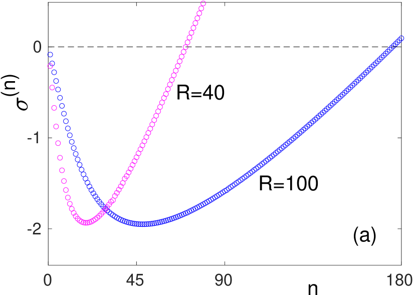
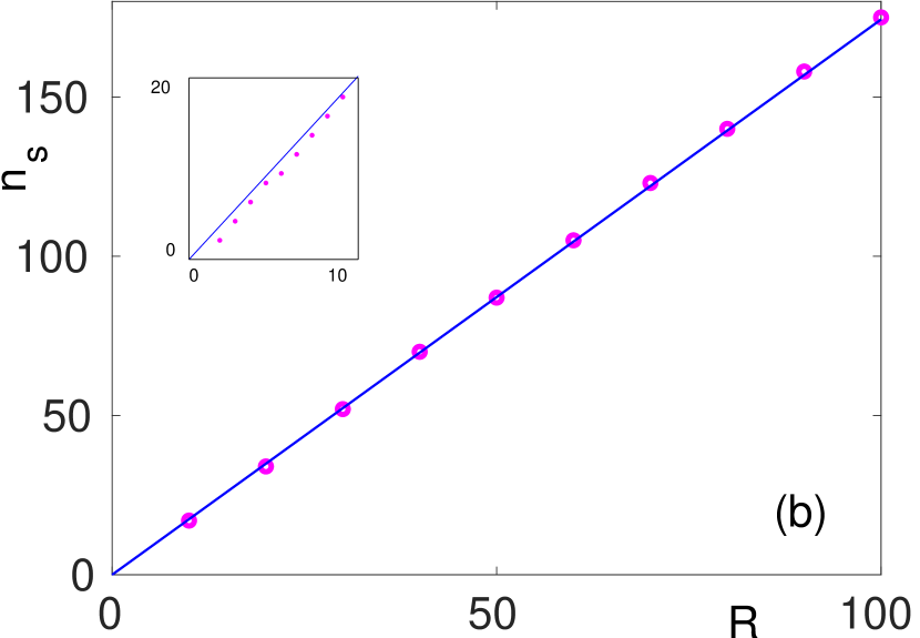
Figure 1: (a) The integral (14) for $R=40$ and $R=100$. The function $\sigma^{(n)}$ is negative for all $n\leq n_{s}(R)$ and positive for $n>n_{s}(R)$. (b) The integer $n_{s}$ (marked by circles) for a sequence of $R$ values. For $R\geq 2$, the function $n_{s}(R)$ is well approximated by $n_{s}=(\sqrt{30}/\pi)R$ (shown by the straight line). The inset blows up the interval $2\leq R<10$.

The values of the integral (14) with varied $n$ are presented graphically in Fig 1. The quantity $\sigma^{(n)}$ is determined to be negative for all $n\leq n_{s}$ and positive for $n>n_{s}$, where $n_{s}$ is an integer dependent on $R$. When $R$ is large enough, a fairly accurate approximation for $n_{s}(R)$ is given by the integer part of $(\sqrt{30}/\pi)R$.

The general solution of the amplitude equation (13) is

$$A=\exp\left(i\frac{3\sigma^{(n)}}{\Omega^{(n)}R}\mathcal{T}_{2}\right),$$ (15)

where the initial value was set equal to 1. (There is no loss of generality in setting $A(0)$ to 1 as it enters $\phi_{n}$ only in combination $\epsilon A(0)$, where $\epsilon$ is free to vary.) Thus, the fundamental frequency of the Bessel wave with amplitude $\epsilon$, branching off the trivial solution $\phi=0$ at the point $\omega=\Omega^{(n)}$, is

$$\omega=\Omega^{(n)}+\frac{3\sigma^{(n)}}{\Omega^{(n)}R}\epsilon^{2}+....$$ (16)

Note that the nonlinear frequency shift is negative ($\omega<\Omega^{(n)}$) for all $n\leq n_{s}$ and positive for $n>n_{s}$.

The relation (16) implies that our $\epsilon$-expansion is, in fact, an expansion in powers of the detuning from the resonant frequency, $|\omega-\Omega^{(n)}|$.

The energy (3) of the series solution (6) is

$$E^{(n)}(\epsilon)=4\pi R\left(\Omega^{(n)}\right)^{2}\epsilon^{2}+O(\epsilon^{4}).$$ (17)

Eliminating $\epsilon^{2}$ between (16) and (17) we can express the energy of the Bessel wave as a function of its frequency:

$$E^{(n)}(\omega)=\frac{4\pi R^{2}\left(\Omega^{(n)}\right)^{3}}{3\sigma^{(n)}}\left(\omega-\Omega^{(n)}\right)+O\left(\left(\omega-\Omega^{(n)}\right)^{2}\right).$$ (18)

This is an equation of a ray emanating from the point $(\Omega^{(n)},0)$ on the $(\omega,E)$, $E>0$, half-plane. The slope of the ray is negative for all $n\leq n_{s}(R)$ and positive for $n>n_{s}(R)$.

All solutions of equation (13) are stable. (Trajectories form concentric circles on the $(\mathrm{Re}A,\mathrm{Im}A)$ phase plane.)

The asymptotic construction of the Bessel wave is corroborated by the numerical analysis of the boundary-value problem (2). A numerically-continued branch starting with the trivial solution $\phi=0$ at $\omega=\Omega^{(n)}$ consists of standing waves with $n-1$ nodes inside the interval $(0,R)$. An important feature of these solutions is their weak localisation. Even when the energy of the Bessel wave is high — that is, even when the solution is far from its linear limit (9) — the wave does not have an exponentially localised core and the amplitude of the damped sinusoid $\phi(r,t)$ remains of order $R^{-1}$ as $r$ approaches $R$. (See Fig 2.)

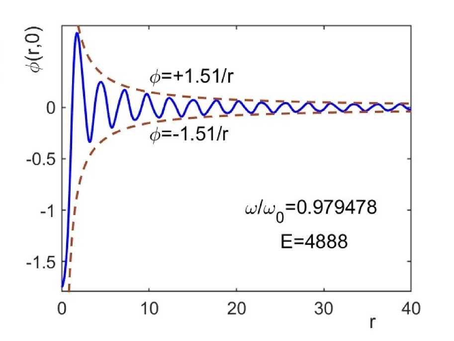
Figure 2: A snapshot of the Bessel wave with high energy. This solution was obtained by the numerical continuation of the trivial solution from $\omega=\Omega^{(114)}$, in a ball with $R=150$. (For the entire Bessel branch see Fig 7.) The wave is depicted by a solid line while its dashed envelope highlights the absence of a well-defined core. Note that only a portion of the $(0,150)$ interval is shown.

Consistently with the asymptotic considerations, the numerically continued Bessel waves are stable near their inception points and only lose stability as their energies become high enough. (For details of the corresponding period-doubling bifurcation see section IV.1.)

The continuation starting at the lowest of the resonance values, $\omega=\Omega^{(1)}$, produces a stable branch with a steep negative slope (Fig 3). The steep growth of the energy is due to the small absolute value of $\sigma^{(1)}$ in (18) while the negativity of $dE^{(1)}/d\omega$ is due to $n_{s}(100)$ being greater than 1. As the solution is continued to lower values of $\omega$, the function $E(\omega)$ reaches a maximum and starts decreasing. Not unexpectedly, the asymptotic expansion in powers of the small detuning $|\omega-\Omega^{(1)}|$ does not capture the formation of the energy peak.

Before turning to an asymptotic expansion about a different frequency value, we make a remark on the nomenclature of numerical solutions. Assume that the computation interval $(0,T)$ includes an integer number of fundamental periods of a solution of the boundary-value problem (2): $T=mT_{\mathrm{f}}$, $m>1$. Equation (4) gives then a formal frequency $\omega=\omega_{\mathrm{f}}/m$, where $\omega_{\mathrm{f}}=2\pi/T_{\mathrm{f}}$ is the fundamental frequency of the wave. In this case the periodic solution $\phi(r,t)$ will be referred to as the $1/m$ undertone of the standing wave.

It is important to emphasise that the only difference between a standing wave and its undertone is the length of the interval $(0,T)$ that we use to determine the respective solution — and hence its formal frequency (4). For example, the $n$-th Bessel wave is born with the frequency $\omega=\Omega^{(n)}$ while its $1/2$ undertone is born with $\omega=\Omega^{(n)}/2$. Basically, the $1/2$ undertone of the periodic oscillation $\phi(r,t)$ is the oscillation itself, where we skip every other beat.

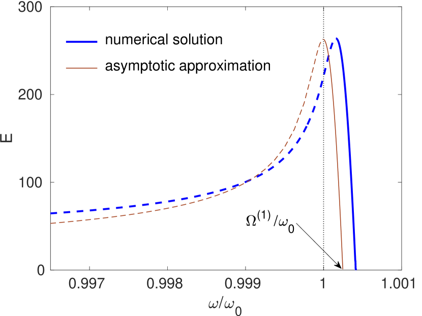
Figure 3: The $E(\omega)$ dependence near the point of inception of the standing wave in a ball with $R=100$. Blue (thick) curve: result of numerical continuation. Brown (thin) curve: asymptotic approximation exploiting $R^{-1}$ as a small parameter. Stable solutions are marked by the solid and unstable ones by the dashed lines.

III Small-amplitude wave in a large ball

III.1 Inverse radius as a small parameter

In order to account for the energy peak in Fig 3 and track the $E(\omega)$ curve over the point of maximum analytically, we need an asymptotic expansion of a different kind. Instead of assuming the proximity to the resonant frequency $\omega=\Omega^{(1)}$, we will zoom in on the neighbourhood of the frequency $\omega_{0}$ corresponding to the uniform oscillations in an infinitely large ball. Our approach is a relative of the Lindstedt-Poincare method utilised in the context of the infinite space in Ref Voronov2 ; B and elucidated in Fodor2 . (The method was pioneered in the one-dimensional setting Kose ; Dashen .)

We construct the small-amplitude solution in a ball of a large — yet finite — radius. Instead of the techniques used in Voronov2 ; B ; Fodor2 ; Kose ; Dashen , we employ a multiple scale expansion. This approach affords information on the spectrum of small perturbations of the standing wave, in addition to the standing wave itself.

The inverse radius $\epsilon=R^{-1}$ provides a natural small parameter. We expand $\phi$ as in (6), introduce the sequence of slow times $\mathcal{T}_{n}$ and, in addition, define a hierarchy of spatial scales ${\bf X}_{n}=\epsilon^{n}{\bf x}$. Hence

$$\nabla=\nabla_{0}+\epsilon\nabla_{1}+\epsilon^{2}\nabla_{2}+...,\quad\nabla_{n}=\frac{\partial}{\partial{\bf X}_{n}}.$$

These expansions are substituted in the equation (2a) where, for ease of computation, we drop the requirement of spherical symmetry:

$$\phi_{tt}-\nabla^{2}\phi+2\phi-3\phi^{2}+\phi^{3}=0.$$ (19)

At the order $\epsilon^{1}$, we choose a spatially homogeneous solution

$$\phi_{1}=Ae^{i\omega_{0}\mathcal{T}_{0}}+c.c.$$ (20)

In (20), the amplitude $A$ does not depend on ${\bf X}_{0}$ or $\mathcal{T}_{0}$ but may depend on the “slower” variables ${\bf X}_{1},{\bf X}_{2},...$ and $\mathcal{T}_{1},\mathcal{T}_{2},...$.

The order $\epsilon^{2}$ gives

$$\phi_{2}=3|A|^{2}-\frac{1}{2}A^{2}e^{2i\omega_{0}\mathcal{T}_{0}}+c.c.,$$ (21)

and we had to impose the constraint $\partial A/\partial\mathcal{T}_{1}=0$. Proceeding to the cubic order in $\epsilon$ we obtain

$$\left(\frac{\partial^{2}}{\partial\mathcal{T}_{0}^{2}}-\nabla_{0}^{2}+2\right)\phi_{3}=-4A^{3}e^{3i\omega_{0}\mathcal{T}_{0}}+c.c.$$

$$+\left(\nabla_{1}^{2}A-2i\omega_{0}\frac{\partial A}{\partial\mathcal{T}_{2}}+12|A|^{2}A\right)e^{i\omega_{0}\mathcal{T}_{0}}+c.c.$$ (22)

Setting to zero the secular term in the second line of (22), we arrive at the amplitude equation

$$-2i\omega_{0}\frac{\partial A}{\partial\mathcal{T}_{2}}+\nabla_{1}^{2}A+12|A|^{2}A=0.$$ (23a)

The boundary condition $$\phi(R,t)=0$$ translates into

$$\left.A({\bf X}_{1},\mathcal{T}_{2})\right|_{|{\bf X}_{1}|=1}=0.$$ (23b)

III.2 Schrödinger equation in a finite ball

A family of spherically-symmetric solutions of (23) is given by

$$A=e^{i\omega_{2}\mathcal{T}_{2}}\mathcal{R}_{\mu}(r_{1}),$$ (24)

where $r_{1}=\sqrt{{\bf X}_{1}^{2}}$ and $\mathcal{R}_{\mu}(\rho)$ solves the boundary-value problem

$$\mathcal{R}^{\prime\prime}+\frac{2}{\rho}\mathcal{R}^{\prime}+\mu\mathcal{R}+12\mathcal{R}^{3}=0,$$ (25a)

$$\mathcal{R}^{\prime}(0)=\mathcal{R}(1)=0,$$ (25b)

with $\mu=2\omega_{0}\omega_{2}$. (In (25), the prime stands for the derivative with respect to $\rho$.) In what follows we confine our attention to the nodeless (everywhere positive) solution $\mathcal{R}_{\mu}(\rho)$ (Fig 4). Of particular importance will be its norm squared,

$$N(\mu)=\int_{0}^{1}\mathcal{R}_{\mu}^{2}(\rho)\rho^{2}d\rho.$$ (26)

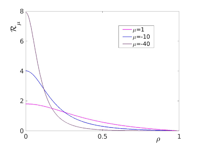
Figure 4: $\mathcal{R}_{\mu}(\rho)$: the nodeless solution of the boundary-value problem (25). As $\mu$ changes from negative to positive values, the exponentially localised solution gives way to a function without a clearly defined core.

The nodeless solution $\mathcal{R}_{\mu}(\rho)$ exists for all $\mu$ with $-\infty<\mu<\pi^{2}$. As $\mu\to\pi^{2}$, a perturbation argument gives

$$\mathcal{R}_{\mu}(\rho)=\alpha\sqrt{\pi^{2}-\mu}\,\frac{\sin(\pi\rho)}{\rho}+O\left((\pi^{2}-\mu)^{\frac{3}{2}}\right),$$ (27a)

$$\alpha^{2}=\frac{1}{12\pi}\frac{1}{2\mathrm{Si}(2\pi)-\mathrm{Si}(4\pi)}=1.973\times 10^{-2},$$ (27b)

so that the norm decays to zero:

$$N(\mu)=\frac{\alpha^{2}}{2}(\pi^{2}-\mu)+O\left(\left(\pi^{2}-\mu\right)^{2}\right).$$

As $\mu\to-\infty$, we have

$$\mathcal{R}_{\mu}(\rho)\to\sqrt{-\mu}\,S\left(\sqrt{-\mu}\rho\right),$$ (28)

where $S(\rho)$ is the nodeless solution of the boundary value problem

$$S^{\prime\prime}+\frac{2}{\rho}S^{\prime}-S+12S^{3}=0,$$ (29a)

$$S^{\prime}(0)=S(\infty)=0.$$ (29b)

Accordingly, the norm (26) decays to zero in the latter limit as well:

$$N(\mu)\to\frac{1}{\sqrt{-\mu}}\int_{0}^{\infty}S^{2}(\rho)\rho^{2}d\rho\quad\mbox{as}\ \mu\to-\infty.$$

The numerical analysis of the problem (25) verifies that $N(\mu)$ has a single maximum, at $\mu_{c}=-0.225$.

Thus we have constructed an asymptotic standing-wave solution of equation (2), parametrised by its frequency $\omega$:

$$\phi=\frac{2}{R}\cos(\omega t)\mathcal{R}_{\mu}\left(\frac{r}{R}\right)+O(R^{-2}),$$ (30a)

where

$$\mu=2\omega_{0}R^{2}(\omega-\omega_{0}).$$ (30b)

Substituting (30a) in (3) we obtain the corresponding energy:

$$E(\omega)=16\pi RN(\mu)+O(R^{-1}).$$ (31)

The dependence (31) is shown by the thin line in Fig 3. Unlike the expansion in powers of the frequency detuning (section II), the expansion in powers of $R^{-1}$ is seen to reproduce the energy peak. The peak of the curve $E(\omega)$ is a scaled version of the peak of $N(\mu)$.

Finally, we note that the function $\mathcal{R}_{\mu}(\rho)$ with negative $\mu$ has an exponentially localised core, with the width of the order $\frac{1}{\sqrt{-\mu}}$. By contrast, solutions with $\mu>0$ approach zero at a nearly uniform rate (Fig 4).

III.3 Stability of small-amplitude standing wave

By deriving the amplitude equation (23) the analysis of stability of the time-periodic standing wave has been reduced to the stability problem for the stationary solution of the 3D nonlinear Schrödinger equation. The leading order of a linear perturbation to the solution (30) is given by

$$\delta\phi=\left\{e^{i\omega_{0}\left(1+\frac{\mu}{4R^{2}}\right)t}\left[\mathcal{F}\left(\frac{r}{R}\right)+i\mathcal{G}\left(\frac{r}{R}\right)\right]+c.c.\right\}$$

$$\times\exp\left(\frac{\lambda}{2\omega_{0}R^{2}}t\right),$$ (32)

where $\mathcal{F}=\mathcal{F}(\rho)$ and $\mathcal{G}=\mathcal{G}(\rho)$ are two components of an eigenvector of the symplectic eigenvalue problem

$$L_{0}\mathcal{G}=-\lambda\mathcal{F},\quad L_{1}\mathcal{F}=\lambda\mathcal{G}.$$ (33)

In (33), $L_{0}$ and $L_{1}$ are a pair of radial operators

$$L_{0}=-\frac{d^{2}}{d\rho^{2}}-\frac{2}{\rho}\frac{d}{d\rho}-\mu-12\mathcal{R}_{\mu}^{2}(\rho),$$

$$L_{1}=-\frac{d^{2}}{d\rho^{2}}-\frac{2}{\rho}\frac{d}{d\rho}-\mu-36\mathcal{R}_{\mu}^{2}(\rho),$$ (34)

with the boundary conditions

$$\mathcal{F}^{\prime}(0)=\mathcal{G}^{\prime}(0)=\mathcal{F}(1)=\mathcal{G}(1)=0.$$ (35)

The lowest eigenvalue of the Schrödinger operator $L_{0}$ is zero, with the associated eigenfunction given by $\mathcal{R}_{\mu}(\rho)$. Numerical analysis reveals that the operator $L_{1}$ has a single negative eigenvalue. This is the case of applicability of the Vakhitov-Kolokolov criterion VK ; Peli1 ; Peli2 . The criterion guarantees the stability of the solution (24) if $dN/d\mu<0$ and instability otherwise.

Numerical methods confirm that in the region $\mu_{c}<\mu<\pi^{2}$, the eigenvalue problem (33)-(35) does not have any real eigenvalues apart from a pair of zeros resulting from the U(1) invariance of (23a). (We remind that $\mu_{c}$ is the point of maximum of the curve $N(\mu)$; $\mu_{c}=-0.225$.) As $\mu$ is decreased through $\mu_{c}$, a pair of opposite pure-imaginary eigenvalues $\pm\lambda_{0}(\mu)$ converges at the origin and diverges along the positive and negative real axis. As $\mu\to-\infty$, the scaling (28) gives $\lambda_{0}(\mu)\to-5.50\mu$, where $5.50$ is the symplectic eigenvalue associated with the solution of the infinite domain problem (29).

The upshot of our asymptotic analysis is that there is a continuous family of standing-wave solutions in the ball of a large radius $R$, with frequencies $\omega$ extending down from $\Omega^{(1)}$. The function $E(\omega)$ features a sharp peak at $\omega_{c}=\omega_{0}+\mu_{c}(2\omega_{0}R^{2})^{-1}$, with the standing waves to the right of the peak (where $dE/d\omega<0$) being stable and those to the left (where $dE/d\omega>0$) unstable. (See the thin curve in Fig 3.)

III.4 Continuation over the energy peak

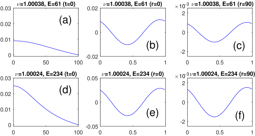
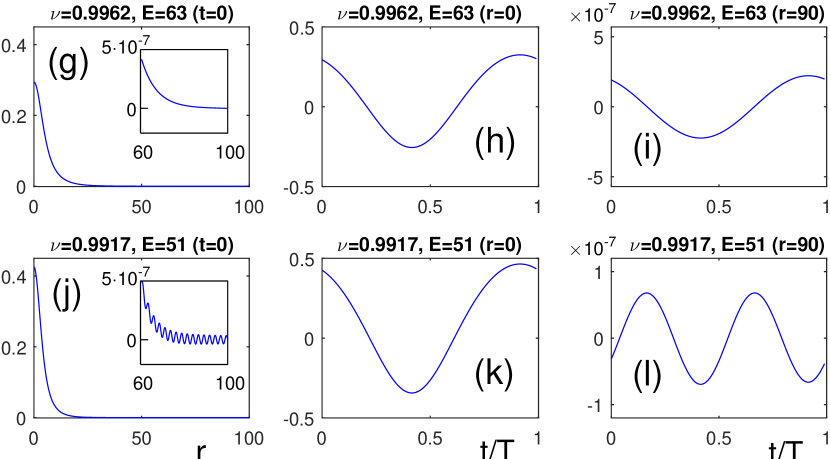
Figure 5: Top to bottom row: standing wave as it is continued from $\Omega^{(1)}$ to lower $\omega$ in Fig 3. (The ball radius $R=100$.) Left column: spatial profile at a particular time, $\phi(r,0)$. Middle and right column: temporal behaviour at the central and a peripheral point, $\phi(0,t)$ and $\phi(90,t)$. In the panel legends, $\nu$ is the normalised frequency: $\nu=\omega/\omega_{0}$. The same notation is used in Figs 8, 10, 11

The large-$R$ perturbation expansion with $\omega$ close to $\omega_{0}$ was validated by the numerical study of the boundary-value problem (2). We continued the periodic solution $\phi(r,t)$ to lower $\omega$ and used the linearised equation (5) to evaluate the associated monodromy matrix. In agreement with the asymptotic considerations, a pair of real Floquet multipliers ($\zeta$ and $\zeta^{-1}$) was seen to leave the unit circle as $\omega$ passed through the point of maximum energy. Consequently, the left slope of the energy peak in Fig 3 does indeed correspond to unstable standing waves.

Fig.5 documents the solution as it is continued from $\Omega^{(1)}$ over the energy peak. Consistently with the asymptotic expression (30), the peripheral field values $\phi(r_{p},t)$, where $r_{p}\sim R$, oscillate at the same frequency $\omega$ as the amplitude at the origin, $\phi(0,t)$. This agreement is recorded on either side of the energy peak; see panel pairs (b) and (c), (e) and (f), (h) and (i).

As $\omega$ is reduced below the point of maximum energy, the Bessel-function profile (30), (27) gives way to an exponentially localised shape. This metamorphosis agrees with the evolution of the asymptotic profile $\mathcal{R}_{\mu}(\rho)$ as $\mu$ is taken from positive to negative values. The difference in the type of decay is clearly visible in panels (a), (d) and (g) of Fig 5. Lowering $\omega$ even further sees the formation of a small-amplitude undulating tail (Fig 5(j)). At the same time, the oscillation frequency in the peripheral region switches from the frequency of the core of the standing wave to its second harmonic (compare panel (l) to (k)).

It may seem that the presence of the second-harmonic tail is at variance with the uniformly-first harmonic pattern (30). There is no contradiction, in fact. As we take $\omega$ far enough from $\omega_{0}$, the assumption $\phi=O(R^{-1})$ becomes invalid and the expression (30) stops providing any accurate approximation to the solution $\phi(r,t)$.

Why does the formation of the second-harmonic tail require taking $\omega$ far from $\omega_{0}$? The reason is that when $\omega$ is close to $\omega_{0}$, the core of the exponentially-localised standing wave is much wider than the wavelength of the second-harmonic radiation:

$$\frac{1}{\sqrt{2\omega_{0}(\omega_{0}-\omega)}}\gg\frac{2\pi}{\sqrt{3\omega_{0}^{2}}}.$$

(Here we took advantage of the fact the characteristic width of the bell-shaped function $\mathcal{R}_{\mu}(\rho)$ is $1/\sqrt{-\mu}$ and used (30b) to express $\mu$.) As a result, the radiation coupling to the core is weak and its amplitude is exponentially small. Thus when $\omega$ is close to $\omega_{0}$, we can simply not discern the amplitude of the second harmonic against the first-harmonic oscillation.

III.5 Small-amplitude wave in the infinite space

It is instructive to comment on the $R\to\infty$ limit for which the small-amplitude solution is available in the earlier literature Voronov2 ; B ; Fodor2 .

In the case of the infinitely large ball our asymptotic expansion remains in place but $\epsilon$ becomes a formal expansion parameter, not tied to $R$. Without loss of generality, we can let $\mu=-1$ in equation (25a) while the boundary condition $\mathcal{R}(1)=0$ should be replaced with $\mathcal{R}(\infty)=0$. In agreement with Voronov2 ; B ; Fodor2 , the asymptotic solution (6) acquires the form

$$\phi=2\epsilon\cos\left[\omega_{0}\left(1-\frac{\epsilon^{2}}{4}\right)t\right]S(\epsilon r)+O(\epsilon^{2}),$$ (36)

where $\mathcal{S}(\rho)$ is a nodeless solution of the boundary value problem (29). (For solutions of (29) see Anderson ; Fodor2 .) As $\omega\to\omega_{0}$ (i.e. as $\epsilon\to 0$), the energy of the asymptotic solution (36) tends to infinity:

$$E=\frac{16\pi}{\epsilon}\int_{0}^{\infty}S^{2}(\rho)\rho^{2}d\rho=\frac{16\pi}{\epsilon}\times 0.1253.$$ (37)

Stability or instability of the infinite-space solution is decided by eigenvalues of the symplectic eigenvalue problem (33)-(34) with $\mu$ set to $-1$, $\mathcal{R}_{\mu}(\rho)$ replaced with $S(\rho)$, and the boundary conditions (35) substituted with $\mathcal{F}(\infty)=\mathcal{G}(\infty)=0$. The numerical analysis verifies that the resulting symplectic problem has a (single) pair of opposite real eigenvalues $\lambda=\pm 5.50$. Hence the solution (36) is unstable for any sufficiently small $\epsilon$.

IV Resonances in the ball

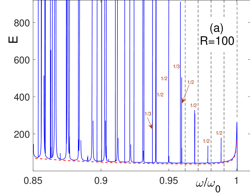
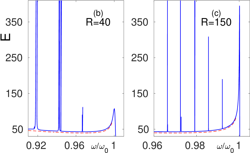
Figure 6: (a) Energy of the standing wave with frequency $\omega$ in the ball of radius $R=100$ (a), $R=40$ (b) and $R=150$ (c). The $E(\omega)$ curve features a sequence of sharp spikes that have complex fine structure indiscernible in the figure. Although some branches were only continued to moderate energies, we expect all spikes to extend to the top of the panels. The vertical dashed lines in (a) mark the points $\omega=\Omega^{(n)}/2$ where $\Omega^{(n)}$ are the frequencies of the newborn Bessel waves (defined by equation (8)). The fraction next to a spike indicates the order of the Bessel-wave undertone that this spike’s slopes approach (but not necessarily join) at a larger $E$. (The Bessel undertones are not shown in the figure.) In all three panels, the red dashed arc underlying the $E(\omega)$ curve is the envelope of the family of spikes. For visual clarity, it has been shifted down by a tiny amount from its actual position.

IV.1 Energy-frequency diagram

The numerical continuation beyond the peak in Fig 3, from right to left, produces an $E(\omega)$ curve with what looks like a sequence of spikes. Fig 6(a) depicts this curve for $R=100$. It also shows an envelope of the family of spikes — a U-shaped arc that coincides with the $E(\omega)$ curve everywhere except the neighbourhoods of the spikes. In the neighbourhood of each spike, the envelope bounds it from below.

Figs 6(b) and (c) compare the density of spikes in the diagrams with different values of $R$. (Either panel focusses on the right end of the respective diagram where spikes are thin and nonoverlapping.) The number and positions of the spikes are seen to be $R$-sensitive. In contrast, the U-shaped envelope does not change appreciably as the radius of the ball is varied. Regardless of $R$, the U-shaped curve has a single minimum, at

$$\omega_{\mathrm{min}}=0.967\,\omega_{0}.$$ (38)

The U-shaped envelope agrees with the energy curve of periodic infinite-space solutions with exponentially localised cores and small-amplitude tails decaying slowly as $r\to\infty$ Fodor1 . The energy of those nanopterons is defined as the integral (3) where $R$ is a radius of the core. The nanopteron’s energy has a minimum at $\omega=0.9652\,\omega_{0}$ Fodor1 which is close to our $\omega_{\mathrm{min}}$ in (38).

A sequence of vertical dashed lines drawn at $\omega=\frac{1}{2}\Omega^{(n)}$ in Fig 6(a) is seen to match the sequence of spikes. The correspondence between the two sequences suggests some relation between the spikes and the Bessel waves born at $\omega=\Omega^{(n)}$.

IV.2 Bifurcation unpacked

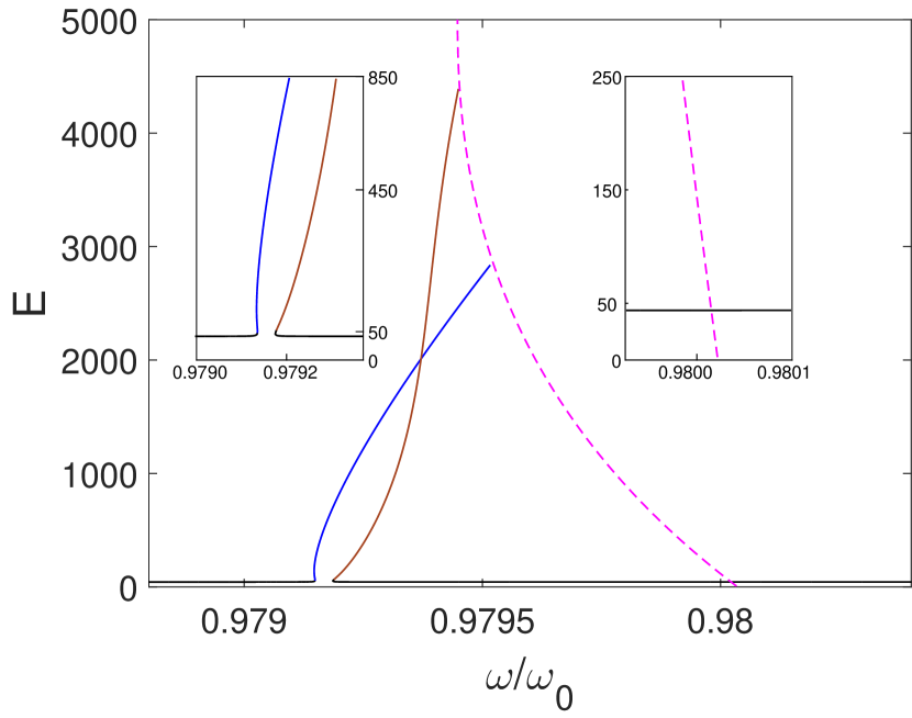
Figure 7: A fragment of the $E(\omega)$ diagram in the vicinity of a 1:2 resonance in the ball with $R=150$. The blue and brown curves are two slopes of the “spike”. The dashed magenta arc emerging from $E=0$ at $\omega=\Omega^{(114)}/2$ is the $1/2$ undertone of the $n=114$-th Bessel wave, (That is, a point $(\omega,E)$ on this branch represents the Bessel wave with frequency $2\omega$.) The insets zooming in on the lower sections of the “spike” and Bessel branch aim to emphasise the difference in the origins of the two branches.

Zooming in on one of the distinctly separate spikes near the right end of the diagram reveals that it is not a mere peak, or projection, on the $E(\omega)$ curve. As in a proper peak, there are two energy branches that rise steeply from the U-shaped arc but instead of joining together, the left and right “slopes” connect to another curve. This curve turns out to be a Bessel branch — more precisely, the $1/2$ undertone of the Bessel branch emerging from $\phi=0$ at the frequency $\omega=\Omega^{(n)}/2$ with some large $n$ (Fig 7).

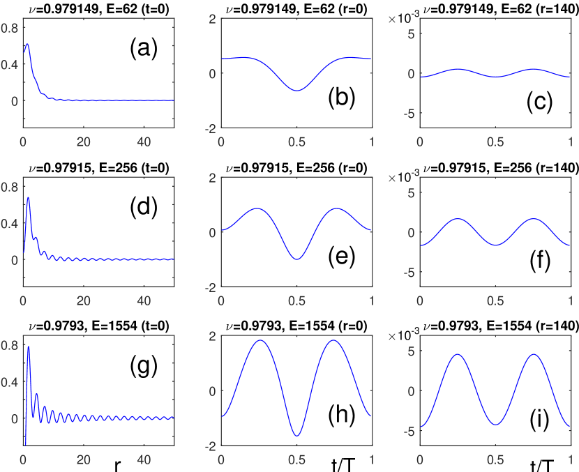
Figure 8: Top to bottom row: spatial and temporal behaviour of the solution to the problem (2) as it is continued along the blue slope of the “spike” in Fig 7, from the underlying U-arc towards the Bessel curve. Left column: snapshot of $\phi(r,t)$ at a particular moment of time ($t=0$); central column: behaviour of the central value $\phi(0,t)$; right column: evolution of an asymptotic value $\phi(r_{p},t)$ with $r_{p}=140$. All solutions satisfy the boundary condition $\phi(150,t)=0$.

To appreciate details of the bifurcation, we follow the curve corresponding to the left slope of the “spike” (the blue curve in Fig 7). A standing wave with $(\omega,E)$ located at the base of the “spike” has an exponentially localised core and an oscillatory tail with the amplitude decaying in proportion to $r^{-1}$ (Fig 8(a)). The $\phi$-value at $r=0$ performs nearly-harmonic oscillations with the fundamental frequency $\omega={2\pi}/{T}$ (panel (b)) while the tail oscillates at the frequency $2\omega$ (panel (c)).

Moving up the blue curve in Fig 7, the contribution of the second harmonic to the oscillation of the core increases (Fig 8(e)). Eventually, when the curve is about to join the branch of the $1/2$ Bessel undertones (shown by the dashed magenta in Fig 7), $\phi(0,t)$ completes two nearly-identical cycles over the interval $T=2\pi/\omega$ (Fig 8(h)). The solution does not have any well-defined core (panel (g)), with the central and peripheral values oscillating at the same fundamental frequency $2\omega$ (panels (h) and (i)). This is exactly the spatio-temporal behaviour of the $1/2$ Bessel undertone.

Note that the merger of the blue and magenta curves in Fig 7 can be seen as the period-doubling bifurcation of the Bessel wave. As we observed in section II, the $n$-th Bessel wave ($n=1,2,...$) is stable when its frequency is close enough to $\Omega^{(n)}$, its inception point. Our numerical analysis indicates that the Bessel wave loses its stability once its energy $E$ has grown above the period-doubling bifurcation value. A quadruplet of complex Floquet multipliers leaves the unit circle at this point signifying the onset of instability against an oscillatory mode with an additional frequency.

While most of the clearly distinguishable, nonoverlapping, spikes result from the 1:2 resonances with the Bessel waves, some correspond to the 1:3, 1:4 or 1:6 resonances. Similar to the 1:2 spikes, an exponentially localised solution at the base of a 1:3, 1:4 or 1:6 projection has a core oscillating at the frequency $\omega=2\pi/T$ and its second-harmonic tail. As this solution is continued up the slope of its spike, the contribution of higher harmonics to the oscillation of the core and tail increases. Eventually the standing wave switches to the uniform regime where its core and tail oscillate at the same frequency — $3\omega$, $4\omega$ or $6\omega$. The change of the temporal pattern is accompanied by the transformation of the spatial profile of the wave, from the “core-and-tail” composition to a slowly decaying structure with no clearly defined core.

It would be natural to expect this weakly localised solution to merge with the 1/3, 1/4 or 1/6 undertone of a Bessel wave, implying the period multiplication of the latter. Numerically, we do observe the bifurcations with $m=4$ and 6 while the period-tripling of a Bessel wave is yet to be discovered.

IV.3 Higher resonances

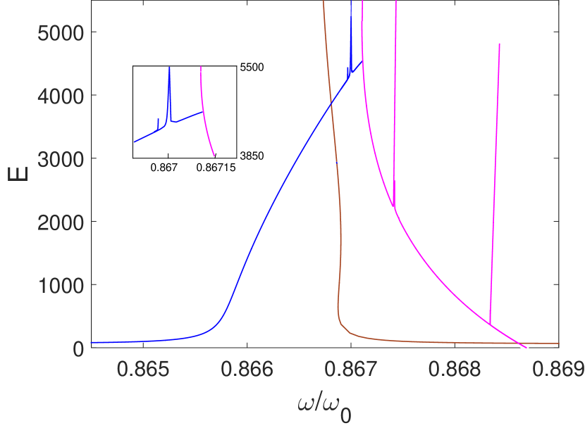
Figure 9: The bifurcation diagram in the neighbourhood of $\omega=\Omega^{(64)}/2$ in the ball of radius $R=100$. The inset zooms in on a tiny segment of the left slope of the primary peak (blue curve) that hosts two baby spikes and merges with the Bessel branch (shown in magenta).

Fig 9 zooms in on the neighbourhood of $\omega=\Omega^{(64)}/2$ in the ball of radius $R=100$. Besides the primary spike pattern recognisable from our earlier Fig 7, the diagram features several thinner vertical projections. These secondary, or “baby”, spikes result from resonances with higher harmonics.

The magenta curve in Fig 9 comprises the $1/2$ undertones of the Bessel wave. This branch and two needlelike secondary projections sprouting up from it represent standing waves without clearly defined cores; see Fig 10. The top row in Fig 10 corresponds to a solution occurring between the two baby spikes; it consists of a pair of identical cycles on the interval $(0,2\pi/\omega)$. The middle row of Fig 10 exemplifies standing waves found on either slope of the “lower” baby spike (spike centred on $\omega/\omega_{0}=0.86834$). These include six repeated cycles. As $E$ grows, both slopes of the “lower” spike merge with the branch of the $1/6$ undertones of another Bessel branch extending from $E=0$ (not shown in Fig 9). Finally, in the bottom row of Fig 10 we display a solution that belongs to the secondary projection appearing higher on the Bessel curve (spike centred on $\omega=0.86741$). This coreless standing wave oscillates at the frequency $10\,\omega$.

We note that solutions on both slopes of each of the two baby spikes emerging from the Bessel branch are stable.

Fig 11 documents standing waves found on the left slope of the primary spike (the blue curve in Fig 9) and secondary spikes emerging from it. The top row illustrates the solution at a point of the primary curve near its merger with the Bessel branch. The structure of this solution is similar to that in the bottom row of Fig 8. The wave does not have a clearly defined core while its central value $\left.\phi\right|_{r=0}$ and a slowly decaying tail oscillate at the same frequency $2\,\omega$. The middle and bottom rows in Fig 11 describe solutions on the left and right baby spikes jutting out from the primary curve. These have a large-amplitude $12\,\omega$- and $9\,\omega$-component, respectively.

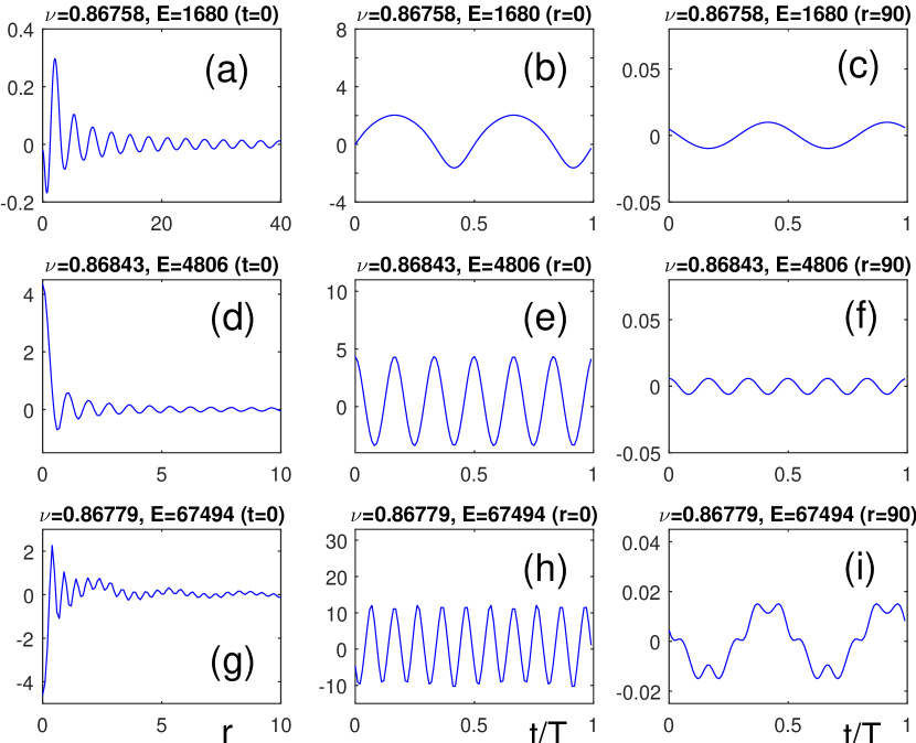
Figure 10: Solutions on the Bessel branch and its two offshoots in Fig 9. Top row: the wave of frequency $2\omega$ found on the Bessel curve between the two baby spikes. Middle row: solution of frequency $6\,\omega$ represented by the right-hand offshoot. Bottom row: solution of frequency $10\,\omega$ corresponding to the left baby spike.

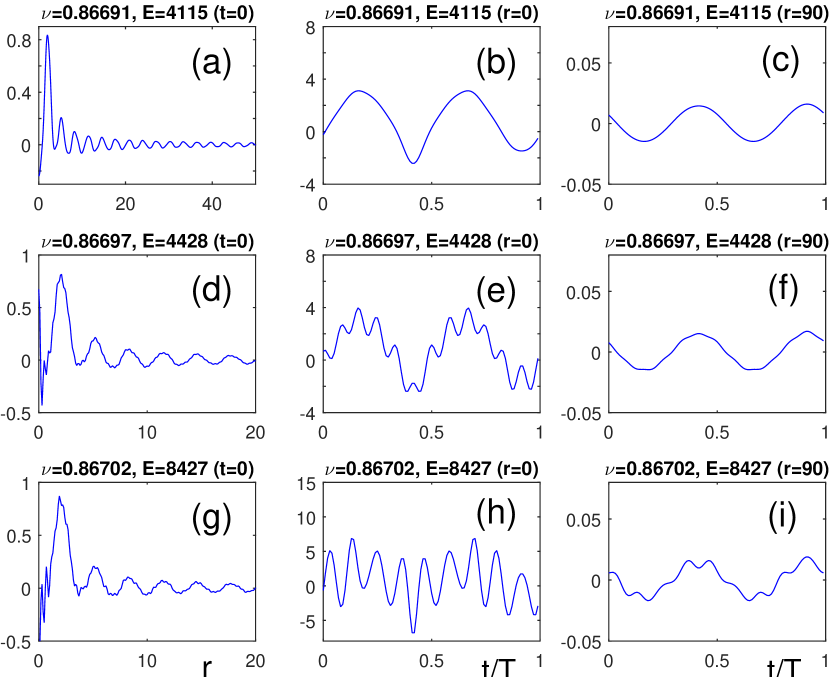
Figure 11: Top row: solution of frequency $2\omega$ on the blue side of the primary “peak” shown in Fig 9. Middle respectively bottom row: solutions of frequency $12\,\omega$ respectively $9\,\omega$ found on the left respectively right baby spike stemming out from the primary peak. (The two spikes are clearly visible in the inset to Fig 9). All three standing waves are coreless due to the proximity to the Bessel branch.

IV.4 Stability of standing waves

With the stability of the Bessel waves classified earlier in this paper, we turn to the exponentially localised solutions comprising the $E(\omega)$ curve in Fig 6.

As we demonstrated in sections III.3 and III.4, the monodromy matrix acquires a pair of real eigenvalues ($\zeta_{1}>1$ and $\zeta_{2}=1/\zeta_{1}$) as the solution is continued over the peak at $\omega_{c}=\omega_{0}+\mu_{c}(2\omega_{0}R^{2})^{-1}$ (the rightmost peak in Fig 6) in the direction of lower frequencies. The numerical analysis indicates that another real pair ($\zeta_{3}>1$ and $\zeta_{4}=1/\zeta_{3}$) leaves the unit circle as $\omega$ is reduced past the local energy minimum between the peak at $\omega_{c}$ and the next spike on its left.

Regardless of the choice of $R$, real or complex unstable Floquet multipliers persist over the entire interval $\omega_{\mathrm{min}}<\omega<\omega_{c}$, where $\omega_{\mathrm{min}}$ is the point of minimum of the U-shaped envelope of the family of spikes. For low energies, the instability is due to the real multipliers, $\zeta_{1}$ and $\zeta_{3}$. As the solution “climbs” up the energy slope, the real multipliers $\zeta_{1}$, $\zeta_{3}$, $1/\zeta_{1}$, $1/\zeta_{3}$ merge, pairwise, and form a complex quadruplet. The quadruplet dissociates as the solution descends along the other slope of the same spike.

Stability properties in the region $\omega<\omega_{\mathrm{min}}$ prove to be sensitive to the choice of $R$. The case of a small radius is exemplified by the ball of $R=40$. Fig 6(b) depicts the corresponding $E(\omega)$ diagram in an interval of frequencies adjacent to $\omega_{0}$. (Note that the frequency $\omega_{\mathrm{min}}$ is close to the position of the second spike from the right in Fig 6(b).)

All frequencies between each pair of spikes in Fig 6(b) correspond to unstable solutions, with one or two pairs of real Floquet multipliers off the unit circle. The second spike from the right (spike centred on $\omega\approx 0.97$) is also entirely unstable. The only intervals of stability in Fig 6(b) are found at the base of the third and forth spike (centred on $\omega\approx 0.94$ and $\omega\approx 0.92$, respectively). Fig 12(a) illustrates stability of several branches associated with the third spike.

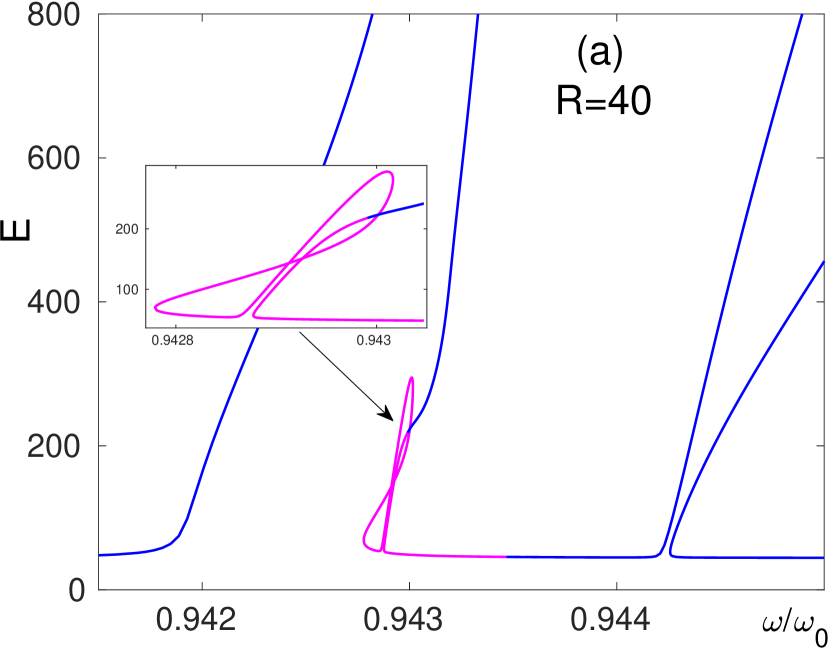
Figure 12: (a) The fine structure of the third spike from the right in Fig 6(b). (Here $R=40$.) The spike is, in fact, a doublet; it consists of two separate projections. The inset zooms in on a figure-eight shaped isola occurring at the bottom of the left “subspike”. (b) Stability of standing waves in the ball of $R=100$, near the right end of its energy-frequency diagram (Fig 6(a)). In (a) and (b) the magenta respectively blue lines demarcate stable respectively unstable standing waves.

Turning to a larger ball radius ($R=100$), the stability domain expands considerably. As $\omega$ is reduced below $\omega_{\mathrm{min}}$ in that case, two pairs of real multipliers form a complex quadruplet which, on further reduction, converges to two points on the unit circle. The value of $\omega$ at which the multipliers join the circle marks the beginning of a sizeable interval of stable frequencies (Fig 12(b)). A continued reduction of $\omega$ sees an intermittent appearance and disappearance of one or several complex quadruplets separating stability from instability intervals.

V Concluding remarks

A linear standing wave in a ball results from the interference of an expanding spherical wavetrain of infinitesimal amplitude and the wavetrain reflected from the ball’s surface. When continued to finite amplitudes, the resulting nonlinear solution does not have a well-defined core and retains the $r$-dependence similar to the spherical Bessel function $j_{0}(r)=\frac{\sin r}{r}$. The total energy associated with this configuration in a ball of radius $R$ is a multiple of $R^{2}$.

A different type of nonlinear standing wave in a ball is characterised by an exponentially localised pulsating core. The core is a fundamentally nonlinear feature; the nonlinearity shifts its frequency below the linear spectrum and this frequency shift ensures the core’s exponential localisation. The core pulsating at the frequency $\omega$ radiates spherical waves with higher-harmonic frequencies $m\omega$, $m=2,3,...$. The standing pattern arises as a result of the interference of the expanding and reflected radiation wavetrains.

As the radiation frequency $m\omega$ comes near one of the linear eigenfrequencies, the solution approaches the corresponding Bessel-like pattern. The amplitude of the radiation increases and the total energy in the ball of radius $R$ shoots up to values $O(R^{2})$. By contrast, when $\omega$ is not near a resonant value, the radiation from the core is weak. The standing wave in that case may serve as an approximation to an oscillon — a long-lived localised pulsating structure in the infinite space — at the nearly-periodic stage of its evolution. Nonlinear standing waves provide information on the oscillon’s energy-frequency relation and stability as well as topology of the nearby regions of the phase space.

We examined the energy-frequency diagram of the standing wave and scrutinised the associated spatio-temporal transformation of the periodic solution. Results of this study can be summarised as follows.

1. We have demonstrated the existence of a countable set of standing waves (“Bessel waves”) in a ball of a finite radius. The $n$-th ($n=1,2,...$) Bessel wave is a solution of the boundary-value problem (2) with $n-1$ internal nodes in the interval $(0,R)$ and the envelope decaying in proportion to $r^{-1}$ as $r\to R$. The Bessel wave branches off the zero solution at $\omega=\Omega^{(n)}$; we have constructed it as an expansion in powers of the frequency detuning $\omega-\Omega^{(n)}$. The Bessel wave remains stable in an interval of frequencies adjacent to $\Omega^{(n)}$.

2. The nodeless ($n=1$) Bessel wave is amenable to asymptotic analysis in a wider frequency range. The pertinent asymptotic expansion is in powers of $R^{-1}$ and the resulting solution is valid in a neighbourhood of $\omega_{0}$, the frequency of spatially-uniform oscillations. This neighbourhood is found to be wide enough to include $\Omega^{(1)}$, the Bessel branch’s inception point, and $\omega_{c}$ ($\omega_{c}<\Omega^{(1)}$) — the frequency at which the energy curve $E(\omega)$ has a maximum. The $n=1$ Bessel wave remains stable in the entire interval $\omega_{c}\leq\omega<\Omega^{(1)}$ but loses its stability as $\omega$ is reduced below $\omega_{c}$.

3. The numerical continuation of the $n=1$ Bessel wave to values of $\omega$ below $\omega_{c}$ produces an $E(\omega)$ curve with a sequence of spikes near the undertone points $\omega=\Omega^{(n)}/2$ with some large $n$. The left and right slope of the spike adjacent to $\frac{1}{2}\Omega^{(n)}$ result from a period-doubling bifurcation of the $n$-th Bessel wave. In addition to the primary sequence $\frac{1}{2}\Omega^{(n)}$, there are also thinner spikes near the $\frac{1}{3}\Omega^{(n)}$, $\frac{1}{4}\Omega^{(n)}$ and other undertones. Slopes of the spikes in the primary sequence host secondary projections corresponding to higher resonances.

Away from the neighbourhoods of the spikes, the $E(\omega)$ curve follows a U-shaped arc with a single minimum at $\omega_{\mathrm{min}}=0.967\omega_{0}$; the arc bounds all spikes from below. The arc is unaffected by the ball radius variations, as long as $R$ remains large enough. This envelope curve describes the energy-frequency dependence of the nearly-periodic oscillons in the infinite space.

4. Standing waves with energies lying on the envelope curve and at the base of the spikes have an exponentially localised core and a small-amplitude slowly decaying second-harmonic tail. We have classified stability of these solutions against spherically-symmetric perturbations. Specifically, we focused on the interval $0.91\omega_{0}<\omega<\Omega^{(1)}$ and considered two values of $R$: $R=40$ and $R=100$. The ball of radius $R=40$ has only short stability intervals, located at the base of two spikes in its $E(\omega)$ diagram. By contrast, the standing waves in the ball of $R=100$ have long stretches of stable frequencies.

Finally, it is appropriate to draw parallels with resonance patterns observed in other systems.

The authors of Ref Morugante carried out numerical continuations of breather solutions in a one-dimensional necklace of Morse oscillators. Their $E(\omega)$ diagram features resonances similar to those reported in section IV of the present paper. Standing waves residing on the slopes of the spikes in our Figs 6, 7, 9 and 12(a) are akin to the phonobreathers of Ref Morugante while solutions represented by the U-arc in our Figs 6 correspond to their “phantom breathers”.

A more recent Ref Kev is a numerical study of the circular-symmetric breathers in the sine-Gordon equation posed in a disc of a finite radius. The $E(\omega)$ diagram produced in that publication displays projections due to the odd-harmonic resonances.

We note that neither Ref Morugante nor Kev observe a period-doubling transmutation of phonon waves into breathers.

References

References

- (1) N A Voronov, I Y Kobzarev, and N B Konyukhova, JETP Lett 22 290 (1975)
- (2) I L Bogolyubskii and V G Makhankov, JETP Lett 24 12 (1976)
- (3) I L Bogolyubskii and V G Makhankov, JETP Lett 25 107 (1977)
- (4) M Gleiser, Phys Rev D 49 2978 (1994)
- (5) E J Copeland, M Gleiser and H-R Müller, Phys Rev D 52 1920 (1995)
- (6) A Riotto, Phys Lett B 365 64 (1996)
- (7) I. Dymnikova, L. Koziel, M. Khlopov, and S. Rubin, Gravitation and Cosmology 6 311 (2000)
- (8) M. Broadhead and J. McDonald, Phys. Rev. D 72 043519 (2005)
- (9) M Gleiser, Int. J. Mod. Phys. D 16 219 (2007)
- (10) E. Farhi, N. Graham, A. H. Guth, N. Iqbal, R. R. Rosales, and N. Stamatopoulos Phys. Rev. D 77 085019 (2008)
- (11) M. Gleiser, B. Rogers, and J. Thorarinson, Phys. Rev. D 77 023513 (2008)
- (12) M. A. Amin, arXiv:1006.3075 (2010)
- (13) M Gleiser, N Graham, and N Stamatopoulos, Phys Rev D 83 096010 (2011)
- (14) M.A. Amin, R. Easther, H. Finkel, R. Flauger and M.P. Hertzberg, Phys. Rev. Lett. 108 241302 (2012)
- (15) S-Y Zhou, E J Copeland, R Easther, H Finkel, Z-G.Moua and P M Saffin, JHEP 10 026 (2013)
- (16) M Gleiser and N Graham, Phys Rev D 89 083502 (2014)
- (17) P. Adshead, J. T. Giblin Jr., T. R. Scully and E. I. Sfakianakis, Journ of Cosmology and Astroparticle Physics, 12 034 (2015)
- (18) J R Bond, J Braden and L Mersini-Houghton, Journ Cosmology and Astroparticle Physics 09 004 (2015)
- (19) S Antusch, F. Cefalà and S Orani, Phys Rev Lett 118 011303 (2017)
- (20) J-P Hong, M Kawasaki, and M Yamazaki, Phys Rev D 98 043531 (2018)
- (21) K. D. Lozanov and M. A. Amin, Phys. Rev. D 99 123504 (2019)
- (22) D Cyncynates and T Giurgica-Tiron, Phys Rev D 103 116011 (2021)
- (23) M Gleiser and J Thorarinson, Phys Rev D 76 041701(R) (2007)
- (24) V. Achilleos, F. K. Diakonos, D. J. Frantzeskakis, G. C. Katsimiga, X. N. Maintas, E. Manousakis, C. E. Tsagkarakis, and A. Tsapalis, Phys Rev D 88 045015 (2013)
- (25) V. A. Koutvitsky and E. M. Maslov, Phys Rev D 83 124028 (2011); Phys Rev D 102 064007 (2020); Phys Rev D 104 124046 (2021)
- (26) H-Y Zhang, Journ of Cosmology and Astroparticle Physics 03 102 (2021)
- (27) Z Nazari, M Cicoli, K Clough and F Muia, Journ of Cosmology and Astroparticle Physics 05 027 (2021)
- (28) X-X Kou, C Tian and S-Y Zhou, Class. Quantum Grav. 38 045005 (2021)
- (29) T Hiramatsu, E I Sfakianakis and M Yamaguchi, Journ High Energy Phys 21 2021 (2021)
- (30) X-X Kou, J B Mertens, C Tian and S-Y Zhou, Phys Rev D 105 123505 (2022)
- (31) E. W. Kolb and I. I. Tkachev, Phys. Rev. D 49 5040 (1994)
- (32) A Vaquero, J Redondo and J Stadler, Journ of Cosmology and Astroparticle Physics 04 012 (2019)
- (33) M Kawasaki, W Nakanoa, and E Sonomoto, Journ of Cosmology and Astroparticle Physics 01 047 (2020)
- (34) J Olle, O Pujolas, and F Rompineve, Journ of Cosmology and Astroparticle Physics 02 006 (2020)
- (35) M Kawasaki, K Miyazaki, K Murai, H Nakatsuka, E Sonomoto, Journ of Cosmology and Astroparticle Physics 08 066 (2022)
- (36) S Antusch, F Cefalà, S Krippendorf, F Muia, S Orani and F Quevedo, JHEP 01 083 (2018)
- (37) Y Sang and Q-G Huang, Phys. Rev. D 100 063516 (2019)
- (38) S Kasuya, M Kawasaki, F Otani, and E Sonomoto, Phys Rev D 102 043016 (2020)
- (39) E. Farhi, N. Graham, V. Khemani, R. Markov, R. Rosales, Phys. Rev. D 72 (2005) 101701(R);
- (40) N. Graham, Phys. Rev. Lett. 98 (2007) 101801; Phys. Rev. D 76 (2007) 085017;
- (41) M Gleiser, N Graham, and N Stamatopoulos, Phys Rev D 82 043517 (2010);
- (42) E. I. Sfakianakis, arXiv:1210.7568 (2012)
- (43) M.P. Hertzberg, Phys. Rev. D 82 045022 (2010)
- (44) P. M. Saffin, P. Tognarelli, and A. Tranberg, J. High Energy Phys. 08 125 (2014)
- (45) Sz. Borsányi and M. Hindmarsh, Phys Rev D 79 065010 (2009)
- (46) S. Kasuya, M. Kawasaki, and F. Takahashi, Phys. Lett. B 559 99 (2003)
- (47) M Kawasaki, F Takahashi, and N Takeda, Phys. Rev. D 92 105024 (2015)
- (48) K Mukaida, M Takimoto and M Yamada, JHEP 03 122 (2017)
- (49) M Ibe, M Kawasaki, W Nakano, and E Sonomoto, Phys Rev D 100 125021 (2019); JHEP 04 030 (2019)
- (50) E P Honda and M W Choptuik, Phys Rev D 65 084037 (2002)
- (51) M Gleiser and M Krackow, Phys Lett B 805 135450 (2020)
- (52) G Fodor, P Forgácz, P Grandclément, and I Rácz, Phys Rev D 74 124003 (2006)
- (53) M Gleiser and D Sicilia, Phys Rev Lett 101 011602 (2008)
- (54) M Gleiser and D Sicilia, Phys Rev D 80 125037 (2009)
- (55) M Gleiser, Phys Lett B 600 126 (2004)
- (56) G Fodor, P Forgácz, Z Horváth, Á Lukács, Phys Rev D 78 025003 (2008)
- (57) For each , equation (2a) was substituted with its second-order finite-difference discretisation in and . The numerical solutions in the ball of were obtained using the radial and temporal stepsizes and , respectively. The continuation in the and balls was carried out with and . The Floquet analyses used the forth-order Adams-Bashforth method for and the adaptive Runge-Kutta-Fehlberg algorithm for and .
- (58) R Grimshaw. Nonlinear Ordinary Differential Equations. Applied Mathematics and Engineering Science Texts, 2. Blackwell Scientific Publications, Oxford, 1990
- (59) C Chicone. Ordinary Differential Equations with Applications. Texts in Applied Mathematics, 34. Springer, New York, 2006
- (60) N A Voronov and I Y Kobzarev, JETP Lett 24 532 (1976)
- (61) I L Bogolyubskii, JETP Lett 24 579 (1976)
- (62) A M Kosevich and A S Kovalev, Sov Phys JETP 40 891 (1975)
- (63) R Dashen, B Hasslacher, and A Neveu, Phys Rev D 11 3424 (1975)
- (64) N.G. Vakhitov and A.A. Kolokolov, Radiophys. Quantum Electron. 16 783 (1973)
- (65) D.E. Pelinovsky, Proc. Roy. Soc. Lond. A 461 783 (2005)
- (66) M. Chugunova and D. Pelinovsky, Journ Math Phys 51 052901 (2010)
- (67) D L T Anderson and G H Derrick. Journ Math Phys 11 1336 (1970)
- (68) A M Morgante, M Johansson, S Aubry and G Kopidakis, J Phys A: Math Gen 35 4999 (2002)
- (69) P G Kevrekidis, R Carretero-González, J Cuevas-Maraver, D J Frantzeskakis, J-G Caputo, B A Malomed, Commun Nonlinear Sci Numer Simulat 94 105596 (2021)