Multipath-based SLAM for Non-Ideal Reflective Surfaces Exploiting Multiple-Measurement Data Association

Abstract

Multipath-based simultaneous localization and mapping (MP-SLAM) is a promising approach to obtain position information of transmitters and receivers as well as information regarding the propagation environments in future mobile communication systems. Usually, specular reflections of the radio signals occurring at flat surfaces are modeled by VAs that are mirror images of the physical anchors. In existing methods for MP-SLAM, each VA is assumed to generate only a single measurement. However, due to imperfections of the measurement equipment such as non-calibrated antennas or model mismatch due to roughness of the reflective surfaces, there are potentially multiple multipath components that are associated to one single VA. In this paper, we introduce a Bayesian particle-based sum-product algorithm (SPA) for MP-SLAM that can cope with multiple-measurements being associated to a single VA. Furthermore, we introduce a novel statistical measurement model that is strongly related to the radio signal. It introduces additional dispersion parameters into the likelihood function to capture additional MPC-related measurements. We demonstrate that the proposed SLAM method can robustly fuse multiple measurements per VA based on numerical simulations.

I Introduction

MP-SLAM is a promising approach to obtain position information of transmitters and receivers as well as information regarding their propagation environments in future mobile communication systems. Usually, specular reflections of radio signals at flat surfaces are modeled by VAs that are mirror images of the PAs [1, 2, 3, 4]. The positions of these VAs are unknown. MP-SLAM algorithms can detect and localize VAs and jointly estimate the time-varying position of mobile agents [5, 3, 4]. The availability of VA location information makes it possible to leverage multiple propagation paths of radio signals for agent localization and can thus significantly improve localization accuracy and robustness. In non-ideal scenarios with rough reflective surfaces [6, 7] and limitations in the measurement equipment, such as non-calibrated antennas [8], those standard methods are prone to fail since multiple measurements can originate from the same PA or VA. This shows the need for developing new methods to cope with these limitations.

I-A State of the Art

The proposed algorithm follows the feature-based simultaneous localization and mapping (SLAM) approach [9, 10], i.e., the map is represented by an unknown number of features, whose unknown positions are estimated in a sequential (time-recursive) manner. Existing MP-SLAM algorithms consider VAs [3, 11, 4, 12, 13] or master s [14, 15, 16] as features to be mapped. Most of these methods use estimated parameters related to MPCs contained in the radio signal, such as distances (which are proportional to delays), angle-of-arrivals, or angle-of-departures [17]. These parameters are estimated from the signal in a preprocessing stage [17, 18, 19, 20, 21, 22, 23] and are used as “measurements” available to the SLAM algorithm. A complicating factor in feature-based SLAM is measurement origin uncertainty, i.e., the unknown association of measurements with features [3, 11, 4, 24, 22]. In particular, (i) it is not known which map feature was generated by which measurement, (ii) there are missed detections due to low signal-to-noise-ratio (SNR) or occlusion of features, and (iii) there are false positive measurements due to clutter. Thus, an important aspect of MP-SLAM is data association between these measurements and the VAs or the MVAs. Probabilistic data association can increase the robustness and accuracy of MP-SLAM but introduces additional unknown parameters. State-of-the-art methods for multipath-based SLAM are Bayesian estimators that perform the SPA on a factor graph [3, 11, 4] to avoid the curse of dimensionality related to the high-dimensional estimation problems.

In these existing methods for MP-SLAM, each feature is assumed to generate only a single measurement [25, 26]. However, due to imperfections of the measurement equipment or model mismatch due to non-ideal reflective surfaces (such as rough surfaces characterized by diffuse multipath [6, 7]), there are potentially multiple MPCs that need to be associated to a single feature (VAs or MVAs) to accurately represent the environment. This is related to the multiple-measurement-to-object data association in extended object tracking (EOT) [27, 28, 29, 24]. In EOT, the point object assumption is no longer valid, hence one single object can potentially generate more than one measurement resulting in a particularly challenging data association due to the large number of possible association events [30, 31, 28]. In [29, 24], an innovative approach to this multiple-measurements-to-object data association problem is presented. It is based on the framework of graphical models [32]. In particular, a SPA was proposed with computational complexity that scales only quadratically in the number of objects and the number of measurements avoiding suboptimal clustering of spatially close measurements.

I-B Contributions

In this paper, we introduce a Bayesian particle-based SPA for MP-SLAM that can cope with multiple-measurements associated to a single VA. The proposed method is based on a factor graph designed for scalable probabilistic multiple-measurement-to-feature association proposed in [29, 24]. We also introduce a novel statistical measurement model that is strongly related to the radio signal. It introduces additional dispersion parameters into the likelihood function to capture additional MPC-related measurements. The key contributions of this paper are as follows.

• We introduce the multiple-measurement-to-feature data association proposed in [24] to MP-SLAM [11, 3].

• We use this multiple-measurement data association to incorporate additional MPC-related measurements originating from non-ideal effects such as rough reflective surfaces or non-calibrated antennas.

• We introduce a novel likelihood function model that is augmented with dispersion parameters to capture these additional MPC-related measurements that are associated to a single VA.

• We demonstrate based on synthetically generated measurements that the proposed SLAM method robustly associates multiple measurements per VA and that it is able to significantly outperform state-of-the-art MP-SLAM methods [11, 3] in case additional MPC-related measurements occur.

This paper advances over the preliminary account of our method provided in the conference publication [33] by (i) presenting a detailed derivation of the factor graph, (ii) providing additional simulation results, and (iii) demonstrating performance advantages compared to the classical MP-SLAM [3, 11].

I-C Notation

Random variables are displayed in sans serif, upright fonts; their realizations in serif, italic fonts. Vectors and matrices are denoted by bold lowercase and uppercase letters, respectively. For example, a random variable and its realization are denoted by $\mathsfbr{x}$ and $x$, respectively, and a random vector and its realization by $\bm{\mathsfbr{x}}$ and $\bm{x}$, respectively. Furthermore, $\|\bm{x}\|$ and ${\bm{x}}^{\text{T}}$ denote the Euclidean norm and the transpose of vector $\bm{x}$, respectively; $\propto$ indicates equality up to a normalization factor; $f(\bm{x})$ denotes the probability density function (PDF) of random vector $\bm{\mathsfbr{x}}$ (this is a short notation for $f_{\bm{\mathsfbr{x}}}(\bm{x})$); $f(\bm{x}|\bm{y})$ denotes the conditional PDF of random vector $\bm{\mathsfbr{x}}$ conditioned on random vector $\bm{\mathsfbr{y}}$ (this is a short notation for $f_{\bm{\mathsfbr{x}}|\bm{\mathsfbr{y}}}(\bm{x}|\bm{y})$). The cardinality of a set ${\cal{X}}$ is denoted as $|{\cal{X}}|$. $\delta(\cdot)$ denotes the Dirac delta function. Furthermore, ${1}_{\mathbb{A}}(\bm{x})$ denotes the indicator function that is ${1}_{\mathbb{A}}(\bm{x})=1$ if $\bm{x}\in\mathbb{A}$ and 0 otherwise, for $\mathbb{A}$ being an arbitrary set and $\mathbb{R}^{\text{+}}$ is the set of positive real numbers. Finally, $\delta_{e}$ denotes the indicator function of the event $e=0$ (i.e., $\delta_{e}=1$ if $e=0$ and $0$ otherwise). We define the following PDFs with respect to $\mathsfbr{x}$: The Gaussian PDF is

$$f_{\text{N}}(x;\mu,\sigma)=\frac{1}{\sqrt{2\pi}\sigma}e^{\frac{-(x-\mu)^{2}}{2\,\sigma^{2}}}$$ (1)

with mean $\mu$ and standard deviation $\sigma$ [34]. The truncated Rician PDF is [35, Ch. 1.6.7]

$$f_{\text{TRice}}(x;s,u,\lambda)=\frac{1}{Q_{1}(\frac{u}{s},\frac{\lambda}{s})}\frac{x}{s^{2}}e^{\frac{-(x^{2}+u^{2})}{2\,s^{2}}}I_{0}(\frac{x\,u}{s^{2}}){1}_{\mathbb{R}^{\text{+}}}(x-\lambda)$$ (2)

with non-centrality parameter $u$, scale parameter $s$ and truncation threshold $\lambda$. $I_{0}(\cdot)$ is the 0th-order modified first-kind Bessel function and $Q_{1}(\cdot,\cdot)$ denotes the Marcum Q-function [34]. The truncated Rayleigh PDF is [35, Ch. 1.6.7]

$$f_{\text{TRayl}}(x;s,\lambda)=\frac{x}{s^{2}}\,e^{\frac{-(x^{2}-\lambda^{2})}{2\,s^{2}}}{1}_{\mathbb{R}^{\text{+}}}(x-\lambda)$$ (3)

with scale parameter $s$ and truncation threshold $\lambda$. This formula corresponds to the so-called Swerling I model[35]. The Gamma PDF is denoted as

$$\mathcal{G}(x;\alpha,\beta)= \frac{1}{\beta^{\alpha}\Gamma(\alpha)}x^{k-1}e^{-\frac{x}{\beta}}$$ (4)

where $\alpha$ is the shape parameter, $\beta$ is the scale parameter and $\Gamma(\cdot)$ is the gamma-function. Finally, we define the uniform PDF $f_{\mathrm{U}}(x;a,b)=1/(b-a){1}_{[a,b]}(x)$.

II Geometrical Relations

At each time $n$, we consider a mobile agent at position $\bm{p}_{n}$ equipped with a single antenna and $J$ base stations, called PAs, equipped with a single antenna and at known positions $\bm{p}_{\mathrm{pa}}^{(j)}=\big{[}{p}_{1,\mathrm{pa}}^{(j)}\hskip 0.85358pt\hskip 0.85358pt\hskip 0.85358pt{p}_{2,\mathrm{pa}}^{(j)}\big{]}^{\mathrm{T}}\in\mathbb{R}^{2}$, $j\in\{1,\ldots,J\}$, where $J$ is assumed to be known, in an environment described by reflective surfaces. Specular reflections of radio signals at flat surfaces are modeled by VAs that are mirror images of PAs. In particular, VA positions associated to single-bounce reflections are given by

$$\bm{p}^{(j)}_{l,\mathrm{va}} =\bm{p}^{(j)}_{\mathrm{pa}}+2\big{(}\bm{u}_{l}^{\text{T}}\bm{e}_{l}-\bm{u}_{l}^{\text{T}}\bm{p}^{(j)}_{\mathrm{pa}}\big{)}\bm{u}_{l}$$ (5)

where $\bm{u}_{l}$ is the normal vector of the according reflective surface, and $\bm{e}_{l}$ is an arbitrary point on this surface. The second summand in (5) represents the normal vector w.r.t. this reflective surface in direction $\bm{u}_{l}$ with the length of two times the distance between PA $j$ at position $\bm{p}^{(j)}_{\mathrm{pa}}$ and the normal-point at the reflective surface, i.e., $2\big{(}\bm{u}_{l}^{\text{T}}\bm{e}_{l}-\bm{u}_{l}^{\text{T}}\bm{p}^{(j)}_{\mathrm{pa}}\big{)}$. An example is shown in Fig. 1a. VA positions associated to multiple-bounce reflections are determined by applying (5) multiple times. The current number of visible VAs within the scenario (associated with single-bounce and higher-order bounce reflections) is $L_{n}^{(j)}$ for each of the $J$ PAs.

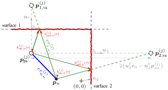
(a)

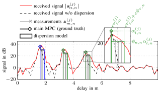
(b)

Figure 1: Exemplary indoor environment LABEL:sub@fig:fp and representative realization of a received signal LABEL:sub@fig:signal. The floor plan in LABEL:sub@fig:fp includes an agent at position $\bm{p}_{n}$ and a PA at position $\bm{p}^{(j)}_{\text{pa}}$ and two VAs at positions $\bm{p}^{(j)}_{l,\text{va}}$ for corresponding surfaces. The signal shown in LABEL:sub@fig:signal is received by PA at position $\bm{p}^{(j)}_{\text{pa}}$. Non-ideal antennas or reflective surfaces as indicated in LABEL:sub@fig:fp by generic impulse responses $h_{\text{ant},n}^{(j)}(\tau)$ and $h_{\text{surf},n}^{(j)}(\tau)$ lead to the received signal $\bm{\mathsfbr{s}}_{\text{rx},n}^{(j)}$ shown in LABEL:sub@fig:signal (c.f. received signal without dispersion). Resulting measurements (MPC parameter estimates) $\bm{z}^{(j)}_{m,n}$ are indicated in the received signal $\bm{\mathsfbr{s}}_{\text{rx},n}^{(j)}$ shown in LABEL:sub@fig:signal alongside the proposed dispersion model.

III Radio Signal Model

At each time $n$, the mobile agent transmits a signal $s(t)$ from a single antenna and each PA $j\in\{1,\hskip 0.85358pt\dots\hskip 0.85358pt,J\}$ acts as a receiver having a single antenna. The received complex baseband signal at the $j$th PA is sampled $N_{\text{s}}$ times with sampling frequency $f_{\text{s}}=1/T_{\text{s}}$ yielding an observation period of $T=N_{\text{s}}\,T_{\text{s}}$. By stacking the samples, we obtain the discrete-time received signal vector

$$\bm{\mathsfbr{s}}_{\text{rx},n}^{(j)}=\sum_{l=1}^{{L}_{n}^{(j)}}{\alpha}_{l,n}^{(j)}\Big{(}\bm{s}\big{(}{\tau}_{l,n}^{(j)}\big{)}+\sum_{i=1}^{S_{l}^{(j)}}\beta^{(j)}_{l,i,n}\bm{s}\big{(}{\tau}_{l,n}^{(j)}+\nu^{(j)}_{l,i,n}\big{)}\Big{)}+\bm{\mathsfbr{w}}_{n}^{(j)}$$ (6)

where $\bm{s}(\tau)\triangleq[s(-(N_{\text{s}}-1)/2\hskip 0.85358ptT_{\text{s}}-\tau)\,\,\,\cdots\,\,\,s((N_{\text{s}}-1)/2\hskip 0.85358ptT_{\text{s}}-\tau)]^{\text{T}}\in\mathbb{C}^{N_{\text{s}}\times 1}$ is the discrete-time transmit pulse. The first term contains the sum over the LOS component ($l=1$) and the ${L}_{n}^{(j)}-1$ specular MPCs (for $l\in\{2,\dots,L_{n}^{(j)}\}$) termed main components. The $l$th main-component is characterized by its complex amplitude ${\alpha}_{l,n}^{(j)}\in\mathbb{C}$ and its delays ${\tau}_{l,n}^{(j)}$. The second term contains the sum over $S_{l}^{(j)}$ additional sub-components characterized by complex amplitudes ${\alpha}_{l,n}^{(j)}\beta^{(j)}_{l,i,n}$ and by (relative) delays ${\tau}_{l,n}^{(j)}+\nu^{(j)}_{l,i,n}$, where $\nu^{(j)}_{l,i,n}$ is the excess delay and $\beta^{(j)}_{l,i,n}\in\mathbb{R}$ is a relative dampening variable. The delays $\tau_{l,n}^{(j)}$ are proportional to the distances (ranges) between the agent and either the $j$th PA (for $l\!=\!1$) or the corresponding VAs (for $l\in\{2,\dots,L_{n}^{(j)}\}$). That is $\tau_{1,n}^{(j)}=\big{\|}\bm{p}_{n}\!-\bm{p}_{\text{pa}}^{(j)}\big{\|}/c$ and $\tau_{l,n}^{(j)}=\big{\|}\bm{p}_{n}\!-\bm{p}_{l,\text{va}}^{(j)}\big{\|}/c$ for $l\in\{2,\dots,L_{n}^{(j)}\}$, where $c$ is the speed of light. The measurement noise vector $\bm{\mathsfbr{w}}_{n}^{(j)}\in\mathbb{C}^{N_{\text{s}}\times 1}$ is a zero-mean, circularly-symmetric complex Gaussian random vector with covariance matrix ${\sigma}^{(j)\hskip 0.85358pt2}\bm{I}_{N_{\text{s}}}$ and noise variance ${\sigma}^{(j)\hskip 0.85358pt2}={N}_{0}^{(j)}/T_{\text{s}}$. The component SNR of MPC $l$ is $\mathrm{SNR}^{(j)}_{l,n}=|{\alpha}^{(j)}_{l,n}|^{2}\|\bm{s}({\tau}_{l,n}^{(j)})\|^{2}/{\sigma}^{(j)\hskip 0.85358pt2}$. The component SNR of the sub-components is given as $\mathrm{SNR}^{(j)}_{l,i,n}=\beta^{(j)\,2}_{l,i,n}\mathrm{SNR}^{(j)}_{l,n}$. The corresponding normalized amplitude is ${u}^{(j)}_{l,n}\triangleq\mathrm{SNR}^{(j)\hskip 0.85358pt\frac{1}{2}}_{l,n}$ and ${u}^{(j)}_{l,i,n}\triangleq\mathrm{SNR}^{(j)\hskip 0.85358pt\frac{1}{2}}_{l,i,n}$, respectively. Details about the signal model given in (6) are provided in Appendix A.

III-A Signal Model Assumptions

To capture effects such as non-calibrated antennas [22, Section VII-C], the scattering from a user-body [36, 37], rural environments [38, 39] as well as non-ideal reflective surfaces [6], we introduce the dispersion parameters $\psi^{(j)}_{\tau,l,n}$ and $\psi_{\text{u},l,n}^{(j)}$. In this work, we assume the following restrictions to this model: (i) the additional sub-components with excess delays $\nu^{(j)}_{l,i,n}\in[0,\psi^{(j)}_{\tau,l,n}]$ after each MPC $l$ have the same support, i.e., $\psi^{(j)}_{\tau,l,n}\triangleq\psi_{\tau,n}$ and (ii) the corresponding dampening variables are constant $\beta^{(j)}_{l,i,n}\triangleq\psi^{(j)}_{\text{u},l,n}$ with the same value for each MPC $l$, i.e., $\psi^{(j)}_{\text{u},l,n}\triangleq\psi_{\text{u},n}$. This model can be applied to ultra-wideband systems with non-calibrated antennas [22, Section VII-C] that introduce delay dispersion or to environments containing moderate non-ideal reflective surfaces [6, 7] that are approximately similar in behavior and do not change significantly over the explored area. An exemplary signal as well as the dispersion model is shown in Fig. 1b.

III-B Parametric Channel Estimation

By applying at each time $n$, a channel estimation and detection algorithm (CEDA) [18, 19, 20, 21, 22, 23] to the observed discrete signal vector $\bm{s}_{\text{rx},n}^{(j)}$, one obtains, for each anchor $j$, a number of $M_{n}^{(j)}$ measurements denoted by ${\bm{z}^{(j)}_{m,n}}$ with $m\in{\cal{M}}_{n}^{(j)}\triangleq\{1,\,\dots\,,M_{n}^{(j)}\}$. Each $\bm{z}^{(j)}_{m,n}=[{z_{\tau}^{(j)}}_{m,n}\ {z_{\mathrm{u}}^{(j)}}_{m,n}]^{\text{T}}$ representing a potential MPC parameter estimate, contains a delay measurement ${z_{\tau}^{(j)}}_{m,n}\in[0,\tau_{\text{max}}]$ and a normalized amplitude measurement ${z_{\mathrm{u}}^{(j)}}_{m,n}\in[\gamma,\infty)$, where $\gamma$ is the detection threshold. The CEDA decomposes the signal $\bm{\mathsfbr{s}}_{\text{rx},n}^{(j)}$ into individual, decorrelated components according to (6), reducing the number of dimensions (as ${M}_{n}^{(j)}$ is usually much smaller than $N_{\text{s}}$). It thus compresses the information contained in $\bm{\mathsfbr{s}}_{\text{rx},n}^{(j)}$ into $\vspace*{-1mm}\bm{z}^{(j)}_{n}=[{\bm{z}^{(j)\text{T}}_{1,n}}\cdots{\bm{z}^{(j)\text{T}}_{M_{n}^{(j)},n}}]^{\text{T}}$. The stacked vector $\bm{z}_{n}=[\bm{z}^{(1)\,\text{T}}_{n}\cdots\bm{z}^{(J)\,\text{T}}_{n}]^{\text{T}}$ is used by the proposed algorithm as a noisy measurement.

IV System Model

At each time $n$, the state $\bm{\mathsfbr{x}}_{n}=[\bm{\mathsfbr{p}}_{n}^{\text{T}}\,\hskip 0.85358pt\bm{\mathsfbr{v}}_{n}^{\text{T}}]^{\text{T}}$ of the agent consists of its position $\bm{\mathsfbr{p}}_{n}$ and velocity $\bm{\mathsfbr{v}}_{n}$. We also introduce the augmented agent state $\tilde{\bm{\mathsfbr{x}}}_{n}=[\bm{\mathsfbr{x}}_{n}^{\text{T}}\,\hskip 0.85358pt\bm{\spsi}_{n}^{\text{T}}]^{\text{T}}$ that contains the dispersion parameters $\bm{\spsi}_{n}=[\spsi_{\tau,n}\hskip 2.84526pt\spsi_{\text{u},n}]^{\text{T}}$. In line with [26, 22, 11], we account for the unknown number of VAs by introducing for each PA $j$ potential s $k\in\mathcal{K}^{(j)}_{n}\triangleq\{1,\dots,{K}_{n}^{(j)}\}$. The number of PVAs $K_{n}^{(j)}$ is the maximum possible number of VAs of PA $j$ that produced measurements so far [26] (i.e., $K_{n}^{(j)}$ increases with time). The state of PVA $(j,k)$ is denoted as $\bm{\mathsfbr{y}}_{k,n}^{(j)}\!\triangleq\big{[}\bm{\mathsfbr{x}}_{k,n}^{(j)\text{T}}\,\hskip 0.85358pt\mathsfbr{r}_{k,n}^{(j)}\big{]}^{\text{T}}$ with $\bm{\mathsfbr{x}}_{k,n}^{(j)}=\big{[}\bm{\mathsfbr{p}}_{k,\text{va}}^{(j)\text{T}}\,\hskip 0.85358pt\mathsfbr{u}_{k,n}^{(j)}\big{]}^{\text{T}}$, which includes the normalized amplitude $\mathsfbr{u}_{k,n}^{(j)}$ [11, 22]. The existence/nonexistence of PVA $k$ is modeled by the existence variable $\mathsfbr{r}^{(j)}_{k,n}\in\{0,1\}$ in the sense that PVA $k$ exists if and only if $r^{(j)}_{k,n}\!=\!1$. The PVA state is considered formally also if PVA $k$ is nonexistent, i.e., if $r^{(j)}_{k,n}\!=0$.

Since a part of the PA state is unknown, we also consider the PA itself a PVA. Hence, we distinguish between the PVA $k=1$ that explicitly represents the PA, which is a-priori existent and has known and fixed position $\bm{p}_{1,\text{va}}^{(j)}=\bm{p}_{\text{pa}}^{(j)}$, and all other PVAs $k\in\{2,\hskip 0.85358pt\dots\hskip 0.85358pt,K_{n}^{(j)}\}$ whose existence and position are a-priori unknown. Note that the PVAs state representing the PA still considers the normalized amplitude $\mathsfbr{u}_{1,n}^{(j)}$ as well as the existence variable $\mathsfbr{r}^{(j)}_{1,n}$. The states $\bm{\mathsfbr{x}}^{(j)\hskip 0.85358pt\text{T}}_{k,n}$ of nonexistent PVAs are obviously irrelevant. Therefore, all PDFs defined for PVA states, $f(\bm{y}_{k,n})=f(\bm{x}_{k,n},r_{k,n})$, are of the form $f(\bm{x}^{(j)}_{k,n},0)$ $=f^{(j)}_{k,n}f_{\text{d}}(\bm{x}^{(j)}_{k,n})$, where $f_{\text{d}}(\bm{x}^{(j)}_{k,n})$ is an arbitrary “dummy” PDF and $f^{(j)}_{k,n}\!\in[0,1]$ is a constant. We also define the stacked vectors $\bm{\mathsfbr{y}}_{n}^{(j)}\!\triangleq\big{[}\bm{\mathsfbr{y}}_{1,n}^{(j)\text{T}}\cdots\hskip 0.85358pt\bm{\mathsfbr{y}}_{K_{n}^{(j)},n}^{(j)\text{T}}\big{]}^{\text{T}}$ and $\bm{\mathsfbr{y}}_{n}\!\triangleq\big{[}\bm{\mathsfbr{y}}_{n}^{(1)\text{T}}\cdots\hskip 0.85358pt\bm{\mathsfbr{y}}_{n}^{(J)\text{T}}\big{]}^{\text{T}}$. Note that according to the model introduced in Section III, $\bm{\spsi}_{n}$ is common for all PVAs. However, this model can be extended to individual dispersion parameters for each PVA (see [24]).

IV-A State Evolution

For each PVA with state $\bm{\mathsfbr{y}}_{k,n-1}^{(j)}$ with $k\in\mathcal{K}^{(j)}_{n-1}\triangleq\{1,\dots,{K}_{n-1}^{(j)}\}$ at time $n-1$ and PA $j$, there is one “legacy” PVA with state $\underline{\bm{\mathsfbr{y}}}_{k,n}^{(j)}\!\triangleq\big{[}\underline{\bm{\mathsfbr{x}}}_{k,n}^{(j)\text{T}}\,\hskip 0.85358pt\underline{\mathsfbr{r}}_{k,n}^{(j)}\big{]}^{\text{T}}$ with $k\in\mathcal{K}^{(j)}_{n-1}$ at time $n$ and PA $j$. We also define the joint states $\underline{\bm{\mathsfbr{y}}}_{n}^{(j)}\triangleq\big{[}\underline{\bm{\mathsfbr{y}}}_{1,n}^{(j)\text{T}}\cdots\hskip 0.85358pt\underline{\bm{\mathsfbr{y}}}_{K_{n-1}^{(j)},n}^{(j)\text{T}}\big{]}^{\text{T}}$ and $\underline{\bm{\mathsfbr{y}}}_{n}\!\triangleq\big{[}\underline{\bm{\mathsfbr{y}}}_{n}^{(1)\text{T}}\cdots\hskip 0.85358pt\underline{\bm{\mathsfbr{y}}}_{n}^{(J)\text{T}}\big{]}^{\text{T}}$. Assuming that the augmented agent state as well as the PVA states of all PAs evolve independently across $k$, $n$, and $j$, the joint state-transition PDF factorizes as [3, 26]

$$f\big{(}\tilde{\bm{x}}_{n},\underline{\bm{y}}_{n}|\tilde{\bm{x}}_{n-1},\bm{y}_{n-1}\big{)} =f(\bm{x}_{n}|\bm{x}_{n-1})f(\bm{\psi}_{n}|\bm{\psi}_{n-1})$$

$$\hskip 14.22636pt\times\prod_{j=1}^{J}\prod_{k=1}^{K_{n-1}^{(j)}}f\big{(}\underline{\bm{y}}_{k,n}^{(j)}\big{|}\bm{y}_{k,n-1}^{(j)}\big{)}$$ (7)

where $f(\underline{\bm{y}}_{k,n}^{(j)}|\bm{y}_{k,n-1}^{(j)})\triangleq f\big{(}\underline{\bm{x}}_{k,n}^{(j)},\underline{r}_{k,n}^{(j)}\big{|}\bm{x}_{k,n-1}^{(j)},r_{k,n-1}^{(j)}\big{)}\vspace*{0.5mm}$ is the legacy PVA state-transition PDF. If PVA did not exist at time $n-\!1$, i.e., $r_{k,n-1}^{(j)}\!=\!0$, it cannot exist as a legacy PVA at time $n$ either. Thus,

$$f\big{(} \underline{\bm{x}}_{k,n}^{(j)},r_{k,n}^{(j)}\big{|}\bm{x}_{k,n-1}^{(j)},0\big{)}=\begin{cases}f_{\text{d}}\big{(}\underline{\bm{x}}_{k,n}^{(j)}\big{)},&\!\!\!\underline{r}_{k,n}^{(j)}\!=0\\[0.0pt] 0,&\!\!\!\underline{r}_{k,n}^{(j)}\!=\!1.\end{cases}\!\!\!\!$$ (8)

If PVA existed at time $n-\!1$, i.e., $r_{k,n-1}^{(j)}\!=\!1$, it either dies, i.e., $\underline{r}_{k,n}^{(j)}\!=0$, or survives, i.e., $\underline{r}_{k,n}^{(j)}\!=\!1$ with survival probability denoted as $p_{\text{s}}$. If it does survive, its new state $\underline{\bm{\mathsfbr{y}}}_{k,n}^{(j)}$ is distributed according to the state-transition PDF $f\big{(}\underline{\bm{x}}_{k,n}^{(j)}\big{|}\bm{x}_{k,n-1}^{(j)}\big{)}\triangleq\delta\big{(}\underline{\bm{p}}_{k,\text{va}}^{(j)}-\bm{p}_{k,\text{va}}^{(j)}\big{)}f\big{(}u_{k,n}^{(j)}\big{|}u_{k,n-1}^{(j)}\big{)}$ [11, 3]. Thus,

$$f\big{(}\underline{\bm{x}}_{k,n}^{(j)},\underline{r}_{k,n}^{(j)}\big{|}\bm{x}_{k,n-1}^{(j)},1\big{)}$$

$$\hskip 11.38109pt=\begin{cases}(1\!-p_{\text{s}})\hskip 0.85358ptf_{\text{d}}\big{(}\underline{\bm{x}}_{k,n}^{(j)}\big{)},&\!\!\!\underline{r}_{k,n}^{(j)}\!=0\\[0.0pt] p_{\text{s}}\hskip 0.85358pt\delta\big{(}\underline{\bm{p}}_{k,\text{va}}^{(j)}-\bm{p}_{k,\text{va}}^{(j)}\big{)}f\big{(}u_{k,n}^{(j)}\big{|}u_{k,n-1}^{(j)}\big{)},&\!\!\!\underline{r}_{k,n}^{(j)}\!=\!1\end{cases}\hskip 0.85358pt.$$ (9)

The agent state $\bm{\mathsfbr{x}}_{n}$ with state-transition PDF $f(\bm{x}_{n}|\bm{x}_{n-1})$ is assumed to evolve in time according to a 2-dimensional, constant velocity and stochastic acceleration model [40] (linear movement) given as $\bm{\mathsfbr{x}}_{n}=\bm{A}\,\bm{\mathsfbr{x}}_{n-1}+\bm{B}\,\bm{\mathsfbr{w}}_{n}$, with the acceleration process $\bm{\mathsfbr{w}}_{n}$ being independent and identically distributed (iid) across $n$, zero mean, and Gaussian with covariance matrix ${\sigma_{\text{w}}^{2}}\,\bm{I}_{2}$, ${\sigma_{\text{w}}}$ is the acceleration standard deviation, and $\bm{A}\in\mathbb{R}^{4\times 4}$ and $\bm{B}\in\mathbb{R}^{4\times 2}$ are defined according to [40, p. 273], with observation period $\Delta T$. The state-transition PDFs of the dispersion parameter states $f(\bm{\psi}_{n}|\bm{\psi}_{n-1})=f({\psi}_{\tau,n}|\psi_{\tau,n-1})f(\psi_{\text{u},n}|\psi_{\text{u},n-1})$ are assumed to evolve independently of each other across $n$. Since both dispersion parameters are strictly positive and independent, we model the individual state-transition PDFs by Gamma PDFs given respectively by $f(\psi_{\tau,n}|\psi_{\tau,n-1})=\mathcal{G}(\psi_{\tau,n};q_{\tau},\psi_{\tau,n-1}/q_{\tau})$ and $f(\psi_{\text{u},n}|\psi_{\text{u},n-1})=\mathcal{G}(\psi_{\text{u},n};q_{\text{u}},\psi_{\text{u},n-1}/q_{\text{u}})$, where $q_{\tau}$ and $q_{\text{u}}$ represent the respective state noise parameters [27, 24]. Note that a small $q$ implies a large state transition uncertainty. The state-transition PDF of the normalized amplitude $\underline{u}_{k,n}^{(j)}$ is modeled by a truncated Rician PDF, i.e., $f(\underline{u}_{k,n}^{(j)}|u_{k,n-1}^{(j)})=f_{\text{TRice}}(\underline{u}_{k,n}^{(j)};\sigma_{\text{u},k},u^{(j)}_{k,n-1},0)$ with state noise parameter $\sigma_{\text{u},k}$. The truncated Rician PDF was found to be useful for the proposed amplitude model [22] (see (IV-B) in Section IV-B).

IV-B Measurement Model

At each time $n$ and for each anchor $j$, the CEDA provides the currently observed measurement vector $\bm{z}_{n}^{(j)}$, with fixed ${M}^{(j)}_{n}$, according to Section III-B. Before the measurements are observed, they are random and represented by the vector ${\bm{\mathsfbr{z}}^{(j)}_{m,n}}=[{\mathsfbr{z}_{\tau}^{(j)}}_{m,n}~{}{\mathsfbr{z}_{\mathrm{u}}^{(j)}}_{m,n}]^{\text{T}}$. In line with Section III-B we define the nested random vectors $\bm{\mathsfbr{z}}^{(j)}_{n}=[{\bm{\mathsfbr{z}}^{(j)\text{T}}_{1,n}}\cdots\hskip 0.85358pt{\bm{\mathsfbr{z}}^{(j)\text{T}}_{\mathsfbr{M}_{n}^{(j)},n}}]^{\text{T}}$, with length corresponding to the random number of measurements $\mathsfbr{M}^{(j)}_{n}$, and $\bm{\mathsfbr{z}}_{n}=[\bm{\mathsfbr{z}}^{(1)\,\text{T}}_{n}\cdots\hskip 0.85358pt\bm{\mathsfbr{z}}^{(J)\,\text{T}}_{n}]^{\text{T}}$. The vector containing all numbers of measurements is defined as $\bm{\mathsfbr{M}}_{n}=[\mathsfbr{M}_{n}^{(1)}\hskip 0.85358pt\cdots\hskip 0.85358pt\mathsfbr{M}_{n}^{(J)}]^{\text{T}}$.

If PVA $k$ exists ($r^{(j)}_{k,n}=1$), it gives rise to a random number of measurements. The mean number of measurements per (existing) PVA is modeled by a Poisson point process with mean $\mu_{\text{m}}\big{(}{\bm{\psi}}_{n},{u}^{(j)}_{k,n}\big{)}$. The individual measurements $\bm{\mathsfbr{z}}^{(j)}_{m,n}$ are assumed to be conditionally independent, i.e., the joint PDF of all measurements factorizes as $f(\bm{z}_{n}^{(j)}|{M}_{n}^{(j)},{\bm{x}}_{n},{\nu}_{k,n}^{(j)},{\beta}_{k,n}^{(j)},\bm{x}_{k,n}^{(j)})=\prod_{m=1}^{{M}_{n}^{(j)}}f(\bm{z}_{m,n}^{(j)}|{\bm{x}}_{n},{\nu}_{k,n}^{(j)},{\beta}_{k,n}^{(j)},\bm{x}_{k,n}^{(j)})$.

If ${\bm{\mathsfbr{z}}^{(j)}_{m,n}}$ is generated by a PVA, i.e., it corresponds to a main-component (LOS component or MPC), we assume that the single-measurement likelihood function $f(\bm{z}_{m,n}^{(j)}|{\bm{x}}_{n},{\nu}_{k,n}^{(j)},{\beta}_{k,n}^{(j)},\bm{x}_{k,n}^{(j)})$ is conditionally independent across ${\mathsfbr{z}_{\tau}^{(j)}}_{m,n}$ and ${\mathsfbr{z}_{\mathrm{u}}^{(j)}}_{m,n}$. Thus, it factorizes as

$$f(\bm{z}_{m,n}^{(j)}|{\bm{x}}_{n},{\nu}_{k,n}^{(j)},{\beta}_{k,n}^{(j)},\bm{x}_{k,n}^{(j)})$$

$$\hskip 5.69054pt=f({z_{\tau}^{(j)}}_{m,n}|\bm{p}_{n},{\nu}_{k,n}^{(j)},{\beta}_{k,n}^{(j)},\bm{x}_{k,n}^{(j)})f({z_{\mathrm{u}}^{(j)}}_{m,n}|{\beta}_{k,n}^{(j)},{u}_{k,n}^{(j)}).$$ (10)

The likelihood function of the corresponding delay measurement ${\mathsfbr{z}_{\tau}^{(j)}}_{m,n}$ is given by

$$f({z_{\tau}^{(j)}}_{m,n}|\bm{p}_{n},{\nu}_{k,n}^{(j)},{\beta}_{k,n}^{(j)},\bm{x}_{k,n}^{(j)})$$

$$\hskip 14.22636pt=f_{\text{N}}\Big{(}{z_{\tau}^{(j)}}_{m,n};\,\tau(\bm{p}_{k,\text{va}}^{(j)},\bm{p}_{n})+\nu_{k,n}^{(j)},\,\sigma_{\tau}^{2}({\beta}_{k,n}^{(j)}u_{k,n}^{(j)})\Big{)}$$ (11)

with mean $\tau(\bm{\mathsfbr{p}}_{k,\text{va}}^{(j)},\bm{\mathsfbr{p}}_{n})+\snu_{k,n}^{(j)}$ and variance $\sigma_{\tau}^{2}(\sbeta_{k,n}^{(j)}\mathsfbr{u}_{k,n}^{(j)})$ where $\tau(\bm{\mathsfbr{p}}_{k,\text{va}}^{(j)},\bm{\mathsfbr{p}}_{n})=\lVert\bm{\mathsfbr{p}}_{n}-\bm{\mathsfbr{p}}_{k,\text{va}}^{(j)}\rVert/c$. The standard deviation is determined from the Fisher information given by $\sigma_{\tau}^{2}(u)=c^{2}/(8\,\pi^{2}\,\beta_{\text{bw}}^{2}\,u^{2})$ with $\beta_{\text{bw}}$ being the root mean squared bandwidth [42, 43] (see Section VI). The likelihood function of the corresponding normalized amplitude measurement ${z_{\mathrm{u}}^{(j)}}_{m,n}$ is obtained as

$$f({z_{\mathrm{u}}^{(j)}}_{m,n}|{\beta}_{k,n}^{(j)},u_{k,n}^{(j)})$$

$$\hskip 22.76219pt\triangleq f_{\text{TRice}}({z_{\mathrm{u}}^{(j)}}_{m,n};\sigma_{\mathrm{u}}({\beta}_{k,n}^{(j)}u_{k,n}^{(j)}),{\beta}_{k,n}^{(j)}u_{k,n}^{(j)},\gamma)$$ (12)

with scale parameter $\sigma_{\mathrm{u}}(\sbeta_{k,n}^{(j)}\mathsfbr{u}_{k,n}^{(j)})$, non-centrality parameter $\sbeta_{k,n}^{(j)}\mathsfbr{u}_{k,n}^{(j)}$, and detection threshold $\gamma$ [22, 46]. The scale parameter is similarly determined from the Fisher information given by

$$\sigma_{\mathrm{u}}^{2}(u)=1/2+u\,/(4N_{\text{s}})\hskip 0.85358pt.$$ (13)

Note that this expression reduces to $1/2$ if the additive white Gaussian noise (AWGN) noise variance $\sigma^{(j)\hskip 0.5pt2}$ is assumed to be known or $N_{\text{s}}$ to grow indefinitely (see [22, Appendix D] for a detailed derivation). The probability of detection resulting from (IV-B) is given by the Marcum Q-function, i.e., $p_{\text{D}}(\sbeta_{k,n}^{(j)}\mathsfbr{u}_{k,n}^{(j)})\triangleq Q_{1}(u/{\sigma_{\mathrm{u}}({\beta}_{k,n}^{(j)}u_{k,n}^{(j)})},{\gamma}/{\sigma_{\mathrm{u}}({\beta}_{k,n}^{(j)}u_{k,n}^{(j)})})$ [47, 22] (see Section I-C). Using the assumptions introduced in the Section III-A, the joint PDF of the dispersion variables can be constructed as follows

$$f(\nu_{k,n}^{(j)},{\beta}_{k,n}^{(j)}|\bm{\psi}_{n})= \frac{1}{2}\left(\delta(\nu_{k,n}^{(j)})\,\delta({\beta}_{k,n}^{(j)}-1)\right.$$

$$+\left.f_{\text{U}}(\nu_{k,n}^{(j)};0,{\psi}_{\tau,n})\delta({\beta}_{k,n}^{(j)}-{\psi}_{\text{u},n})\right)$$ (14)

where the according delay dispersion random variable is given as $\snu_{k,n}^{(j)}\sim f_{\text{U}}({\nu}_{k,n}^{(j)};0,{\psi}_{\tau,n})$ and the amplitude dispersion random variable is $\sbeta_{k,n}^{(j)}\sim\delta({\beta}_{k,n}^{(j)}-{\psi}_{\text{u},n})$. The PDF of a single measurement $\bm{\mathsfbr{z}}_{m,n}^{(j)}$ can now be obtained by integrating out the dispersion variables as

$$f(\bm{z}_{m,n}^{(j)}|\tilde{\bm{x}}_{n},\bm{x}_{k,n}^{(j)})=f(\bm{z}_{m,n}^{(j)}|{\bm{x}}_{n},\bm{\psi}_{n},\bm{x}_{k,n}^{(j)})$$

$$=\int f(\bm{z}_{m,n}^{(j)}|{\bm{x}}_{n},{\nu}_{k,n}^{(j)},{\beta}_{k,n}^{(j)},\bm{x}_{k,n}^{(j)})$$

$$\hskip 42.67912pt\times f(\nu_{k,n}^{(j)},{\beta}_{k,n}^{(j)}|\bm{\psi}_{n})\mathrm{d}\nu_{k,n}^{(j)}\,\mathrm{d}{\beta}_{k,n}^{(j)}$$

$$=f({z_{\tau}^{(j)}}_{m,n}|\bm{p}_{n},\bm{x}_{k,n}^{(j)})f({z_{\mathrm{u}}^{(j)}}_{m,n}|u_{k,n}^{(j)})$$

$$\hskip 28.45274pt+f({z_{\tau}^{(j)}}_{m,n}|\bm{p}_{n},\bm{\psi}_{n},\bm{x}_{k,n}^{(j)})f({z_{\mathrm{u}}^{(j)}}_{m,n}|u_{k,n}^{(j)},\psi_{\text{u},n})$$ (15)

with the main-component delay PDF

$$f({z_{\tau}^{(j)}}_{m,n}|\bm{p}_{n},\bm{x}_{k,n}^{(j)})=f_{\text{N}}({z_{\tau}^{(j)}}_{m,n};\,\tau(\bm{p}_{k,\text{va}}^{(j)},\bm{p}_{n}),\,\sigma_{\tau}^{2}(u_{k,n}^{(j)}))$$ (16)

and the main-component amplitude PDF

$$f({z_{\mathrm{u}}^{(j)}}_{m,n}|u_{k,n}^{(j)})=f_{\text{TRice}}({z_{\mathrm{u}}^{(j)}}_{m,n};\sigma_{\mathrm{u}}(u_{k,n}^{(j)}),u_{k,n}^{(j)},\gamma)$$ (17)

as well as the additional sub-component delay PDF

$$f({z_{\tau}^{(j)}}_{m,n}|\bm{p}_{n},\bm{\psi}_{n},\bm{x}_{k,n}^{(j)})$$

$$=\frac{1}{{\psi}_{\tau,n}}\int_{0}^{{\psi}_{\tau,n}}f_{\text{N}}\Big{(}{z_{\tau}^{(j)}}_{m,n};\tau(\bm{p}_{k,\text{va}}^{(j)},\bm{p}_{n})+\nu_{k,n}^{(j)},\sigma_{\tau}^{2}({\psi}_{\text{u},n}u_{k,n}^{(j)})\Big{)}\hskip 0.5pt\mathrm{d}\nu_{k,n}^{(j)}$$

$$=\frac{1}{2{\psi}_{\tau,n}}\Bigg{(}\text{erf}\left(\frac{\tau(\bm{p}_{k,\text{va}}^{(j)},\bm{p}_{n})+{\psi}_{\tau,n}-{z_{\tau}^{(j)}}_{m,n}}{\sigma_{\tau}({\psi}_{\text{u},n}u_{k,n}^{(j)})\sqrt{2}}\right)$$

$$\hskip 71.13188pt-\text{erf}\Bigg{(}\frac{\tau(\bm{p}_{k,\text{va}}^{(j)},\bm{p}_{n})-{z_{\tau}^{(j)}}_{m,n}}{\sigma_{\tau}({\psi}_{\text{u},n}u_{k,n}^{(j)})\sqrt{2}}\Bigg{)}\Bigg{)}$$ (18)

and the additional sub-component amplitude PDF

$$f({z_{\mathrm{u}}^{(j)}}_{m,n}|{\psi}_{\text{u},n},u_{k,n}^{(j)})$$

$$\hskip 28.45274pt=f_{\text{TRice}}({z_{\mathrm{u}}^{(j)}}_{m,n};\sigma_{\mathrm{u}}({\psi}_{\text{u},n}u_{k,n}^{(j)}),{\psi}_{\text{u},n}u_{k,n}^{(j)},\gamma).$$ (19)

The according probability of detection is given as $p_{\text{D}}(\mathsfbr{u}_{k,n}^{(j)})$ for the main-component of each PVA or $p_{\text{D}}(\spsi_{\text{u},n}\mathsfbr{u}_{k,n}^{(j)})$ for the additional sub-components, respectively.

It is also possible that a measurement $\bm{\mathsfbr{z}}_{m,n}^{(j)}$ did not originate from any PVA (false alarm). False alarm measurements originating from the CEDA are assumed statistically independent of PVA states. They are modeled by a Poisson point process with mean ${{\mu}_{\mathrm{fa}}}$ and PDF $f_{\mathrm{fa}}(\bm{z}_{m,n}^{(j)})$, which is assumed to factorize as $f_{\mathrm{fa}}(\bm{z}_{m,n}^{(j)})={f_{\mathrm{fa}}}({z_{\tau}^{(j)}}_{m,n}){f_{\mathrm{fa}}}({z_{\mathrm{u}}}_{m,n}^{(j)})$. The false alarm PDF for a single delay measurement is assumed to be uniformly distributed as ${f_{\mathrm{fa}}}({z_{\tau}^{(j)}}_{m,n})=f_{\mathrm{U}}({z_{\tau}^{(j)}}_{m,n};0,\tau_{\text{max}})$. In correspondence to (IV-B) the false alarm likelihood function of the normalized amplitude measurement is given as $f_{\mathrm{fa}}({z_{\mathrm{u}}^{(j)}}_{m,n})\triangleq f_{\text{TRayl}}({z_{\mathrm{u}}^{(j)}}_{m,n}\,;\sqrt{1/2}\,,\gamma)$ with the scale parameter given as $\sqrt{1/2}$ and detection threshold $\gamma$.

Considering the measurement model for the normalized amplitudes in (IV-B), the mean number of PVA-related measurements $\mu_{\text{m}}\big{(}\tilde{\bm{\mathsfbr{x}}}_{n},\bm{\mathsfbr{x}}^{(j)}_{k,n}\big{)}\triangleq\mu_{\text{m}}\big{(}{\bm{\spsi}}_{n},\mathsfbr{u}^{(j)}_{k,n}\big{)}$ is well approximated as

$$\mu_{\text{m}}\big{(}{\bm{\spsi}}_{n},\mathsfbr{u}^{(j)}_{k,n}\big{)}=p_{\text{D}}(\mathsfbr{u}_{k,n}^{(j)})+\frac{N_{\text{ny}}\,\spsi_{\tau,n}}{c\,{T}_{\text{s}}}\,p_{\text{D}}(\spsi_{\text{u},n}\mathsfbr{u}_{k,n}^{(j)})\hskip 0.85358pt.$$ (20)

The right-hand side fraction denotes the average number of additional sub-components estimated by the CEDA at a detection threshold of $\gamma=0~{}\mathrm{dB}$, where we assume an average of $N_{\text{ny}}$ components to be detected within one Nyquist sample. Accordingly, the mean number of false alarms is approximated as $\mu_{\text{fa}}=N_{\text{ny}}\hskip 0.5ptN_{\text{s}}\,e^{-\gamma^{2}}$ with $e^{-\gamma^{2}}=\int_{\gamma}^{\infty}f_{\mathrm{fa}}({z_{\mathrm{u}}^{(j)}}_{m,n})\,\mathrm{d}{z_{\mathrm{u}}^{(j)}}_{m,n}$ denoting the false alarm probability.

IV-C New PVAs

Newly detected PVAs, i.e., actual VAs that generate a measurement for the first time, are modeled by a Poisson point process with mean $\mu_{\text{n}}$ and PDF $f_{\text{n}}\big{(}\overline{\bm{x}}^{(j)}_{m,n}|\tilde{\bm{x}}_{n}\big{)}$. Following [3, 26], newly detected VAs are represented by new PVA states $\overline{\bm{\mathsfbr{y}}}^{(j)}_{m,n}$, $m\in\{1,\dots,M_{n}^{(j)}\}$, where each new PVA state corresponds to a measurement $\bm{\mathsfbr{z}}_{m,n}^{(j)}$; $\overline{r}_{m,n}^{(j)}=1$ implies that measurement $\bm{\mathsfbr{z}}_{m,n}^{(j)}$ was generated by a newly detected VA. Since newly detected VAs can potentially produce more than one measurement, we use the multiple-measurement-to-feature probabilistic data association and define this mapping as introduced in [24, 29]. We also introduce the joint states $\overline{\bm{\mathsfbr{y}}}_{n}^{(j)}\!\triangleq\big{[}\overline{\bm{\mathsfbr{y}}}_{1,n}^{(j)\text{T}}\cdots\hskip 0.85358pt\overline{\bm{\mathsfbr{y}}}_{M_{n}^{(j)},n}^{(j)\text{T}}\big{]}^{\text{T}}$ and $\overline{\bm{\mathsfbr{y}}}_{n}\!\triangleq\big{[}\overline{\bm{\mathsfbr{y}}}_{n}^{(1)\text{T}}\cdots\hskip 0.85358pt\overline{\bm{\mathsfbr{y}}}_{n}^{(J)\text{T}}\big{]}^{\text{T}}$. The vector of all PVAs at time $n$ is given by $\bm{\mathsfbr{y}}_{n}\!\triangleq\big{[}\underline{\bm{\mathsfbr{y}}}_{n}^{\text{T}}\,\hskip 0.85358pt\overline{\bm{\mathsfbr{y}}}_{n}^{\text{T}}\big{]}^{\text{T}}$. Note that the total number of PVAs per PA is given by $K_{n}^{(j)}=K_{n-1}^{(j)}+M_{n}^{(j)}$.

Since new PVAs are introduced as new measurements are available at each time, the number of PVAs grows indefinitely. Thus, for feasible methods a suboptimal pruning step is employed that removes unlikely PVAs (see Section IV-F).

IV-D Association Vectors

For each PA, measurements $\bm{z}_{m,n}^{(j)}$ are subject to a data association uncertainty. It is not known which measurement $\bm{z}_{m,n}^{(j)}$ is associated with which PVA $k$, or if a measurement $\bm{z}_{m,n}^{(j)}$ did not originate from any PVA (false alarm) or if a PVA did not give rise to any measurement (missed detection). The associations between measurements $\bm{z}_{m,n}^{(j)}$ and the PVAs at time $n$ is described by the binary PVA-orientated association variables with entries [29, 24]

$$\mathsfbr{a}_{km,n}^{(j)}\triangleq\begin{cases}1,&\!\begin{minipage}[t]{184.9429pt}if measurement $m$ was generated by \acs{pva} $k$\end{minipage}\\ 0\hskip 0.85358pt,&\!\begin{minipage}[t]{184.9429pt} otherwise\hskip 0.85358pt.\end{minipage}\end{cases}$$

We distinguish between legacy and new PVA-associated variable vectors given, respectively, as $\underline{\bm{\mathsfbr{a}}}_{k,n}^{(j)}\triangleq[\underline{\mathsfbr{a}}_{k1,n}^{(j)}\hskip 2.84526pt\cdots\hskip 2.84526pt\underline{\mathsfbr{a}}_{kM_{n}^{(j)},n}^{(j)}]^{\text{T}}$ with $k\in\mathcal{K}_{n-1}^{(j)}$ and $\overline{\bm{\mathsfbr{a}}}_{k,n}^{(j)}\triangleq[\overline{\mathsfbr{a}}_{k1,n}^{(j)}$ $\cdots\hskip 2.84526pt\overline{\mathsfbr{a}}_{kk,n}^{(j)}]^{\text{T}}$ with $k\in\mathcal{M}_{n}^{(j)}$ and $\bm{\mathsfbr{a}}_{k,n}^{(j)}\triangleq[\underline{\bm{\mathsfbr{a}}}_{k,n}^{(j)\text{T}}\hskip 2.84526pt\cdots\hskip 2.84526pt\overline{\bm{\mathsfbr{a}}}_{k,n}^{(j)\text{T}}]^{\text{T}}$ [29]. We also define $\bm{\mathsfbr{a}}_{n}^{(j)}\triangleq[\bm{\mathsfbr{a}}_{1,n}^{(j)\text{T}}\hskip 2.84526pt\cdots\hskip 2.84526pt\bm{\mathsfbr{a}}_{K_{n}^{(j)},n}^{(j)\text{T}}]^{\text{T}}$ and $\bm{\mathsfbr{a}}_{n}\triangleq[\bm{\mathsfbr{a}}_{n}^{(1)\text{T}}\hskip 2.84526pt\cdots\hskip 2.84526pt\bm{\mathsfbr{a}}_{n}^{(J)\text{T}}]^{\text{T}}\vspace*{0.2mm}$. To reduce computational complexity, following [25, 26, 3], we use the redundant description of association variables, i.e., we introduce measurement-orientated association variable

$$\mathsfbr{b}_{m,n}^{(j)}\triangleq\begin{cases}k\in\{1,\dots,K_{n}^{(j)}\},&\!\begin{minipage}[t]{128.0374pt}if measurement $m$ was \\ generated by \acs{pva} $k$\end{minipage}\\ 0\hskip 0.85358pt,&\!\begin{minipage}[t]{128.0374pt} otherwise \end{minipage}\end{cases}$$

and define the measurement-oriented association vector $\bm{\mathsfbr{b}}^{(j)}_{n}=[\mathsfbr{b}_{1,n}^{(j)}\hskip 2.84526pt\cdots\hskip 2.84526pt\mathsfbr{b}_{M_{n}^{(j)},n}^{(j)}]$. We also define $\bm{\mathsfbr{b}}_{n}\triangleq[\bm{\mathsfbr{b}}_{n}^{(1)\text{T}}\hskip 2.84526pt\cdots\hskip 2.84526pt\bm{\mathsfbr{b}}_{n}^{(J)\text{T}}]^{\text{T}}$. Note that any data association event that can be expressed by both random vectors $\bm{\mathsfbr{a}}_{n}$ and $\bm{\mathsfbr{b}}_{n}$ is a valid event, i.e., any measurement can be generated by at most one PVA. This redundant representation of events makes it possible to develop scalable SPAs [25, 26, 3, 22].

IV-E Joint Posterior PDF

By using common assumptions [26, 3, 22], and for fixed and thus observed measurements $\bm{z}_{1:n}$, it can be shown that the joint posterior PDF of $\tilde{\bm{\mathsfbr{x}}}_{1:n}$ ($\tilde{\bm{\mathsfbr{x}}}_{1:n}\triangleq[\tilde{\bm{\mathsfbr{x}}}_{1}^{\text{T}}\cdots\tilde{\bm{\mathsfbr{x}}}_{n}^{\text{T}}]^{\text{T}}$), $\bm{\mathsfbr{y}}_{1:n}$, $\bm{\mathsfbr{a}}_{1:n}$, and $\bm{\mathsfbr{b}}_{1:n}$, conditioned on $\bm{z}_{1:n}$ for all time steps $n^{\prime}\in\{1,\hskip 0.85358pt\dots\hskip 0.85358pt,n\}$ is given by

$$f(\tilde{\bm{x}}_{1:n},\bm{y}_{1:n},\bm{a}_{1:n},\bm{b}_{1:n}|\bm{z}_{1:n})$$

$$\propto f(\bm{x}_{1})f(\bm{\psi}_{1})\Bigg{(}\prod^{J}_{j^{\prime}=1}\prod^{K^{(j^{\prime})}_{1}}_{k^{\prime}=1}\!f\big{(}\underline{\bm{y}}^{(j^{\prime})}_{k^{\prime}\!,1}\big{)}\Bigg{)}$$

$$\times\ \prod^{n}_{n^{\prime}=2}\!f(\bm{x}_{n^{\prime}}|\bm{x}_{n^{\prime}-1})f(\bm{\psi}_{n^{\prime}}|\bm{\psi}_{n^{\prime}-1})$$

$$\times\ \prod^{J}_{j=1}\Bigg{(}\prod^{K^{(j)}_{n^{\prime}-1}}_{k=1}g\big{(}\underline{\bm{y}}^{(j)}_{k,n^{\prime}}\big{|}\bm{y}^{(j)}_{k,n^{\prime}-1},\tilde{\bm{x}}_{n^{\prime}-1}\big{)}$$

$$\times\prod^{M^{(j)}_{n^{\prime}}}_{m^{\prime}=1}q\big{(}\tilde{\bm{x}}_{n^{\prime}},\underline{\bm{y}}^{(j)}_{k,n^{\prime}},\underline{a}^{(j)}_{km^{\prime},n^{\prime}};\bm{z}^{(j)}_{m^{\prime},n^{\prime}}\big{)}\underline{\Psi}\big{(}\underline{a}^{(j)}_{km^{\prime},n^{\prime}},b^{(j)}_{m^{\prime},n^{\prime}}\big{)}\Bigg{)}$$

$$\times\Bigg{(}\prod^{M^{(j)}_{n^{\prime}}}_{m=1}v\big{(}\tilde{\bm{x}}_{n^{\prime}},\overline{\bm{y}}^{(j)}_{m,n^{\prime}},\overline{a}^{(j)}_{mm,n^{\prime}};\bm{z}^{(j)}_{m,n^{\prime}}\big{)}$$

$$\times\prod^{m-1}_{h=1}u\big{(}\tilde{\bm{x}}_{n^{\prime}},\overline{\bm{y}}^{(j)}_{m,n^{\prime}},\overline{a}^{(j)}_{mh,n^{\prime}};\bm{z}^{(j)}_{h,n^{\prime}}\big{)}\overline{\Psi}(\overline{a}^{(j)}_{mh,n^{\prime}},b^{(j)}_{h,n^{\prime}})\Bigg{)}$$ (21)

where $g(\underline{\bm{y}}^{(j)}_{k,n}|\underline{\bm{y}}^{(j)}_{k,n-1},\tilde{\bm{x}}_{n-1})$, $q\big{(}\tilde{\bm{x}}_{n},\underline{\bm{y}}^{(j)}_{k,n},\underline{a}^{(j)}_{km,n};\bm{z}^{(j)}_{m,n}\big{)}$, $\Psi(a^{(j)}_{km,n},b^{(j)}_{m,n})$, $u\big{(}\tilde{\bm{x}}_{n},\overline{\bm{y}}^{(j)}_{k,n},\overline{a}^{(j)}_{mh,n};\bm{z}^{(j)}_{h,n}\big{)}$ and $v\big{(}\tilde{\bm{x}}_{n},\overline{\bm{y}}^{(j)}_{m,n},\overline{a}^{(j)}_{mm,n};\bm{z}^{(j)}_{m,n}\big{)}$ are explained in what follows. The pseudo state-transition function is given by

$$g(\underline{\bm{y}}^{(j)}_{k,n}|\underline{\bm{y}}^{(j)}_{k,n-1},\tilde{\bm{x}}_{n-1})$$

$$\triangleq\begin{cases}e^{-\mu_{\text{m}}\big{(}\tilde{\bm{x}}_{n-1},\underline{\bm{x}}^{(j)}_{k,n}\big{)}}f(\underline{\bm{x}}^{(j)}_{k,n},1|\underline{\bm{x}}^{(j)}_{k,n-1},\underline{r}^{(j)}_{k,n-1}),&\underline{r}^{(j)}_{k,n}=1\\[2.84526pt] f(\underline{\bm{x}}^{(j)}_{k,n},0|\underline{\bm{x}}^{(j)}_{k,n-1},\underline{r}^{(j)}_{k,n-1}),&\underline{r}^{(j)}_{k,n}=0\end{cases}$$ (22)

and the pseudo prior distribution as

$$f(\overline{\bm{y}}^{(j)}_{k,n}|\tilde{\bm{x}}_{n})\triangleq\begin{cases}\mu_{n}f_{n}\big{(}\overline{\bm{x}}^{(j)}_{k,n}|\tilde{\bm{x}}_{n}\big{)}e^{-\mu_{\text{m}}\big{(}\tilde{\bm{x}}_{n},\overline{\bm{x}}^{(j)}_{k,n}\big{)}},&\overline{r}^{(j)}_{k,n}=1\\[2.84526pt] f_{d}\big{(}\overline{\bm{x}}^{(j)}_{k,n}\big{)},&\overline{r}^{(j)}_{k,n}=0\hskip 0.85358pt.\end{cases}$$ (23)

The pseudo likelihood functions related to legacy PVAs for $k\in{\cal{K}}_{n-1}^{(j)}$ $q\big{(}\tilde{\bm{x}}_{n},\underline{\bm{y}}^{(j)}_{k,n},\underline{a}^{(j)}_{km,n};\bm{z}^{(j)}_{m,n}\big{)}=q\big{(}\tilde{\bm{x}}_{n},\underline{\bm{x}}^{(j)}_{k,n},\underline{r}^{(j)}_{k},\underline{a}^{(j)}_{km,n};\bm{z}^{(j)}_{m,n}\big{)}$ is given by

$$q\big{(}\tilde{\bm{x}}_{n},\underline{\bm{x}}^{(j)}_{k,n},1,\underline{a}^{(j)}_{km,n};\bm{z}^{(j)}_{m,n}\big{)}$$

$$\hskip 14.22636pt\triangleq\begin{cases}\frac{\mu_{\text{m}}\big{(}\tilde{\bm{x}}_{n},\underline{\bm{x}}^{(j)}_{k,n}\big{)}f(\bm{z}^{(j)}_{m,n}|\bm{p}_{n},\bm{\psi}_{n},\underline{\bm{x}}_{k,n}^{(j)})}{\mu_{\text{fa}}f_{\text{fa}}(\bm{z}^{(j)}_{m,n})},&\underline{a}^{(j)}_{km,n}=1\\ 1,&\underline{a}^{(j)}_{km,n}=0\\ \end{cases}$$ (24)

and $q\big{(}\tilde{\bm{x}}_{n},\underline{\bm{x}}^{(j)}_{k,n},0,\underline{a}^{(j)}_{km,n};\bm{z}^{(j)}_{m,n}\big{)}\triangleq\delta_{\underline{a}^{(j)}_{km,n}}$. The pseudo likelihood functions related to a new PVA (with $k\in{\cal{M}}_{n}^{(j)}\backslash m$) is given as $u\big{(}\tilde{\bm{x}}_{n},\overline{\bm{y}}^{(j)}_{k,n},\overline{a}^{(j)}_{km,n};\bm{z}^{(j)}_{m,n}\big{)}=u\big{(}\tilde{\bm{x}}_{n},\overline{\bm{x}}^{(j)}_{k,n},\overline{r}^{(j)}_{k},\overline{a}^{(j)}_{km,n};\bm{z}^{(j)}_{m,n}\big{)}$ is given by

$$u\big{(}\tilde{\bm{x}}_{n},\overline{\bm{x}}^{(j)}_{k,n},1,\overline{a}^{(j)}_{km,n};\bm{z}^{(j)}_{m,n}\big{)}$$

$$\hskip 5.69054pt\triangleq\begin{cases}\frac{f(\overline{\bm{y}}^{(j)}_{k,n}|\tilde{\bm{x}}_{n})\mu_{\text{m}}\big{(}\tilde{\bm{x}}_{n},\overline{\bm{x}}^{(j)}_{k,n}\big{)}f(\bm{z}^{(j)}_{m,n}|\bm{p}_{n},\bm{\psi}_{n},\overline{\bm{x}}_{k,n}^{(j)})}{\mu_{\text{fa}}f_{\text{fa}}(\bm{z}^{(j)}_{m,n})},&\overline{a}^{(j)}_{km,n}=1\\ 1,&\overline{a}^{(j)}_{km,n}=0\\ \end{cases}$$ (25)

and $u\big{(}\tilde{\bm{x}}_{n},\overline{\bm{x}}^{(j)}_{k,n},0,\overline{a}^{(j)}_{km,n};\bm{z}^{(j)}_{m,n}\big{)}\triangleq\delta_{\overline{a}^{(j)}_{km,n}}$, whereas for $k=m$ as $v\big{(}\tilde{\bm{x}}_{n},\overline{\bm{y}}^{(j)}_{m},\overline{a}^{(j)}_{mm,n};\bm{z}^{(j)}_{m,n}\big{)}=v\big{(}\tilde{\bm{x}}_{n},\overline{\bm{x}}^{(j)}_{m,n},\overline{r}^{(j)}_{m,n},\overline{a}^{(j)}_{mm,n};\bm{z}^{(j)}_{m,n}\big{)}$ is given by

$$v\big{(}\tilde{\bm{x}}_{n},\overline{\bm{x}}^{(j)}_{m,n},1,\overline{a}^{(j)}_{mm,n};\bm{z}^{(j)}_{m,n}\big{)}$$

$$\hskip 2.84526pt\triangleq\begin{cases}\frac{f(\overline{\bm{y}}^{(j)}_{m,n}|\tilde{\bm{x}}_{n})\mu_{\text{m}}\big{(}\tilde{\bm{x}}_{n},\overline{\bm{x}}^{(j)}_{m,n}\big{)}f\big{(}\bm{z}^{(j)}_{m,n}|\bm{p}_{n},\bm{\psi}_{n},\overline{\bm{x}}_{m,n}^{(j)}\big{)}}{\mu_{\text{fa}}f_{\text{fa}}(\bm{z}^{(j)}_{m,n})},&\overline{a}^{(j)}_{mm,n}=1\\ 0,&\overline{a}^{(j)}_{mm,n}=0\\ \end{cases}$$ (26)

and $v\big{(}\tilde{\bm{x}}_{n},\overline{\bm{x}}^{(j)}_{m,n},0,\overline{a}^{(j)}_{mm,n};\bm{z}^{(j)}_{m,n}\big{)}\triangleq\delta_{\overline{a}^{(j)}_{mm,n}}$.

Finally, the binary indicator functions that check consistency for any pair $(a^{(j)}_{km,n},b^{(j)}_{m,n})$ of PVA-oriented and measurement-oriented association variable at time $n$ are, respectively, given by

$$\underline{\Psi}(\underline{a}^{(j)}_{km,n},b^{(j)}_{m,n})$$

$$\hskip 14.22636pt\triangleq\begin{cases}0,&\underline{a}^{(j)}_{km,n}=1,\ b^{(j)}_{m,n}\neq k\ \text{or }\underline{a}^{(j)}_{km,n}=0,\ b^{(j)}_{m,n}=k\\ 1,&\text{else }\end{cases}$$ (27)

for $k\in{\cal{K}}^{(j)}_{n-1}$ and

$$\overline{\Psi}(\overline{a}^{(j)}_{km,n},b^{(j)}_{m,n})\triangleq\begin{cases}0,&\begin{minipage}[t]{128.0374pt}$\overline{a}^{(j)}_{km,n}=1$, $b^{(j)}_{m,n}\neq K_{n-1}^{(j)}+k$ \\ or $\overline{a}^{(j)}_{km,n}=0$, $b^{(j)}_{m,n}=K_{n-1}^{(j)}+k$ \end{minipage}\\ 1,&\text{else}\hskip 0.85358pt.\end{cases}$$ (28)

for $k\in{\cal{M}}^{(j)}_{n}$. The factor graph representing the factorization (21) is shown in Fig. 2.

IV-F Detection of PVAs and State Estimation

We aim to estimate all states using all available measurements $\bm{z}_{1:n}$ from all PAs up to time $n$. In particular, we calculate estimates of the augmented agent state (containing the dispersion parameters) $\tilde{\bm{\mathsfbr{x}}}_{n}$ by using the minimum mean-square error (MMSE) estimator [48, Ch. 4], i.e.,

$$\tilde{\bm{x}}^{\text{MMSE}}_{n} \triangleq\,\int\tilde{\bm{x}}_{n}\hskip 0.85358ptf(\tilde{\bm{x}}_{n}|\bm{z}_{1:n})\hskip 0.85358pt\mathrm{d}\tilde{\bm{x}}_{n}$$ (29)

where $\tilde{\bm{x}}^{\text{MMSE}}_{n}=[\bm{x}^{\text{MMSE}\hskip 2.84526pt\text{T}}_{n}\bm{\psi}^{\text{MMSE}\hskip 2.84526pt\text{T}}_{n}]^{\text{T}}$. The map of the environment is represented by reflective surfaces described by PVAs. Therefore, the state $\bm{x}_{k,n}^{(j)}$ of the detected PVAs $k\!\in\!\{1,\dots,K^{(j)}_{n}\}$ must be estimated. This relies on the marginal posterior existence probabilities $p(r^{(j)}_{k,n}\!=\!1|\bm{z}_{1:n})=\int f(\bm{x}_{k,n}^{(j)},r^{(j)}_{k,n}\!=\!1|\bm{z}^{(j)}_{1:n})\mathrm{d}\bm{x}_{k,n}^{(j)}$ and the marginal posterior PDFs $f(\bm{x}_{k,n}^{(j)}|r^{(j)}_{k,n}\!=\!1,\bm{z}_{1:n})=f(\bm{x}_{k,n}^{(j)},r^{(j)}_{k,n}\!=\!1|\bm{z}_{1:n})/p(r^{(j)}_{k,n}\!=\!1|\bm{z}_{1:n})$. A PVA $k$ is declared to exist if $p(r^{(j)}_{k,n}\!=\!1|\bm{z}_{1:n})>p_{\text{cf}}$, where $p_{\text{cf}}$ is a confirmation threshold [48, Ch. 2]. To avoid that the number of PVA states grows indefinitely, PVA states with $p(r^{(j)}_{k,n}\!=\!1|\bm{z}_{1:n})$ below a threshold $p_{\text{pr}}$ are removed from the state space (“pruned”). The number $\hat{K}^{(j)}_{n}$ of PVA states that are considered to exist is the estimate of the total number $L_{n}^{(j)}$ of VAs visible at time $n$. For existing PVAs, an estimate of its state $\bm{\mathsfbr{x}}_{k,n}^{(j)}$ can again be calculated by the MMSE

$$\bm{x}_{k,n}^{(j)\hskip 0.85358pt\text{MMSE}}\,\triangleq\int\bm{x}_{k,n}^{(j)}\hskip 0.85358pt\hskip 0.85358ptf(\bm{x}_{k,n}^{(j)}\hskip 0.85358pt|\hskip 0.85358ptr^{(j)}_{k,n}\!=\!1,\bm{z}_{1:n})\hskip 0.85358pt\hskip 0.85358pt\mathrm{d}\bm{x}_{k,n}^{(j)}.$$ (30)

The calculation of $f(\tilde{\bm{x}}_{n}|\bm{z}_{1:n})$, $p(r_{k,n}=1|\bm{z})$, and $f(\bm{x}_{k,n}^{(j)}|$ $r^{(j)}_{k,n}=1,\bm{z}_{1:n})$ from the joint posterior $f(\tilde{\bm{x}}_{1:n},\bm{y}_{1:n},\bm{a}_{1:n},$ $\bm{b}_{1:n}|\bm{z}_{1:n})$ by direct marginalization is not feasible. By performing sequential particle-based message passing (MP) using the SPA rules [49, 50, 51, 3, 11, 46] on the factor graph in Fig. 2, approximations (“beliefs”) $b\big{(}\tilde{\bm{x}}_{n}\big{)}$ and $b\big{(}\bm{y}^{(j)}_{k,n}\big{)}$ of the marginal posterior PDFs $f(\tilde{\bm{x}}_{n}|\bm{z}_{1:n})$, $p(r^{(j)}_{k,n}\!=\!1|\bm{z}_{1:n})$, and $f(\bm{x}_{k,n}^{(j)}|$ $r^{(j)}_{k,n}=1,\bm{z}_{1:n})$ can be obtained in an efficient way for the agent state as well as all legacy and new PVA states.

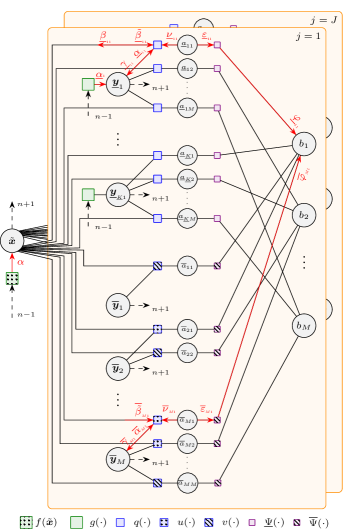
Figure 2: Factor graph for proposed algorithm. At MP iteration $p$, we use the following short hand notation: $f(\tilde{\bm{x}})\triangleq f(\tilde{\bm{x}}_{n}|\tilde{\bm{x}}_{n-1})$, $g(\cdot)$, $q(\cdot)$, $u(\cdot)$, $v(\cdot)$, $\underline{\Psi}(\cdot)$ and $\overline{\Psi}(\cdot)$ corresponds to (22), (24), (25), (26), (27) and (28), respectively. Furthermore, we define $\alpha\triangleq\alpha(\tilde{\bm{x}}_{n})$, $\underline{\alpha}_{k}\triangleq\alpha(\underline{\bm{x}}^{(j)}_{k,n},\underline{r}^{(j)}_{k,n})$, $\underline{\alpha}_{kl}\triangleq\alpha_{l}(\underline{\bm{x}}^{(j)}_{k,n},\underline{r}^{(j)}_{k,n})$, $\overline{\alpha}_{kl}\triangleq\alpha_{l}(\overline{\bm{x}}^{(j)}_{k,n},\overline{r}^{(j)}_{k,n})$, $\underline{\varepsilon}_{kl}\triangleq\varepsilon(\underline{a}^{(j)}_{kl,n})$, $\overline{\varepsilon}_{kl}\triangleq\varepsilon(\overline{a}^{(j)}_{kl,n})$, $\underline{\gamma}_{kl}\triangleq\gamma_{l}(\underline{\bm{x}}^{(j)}_{k,n},\underline{r}^{(j)}_{k,n})$, $\overline{\gamma}_{kl}\triangleq\gamma_{l}(\overline{\bm{x}}^{(j)}_{k,n},\overline{r}^{(j)}_{k,n})$, $\underline{\nu}_{kl}\triangleq\underline{\nu}_{kl}(\underline{a}^{(j)}_{kl,n})$, $\overline{\nu}_{kl}\triangleq\overline{\nu}_{kl}(\overline{a}^{(j)}_{kl,n})$, $\underline{\varphi}_{kl}\triangleq\underline{\varphi}_{kl}(b_{l,n})$ and $\overline{\varphi}_{kl}\triangleq\overline{\varphi}_{kl}(b_{l,n})$. Due to our proposed scheduling, both $\tilde{\beta}_{kl}$ and $\overline{\tilde{\beta}}_{ml}$ are defined to be $\alpha(\tilde{\bm{x}}_{n})$ according to (55). Furthermore, $\overline{\beta}_{ml}\triangleq 1$ and $\underline{\beta}_{kl}\triangleq\beta^{(j)}_{kl}(\tilde{\bm{x}}_{n})$ since the augmented agent state is only updated with messages from legacy PVAs. The time evolution of the agent state and VAs is indicated with dashed arrows.

V Proposed Sum-Product Algorithm

The factor graph in Fig. 2 has cycles, therefore we have to decide on a specific order of message computation [49, 52]. We use iterative MP with MP iteration $p\in\{1,\dots,P\}$ where $P$ is the maximum number of MP iterations. We choose the order according to the following rules: (i) messages are only sent forward in time; (ii) for each PA, messages are updated in parallel; (iii) along an edge connecting the augmented agent state variable node and a new PVA, messages are only sent from the former to the latter; (iv) the augmented agent state variable node is only updated at MP iteration $P$. The corresponding messages are shown in Fig. 2. Note, that this scheduling is suboptimal since the extrinsic messages of the augmented agent state are neglected. This calculation order is solely chosen to reduce the computational demand. With these rules, the message passing equations of the SPA [49] yield the following operations at each time step.

V-A Prediction Step

A prediction step is performed for the augmented agent state and all legacy VAs $k\in{\cal{K}}_{n-1}^{(j)}$. It has the form of

$$\alpha(\tilde{\bm{x}}_{n}) =\int f(\tilde{\bm{x}}_{n}|\tilde{\bm{x}}_{n-1})b(\tilde{\bm{x}}_{n-1})\mathrm{d}\tilde{\bm{x}}_{n-1}$$ (31)

$$\alpha(\underline{\bm{x}}^{(j)}_{k,n},\underline{r}^{(j)}_{k,n}) =\sum_{r^{(j)}_{k,n-1}\in\{0,1\}}\iint g(\underline{\bm{x}}^{(j)}_{k,n},\underline{r}^{(j)}_{k,n}|\bm{x}^{(j)}_{k,n-1},r^{(j)}_{k,n-1},\tilde{\bm{x}}_{n-1})$$

$$\times b(\bm{x}^{(j)}_{k,n-1},r^{(j)}_{k,n-1})b(\tilde{\bm{x}}_{n-1})\mathrm{d}\bm{x}^{(j)}_{k,n-1}\mathrm{d}\tilde{\bm{x}}_{n-1}$$ (32)

with $b(\tilde{\bm{x}}_{n-1})$ and $b(\bm{x}^{(j)}_{k,n-1},r^{(j)}_{k,n-1})$ denoting the beliefs of the augmented agent state and the legacy VA $k$ calculated at the previous time step, respectively. The summation in (32), can be further written as

$$\alpha(\underline{\bm{x}}^{(j)}_{k,n},\underline{r}^{(j)}_{k,n}=1) =p_{\text{s}}\iint e^{-\mu_{\text{m}}\big{(}\tilde{\bm{x}}_{n-1},\underline{\bm{x}}^{(j)}_{k,n}\big{)}}f(\underline{\bm{x}}^{(j)}_{k,n},1|\bm{x}^{(j)}_{k,n-1},1)$$

$$\times b(\bm{x}^{(j)}_{k,n-1},1)b(\tilde{\bm{x}}_{n-1})\mathrm{d}\bm{x}^{(j)}_{k,n-1}\mathrm{d}\tilde{\bm{x}}_{n-1}$$ (33)

and $\alpha(\underline{\bm{x}}^{(j)}_{k,n},\underline{r}^{(j)}_{k,n}=0)=\underline{\alpha}^{\text{n},(j)}_{k}f_{\text{d}}(\underline{\bm{x}}^{(j)}_{k,n})$ with

$$\underline{\alpha}^{\text{n},(j)}_{k} \triangleq\tilde{b}_{k,n-1}+(1-p_{\text{s}})\int b(\underline{\bm{x}}^{(j)}_{k,n-1},1)\mathrm{d}\underline{\bm{x}}^{(j)}_{k,n-1}$$

$$=\tilde{b}_{k,n-1}+(1-p_{\text{s}})(1-\tilde{b}_{k,n-1})$$ (34)

where $\tilde{b}_{k,n-1}=\int b(\underline{\bm{x}}^{(j)}_{k,n-1},0)\mathrm{d}\underline{\bm{x}}^{(j)}_{k,n-1}$ approximates the probability of non-existence of legacy VA $k$.

V-B Measurement Evaluation

The messages $\varepsilon^{[p]}(\underline{a}^{(j)}_{kl,n})$ sent from factor nodes $q(\tilde{\bm{x}}_{n},\underline{\bm{y}}^{(j)}_{k,n},\underline{a}^{(j)}_{kl,n},\bm{z}^{(j)}_{l,n})$ to variable nodes $\underline{a}^{(j)}_{kl,n}$ at MP iteration $p$ with $k\in\{1,\dots,K_{n-1}^{(j)}\}$ and $l\in\{1,\dots,M_{n}^{(j)}\}$ are defined as

$$\varepsilon^{[p]}(\underline{a}^{(j)}_{kl,n})= \iint\tilde{\beta}^{[p]}_{kl}(\tilde{\bm{x}}_{n})\alpha^{[p]}_{l}(\underline{\bm{y}}^{(j)}_{k,n})$$

$$\times q(\tilde{\bm{x}}_{n},\underline{\bm{y}}^{(j)}_{k,n},\underline{a}^{(j)}_{kl,n},\bm{z}^{(j)}_{l,n})\mathrm{d}\tilde{\bm{x}}_{n}\mathrm{d}\underline{\bm{y}}^{(j)}_{k,n}.$$ (35)

The messages from factor nodes $u(\tilde{\bm{x}}_{n},\overline{\bm{y}}^{(j)}_{k,n},\overline{a}^{(j)}_{kl,n},\bm{z}^{(j)}_{l,n})$ to variable nodes $\overline{a}^{(j)}_{kl,n}$ where $k\in\{1,\dots,M_{n}^{(j)}\}$ and $l\in\{1,\dots,M_{n}^{(j)}\}\backslash k$, are given as

$$\varepsilon^{[p]}(\overline{a}^{(j)}_{kl,n})= \iint\tilde{\beta}^{[p]}_{kl}(\tilde{\bm{x}}_{n})\alpha^{[p]}_{l}(\overline{\bm{y}}^{(j)}_{k,n})$$

$$\times u(\tilde{\bm{x}}_{n},\overline{\bm{y}}^{(j)}_{k,n},\overline{a}^{(j)}_{kl,n},\bm{z}^{(j)}_{l,n})\mathrm{d}\tilde{\bm{x}}_{n}\mathrm{d}\overline{\bm{y}}^{(j)}_{k,n}$$ (36)

and the messages from factor nodes $v(\tilde{\bm{x}}_{n},\overline{\bm{y}}^{(j)}_{m,n},\overline{a}^{(j)}_{mm,n},\bm{z}^{(j)}_{m,n})$ to variable nodes $\overline{a}^{(j)}_{mm,n}$, $m\in\{1,\dots,M_{n}^{(j)}\}$, are given as

$$\varepsilon^{[p]}(\overline{a}^{(j)}_{mm,n})= \iint\tilde{\beta}^{[p]}_{mm}(\tilde{\bm{x}}_{n})\alpha^{[p]}_{m}(\overline{\bm{y}}^{(j)}_{m,n})$$

$$\times v(\tilde{\bm{x}}_{n},\overline{\bm{y}}^{(j)}_{m,n},\overline{a}^{(j)}_{mm,n},\bm{z}^{(j)}_{m,n})\mathrm{d}\tilde{\bm{x}}_{n}\mathrm{d}\overline{\bm{y}}^{(j)}_{m,n}.$$ (37)

Note that $\alpha^{[p=1]}_{l}(\underline{\bm{y}}^{(j)}_{k,n})\triangleq\alpha(\underline{\bm{x}}^{(j)}_{k,n},\underline{r}^{(j)}_{k,n})$ and $\alpha^{[p=1]}_{l}(\overline{\bm{y}}^{(j)}_{k,n})\triangleq 1$. For $p>1$, $\alpha^{[p]}_{l}({\bm{y}}^{(j)}_{k,n})$ is calculated according to Section V-E. The message $\tilde{\beta}^{[p]}_{kl}(\tilde{\bm{x}}_{n})$ will be defined in Section V-F. Using (35), $\varepsilon^{[p]}(\underline{a}^{(j)}_{kl,n})$ is further investigated. For the messages containing information about legacy VAs, it results in

$$\varepsilon^{[p]}(\underline{a}^{(j)}_{kl,n}=1)= \iint\tilde{\beta}^{[p]}_{kl}(\tilde{\bm{x}}_{n})\alpha^{[p]}_{l}(\underline{\bm{x}}^{(j)}_{k,n},\underline{r}^{(j)}_{k,n}=1)$$

$$\times\frac{\mu_{\text{m}}\big{(}\tilde{\bm{x}}_{n},\underline{\bm{x}}^{(j)}_{k,n}\big{)}f(\bm{z}^{(j)}_{l,n}|\tilde{\bm{x}}_{n},\underline{\bm{x}}^{(j)}_{k,n})}{\mu_{\text{fa}}f_{\text{fa}}(\bm{z}^{(j)}_{l,n})}\mathrm{d}\underline{\bm{x}}^{(j)}_{k,n}\mathrm{d}\tilde{\bm{x}}_{n}$$

$$\varepsilon^{[p]}(\underline{a}^{(j)}_{kl,n}=0)= \iint\tilde{\beta}^{[p]}_{kl}(\tilde{\bm{x}}_{n})\Big{(}\alpha^{[p]}_{l}(\underline{\bm{x}}^{(j)}_{k,n},\underline{r}^{(j)}_{k,n}=1)$$

$$\hskip 11.38109pt+\alpha^{[p]}_{l}(\underline{\bm{x}}^{(j)}_{k,n},\underline{r}^{(j)}_{k,n}=0)\Big{)}\mathrm{d}\underline{\bm{x}}^{(j)}_{k,n}\mathrm{d}\tilde{\bm{x}}_{n}.$$ (38)

This can be further simplify by dividing both messages by $\varepsilon^{[p]}(\underline{a}^{(j)}_{kl,n}=0)$. With an abuse of notation, it results in $\varepsilon^{[p]}(\underline{a}^{(j)}_{kl,n}=0)=1$.

The messages $\varepsilon^{[p]}(\overline{a}^{(j)}_{kl,n})$ can be obtained similarly by using (36) and (37), yielding

$$\varepsilon^{[p]}(\overline{a}^{(j)}_{kl,n}=1)=\iint\tilde{\beta}^{[p]}_{kl}(\tilde{\bm{x}}_{n})\alpha^{[p]}_{l}(\overline{\bm{x}}^{(j)}_{k,n},\overline{r}^{(j)}_{k,n}=1)$$

$$\hskip 5.69054pt\times\frac{f(\overline{\bm{x}}^{(j)}_{k,n}|\tilde{\bm{x}}_{n})\mu_{\text{m}}\big{(}\tilde{\bm{x}}_{n},\overline{\bm{x}}^{(j)}_{k,n}\big{)}f(\bm{z}^{(j)}_{l,n}|\tilde{\bm{x}}_{n},\overline{\bm{x}}^{(j)}_{k,n})}{\mu_{\text{fa}}f_{\text{fa}}(\bm{z}^{(j)}_{l,n})}\mathrm{d}\overline{\bm{x}}^{(j)}_{k,n}\mathrm{d}\tilde{\bm{x}}_{n}$$ (39)

$$\varepsilon^{[p]}(\overline{a}^{(j)}_{kl,n}=0)=\iint\tilde{\beta}^{[p]}_{kl}(\tilde{\bm{x}}_{n})\Big{(}\alpha^{[p]}_{l}(\overline{\bm{x}}^{(j)}_{k,n},\overline{r}^{(j)}_{k,n}=1)$$

$$\hskip 65.44133pt+\alpha^{[p]}_{l}(\overline{\bm{x}}^{(j)}_{k,n},\overline{r}^{(j)}_{k,n}=0)\Big{)}\mathrm{d}\overline{\bm{x}}^{(j)}_{k,n}\mathrm{d}\tilde{\bm{x}}_{n}$$ (40)

$$\varepsilon^{[p]}(\overline{a}^{(j)}_{mm,n}=1)=\iint\tilde{\beta}^{[p]}_{mm}(\tilde{\bm{x}}_{n})\alpha^{[p]}_{m}(\overline{\bm{x}}^{(j)}_{m,n},\overline{r}^{(j)}_{m,n}=1)$$

$$\times\frac{f(\overline{\bm{x}}^{(j)}_{m,n}|\tilde{\bm{x}}_{n})\mu_{\text{m}}\big{(}\tilde{\bm{x}}_{n},\overline{\bm{x}}^{(j)}_{m,n}\big{)}f(\bm{z}^{(j)}_{m,n}|\tilde{\bm{x}}_{n},\overline{\bm{x}}^{(j)}_{m,n})}{\mu_{\text{fa}}f_{\text{fa}}(\bm{z}^{(j)}_{m,n})}\mathrm{d}\overline{\bm{x}}^{(j)}_{m,n}\mathrm{d}\tilde{\bm{x}}_{n}$$ (41)

$$\varepsilon^{[p]}(\overline{a}^{(j)}_{mm,n}=0)=$$

$$\hskip 28.45274pt\iint\tilde{\beta}^{[p]}_{mm}(\tilde{\bm{x}}_{n})\alpha^{[p]}_{m}(\overline{\bm{x}}^{(j)}_{m,n},\overline{r}^{(j)}_{m,n}=0)\mathrm{d}\overline{\bm{x}}^{(j)}_{m,n}\mathrm{d}\tilde{\bm{x}}_{n}$$ (42)

The expressions can be simplified by dividing all messages by $\varepsilon(\overline{a}^{(j)}_{kl,n}=0)$. With an abuse of notation, it results in $\varepsilon(\overline{a}^{(j)}_{kl,n}=0)=1$ and

$$\varepsilon^{[p]}(\overline{a}^{(j)}_{mm,n}=0)$$

$$=\frac{\iint\tilde{\beta}^{[p]}_{mm}(\tilde{\bm{x}}_{n})\alpha^{[p]}_{m}(\overline{\bm{x}}^{(j)}_{m,n},0)\mathrm{d}\overline{\bm{x}}^{(j)}_{m,n}\mathrm{d}\tilde{\bm{x}}_{n}}{\iint\tilde{\beta}^{[p]}_{mm}(\tilde{\bm{x}}_{n})\Big{(}\alpha^{[p]}_{m}(\overline{\bm{x}}^{(j)}_{m,n},1)+\alpha^{[p]}_{m}(\overline{\bm{x}}^{(j)}_{m,n},0)\Big{)}\mathrm{d}\overline{\bm{x}}^{(j)}_{m,n}\mathrm{d}\tilde{\bm{x}}_{n}}$$ (43)

V-C Data Association

The messages $\varphi^{[p]}_{kl}(b^{(j)}_{l,n})$ sent from factor node $\Psi({a}^{(j)}_{kl},b^{(j)}_{l})$ to variable node $b^{(j)}_{l,n}$ and the message $\nu^{[p]}_{kl}(a^{(j)}_{kl,n})$ sent from factor node $\Psi({a}^{(j)}_{kl},b^{(j)}_{l})$ to variable node $a^{(j)}_{kl,n}$ are calculated using the measurement evaluation messages in (35), (36) and (37). Details can be found in Appendix B.

V-D Measurement update for PVAs

Next, we determine the messages sent from factor node $q(\tilde{\bm{x}}_{n},\underline{\bm{y}}^{(j)}_{k,n},\underline{a}^{(j)}_{kl},\bm{z}^{(j)}_{l,n})$ to variable node $\underline{\bm{y}}^{(j)}_{k,n}$ as

$$\gamma^{[p]}_{l}(\underline{\bm{y}}^{(j)}_{k,n}) =\sum_{\underline{a}^{(j)}_{kl,n}\in\{0,1\}}\int q(\tilde{\bm{x}}_{n},\underline{\bm{x}}^{(j)}_{k,n},\underline{r}^{(j)}_{k,n},\underline{a}^{(j)}_{kl,n},\bm{z}^{(j)}_{l,n})$$

$$\hskip 11.38109pt\times\underline{\nu}^{[p]}_{kl}(\underline{a}^{(j)}_{kl,n})\mathrm{d}\tilde{\bm{x}}_{n}$$ (44)

which results after marginalizing $\underline{a}^{(j)}_{kl,n}$ in

$$\gamma^{[p]}_{l}(\underline{\bm{x}}^{(j)}_{k,n},\underline{r}^{(j)}_{k}=1) =\int q(\tilde{\bm{x}}_{n},\underline{\bm{x}}^{(j)}_{k,n},1,1,\bm{z}^{(j)}_{l,n})\underline{\nu}^{[p]}_{kl}(1)\mathrm{d}\tilde{\bm{x}}_{n}$$

$$\hskip 11.38109pt+\underline{\nu}^{[p]}_{kl}(0)$$ (45)

$$\gamma^{[p]}_{l}(\underline{\bm{x}}^{(j)}_{k,n},\underline{r}^{(j)}_{k}=0) =\underline{\nu}^{[p]}_{kl}(0)\hskip 0.85358pt.$$ (46)

The messages from factor node $u(\tilde{\bm{x}}_{n},\overline{\bm{y}}^{(j)}_{k,n},\overline{a}^{(j)}_{kl},\bm{z}^{(j)}_{l,n})$ to variable node $\overline{\bm{y}}^{(j)}_{k,n}$ are given as

$$\gamma^{[p]}_{l}(\overline{\bm{y}}^{(j)}_{k,n}) =\sum_{\overline{a}^{(j)}_{kl,n}\in\{0,1\}}\int u(\tilde{\bm{x}}_{n},\overline{\bm{x}}^{(j)}_{k,n},\overline{r}^{(j)}_{k,n},\overline{a}^{(j)}_{kl,n},\bm{z}^{(j)}_{l,n})$$

$$\hskip 11.38109pt\times\overline{\nu}^{[p]}_{kl}(\overline{a}^{(j)}_{kl,n})\mathrm{d}\tilde{\bm{x}}_{n}$$ (47)

which results after marginalizing $\overline{a}^{(j)}_{kl,n}$ in

$$\gamma^{[p]}_{l}(\overline{\bm{x}}^{(j)}_{k,n},\overline{r}^{(j)}_{k}=1) =\int u(\tilde{\bm{x}}_{n},\overline{\bm{x}}^{(j)}_{k,n},1,1,\bm{z}^{(j)}_{l,n})\overline{\nu}^{[p]}_{kl}(1)\mathrm{d}\tilde{\bm{x}}_{n}$$

$$\hskip 11.38109pt+\overline{\nu}^{[p]}_{kl}(0)$$ (48)

$$\gamma^{[p]}_{l}(\overline{\bm{x}}^{(j)}_{k,n},\overline{r}^{(j)}_{k}=0) =\overline{\nu}^{[p]}_{kl}(0)\hskip 0.85358pt.$$ (49)

The message from factor node $v(\tilde{\bm{x}}_{n},\overline{\bm{y}}^{(j)}_{m,n},\overline{a}^{(j)}_{mm},\bm{z}^{(j)}_{m,n})$ to variable node $\overline{\bm{y}}^{(j)}_{m,n}$ is given by

$$\gamma^{[p]}_{m}(\overline{\bm{y}}^{(j)}_{m,n}) =\sum_{\overline{a}^{(j)}_{mm,n}\in\{0,1\}}\int v(\tilde{\bm{x}}_{n},\overline{\bm{y}}^{(j)}_{m,n},\overline{a}^{(j)}_{mm,n},\bm{z}^{(j)}_{m,n})$$

$$\hskip 28.45274pt\times\overline{\nu}^{[p]}_{mm}(\overline{a}^{(j)}_{mm,n})\mathrm{d}\tilde{\bm{x}}_{n}$$ (50)

resulting in

$$\gamma^{[p]}_{m}(\overline{\bm{x}}^{(j)}_{m,n},1) =\int v(\tilde{\bm{x}}_{n},\overline{\bm{x}}^{(j)}_{m,n},1,1,\bm{z}^{(j)}_{m,n})\overline{\nu}^{[p]}_{mm}(1)\mathrm{d}\tilde{\bm{x}}_{n}$$ (51)

$$\gamma^{[p]}_{m}(\overline{\bm{x}}^{(j)}_{m,n},0) =\overline{\nu}^{[p]}_{mm}(0)\hskip 0.85358pt.$$ (52)

The messages are initialized with $\gamma^{[p=1]}_{\ell}(\bm{y}^{(j)}_{k,n})=1$.

V-E Extrinsic Information

For each legacy VA, the messages sent from variable node $\underline{\bm{y}}^{(j)}_{k,n}$ to factor nodes $q(\tilde{\bm{x}}_{n},\underline{\bm{y}}^{(j)}_{k,n},\underline{a}^{(j)}_{kl,n};\bm{z}^{(j)}_{l,n})$ with $k\in{\cal{K}}^{(j)}_{n-1}$, $l\in{\cal{M}}^{(j)}_{n}$ at MP iteration $p+1$ are defined as

$$\alpha^{[p+1]}_{l}(\underline{\bm{y}}^{(j)}_{k,n}) =\alpha(\underline{\bm{y}}^{(j)}_{k,n})\prod_{\begin{subarray}{c}\ell=1\\ \ell\neq l\end{subarray}}^{M_{n}^{(j)}}\gamma^{[p]}_{\ell}(\underline{\bm{y}}^{(j)}_{k,n})\hskip 0.85358pt.$$ (53)

For new VAs, a similar expression can be obtained for the messages from variable node $\overline{\bm{y}}^{(j)}_{m,n}$ to factor nodes $u(\tilde{\bm{x}}_{n},\overline{\bm{y}}^{(j)}_{m,n},\overline{a}^{(j)}_{ml,n};\bm{z}^{(j)}_{l,n})$ and factor node $v(\tilde{\bm{x}}_{n},\overline{\bm{y}}^{(j)}_{m,n},\overline{a}^{(j)}_{mm,n};\bm{z}^{(j)}_{m,n})$, i.e.,

$$\alpha^{[p+1]}_{l}(\overline{\bm{y}}^{(j)}_{m,n}) =\alpha(\overline{\bm{y}}^{(j)}_{m,n})\prod_{\begin{subarray}{c}\ell=1\\ \ell\neq l\end{subarray}}^{m}\gamma^{[p]}_{\ell}(\overline{\bm{y}}^{(j)}_{m,n})\hskip 0.85358pt.$$ (54)

V-F Measurement update for augmented agent state

Due to the proposed scheduling, the augmented agent state is only updated by messages of legacy PVAs and only at the end of the iterative message passing. This results in

$$\tilde{\beta}^{[p]}_{kl}(\tilde{\bm{x}}_{n}) =\alpha(\tilde{\bm{x}}_{n})$$ (55)

$$\beta^{[p](j)}_{kl}(\tilde{\bm{x}}_{n}) =\sum_{\underline{a}^{(j)}_{kl,n}\in\{0,1\}}\sum_{\underline{r}^{(j)}_{k,n}\in\{0,1\}}\int\alpha_{l}^{[p]}(\underline{\bm{x}}^{(j)}_{k,n},\underline{r}^{(j)}_{k,n})$$

$$\times q(\tilde{\bm{x}}_{n},\underline{\bm{x}}^{(j)}_{k,n},\underline{r}^{(j)}_{k,n},\underline{a}^{(j)}_{kl,n},\bm{z}^{(j)}_{l,n})\underline{\nu}^{[p]}_{kl}(\underline{a}^{(j)}_{kl,n})\mathrm{d}\underline{\bm{x}}^{(j)}_{k,n}$$ (56)

which can be further simplified to

$$\beta^{[p](j)}_{kl}(\tilde{\bm{x}}_{n}) =\int\alpha_{l}^{[p]}(\bm{x}^{(j)}_{k,n},1)\Big{(}q(\tilde{\bm{x}}_{n},\underline{\bm{x}}^{(j)}_{k,n},1,1,\bm{z}^{(j)}_{l,n})\underline{\nu}^{[p]}_{kl}(1)$$

$$\hskip 8.53581pt+\underline{\nu}^{[p]}_{kl}(0)\Big{)}\mathrm{d}\underline{\bm{x}}^{(j)}_{k,n}+\underline{\alpha}_{k}^{\text{n},(j)}\underline{\nu}^{[p]}_{kl}(0).$$ (57)

V-G Belief calculation

Once all messages are available and $p=P$, the beliefs approximating the desired marginal posterior PDFs are obtained. The belief for the augmented agent state is given, up to a normalization factor, by

$$b(\tilde{\bm{x}}_{n})\propto\alpha(\tilde{\bm{x}}_{n})\prod_{j=1}^{J}\ \prod_{k=1}^{K_{n-1}^{(j)}}\ \prod_{m=1}^{M_{n}^{(j)}}\beta^{[P](j)}_{km}(\tilde{\bm{x}}_{n})$$ (58)

where we only use messages from legacy VAs. This belief (after normalization) provides an approximation of the marginal posterior PDF $f(\tilde{\bm{x}}_{n}|\bm{z}_{1:n})$, and it is used instead of $f(\tilde{\bm{x}}_{n}|\bm{z}_{1:n})$ in (29). Furthermore, the beliefs of the legacy VAs $b(\underline{\bm{y}}^{(j)}_{k})$ and new VAs $b(\overline{\bm{y}}^{(j)}_{k})$ are given as

$$b(\underline{\bm{y}}^{(j)}_{k,n}) \propto\alpha(\underline{\bm{y}}^{(j)}_{k,n})\prod_{l=1}^{M_{n}^{(j)}}\gamma^{[P]}_{l}(\underline{\bm{y}}^{(j)}_{k,n})$$ (59)

$$b(\overline{\bm{y}}^{(j)}_{m,n}) \propto\alpha(\overline{\bm{y}}^{(j)}_{m,n})\prod_{l=1}^{m}\gamma^{[P]}_{l}(\overline{\bm{y}}^{(j)}_{m,n})$$ (60)

A computationally feasible approximate calculation of the various messages and beliefs can be based on the sequential Monte Carlo (particle-based) implementation approach introduced in [50, 26, 22].

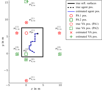
Figure 3: Considered scenario for performance evaluation in a rectangular room with two PAs, four reflective surfaces and the corresponding VAs. The estimated agent track for a single realization is shown in blue.

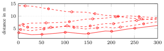
(a)

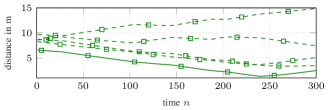
(b)

(c)

Figure 4: Distances of main components (between the PA positions as well as their corresponding VA positions and the agent positions) versus time $n$.

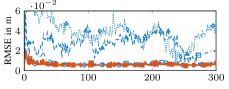
(a)

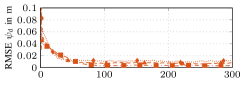
(b)

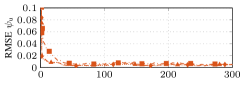
(c)

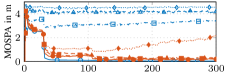
(d)

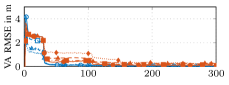
(e)

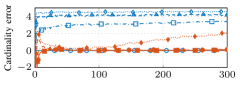
(f)

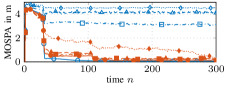
(g)

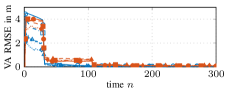
(h)

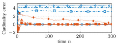
(i)

(j)

Figure 5: Experiment 1: Results for converged simulation runs. (a) shows the RMSE of the agent position over the whole track. (b) and (c) present the RMSE of the dispersion parameters. (d) and (g) present the map error in terms of the MOSPA for PA $1$ and PA $2$, respectively. (e) and (h) show the RMSE of the estimated VA positions for PA $1$ and PA $2$, respectively. (f) and (i) show the cardinality error of the estimated VAs for PA $1$ and PA $2$, respectively.

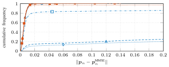
Figure 6: Experiment 1: Cumulative frequency of the deviation of the MMSE estimate of the agent position from the true agent position for all simulation runs and time instances. The legend is given in Fig. 5.

VI Numerical Results

The performance of the proposed algorithm (PROP) is validated and compared with the MP-SLAM from [3, 11], which assumes that each VA generates at most one measurement and that a measurement originates from at most one VA. The validation of the algorithms is based on synthetic measurements in two settings.

1. Experiment 1 in Section VI-B is based on measurements directly generated from the measurement model introduced in Section IV.

2. Experiment 2 in Section VI-C is based on measurements provided by a CEDA applied to radio signals that are generated with parameters according to the measurement model introduced in Section IV.

VI-A Simulation Scenario and Common Simulation Parameters

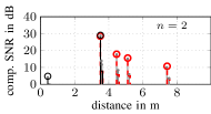
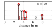
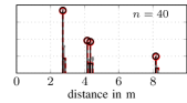
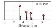
(a)

Figure 7: Estimated distances and dispersion parameters for PA $1$ for a single simulation run, represented by dot markers and boxes, respectively. The true components and respective dispersion parameters are indicated in red. All measurements are indicated in gray. Estimated components and respective dispersion parameters are indicated in black.

We consider an indoor scenario shown in Fig. 3. The scenario consists of two PAs at positions $\bm{p}_{\mathrm{pa}}^{(1)}=[0.1\hskip 2.84526pt6]^{\text{T}}$, and $\bm{p}_{\mathrm{pa}}^{(2)}=[0\hskip 2.84526pt-0.2]^{\text{T}}$ and four reflective surfaces, i.e., $4$ VAs per PA. The agent moves along a track which is observed for $300$ time instances $n$ with observation period $\Delta T=1\,$s. For simplicity, we restrict the simulations to single-bounce reflections. The distances of the main components are calculated based on the PA and the corresponding VAs positions as well as agent positions (see Section III). Fig. 4 shows the distances of the main components versus time $n$. The signal SNR is set to $30\,\mathrm{dB}$ at an LOS distance of $1\,$m. The amplitudes of the main components (LOS component and the MPCs) are calculated using a free-space path loss model and an additional attenuation of $1\,\mathrm{dB}$ for each reflection at a flat surface. We use $20000$ particles. The particles for the initial agent state are drawn from a 4-D uniform distribution with center $\bm{x}_{0}=[\bm{p}_{0}^{\text{T}}\;0\;\,0]^{\text{T}}$, where $\bm{p}_{0}$ is the starting position of the actual agent track, and the support of each position component about the respective center is given by $[-0.1\,\mathrm{m},0.1\,\mathrm{m}]$ and of each velocity component is given by $[-0.01\,\mathrm{m/s},0.01\,\mathrm{m/s}]$. At time $n=0$, the number of VAs is $0$, i.e., no prior map information is available. The prior distribution for new PVA states $f_{\text{n}}\big{(}\overline{\bm{x}}^{(j)}_{m,n}|\tilde{\bm{x}}_{n}\big{)}$ is uniform on the square region given by $[-\text{15 m},\text{15 m}]\times[-\text{15 m},\text{15 m}]$ around the center of the floor plan shown in Fig. 3 and the mean number of new PVAs at time $n$ is $\mu_{\text{n}}=0.01$. The probability of survival is $p_{\mathrm{s}}=0.999$. The confirmation threshold as well as the pruning threshold are given as $p_{\mathrm{cf}}=0.5$ and $p_{\mathrm{pr}}=10^{-3}$, respectively. For the sake of numerical stability, we introduce a small amount of regularization noise to the VA state $\bm{p}_{k,\mathrm{va}}$ at each time step $n$, i.e., $\underline{\bm{p}}^{(j)}_{k,\mathrm{va}}=\bm{p}^{(j)}_{k,\mathrm{va}}+\bm{\omega}_{k}$, where $\bm{\omega}_{k}$ is iid across $k$, zero-mean, and Gaussian with covariance matrix $\sigma_{a}^{2}\,\mathbb{I}_{2}$ and $\sigma_{a}=10^{-3}\,\text{m}$. The state transition variances are set as $\sigma_{\text{w}}=10^{-3}\,\mathrm{m/s^{2}}$, $q_{\tau}=q_{\text{u}}=10^{4}$ [27, 24], and $\sigma_{\text{u},k}=0.05\,u_{k,n-1}^{(j)\hskip 0.5pt\text{MMSE}}$. Note that for the normalized amplitude state, we use a value proportional to the MMSE estimate of the previous time step $n-1$ as a heuristic. The dispersion parameters are set to fixed values over time $n$, i.e., ${\psi}_{\tau,n}=\psi_{\tau}=\psi_{\text{d}}/c$ and ${\psi}_{\text{u},n}={\psi}_{\text{u}}$. The performance of the different methods discussed is measured in terms of the RMSE of the agent position and the dispersion parameters as well as the optimal subpattern assignment (OSPA) error [53] of all VAs with cutoff parameter and order set to 5 m and 2, respectively. The MOSPA errors and RMSEs of each unknown variable are obtained by averaging over all converged simulation runs. We declare a simulation run to be converged if $\{\forall n:\|\bm{p}_{n}-\bm{p}^{\text{MMSE}}_{n}\|<d_{\text{cv}}\,\text{m}\}$, where $d_{\text{cv}}$ is the convergence threshold.

VI-B Experiment 1: Measurement Model

We investigate PROP with four different dispersion parameter settings, given as $\psi_{\text{d}}$, which takes values of $0\,$m, $0.03\,$m, $0.15\,$m and $0.3\,$m, and ${\psi}_{\text{u}}$, which is either set to $0$ for $\psi_{\text{d}}=0\,$m or $0.2$ otherwise. Furthermore, we set $N_{\text{ny}}=4$. We performed $100$ simulation runs. In each simulation run, we generated noisy measurements $\bm{z}_{m,n}^{(j)}$ according to the measurement model proposed in Section IV-B using the main components calculated as described in Section VI-A. In the case $\psi_{\text{d}}=0\,\mathrm{m}$ only main-component measurements are generated, which is equivalent to the system model in [11]. The detection threshold is given by $\gamma=2.5$. For numerical stability, we reduced the root mean squared bandwidth $\beta_{\text{bw}}$ for VAs by a factor of $4$. The convergence threshold is set to $d_{\text{cv}}=0.2$.

TABLE I: Experiment 1: Convergence rate and mean number of estimated VAs for different algorithms and dispersion settings.

	setting	convergence	$\hat{K}$
MP-SLAM	$\psi_{\text{d}}=0.00\,\mathrm{m}$	100 %	4
	$\psi_{\text{d}}=0.03\,\mathrm{m}$	82 %	9
	$\psi_{\text{d}}=0.15\,\mathrm{m}$	15 %	16
	$\psi_{\text{d}}=0.30\,\mathrm{m}$	11 %	30
PROP	$\psi_{\text{d}}=0.00\,\mathrm{m}$	100 %	4
	$\psi_{\text{d}}=0.03\,\mathrm{m}$	100 %	4
	$\psi_{\text{d}}=0.15\,\mathrm{m}$	100 %	4
	$\psi_{\text{d}}=0.30\,\mathrm{m}$	96 %	5

Table I summarizes the number of converged runs (in percentage) as well as the mean number of detected VAs $\hat{K}$ (averaged over all simulation runs and time steps) for all investigated dispersion parameter settings. The results are summarized in Fig. 5. In particular, Fig. 5a shows the RMSE of the agent positions, Fig. 5b and 5c show the RMSE of the dispersion parameters, Fig. 5d - Fig. 5f as well as Fig. 5g - Fig. 5i show the MOSPA error and its VA position error and mean cardinality error contributions for PA $1$ and PA $2$, respectively. The results in all figures are presented versus time $n$ (and for all investigated dispersion parameter settings). Fig. 5a shows that the RMSE of the agent position of PROP is similar for all dispersion parameter settings. While PROP significantly outperforms MP-SLAM in terms of converged runs for dispersion parameter settings $\psi_{\text{d}}>0\,\mathrm{m}$, it shows slightly reduced performance for $\psi_{\text{d}}=0\,\mathrm{m}$. Additionally, Fig. 6 shows the cumulative frequencies of the individual agent errors, i.e., $\|\bm{p}_{n}-\bm{p}^{\text{MMSE}}_{n}\|$ for all simulation runs and time instances. It can be observed that the MMSE positions of the agent of PROP show almost no large deviations, while the estimates of MP-SLAM exhibit large errors in many simulation runs. For dispersion parameter settings $\psi_{\text{d}}>0\,\mathrm{m}$, measurements of the sub-components are available. Thus, as Fig. 5b and 5c show, the dispersion parameters are well estimated indicated by the small RMSEs. For the setting $\psi_{\text{d}}=0\,\mathrm{m}$, estimation of the dispersion parameters is not possible because there are no sub-component measurements, i.e., there is only one measurement generated by each VA. However, as Fig. 5a shows, this does not affect the accuracy of the agent’s position estimation.

The MOSPA errors (and their VA positions and the mean cardinality error contributions) of PROP, shown in Fig. 5d and 5g, are very similar for all dispersion parameter settings. They slightly increase with increased dispersion parameter $\psi_{\text{d}}$. Only for the setting $\psi_{\text{d}}=0.3\,\mathrm{m}$, PROP shows a larger cardinality error. This can be explained by looking at the distances from PA $1$ and its corresponding VAs as shown in Fig. 4. At the end of the agent track, many VAs show similar distances to the agent’s position making it difficult to resolve the individual components. For larger dispersion parameter $\psi_{\text{d}}$, this becomes even more challenging leading to increased MOSPA errors. For PA $2$ and the corresponding VAs, Fig. 4 shows that all components are well separated by their distances at the end of the agent track, which makes it easier for PROP to correctly estimate the number and positions of VAs. Unlike PROP, MP-SLAM completely fails to estimate the correct number of VAs for larger $\psi_{\text{d}}$ (and ${\psi}_{\text{u}}$), resulting in a large cardinality error. This can be explained by the fact that MP-SLAM does not consider additional sub-components in the measurement and system model. We suspect that this estimation of additional spurious VAs is the reason for the large number of divergent simulation runs. As an example, Fig. 7 depicts the time evolution of the estimated distances (using the PA position, the estimated VA positions, and estimated agent positions) with according component SNRs as well as the respective dispersion parameters for PA $1$.

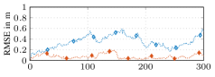
(a)

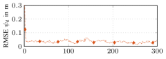
(b)

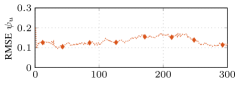
(c)

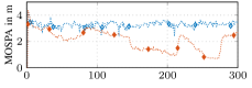
(d)

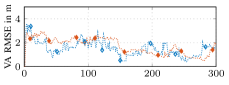
(e)

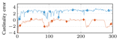
(f)

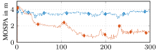
(g)

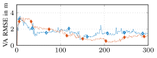
(h)

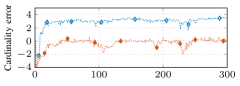
(i)

(j)

Figure 8: Experiment 2: Results for converged simulation runs based on estimates from CEDA. (a) shows the RMSE of the agent position over the whole track. (b) and (c) present the RMSE of the dispersion parameters. (d) and (g) present the map error in terms of the MOSPA for PA $1$ and PA $2$, respectively. (e) and (h) show the RMSE of the estimated VA positions for PA $1$ and PA $2$, respectively. (f) and (i) show the cardinality error of the estimated VAs for PA $1$ and PA $2$, respectively.

VI-C Experiment 2: Radio Signals

In this section, we use a dispersion parameter setting of $\psi_{\text{d}}=0.3\,\mathrm{m}$ and $\psi_{\text{u}}=0.2$. The signal spectrum of the transmit pulse $s(t)$ has a root-raised-cosine shape with a roll-off factor of $0.6$ and a $3\,\mathrm{dB}$ bandwidth of $B=1\,\mathrm{GHz}$. The signal is critically sampled, i.e., $T_{\text{s}}=1/(1.6B)$, with a total number of $N_{\text{s}}=161$ samples resulting in a maximum distance $d_{\text{max}}=60\,\mathrm{m}$. For the data generation, we use $N_{\text{ny}}=2$. We perform $10$ simulation runs. In each simulation run, we generate a received signal vector (see (6)) using the main components calculated as described in Section VI-A and uniformly distributed sub-components (see (IV-B)). To obtain the measurements, we use the CEDA in [19] with a detection threshold of $\gamma=2$, i.e., corresponding to $6\,\mathrm{dB}$ [23]. For numerical stability, we reduced the root mean squared bandwidth $\beta_{\text{bw}}$ for VAs by a factor of $4$ and increased the factor $1/2$ in amplitude scale parameter in (13) to $4$. The convergence threshold is $d_{\text{cv}}=2$.

TABLE II: Experiment 2: Convergence rate and mean number of estimated VAs for different algorithms.

setting	convergence	$\hat{K}$
MP-SLAM $\psi_{\text{d}}=0.30\,\mathrm{m}$	20 %	7.5
PROP $\psi_{\text{d}}=0.30\,\mathrm{m}$	100 %	3.7

Table II again summarizes the number of converged runs and the mean number of detected VAs. For PROP, none of the simulation runs diverged, but $80\,\%$ of the MP-SLAMs simulation runs diverged, showing that PROP significantly outperforms MP-SLAM. The results shown in Fig. 8 follow a similar trend as the results shown in Fig. 5. The only significant difference is observed in the RMSE of the dispersion parameter $\psi_{\text{u}}$, which remains relatively large (see Fig. 8c). This is because the variance of the estimated normalized amplitudes provided by the CEDA is very large. This may be explained by two factors: (i) the CEDA also needs to estimate the noise variance, which is only approximately covered by the amplitude scale parameter given in (13), and (ii) the sub-components are very close in the delay domain, resulting in strongly correlated amplitude estimates. The steps in Fig. 8d and 8f are due to crossings where the delays from two or more VAs to the agent are equal. Hence, one of the VAs is discarded, leading to an overall underestimated number of VAs.

VII Conclusions

We have proposed a new MP-SLAM method that can cope with multiple-measurements being generated by a single environment feature, i.e., a single VA. It is based on a novel statistical measurement model that is derived from the radio signal introducing dispersion parameters to MPCs. The resulting likelihood function model allows to capture the measurement spread originating from non-ideal effects such as rough reflective surfaces or non-calibrated antennas. The performance results show that the proposed method is able to cope with multiple measurements being produced per VA and outperforms classical MP-SLAM in terms of the agent positioning error and the map MOSPA error. We show that multiple measurements get correctly associated to their corresponding VA, resulting in a correctly estimated number of VAs. Furthermore, the results indicate that the proposed algorithm generalizes to the classical multipath-based SLAM for a single measurement per VA. Possible directions of future research include the extension to individual dispersion parameters for each feature as well as incorporating multiple-measurements-to-feature data association into the MVA-based SLAM method [46].

Appendix A Radio Signal Model

In this section we derive the radio signal model described in Section III. Usually, specular reflections of radio signals at flat surfaces are modeled by VAs that are mirror images of the PAs [1, 2, 3, 4]. We start by defining the typical channel impulse response, given for time $n$ and anchor $j$ as

$$h_{\text{c},n}^{(j)}(\tau)=\sum_{l=1}^{{L}_{n}^{(j)}}{\alpha}_{l,n}^{(j)}\delta\big{(}\tau-{\tau}_{l,n}^{(j)}\big{)}\hskip 0.85358pt.$$ (61)

The first summand describes the LOS component and the sum of ${L}_{n}^{(j)}-1$ the specular MPCs with their corresponding complex amplitudes ${\alpha}_{l,n}^{(j)}$ and delays ${\tau}_{l,n}^{(j)}$, respectively. In non-ideal radio channels we observe rays to arrive as clusters [54, 6, 55, 7]. The reason for this observation is manifold. Typical examples are non-calibrated antennas, the scattering from a user-body as well as non-ideal reflective surfaces. Fig. 1 visualizes these effects, introducing generic impulse responses $h_{\text{ant},n}^{(j)}(\tau)$ and $h_{\text{surf},n}^{(j)}(\tau)$. We propose to model the overall impulse response encompassing all considered dispersion effects as

$$\vspace{-2mm}h_{\text{d},n}^{(j)}(\tau)=\delta(\tau)+\sum_{i=1}^{S_{l}^{(j)}}\beta^{(j)}_{l,i,n}\delta(\tau-\nu^{(j)}_{l,i,n}\big{)}$$ (62)

where $\beta^{(j)}_{l,i,n}\in\mathbb{R}$ is a relative dampening variable and $\nu^{(j)}_{l,i,n}$ is the excess delay. The presented model denotes a marked Possion point process [55]. Its statistical properties, i.e, the distribution of $\nu^{(j)}_{l,i,n}$, $\beta^{(j)}_{l,i,n}$, and $S_{l}^{(j)}$, are discussed in Section III and IV in detail. We obtain the complex baseband signal received at the $j$th anchor given by the convolution of $h_{\text{d},n}^{(j)}(\tau)$ and $h_{\text{c},n}^{(j)}(\tau)$ with the transmitted signal $s(t)$ as

$$\bm{\mathsfbr{s}}_{\text{rx},n}^{(j)} =\sum_{l=1}^{{L}_{n}^{(j)}}{\alpha}_{l,n}^{(j)}\Big{(}s(t-{\tau}_{l,n}^{(j)})$$

$$\hskip 8.53581pt+\sum_{i=1}^{S_{l}^{(j)}}\beta^{(j)}_{l,i,n}s(t-{\tau}_{l,n}^{(j)}-\nu^{(j)}_{l,i,n})\Big{)}+\mathsfbr{n{}}_{n}^{(j)}(t)\hskip 0.85358pt.$$ (63)

The second term $\mathsfbr{n{}}_{n}^{(j)}(t)$ represents an additive white Gaussian noise process with double-sided power spectral density ${N}_{0}^{(j)}/\hskip 0.5pt2$.

Appendix B Data Association

This section contains the detailed derivation of the data association-related messages $\varphi^{[p]}_{kl}(b^{(j)}_{l,n})$ and $\nu^{[p]}_{kl}(a^{(j)}_{kl,n})$. Using the measurement evaluation messages in (35), (36) and (37), the messages $\underline{\varphi}^{[p]}_{kl}(b^{(j)}_{l,n})$ and $\overline{\varphi}^{[p]}_{ml}(b^{(j)}_{l,n})$ are calculated by

$$\underline{\varphi}^{[p]}_{kl}(b^{(j)}_{l,n}) =\sum_{\underline{a}^{(j)}_{kl,n}\in\{0,1\}}\varepsilon^{[p]}(\underline{a}^{(j)}_{kl,n})\underline{\Psi}(\underline{a}^{(j)}_{kl,n},b^{(j)}_{l,n})$$ (64)

$$\overline{\varphi}^{[p]}_{ml}(b^{(j)}_{l,n}) =\sum_{\overline{a}^{(j)}_{ml,n}\in\{0,1\}}\varepsilon^{[p]}(\overline{a}^{(j)}_{ml,n})\overline{\Psi}(\overline{a}^{(j)}_{ml,n},b^{(j)}_{l,n})$$ (65)

for $k\in\{1,\dots,\underline{K}\}$ with $\underline{K}\triangleq K^{(j)}_{n-1}$ and $m,l\in\{1,\dots,M^{(j)}_{n}\}$ and are sent from factor node $\underline{\Psi}(\underline{a}^{(j)}_{kl,n},b^{(j)}_{l,n})$ and $\overline{\Psi}(\overline{a}^{(j)}_{ml,n},b^{(j)}_{l,n})$ to variable node $b^{(j)}_{l,n}$, respectively. By making use of the indicator functions given in (27) and (28), respectively, (64) and (65) are also given as

$$\underline{\varphi}^{[p]}_{kl}(b^{(j)}_{l,n}=k) =\varepsilon^{[p]}(\underline{a}^{(j)}_{kl,n}=1)$$ (66)

$$\underline{\varphi}^{[p]}_{kl}(b^{(j)}_{l,n}\neq k) =\varepsilon^{[p]}(\underline{a}^{(j)}_{kl,n}=0)$$ (67)

$$\overline{\varphi}^{[p]}_{ml}(b^{(j)}_{l,n}=\underline{K}+m) =\varepsilon^{[p]}(\overline{a}^{(j)}_{ml,n}=1)$$ (68)

$$\overline{\varphi}^{[p]}_{ml}(b^{(j)}_{l,n}\neq\underline{K}+m) =\varepsilon^{[p]}(\overline{a}^{(j)}_{ml,n}=0)$$ (69)

The messages in (66) - (69) can be rewritten in the form of

$$\underline{\varphi}^{[p]}_{kl}(b^{(j)}_{l,n}) =\begin{cases}\frac{\varepsilon^{[p]}(\underline{a}^{(j)}_{kl,n}=1)}{\varepsilon^{[p]}(\underline{a}^{(j)}_{kl,n}=0)},&b^{(j)}_{l,n}=k\\ 1,&b^{(j)}_{l,n}\neq k\end{cases}$$ (70)

$$\overline{\varphi}^{[p]}_{ml}(b^{(j)}_{l,n}) =\begin{cases}\frac{\varepsilon^{[p]}(\overline{a}^{(j)}_{ml,n}=1)}{\varepsilon^{[p]}(\overline{a}^{(j)}_{ml,n}=0)},&b^{(j)}_{l,n}=\underline{K}+m\\ 1,&b^{(j)}_{l,n}\neq\underline{K}+m.\end{cases}$$ (71)

The messages $\underline{\nu}^{[p]}_{kl}(\underline{a}^{(j)}_{kl,n})$ and $\overline{\nu}^{[p]}_{ml}(\overline{a}^{(j)}_{ml,n})$ represent the messages from variable node $\underline{a}^{(j)}_{kl,n}$ to factor node $q(\tilde{\bm{x}}_{n},{\underline{\bm{y}}}^{(j)}_{k,n},\underline{a}^{(j)}_{kl,n};\bm{z}^{(j)}_{l,n})$ and from variable node $\overline{a}^{(j)}_{ml,n}$ to factor node $u(\tilde{\bm{x}}_{n},{\overline{\bm{y}}}^{(j)}_{m,n},\overline{a}^{(j)}_{ml,n};\bm{z}^{(j)}_{l,n})$, respectively. $\overline{\nu}^{[p]}_{mm}(\overline{a}^{(j)}_{mm,n})$ represents the messages from variable node $\overline{a}^{(j)}_{mm,n}$ to factor node $v(\tilde{\bm{x}}_{n},{\overline{\bm{y}}}^{(j)}_{m,n},\overline{a}^{(j)}_{mm,n};\bm{z}^{(j)}_{m,n})$. They are defined as

$$\underline{\nu}^{[p]}_{kl}(\underline{a}^{(j)}_{kl,n}) =\sum_{b^{(j)}_{l,n}=0}^{K^{(j)}_{n}}\prod_{\begin{subarray}{c}i=1\\ i\neq k\end{subarray}}^{\underline{K}}\underline{\varphi}^{[p]}_{il}(b^{(j)}_{l,n})\prod_{m=l}^{M^{(j)}_{n}}\overline{\varphi}^{[p]}_{ml}(b^{(j)}_{l,n})$$ (72)

$$\overline{\nu}^{[p]}_{ml}(\overline{a}^{(j)}_{ml,n}) =\sum_{b^{(j)}_{l,n}=0}^{K^{(j)}_{n}}\prod_{i=1}^{\underline{K}}\underline{\varphi}^{[p]}_{il}(b^{(j)}_{l,n})\prod_{\begin{subarray}{c}h=l\\ h\neq m\end{subarray}}^{M^{(j)}_{n}}\overline{\varphi}^{[p]}_{hl}(b^{(j)}_{l,n}).$$ (73)

Using the results from (70) and (71), (72) and (73) are, respectively, rewritten as

$$\underline{\nu}^{[p]}_{kl}(\underline{a}^{(j)}_{kl,n}=1)= \prod_{\begin{subarray}{c}i=1\\ i\neq k\end{subarray}}^{\underline{K}}\underline{\varphi}^{[p]}_{il}(b^{(j)}_{l,n}=k)\prod_{m=l}^{M^{(j)}_{n}}\overline{\varphi}^{[p]}_{ml}(b^{(j)}_{l,n}=\underline{K}+k)$$

(74)

$$\underline{\nu}^{[p]}_{kl}(\underline{a}^{(j)}_{kl,n}=0)= \sum_{\begin{subarray}{c}b^{(j)}_{l,n}=0\\ b^{(j)}_{l,n}\notin\{k,\underline{K}+k\}\end{subarray}}^{K^{(j)}_{n}}\prod_{\begin{subarray}{c}i=1\\ i\neq k\end{subarray}}^{\underline{K}}\underline{\varphi}^{[p]}_{il}(b^{(j)}_{l,n})\prod_{m=l}^{M^{(j)}_{n}}\overline{\varphi}^{[p]}_{ml}(b^{(j)}_{l,n})$$

and

$$\overline{\nu}^{[p]}_{ml}(\overline{a}^{(j)}_{ml,n}=1)= \prod_{i=1}^{\underline{K}}\underline{\varphi}^{[p]}_{il}(b^{(j)}_{l,n}=m)\prod_{\begin{subarray}{c}h=l\\ h\neq m\end{subarray}}^{M^{(j)}_{n}}\overline{\varphi}^{[p]}_{hl}(b^{(j)}_{l,n}=\underline{K}+m)$$

(76)

$$\overline{\nu}^{[p]}_{ml}(\overline{a}^{(j)}_{ml,n}=0)= \sum_{\begin{subarray}{c}b^{(j)}_{l,n}=0\\ b^{(j)}_{l,n}\notin\{m,\underline{K}+m\}\end{subarray}}^{K^{(j)}_{n}}\prod_{i=1}^{\underline{K}}\underline{\varphi}^{[p]}_{il}(b^{(j)}_{l,n})\prod_{\begin{subarray}{c}h=l\\ h\neq m\end{subarray}}^{M^{(j)}_{n}}\overline{\varphi}^{[p]}_{hl}(b^{(j)}_{l,n})$$

Note that $\varphi^{[p]}_{kl}(b^{(j)}_{l,n}=0)=1$. By normalizing (74) by $\underline{\nu}^{[p]}_{kl}(\underline{a}^{(j)}_{kl,n}=0)$ and (76) by $\overline{\nu}^{[p]}_{ml}(\overline{a}^{(j)}_{ml,n}=0)$, equivalent expressions for (72) and (73) are given as

$$\underline{\nu}^{[p]}_{kl}(\underline{a}^{(j)}_{kl,n})$$

$$=\begin{cases}\frac{\prod_{\begin{subarray}{c}{$i=1$}\\ {$i\neq k$}\end{subarray}}^{\underline{K}}\underline{\varphi}^{[p]}_{il}(b^{(j)}_{l,n}=k)\prod_{m=l}^{M}\overline{\varphi}^{[p]}_{ml}(b^{(j)}_{l,n}=\underline{K}+k)}{\sum_{\begin{subarray}{c}{$b^{(j)}_{l,n}=0$}\\ {$b^{(j)}_{l,n} \notin\{k,\text@underline{K} + k\}$}\end{subarray}}^{K^{(j)}_{n}}\prod_{\begin{subarray}{c}{$i=1$}\\ {$i\neq k$}\end{subarray}}^{\underline{K}}\underline{\varphi}^{[p]}_{il}(b^{(j)}_{l,n})\prod_{m=l}^{M^{(j)}_{n}}\overline{\varphi}^{[p]}_{ml}(b^{(j)}_{l,n})},&\underline{a}^{(j)}_{kl,n}=1\\ 1,&\underline{a}^{(j)}_{kl,n}=0.\end{cases}$$ (78)

$$\overline{\nu}^{[p]}_{ml}(\overline{a}^{(j)}_{ml,n})$$

$$=\begin{cases}\hskip 2.84526pt\frac{\prod_{i=1}^{\underline{K}}\underline{\varphi}^{[p]}_{il}(b^{(j)}_{l,n}=m)\prod_{\begin{subarray}{c}{$h=l$}\\ {$h\neq m$}\end{subarray}}^{M^{(j)}_{n}}\overline{\varphi}^{[p]}_{hl}({$b^{(j)}_{l,n} = \text@underline{K} + m$})}{\sum_{\begin{subarray}{c}{$b^{(j)}_{l,n}=0$}\\ {$b^{(j)}_{l,n} \notin\{m,\text@underline{K} + m\}$}\end{subarray}}^{K^{(j)}_{n}}\prod_{i=1}^{\underline{K}}\underline{\varphi}^{[p]}_{il}({$b^{(j)}_{l,n}$})\prod_{\begin{subarray}{c}{$h=l$}\\ {$h\neq m$}\end{subarray}}^{M^{(j)}_{n}}\overline{\varphi}^{[p]}_{hl}({$b^{(j)}_{l,n} = \text@underline{K} + m$})},&\overline{a}^{(j)}_{ml,n}=1\\ 1,&\overline{a}^{(j)}_{ml,n}=0.\end{cases}$$ (79)

Finally, by calculating the explicit summations and multiplications in (78) and (79), it results in

$$\underline{\nu}^{[p]}_{kl}(\underline{a}^{(j)}_{kl,n})$$

$$\hskip 8.53581pt=\begin{cases}\frac{1}{1+\sum_{\begin{subarray}{c}{$i=1$}\\ {$i\neq k$}\end{subarray}}^{\underline{K}}\underline{\varphi}^{[p]}_{il}({$b^{(j)}_{l,n} = i$})+\sum_{m=l}^{M^{(j)}_{n}}\overline{\varphi}^{[p]}_{ml}({$b^{(j)}_{l,n} = \text@underline{K} + m$})},&\underline{a}^{(j)}_{kl,n}=1\\ 1,&\underline{a}^{(j)}_{kl,n}=0\end{cases}$$ (80)

$$\overline{\nu}^{[p]}_{ml}(\overline{a}^{(j)}_{ml,n})$$

$$\hskip 8.53581pt=\begin{cases}\frac{1}{1+\sum_{i=1}^{\underline{K}}\underline{\varphi}^{[p]}_{il}({$b^{(j)}_{l,n} = i$})+\sum_{\begin{subarray}{c}h=l\\ h\neq m\end{subarray}}^{M^{(j)}_{n}}\overline{\varphi}^{[p]}_{hl}({$b^{(j)}_{l,n} = \text@underline{K} + m$})},&\overline{a}^{(j)}_{ml,n}=1\\ 1,&\overline{a}^{(j)}_{ml,n}=0.\end{cases}$$ (81)

Lukas Wielandner (S’20) received his Dipl.-Ing. (MSc.) degree in technical physics from Graz University of Technology, Austria, in 2018. He received his Ph.D. degree in electrical engineering at the Signal Processing and Speech Communication Laboratory (SPSC) of Graz University of Technology, Austria in 2022. His research interests include localization and navigation, estimation/detection theory, inference on graphs and iterative message passing algorithms.

Alexander Venus (S’20) received his B.Sc. and Dipl.-Ing. (M.Sc. ) degrees (with highest honors) in biomedical engineering and information and communication engineering from Graz University of Technology, Austria in 2012 and 2015, respectively. He was a research and development engineer at Anton Paar GmbH, Graz from 2014 to 2019. He is currently a project assistant at Graz University of Technology, where he is pursuing his Ph.D. degree. His research interests include radio-based localization and navigation, statistical signal processing, estimation/detection theory, machine learning and error bounds.

Thomas Wilding (S’17) received his B.Sc. and Dipl.-Ing. (M.Sc.) degrees in audio and electrical engineering from the University of Music and Performing Arts Graz, Austria in 2013 and 2016, respectively, and his Ph.D. from Graz University of Technology, Austria in 2022. He is currently a post-doctoral researcher at Graz University of Technology working on positioning, sensing and environment learning in wireless systems. His research interests include radio localization and navigation, graphical models and data fusion.

Erik Leitinger (Member, IEEE)received his MSc and PhD degrees (with highest honors) in electrical engineering from Graz University of Technology, Austria in 2012 and 2016, respectively. He was postdoctoral researcher at the department of Electrical and Information Technology at Lund University from 2016 to 2018. He is currently a University Assistant at Graz University of Technology. Dr. Leitinger served as co-chair of the special session "Synergistic Radar Signal Processing and Tracking" at the IEEE Radar Conference in 2021. He is co-organizer of the special issue "Graph-Based Localization and Tracking" in the Journal of Advances in Information Fusion (JAIF). Dr. Leitinger received an Award of Excellence from the Federal Ministry of Science, Research and Economy (BMWFW) for his PhD Thesis. He is an Erwin Schrödinger Fellow. His research interests include inference on graphs, localization and navigation, machine learning, multiagent systems, stochastic modeling and estimation of radio channels, and estimation/detection theory.

References

- [1] E. Leitinger, P. Meissner, C. Rudisser, G. Dumphart, and K. Witrisal, “Evaluation of position-related information in multipath components for indoor positioning,” IEEE J. Sel. Areas Commun., vol. 33, no. 11, pp. 2313–2328, Nov. 2015.
- [2] K. Witrisal, P. Meissner, E. Leitinger, Y. Shen, C. Gustafson, F. Tufvesson, K. Haneda, D. Dardari, A. F. Molisch, A. Conti, and M. Z. Win, “High-accuracy localization for assisted living: 5G systems will turn multipath channels from foe to friend,” IEEE Signal Process. Mag., vol. 33, no. 2, pp. 59–70, Mar. 2016.
- [3] E. Leitinger, F. Meyer, F. Hlawatsch, K. Witrisal, F. Tufvesson, and M. Z. Win, “A belief propagation algorithm for multipath-based SLAM,” IEEE Trans. Wireless Commun., vol. 18, no. 12, pp. 5613–5629, Dec. 2019.
- [4] R. Mendrzik, F. Meyer, G. Bauch, and M. Z. Win, “Enabling situational awareness in millimeter wave massive MIMO systems,” IEEE J. Sel. Topics Signal Process., vol. 13, no. 5, pp. 1196–1211, Sep. 2019.
- [5] C. Gentner, W. Jost, T.and Wang, S. Zhang, A. Dammann, and U. C. Fiebig, “Multipath assisted positioning with simultaneous localization and mapping,” IEEE Trans. Wireless Commun., vol. 15, no. 9, pp. 6104–6117, Sept. 2016.
- [6] J. Kulmer, F. Wen, N. Garcia, H. Wymeersch, and K. Witrisal, “Impact of rough surface scattering on stochastic multipath component models,” in Proc. IEEE PIMRC 2018, Bologna, Italy, Dec. 2018, pp. 1410–1416.
- [7] F. Wen, J. Kulmer, K. Witrisal, and H. Wymeersch, “5G positioning and mapping with diffuse multipath,” IEEE Trans. Wireless Commun., vol. 20, no. 2, pp. 1164–1174, 2021.
- [8] R. Pöhlmann, S. Zhang, E. Staudinger, S. Caizzone, A. Dammann, and P. A. Hoeher, “Bayesian in-situ calibration of multiport antennas for DoA estimation: Theory and measurements,” IEEE Access, vol. 10, pp. 37 967–37 983, 2022.
- [9] H. Durrant-Whyte and T. Bailey, “Simultaneous localization and mapping: Part I,” IEEE Robot. Autom. Mag., vol. 13, no. 2, pp. 99–110, June 2006.
- [10] M. Dissanayake, P. Newman, S. Clark, H. Durrant-Whyte, and M. Csorba, “A solution to the simultaneous localization and map building (SLAM) problem,” IEEE Trans. Robot. Autom., vol. 17, no. 3, pp. 229–241, June 2001.
- [11] E. Leitinger, S. Grebien, and K. Witrisal, “Multipath-based SLAM exploiting AoA and amplitude information,” in Proc. IEEE ICCW-19, Shanghai, China, May 2019, pp. 1–7.
- [12] H. Kim, K. Granström, L. Gao, G. Battistelli, S. Kim, and H. Wymeersch, “5G mmWave cooperative positioning and mapping using multi-model PHD filter and map fusion,” IEEE Trans. Wireless Commun., vol. 19, no. 6, pp. 3782–3795, Mar. 2020.
- [13] H. Kim, K. Granstrom, L. Svensson, S. Kim, and H. Wymeersch, “PMBM-based SLAM filters in 5G mmWave vehicular networks,” IEEE Trans. Veh. Technol., pp. 1–1, May 2022.
- [14] E. Leitinger and F. Meyer, “Data fusion for multipath-based SLAM,” in Proc. Asilomar-20, Pacifc Grove, CA, USA, Oct. 2020, pp. 934–939.
- [15] E. Leitinger, B. Teague, W. Zhang, M. Liang, and F. Meyer, “Data fusion for radio frequency SLAM with robust sampling,” in Proc. Fusion-22, Linköping, Sweden, Jul. 2022, pp. 1–6.
- [16] E. Leitinger, A. Venus, B. Teague, and F. Meyer, “Data fusion for multipath-based SLAM: Combining information from multiple propagation paths,” pp. 1–17, 2023.
- [17] A. Richter, “Estimation of Radio Channel Parameters: Models and Algorithms,” Ph.D. dissertation, Ilmenau University of Technology, 2005.
- [18] D. Shutin, W. Wang, and T. Jost, “Incremental sparse Bayesian learning for parameter estimation of superimposed signals,” in Proc. SAMPTA-2013, no. 1, Sept. 2013, pp. 6–9.
- [19] T. L. Hansen, M. A. Badiu, B. H. Fleury, and B. D. Rao, “A sparse Bayesian learning algorithm with dictionary parameter estimation,” in Proc. IEEE SAM 2014, Jun. 2014, pp. 385–388.
- [20] M. A. Badiu, T. L. Hansen, and B. H. Fleury, “Variational Bayesian inference of line spectra,” IEEE Trans. Signal Process., vol. 65, no. 9, pp. 2247–2261, May 2017.
- [21] T. L. Hansen, B. H. Fleury, and B. D. Rao, “Superfast line spectral estimation,” IEEE Trans. Signal Process., vol. PP, no. 99, pp. 1–1, Feb. 2018.
- [22] X. Li, E. Leitinger, A. Venus, and F. Tufvesson, “Sequential detection and estimation of multipath channel parameters using belief propagation,” IEEE Trans. Wireless Commun., vol. 21, no. 10, pp. 8385–8402, Apr. 2022.
- [23] S. Grebien, E. Leitinger, B. H. Fleury, and K. Witrisal, “Super-resolution estimation of UWB channels including the diffuse component — An SBL inspired approach,” ArXiv e-prints, vol. abs/2308.01702, 2023. [Online]. Available: https://arxiv.org/abs/2308.01702
- [24] F. Meyer and J. L. Williams, “Scalable detection and tracking of geometric extended objects,” IEEE Trans. Signal Process., vol. 69, pp. 6283–6298, Oct. 2021.
- [25] J. Williams and R. Lau, “Approximate evaluation of marginal association probabilities with belief propagation,” IEEE Trans. Aerosp. Electron. Syst., vol. 50, no. 4, pp. 2942–2959, Oct. 2014.
- [26] F. Meyer, T. Kropfreiter, J. L. Williams, R. Lau, F. Hlawatsch, P. Braca, and M. Z. Win, “Message passing algorithms for scalable multitarget tracking,” Proc. IEEE, vol. 106, no. 2, pp. 221–259, Feb. 2018.
- [27] J. W. Koch, “Bayesian approach to extended object and cluster tracking using random matrices,” IEEE Trans. Aerosp. Electron. Syst., vol. 44, no. 3, pp. 1042–1059, Jul. 2008.
- [28] K. Granström, M. Fatemi, and L. Svensson, “Poisson multi-Bernoulli mixture conjugate prior for multiple extended target filtering,” IEEE Trans. Aerosp. Electron. Syst., vol. 56, no. 1, pp. 208–225, June 2020.
- [29] F. Meyer and J. L. Williams, “Scalable detection and tracking of extended objects,” in Proc. ICASSP 2020, Barcelona, Spain, May 2020, pp. 8916–8920.
- [30] K. Granström, C. Lundquist, and O. Orguner, “Extended target tracking using a Gaussian-mixture PHD filter,” IEEE Trans. Aerosp. Electron. Syst., vol. 48, no. 4, pp. 3268–3286, Oct. 2012.
- [31] K. Granström and M. Baum, “Extended object tracking: Introduction, overview and applications,” J. Adv. Inf. Fusion, vol. 12, Dec. 2017.
- [32] D. Koller and N. Friedmann, Probabilistic Graphical Models: Principles and Techniques. Cambridge, MA, USA: MIT Press, 2009.
- [33] L. Wielandner, A. Venus, T. Wilding, and E. Leitinger, “Multipath-based SLAM with multiple-measurement data association,” in Proc. Fusion-23, Charleston, USA, Jul. 2023, pp. 1–8.
- [34] S. M. Kay, Fundamentals of Statistical Signal Processing: Detection Theory. Upper Saddle River, NJ, USA: Prentice Hall, 1998.
- [35] Y. Bar-Shalom, P. K. Willett, and X. Tian, Tracking and Data Fusion: A Handbook of Algorithms. Storrs, CT, USA: Yaakov Bar-Shalom, 2011.
- [36] T. Wilding, E. Leitinger, U. Mühlmann, and K. Witrisal, “Modeling human body influence on UWB channels,” in Proc. IEEE PIMRC-20, London, United Kingdom, Oct. 2020.
- [37] T. Wilding, E. Leitinger, U. Muehlmann, and K. Witrisal, “Statistical modeling of the human body as an extended antenna,” in Proc. EuCAP-2021, Düsseldorf, Germany, Apr. 2021, pp. 1–5.
- [38] F. M. Schubert, B. H. Fleury, P. Robertson, R. Prieto-Cerdeirai, A. Steingass, and A. Lehner, “Modeling of multipath propagation components caused by trees and forests,” in Proceedings of the Fourth European Conference on Antennas and Propagation, 2010, pp. 1–5.
- [39] F. M. Schubert, B. H. Fleury, R. Prieto-Cerdeira, A. Steingass, and A. Lehner, “A rural channel model for satellite navigation applications,” in 2012 6th European Conference on Antennas and Propagation (EUCAP), 2012, pp. 2431–2435.
- [40] Y. Bar-Shalom, T. Kirubarajan, and X.-R. Li, Estimation with Applications to Tracking and Navigation. New York, NY, USA: John Wiley & Sons, Inc., 2002.
- [41] M. Mertens, M. Ulmke, and W. Koch, “Ground target tracking with RCS estimation based on signal strength measurements,” IEEE Trans. Aerosp. Electron. Syst., vol. 52, no. 1, pp. 205–220, Feb. 2016.
- [42] K. Witrisal, E. Leitinger, S. Hinteregger, and P. Meissner, “Bandwidth scaling and diversity gain for ranging and positioning in dense multipath channels,” vol. 5, no. 4, pp. 396–399, May 2016.
- [43] T. Wilding, S. Grebien, E. Leitinger, U. Mühlmann, and K. Witrisal, “Single-anchor, multipath-assisted indoor positioning with aliased antenna arrays,” in Proc. Asilomar-18, Pacifc Grove, CA, USA, Oct. 2018, pp. 525–531.
- [44] A. Lepoutre, O. Rabaste, and F. Le Gland, “Exploiting amplitude spatial coherence for multi-target particle filter in track-before-detect,” in Proc. FUSION 2013, Oct. 2013, pp. 319–326.
- [45] ——, “Multitarget likelihood computation for track-before-detect applications with amplitude fluctuations of type Swerling 0, 1, and 3,” vol. 52, no. 3, pp. 1089–1107, June 2016.
- [46] A. Venus, E. Leitinger, S. Tertinek, and K. Witrisal, “A graph-based algorithm for robust sequential localization exploiting multipath for obstructed-LOS-bias mitigation,” IEEE Trans. Wireless Commun., pp. 1–1, June 2023.
- [47] D. Lerro and Y. Bar-Shalom, “Automated tracking with target amplitude information,” in 1990 American Control Conference, May 1990, pp. 2875–2880.
- [48] H. V. Poor, An Introduction to Signal Detection and Estimation, 2nd ed. New York: Springer-Verlag, 1994.
- [49] F. Kschischang, B. Frey, and H.-A. Loeliger, “Factor graphs and the sum-product algorithm,” IEEE Trans. Inf. Theory, vol. 47, no. 2, pp. 498–519, Feb. 2001.
- [50] F. Meyer, O. Hlinka, H. Wymeersch, E. Riegler, and F. Hlawatsch, “Distributed localization and tracking of mobile networks including noncooperative objects,” vol. 2, no. 1, pp. 57–71, Mar. 2016.
- [51] F. Meyer, P. Braca, P. Willett, and F. Hlawatsch, “A scalable algorithm for tracking an unknown number of targets using multiple sensors,” IEEE Trans. Signal Process., vol. 65, no. 13, pp. 3478–3493, July 2017.
- [52] H.-A. Loeliger, “An introduction to factor graphs,” IEEE Signal Process. Mag., vol. 21, no. 1, pp. 28–41, Feb. 2004.
- [53] D. Schuhmacher, B.-T. Vo, and B.-N. Vo, “A consistent metric for performance evaluation of multi-object filters,” IEEE Trans. Signal Process., vol. 56, no. 8, pp. 3447–3457, Aug. 2008.
- [54] A. Saleh and R. Valenzuela, “A statistical model for indoor multipath propagation,” IEEE J. Sel. Areas Commun., vol. 5, no. 2, pp. 128–137, Feb. 1987.
- [55] T. Pedersen, “Modeling of path arrival rate for in-room radio channels with directive antennas,” IEEE Trans. Antennas Propag., vol. 66, no. 9, pp. 4791–4805, 2018.