Real-time Trajectory-based Social Group Detection

Abstract

Social group detection is a crucial aspect of various robotic applications, including robot navigation and human-robot interactions. To date, a range of model-based techniques have been employed to address this challenge, such as the F-formation and trajectory similarity frameworks. However, these approaches often fail to provide reliable results in crowded and dynamic scenarios. Recent advancements in this area have mainly focused on learning-based methods, such as deep neural networks that use visual content or human pose. Although visual content based methods have demonstrated promising performance on large-scale datasets, their computational complexity poses a significant barrier to their practical use in real-time applications. To address these issues, we propose a simple and efficient framework for social group detection. Our approach explores the impact of motion trajectory on social grouping and utilizes a novel, reliable, and fast data-driven method. We formulate the individuals in a scene as a graph, where the nodes are represented by LSTM-encoded trajectories and the edges are defined by the distances between each pair of tracks. Our framework employs a modified graph transformer module and graph clustering losses to detect social groups. Our experiments on the popular JRDB-Act dataset reveal noticeable improvements in performance, with relative improvements ranging from 2% to 11%. Furthermore, our framework is significantly faster, with up to 12x faster inference times compared to state-of-the-art methods under the same computation resources. These results demonstrate that our proposed method is suitable for real-time robotic applications.

I INTRODUCTION

Detecting social groups has numerous applications in the field of robotics, including robot navigation [1], tele-operation robots, service robots, coworker robots [2, 3], tele-presence robots [4], and autonomous driving cars [5]. In these applications, accurately grouping individuals, interpreting and predicting human behavior, and responding them in a timely manner are critical tasks. A thorough understanding of social groups is essential for robots to effectively interact with people and analyze individual behavior in unconstrained environments. The development of a real-time system is imperative in these applications, as it allows the robot to perceive its environment and human behavior and interact with them in real-time.

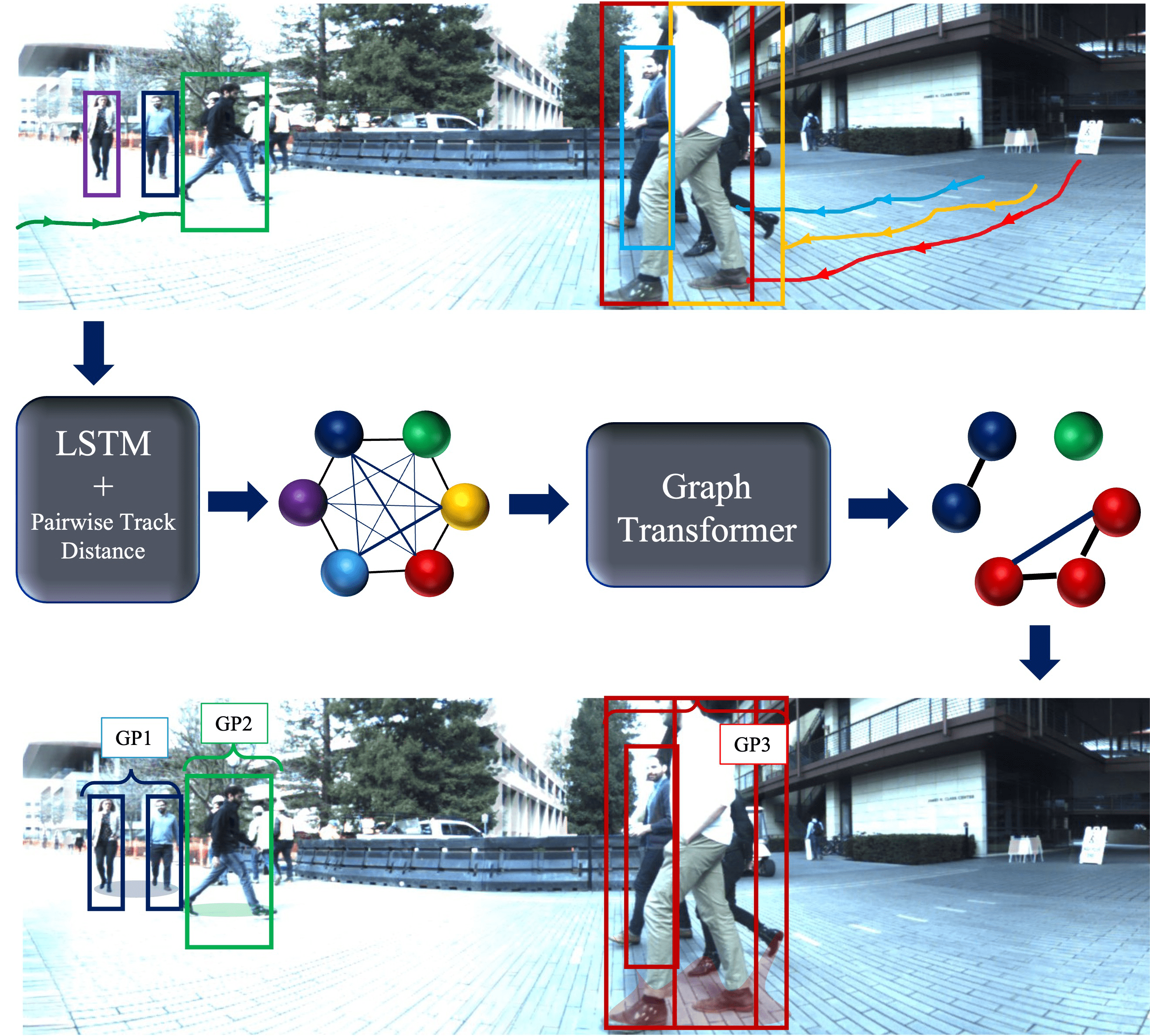
Figure 1: A schematic representation of our proposed framework. A set of tracks, represented as LSTM encoded features, serve as input to our model. Using a pairwise distance metric between these trajectories, a graph is constructed and fed into a graph transformer. The graph transformer clusters the nodes in the graph, ultimately allowing for the prediction of social groups.

Grouping individuals in a crowd presents a significant challenge due to the complexity and unpredictability of human social behavior. The major obstacle in group detection is encoding group characteristics with compact and meaningful features that can form well-defined clusters. To address this challenge, researchers have focused on grouping individuals based on their interactions [6, 7, 8], or by using F-formation techniques [9] to model group formations [10, 11]. Although these methods can effectively model group formations, they are limited to modelling only static groups [12]. Some efforts have been made to use trajectory information to detect groups based on similar temporal features [13, 14, 15, 16]. However, these methods often struggle in challenging scenarios due to their limited generalization capability [17]. With the advent of deep learning, recent approaches have relied on spatio-temporal representations using 3D neural networks such as I3D  [18, 19]. These methods combine visual and geometrical features to detect social groups. Additionally, a hierarchical graph neural network was proposed in [20] to model mutual social relations in a crowd of people. While these approaches have shown promising results, they are computationally expensive due to the dependency of their design in 3D neural networks, and, thus, may not be suitable for real-time applications in robotics. Recently [21] proposed to model multi-person behavior relationships by leveraging a self-supervised pre-training strategy and developing a self-attention network for group detection. This framework assumes that body pose and global position of all the individuals are available as inputs. Although the utilization of pose seems to be intuitive for better capturing human movements and interactions, in practice, the performance of the proposed method is susceptible to the pose estimation’ noise and errors. In fact, the inherent ambiguity of pose creates difficulties in interpretation, especially in scenarios where multiple individuals are in close proximity. In addition, this framework uses a two-stage training process. However, the effectiveness of the social relation embedding network in the first stage significantly impacts the performance of the second stage. In other words, any deficiencies in the first stage could carry over and adversely affect the model’s overall performance. This shortcoming is also validated by our experiments (Table  II).

We introduce a simple, swift and efficient framework to tackle the challenges involved in detecting social groups, as depicted in Fig.1. Our approach exclusively employs bounding boxes as input, which is less prone to noise than other inputs such as body pose. Furthermore, we make a deliberate effort to create a lightweight model by using LSTM and graph transformer techniques, resulting in a model with only 700K parameters and capable of real-time performance. We represent each individual as a node within a graph structure, deriving the node’s feature representation from encoding the subject’s trajectory and the bounding box coordinates over time, utilizing an LSTM. We calculate inter-subject distances, based on the methodology described in [22], and utilize them as edge features to serve as priors in the graph representation. We use a graph transformers to model the relationships between the nodes, where the node features encode the motion trajectory, and the edge features are based on the geometric distances between the subjects. The node features, updated through the graph transformer, are then combined with the geometric distances, and a multi-layer perception is employed to predict the number of social groups (cardinality) and track connectivity (adjacency matrix).
In this work, we present a novel and efficient deep architecture for detecting social groups. Our model has been evaluated on the large-scale and challenging JRDB dataset [19] and has achieved state-of-the-art performance. The inference time of our model is under 0.034 seconds, which is significantly faster compared to recent works [18, 19, 20], while utilizing the same computation resources. The key contributions of this work are as follows:

1. A novel and computationally efficient neural architecture is proposed, which uses a combination of LSTM and a graph transformer, and only requires the subjects’ trajectories as inputs.

2. A novel graph modeling approach is presented, where the motion of each trajectory is encoded as node features and the geometric distance between tracks is used as edge features.

3. Our model surpasses the performance of recent works and achieves a speed-up by up to 12 times.

II Related works

Social groups can be defined as emergent entities that are formed from the interactions and associations among two or more individuals who exhibit similar characteristics and exhibit a shared sense of unity. The automated detection of social groups is a topic of growing significance in the field of robotics, as it holds great promise for various applications, such as human-robot interaction, robot-assisted care, and social robot navigation. In this section, we present a concise overview of the recent developments in the research of social group detection.
F-formation technique: This technique is a method that has been employed by several studies for modelling the spatial structure in social groups. Cristani et al. [23] utilized statistical analysis to detect social interactions based on the spatial-orientational arrangements that are sociologically relevant. On the other hand, Setti et al. [11] utilized an efficient graph-cut based optimization to update the centers of the F-formations and prune unsupported groups using the Minimum Description Length principle. Despite its potential, the F-formation technique has certain limitations, as it is only capable of modelling the spatial structural formation and is not well-suited for dynamic group analysis [12]. This highlights the need for more advanced techniques that can model the temporal evolution of social groups, taking into account the changes in both the spatial and behavioral aspects of the group members.
Trajectory-based: Some studies have employed a trajectory-based approach. Pang et al. [24] utilized a multivariate stochastic differential equation to model the position and velocity of individuals in real-time. Meanwhile, Atevet al. [13] developed a method for clustering vehicle trajectories based on the combination of two spectral clustering methods and a trajectory similarity measure based on the Hausdorff distance. Solera et al. [14] proposed a tracklet clustering approach that utilized a defined distance function and four features to identify both the physical and social identity of pedestrians and to determine the presence of a shared goal. Chen et al. [15] introduced an Anchor-based Manifold Ranking (AMR) approach to examine the topological relationship of individuals and the global consistency of crowds in dense environments, accurately recognizing groups through a coherent merging strategy. Ayazoglu et al. [16] tackled the problem of casual interaction detection using a directed graph topology and modelled casual connections between trajectories using Granger Causality theory. However, despite these efforts, current approaches are insufficient for identifying groups in dense crowds. A recent study [21] presented a new framework for human group detection that uses human body pose trajectories as inputs and utilizes a two-stage multi-head approach, leveraging self-supervised social relation feature embedding and a self-attention inspired network. In this study, the use of human body pose estimation can enhance the recognition of human movement and interaction. However, it is important to note that estimation errors and noise can negatively impact the performance of the method.
Visual-content based approaches: In recent years, researchers have attempted to extract group-related information from visual images. Das et al. proposed the framework named Group-Sense, which identifies interacting groups based on acoustic context [25]. Another study combined orientation and context similarity in a parameter-free framework to cluster feature points [26] . Xie et al. modeled the interaction between individuals using a causality-induced hierarchical Bayesian model, where Granger causality was characterized by multiple features [12]. Li et al. proposed a method that profiles group properties using crowd trajectories and semantic information, then models multi-feature consistency and inconsistency in a unified graph clustering technique [17]. Ehsanpour et al. and Han et al. utilized an I3D feature extractor, a self-attention module, and a graph attention module, where each individual’s social interactions are encoded in a spatio-temporal feature map. Their model recognizes individuals’ actions and social activities of each social group, relying on other tasks such as individual action and social group activity detection using visual features [18, 19, 20]. The disadvantage of these visual-content based methods is that they require large-sized networks, such as I3D, for feature extraction, hindering their real-time applicability. To address these challenges and limitations, a more efficient method for robust social group detection in dynamic human environments is proposed.

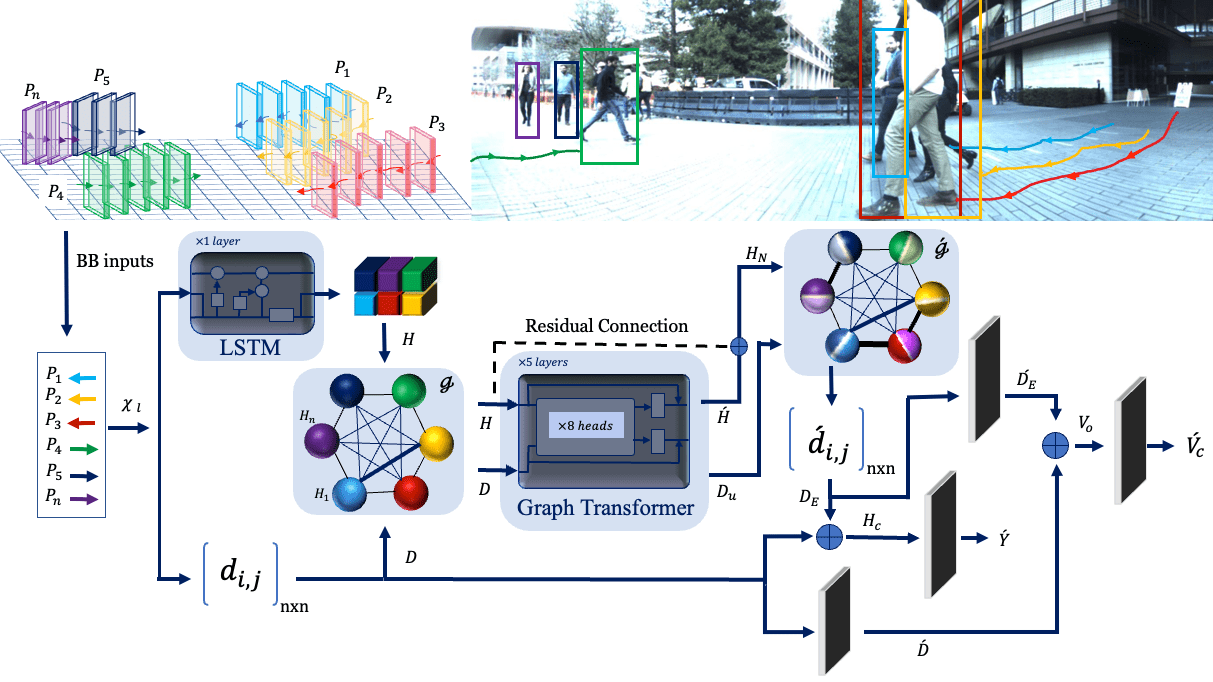
Figure 2: The overall pipeline of the proposed model consists of an LSTM encoder and a distance calculation module running in parallel, where $H$ and $D$ represent the node and edge of a graph, respectively. The generated graph is then processed by a modified graph transform module to update the node ($H_{N}$) and edge ($D_{u}$) features. The Euclidean distance between $H_{N}$ is calculated, concatenated with $D$, and fed into MLP layers to produce the adjacency matrix ($\acute{Y}$) and the number of groups ($\acute{V}_{c}$).

III Proposed Method

The crucial aspect of social group detection lies in encoding a robust joint spatiotemporal feature representation that encompasses the movements and interactions of all individuals within a group. To accomplish this, our proposed method employs the use of Long Short-Term Memory (LSTM) to encode the individual’s trajectories. We then merge the encoded trajectories with a graph transformer to obtain a model with 700k parameters, a significant reduction compared to existing models. This approach leverages the notion that members within a group tend to exhibit similar behaviors and trajectories and combines this information with the inter-track distances to form a graph. The graph transformer learns a joint representation of this graph, which is then clustered into several connected components via graph clustering and spectral clustering to identify social groups. Fig.2 outlines the framework of our method, and the paper provides a comprehensive elaboration of its details. For the reader’s ease of reference, Table  I summarizes the notations and symbols used throughout the paper.

Notations	Descriptions
$\mathcal{X}_{\ell}$	a set of different variable-length tracks
${Y}_{{\ell}}$	adjacency matrix between the tracks
$P_{i}$	$i_{th}$ instance track
$P^{t_{0}:t_{T}}_{i}$	sequence of i-th instance bounding boxes (track) over time span $t_{0}$-$t_{T}$
$B=F^{C}(A;\Theta)$	function named C with A as input, B as output and $\Theta$ as its parameter
$d^{GIoU}_{i,j}$	a normalized GIoU distance between $i_{th}$ and $j_{th}$ instance
$\tilde{d}_{0}(\{P^{t}_{i}\},\{P^{t}_{j}\})$	distance between $i_{th}$ and $j_{th}$ instance
$D_{P_{i}}$	time duration when the tracks $i$ exist
$\bm{d}_{i,j}(P_{i},P_{j})$	distance between two variable-length trajectories, $P_{i}$ and $P_{j}$
$\bigwedge$ , $\bigoplus$	logical operations functions
$\mathbin{\|}$	concatenation

TABLE I: Summary of Notation

Input and Output: We train our model using a training set with $L$ samples, i.e. $\{\mathcal{X}_{\ell},{Y}_{{\ell}}\}_{1}^{L}$, where the input, $\mathcal{X}_{\ell}=\{P_{1},P_{2},...,P_{n}\}$ is a set of different variable-length tracks (each track represents a single instance and consists of a sequence of bounding boxes). The output ${Y}_{{\ell}}=\bigg{[}y_{i,j}\bigg{]}_{n\times n}\in\mathbb{B}^{n\times n},y_{i,j}\in\{0,1\}$, represents the adjacency matrix between the tracks. The value $y_{i,j}$ indicates if two track instances belong to the same group ($y_{i,j}=1$) or not $(y_{i,j}=0)$.
The number of tracks is indicated by $n$ and $P^{t_{0}:t_{T}}_{i}$ represents a track for instance $i$, which is a sequence of its track states, $P^{t_{0}:t_{T}}_{i}=(\mathrm{p}^{t_{0}}_{i},\cdots,\mathrm{p}^{t_{T}}_{i})$, e.g. bounding box coordinates and sizes, within the time range from $t_{0}$ to $t_{T}$.
Spatio-Temporal Encoding: Each sequence of bounding boxes, $P^{t_{0}:t_{T}}_{i}$, is input to an LSTM module to extract the spatiotemporal characteristics of each instance’s trajectory motion, as described by Eq. (1).

$$H_{i}=F^{LSTM}(P^{t_{0}:t_{T}}_{i};\Theta_{1}),$$ (1)

where $F^{LSTM}(\cdot;\Theta_{1})$ is LSTM module that gets sequences of bounding boxes of a track and extracts its motion features and $H_{i}\in\mathbb{R}^{1\times N}$ indicates the encoded spatio-temporal feature vector for track $i$ as the output.
Calculating a Distance Between Two Variable-length Tracks: To determine a distance between two dynamic trajectories, $P_{i}$ and $P_{j}$, the time-averaged distance from OSPA⁽²⁾ (an extension of Optimal Sub-Pattern Assignment (OSPA)) [27] is utilized:

$$\bm{d}_{i,j}(P_{i},P_{j})=\sum_{t\in P_{i}\cup P_{j}}\frac{\tilde{d}_{0}(\{P_{i}^{t}\},\{P_{j}^{t}\})}{|D_{P_{i}}\cup D_{P_{j}}|},$$ (2)

where $D_{P_{i}}$ and $D_{P_{j}}$ represent the time duration when tracks $i$ and $j$ exist, respectively. When at least one of the tracks $i$ and $j$ exists, the time duration is represented by $D_{P_{i}}\cup D_{P_{j}}\neq\emptyset$. The value of $\bm{d}_{i,j}(P_{i},P_{j})$ is 0 if the time duration when the tracks $i$ and $j$ exist is an empty set, i.e., $D_{P_{i}}\cup D_{P_{j}}=\emptyset$.
Additionally, $\tilde{d}_{0}(\{P^{t}_{i}\},\{P^{t}_{j}\})$ calculates the distance between two Singleton sets, and is determined using equations inspired by the OSPA set distance formula  [28]  [29] :

$$\tilde{d}_{0}(\{P^{t}_{i}\},\{P^{t}_{j}\})=\begin{cases}d^{GIoU}_{i,j}&\text{if $|\{P^{t}_{i}\}|\wedge|\{P^{t}_{j}\}|=1$},\\ 1&\text{if $|\{P^{t}_{i}\}|\oplus|\{P^{t}_{j}\}|=1$},\\ 0&\text{Otherwise},\end{cases}$$ (3)

where $d^{GIoU}_{i,j}=\frac{1-GIoU(i,j)}{2}$ is used to calculate the normalized GIoU distance between tracks $i$ and $j$, with a range of values between 0 and 1, when both tracks exist at time $t$, i.e. $|\{P^{t}_{i}\}|\wedge|\{P^{t}_{j}\}|=1$. If at least one instance does not exist (Second term) i.e., $|\{P^{t}_{i}\}|\oplus|\{P^{t}_{i}\}|=1$ , the distance is set to the maximum value of 1. Otherwise, the distance is 0, as shown in third term. The calculation process is demonstrated in Fig. 3.

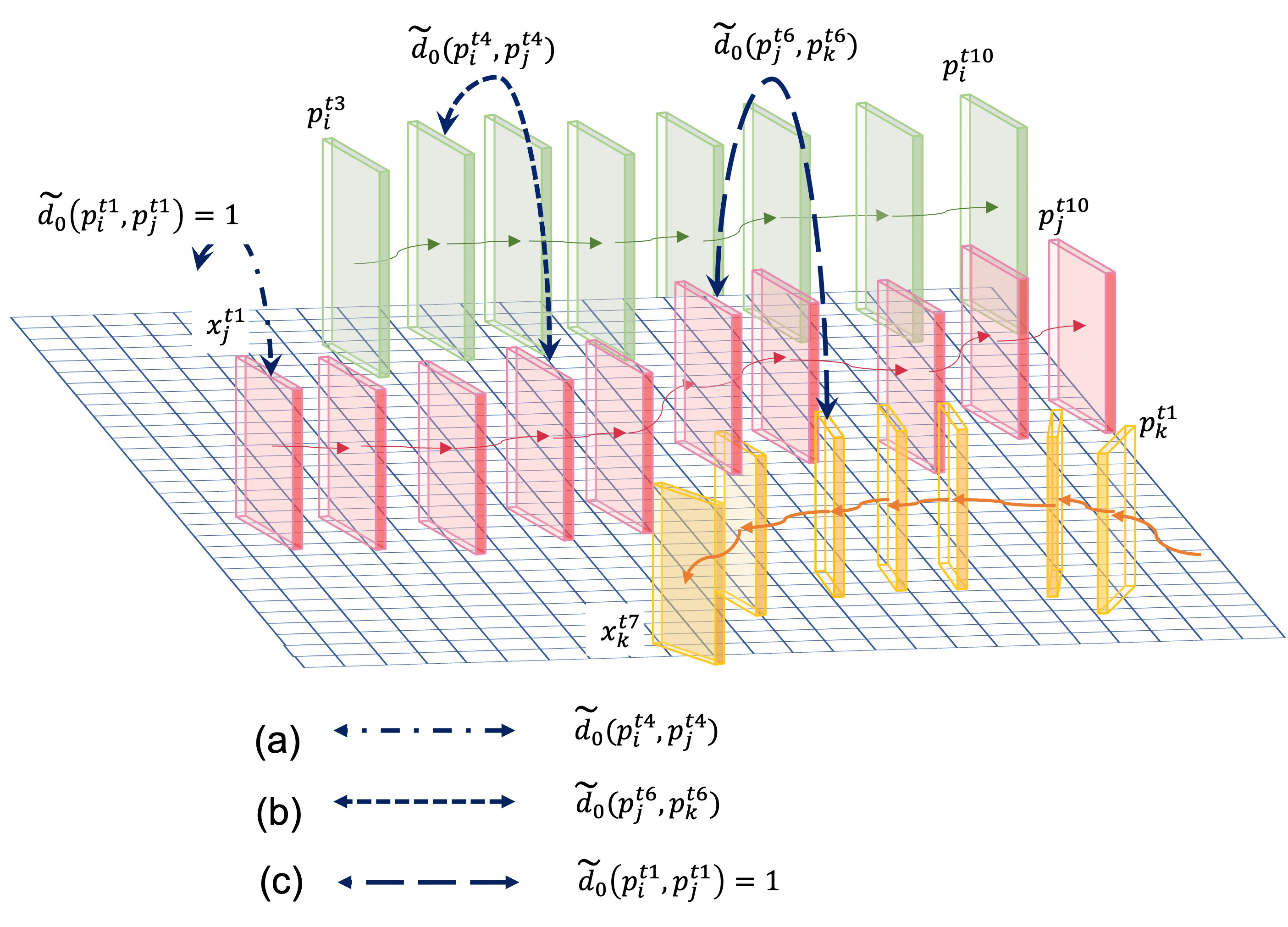
Figure 3: Distance calculation among motion trajectories using GIoU metric based on Eq.(3). The scenarios depicted in (a) and (b) represent instances where both instances are present, while scenario (c) represents a situation where one of the instances is absent in the frame.

Modeling Graph: The graph $\mathcal{G}=\{H,D\}$ models the relationship between tracks (instances). The set $H$ contains nodes that represent the spatiotemporal features of each track (encoded by an LSTM), while the set $D$ consists of edges that denote the distances between tracks, defined above. The graph transformer, as described in [30], is employed to modify and enhance the features of both nodes and edges.

$$\acute{\mathcal{G}}=F^{GR}(\mathcal{G};\Theta_{2}),$$ (4)

Where $F^{GR}(\cdot;\Theta_{2})$ is graph transformer module that processes generated graph, $\mathcal{G}=\{H,D\}$, and produces updated graph $\acute{\mathcal{G}}=\{H_{N},D_{u}\}$, $H_{N}$ denoted the updated node features that defined as $H_{N}=H+\acute{H}$ and $\acute{H}$ shows the residual connection, illustrated in Fig. 2. Also, $D_{u}$ is updated edge features.
Then the Euclidean distance, $D_{E}$, between each node feature, $H_{N}$, has been calculated and concatenated with the distance between tracks.

$$D_{E}=\Bigr{[}\acute{d}_{i,j}\Bigr{]}_{n\times n}\in\mathbb{R},\acute{d}_{i,j}\in[\ 0-1],$$ (5)

$$H_{c}=D_{E}\mathbin{\|}D,$$ (6)

where $\mathbin{\|}$ means concatenation. Finally, a simple module that consists of MLPs (Multi-Layer Perceptrons) is utilized to predict the adjacency matrix, $\acute{Y}$.

$$\acute{Y}=F^{L_{1}}(H_{c};\Theta_{3}).$$ (7)

$F^{L_{1}}(\cdot;\Theta_{3})$ is an MLP layer, $D_{E}$ and $D$ are passed through few MLP layers $\acute{D}_{E}=F^{L_{2}}(H_{N};\Theta_{4})$ and $\acute{D}=F^{L_{3}}(D;\Theta_{5})$ then after concatenation ${V}_{o}=\acute{D}_{E}\mathbin{\|}\acute{D}$ feeds to a final linear layer to predict the number of social groups (cardinality), $\acute{V}_{c}$, i.e.,

$$\acute{V}_{c}=F^{L_{4}}({V}_{o};\Theta_{6}),$$ (8)

where $F^{L_{4}}(\cdot;\Theta_{6})$ is an MLP layer, given concatenated vector ${V}_{o}$ and produces $\acute{V}_{c}$ which shows number of groups.
Loss Function: We used the loss function same as [19], the loss is combination of three losses: $\mathcal{L}_{BCE}$, $\mathcal{L}_{eig}$ and $\mathcal{L}_{MSE}$, shown in Eq. (9).

$$\mathcal{L}_{G}=\lambda_{1}\mathcal{L}_{BCE}(\acute{Y},Y)\!+\!\lambda_{2}\mathcal{L}_{eig}(\acute{L},L)\!+\!\lambda_{3}\mathcal{L}_{MSE}(\acute{V}_{c},V_{c}),$$ (9)

where $\lambda_{1}$, $\lambda_{2}$ and $\lambda_{3}$ are the coefficient weights of the loss terms. The variables with $\acute{(.)}$ denote the corresponding ground-truth labels.
A binary cross-entropy loss, $\mathcal{L}_{BCE}$, is used between the elements of predicted adjacency, $\acute{Y}$, and ground truth adjacency, $Y$. We also utilize $\mathcal{L}_{eig}$ denoted by Eq. (10) and is inspired by the fully differentiable, eigen decomposition-free loss proposed in [31] to train a deep network whose loss depends on the eigenvector of the matrix predicted by the network containing a single zero eigenvalue. The number of social groups (connected components) in ground truth matrix $Y$ corresponds to the number of zero eigenvalues of its laplacian matrix $L$, we calculate the laplacin matrix of $\acute{Y}$ noted by $\acute{L}$ to achieve zero eigenvalues, same as in $L$. To this end, Eq. (10) is utilized below.

$$L_{eig}=e^{T}\acute{L}^{T}\acute{L}e+\alpha\exp(-\beta tr(\bar{\acute{L}}^{T}\bar{\acute{L}})),$$ (10)

with $e$ as the ground truth eigenvector corresponding to zero eigenvalue, the laplacian matrix $\acute{L}$ corresponds to the predicted similarity matrix $\acute{Y}$, while $\alpha$ and $\beta$ are coefficients. More details and the proof of Eq. (10) is stated in [19].
Finally, $\mathcal{L}_{MSE}$ is a mean square error (cardinality loss), which is used to predict the number of social groups (number of connected components).

Training: Considering the compounded parameters of the suggested neural models as $\mathbf{\Theta}=(\Theta_{1},\Theta_{2},\dots,\Theta_{6})$, we train them end-to-end by minimizing the total loss over $\mathbf{\Theta}$, i.e. $\mathbf{\Theta}^{*}=\arg\min_{\mathbf{\Theta}}\sum_{\ell=1}^{L}\mathcal{L}^{\ell}_{G}$, using stochastic gradient descent [32].
Inference: We use graph spectral clustering [33] on the predicted adjacency matrix, $\acute{Y}$, and the predicted number of social groups, $\acute{V}_{c}$, to detect the social groups. Spectral clustering employs the heuristic [34] to determine the number of social groups present.

IV Experiments

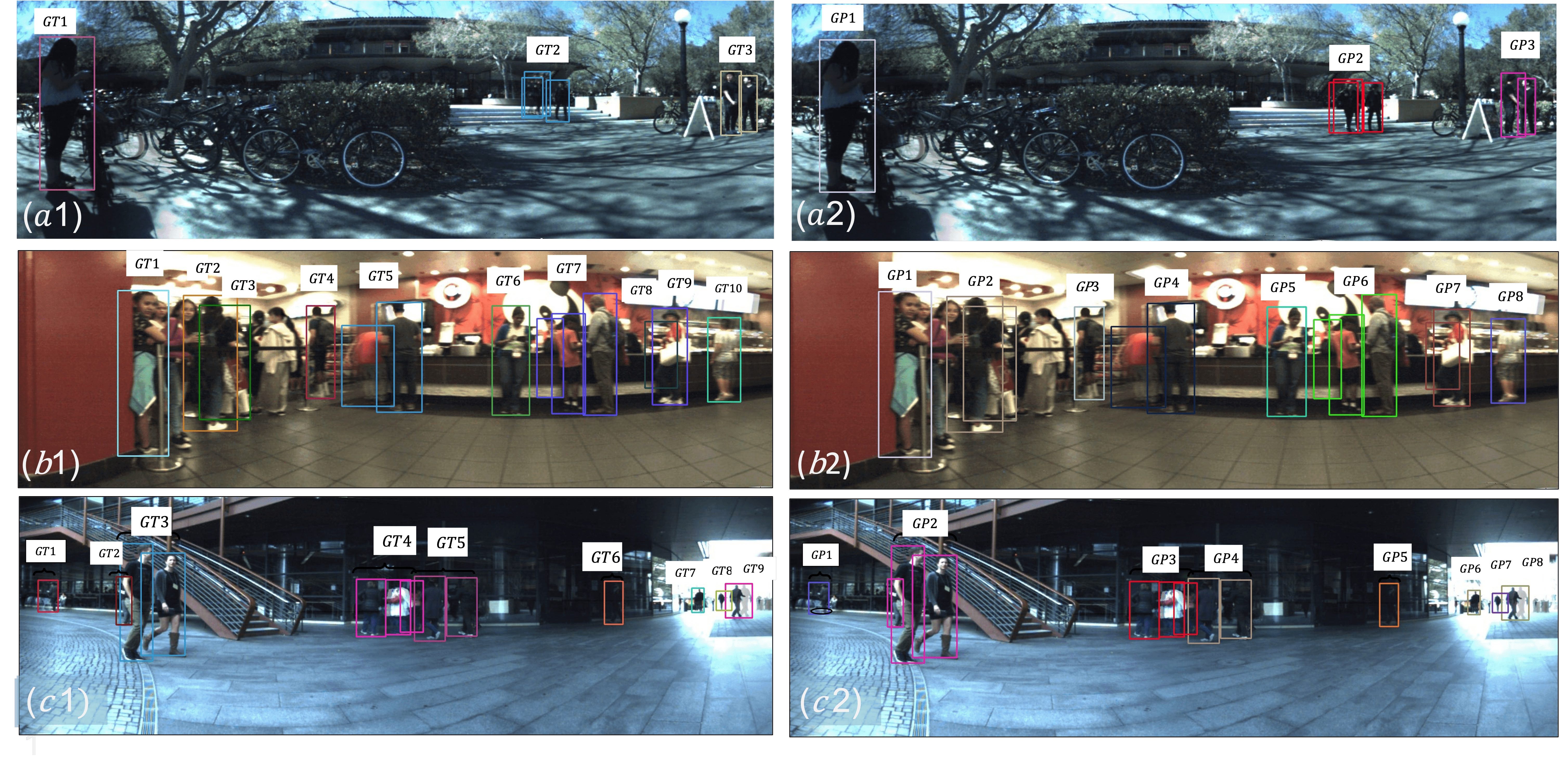
Figure 4: The visualization of our model’s performance on the validation set is depicted in $(a1),(b1)$, and $(c1)$, which represent the ground truth, while $(a2),(b2)$, and $(c2)$ depict the groups detected by our model. Our model demonstrates exceptional results in both straightforward $(a2)$ and complex $(b2)$ and $(c2)$ scenes. However, there is still scope for improvement. For instance, in $(b2)$, the group ”GP2” is not fully associated with the ground truth groups ”GT2” and ”GT3” in $(b1)$.

Set	Method	G1 AP$\uparrow$	G2 AP$\uparrow$	G3 AP$\uparrow$	G4 AP$\uparrow$	G5+ AP$\uparrow$	mAP$\uparrow$
	Li et al. [21]	3.1	25.0	17.5	45.6	25.2	23.3
	Ehsanpour et al. [18]	8.0	29.3	37.5	65.4	67.0	41.4
Validation	Han et al. [20]	52.0	59.2	46.7	46.6	31.1	47.1
	Ehsanpour et al. [19]	81.4	64.8	49.1	63.2	37.2	59.2
	Ours	71.9	73.6	64.0	71.2	48.6	65.9
	Ehsanpour et al. [18]	11.2	24.6	21.8	41.2	23.5	24.5
Test	Ehsanpour et al. [19]	56.3	39.4	24.3	22.9	15.3	31.6
	Ours	19.5	39.7	30	48.6	24.7	32.5

TABLE II: Social Group Detection on JRDB-Act (Validation/Test)-Set using the ground truth detection/tracks.

Method	Num. Parameters$\downarrow$	fps$\uparrow$
Ehsanpour et al. [18]	27M+	2.40-
Ehsanpour et al. [19]	27M	2.40
Han et al. [20]	23M+	2.3-
Li et al. [21]	1.6M	29.41-
Ours	700K	29.41

TABLE III: Comparison Between Number of Parameters and Inference FPS. ”⁺” and ”^-” indicate a greater and a lower values, respectively.

Dataset: Our model is tested on the demanding JRDB-Act dataset [19], which captures dynamic social interactions in crowded indoor and outdoor environments on the Stanford University campus. Social group annotations are determined based on the behavior and activities of individuals within the scene. Adhering to the JRDB-Act protocol, the effectiveness of our model’s social group detection capabilities is evaluated on key frames selected every 15 frames from the dataset. The dataset comprises a total of 1419 training samples, 404 validation samples, and 1802 testing samples.
Evaluation Metric: We employ the mean Average Precision (mAP) metric, introduced in [19], which calculates the Average Precision (AP) for various group sizes ranging from one to more than five members indicated by G1 (one member), G2 (two members), and G5+ (more than five members) in Table II. The evaluation for each task is conducted using the corresponding ground truth labels, consistent with the methodology outlined in [19].
Implementation Details: The proposed method employs a sequence of bounding boxes, consisting of a maximum of 15 frames selected from 30 frames prior to the key-frame by choosing every other frame. The frames are then fed to LSTM module with a feature dimension of 32. The graph transformer component of the model is comprised of 5 layers with 8 attention heads.

The function $F^{L_{1}}$, as defined in Eq. (7), is a (2$\times$1) multi-layer perceptron (MLP) layer with a sigmoid activation function. The functions $F^{L_{2}}$ and $F^{L_{3}}$, defined in the equations, are MLP layers with dimensions (32$\times$16) and (1$\times$16), respectively, and utilize a ReLU activation function. The function $F^{L_{4}}$, defined in Eq. (2), is a (32$\times$1) linear layer.

The optimization process is performed using the ADAM optimizer with hyperparameters $\eta_{1}=0.9$, $\eta_{2}=0.999$, and $\epsilon=10^{-8}$. The parameters in Eq.( 9) are set to $\lambda_{1}=5\times 10^{-4}$, $\lambda_{2}=0.1$ and $\lambda_{3}=5\times 10^{-4}$ and $\alpha$ and $\beta$ in Eq. (10) are both equal to 1. The model is trained for 50 epochs using a mini-batch size of 1 and an initial learning rate of $10^{-4}$, which is reduced by a factor of $0.1$ if the validation loss plateaus.

The experiment is conducted on an NVIDIA GeForce GTX 1080 Ti and a comparison is made with previous state-of-the-art frameworks [18, 19, 20] in terms of inference time. For a fair comparison, only the feed-forward time of each neural architecture is reported in the results.

Model	Det/Track	$D_{E}$	GAT/G.Trans	Res Co	G1 AP$\uparrow$	G2 AP$\uparrow$	G3 AP$\uparrow$	G4 AP$\uparrow$	G5+ AP$\uparrow$	mAP$\uparrow$
GAT/Graph Transformer	Track	✓	GAT	✓	46.8	67.6	74.0	71.2	50.6	62.0
w/o Euclidean Distance	Track	✗	G.Trans	✓	72.7	71	62.2	65.7	44.2	63.2
w/o Motion Trajectory	Det	✓	G.Trans	✓	63.1	65.7	63.6	76.9	55	64.8
w/o Residual Connection	Track	✓	G.Trans	✗	68.5	68.9	61.7	73.6	52.1	64.9
Our Final Model	Track	✓	G.Trans	✓	71.9	73.6	64.0	71.2	48.6	65.9

TABLE IV: An ablation study on JRDB-Act validation-set using the ground truth Detection/Tracks.

IV-A Results

Table II displays a comparison between our model and the other state-of-the-art methods on the both validation and test JRDB-Act data. Our proposed method has achieved considerable performance improvement compared to the state-of-the-art approaches, i.e. [19], [20], [18], and [21], in the both validation and test data. Moreover, our approach attained either the highest or second-highest AP scores across various group size categories in both the validation and test data. However, our method did not perform well in identifying one-member groups (G1) due to the difficulty in detecting individuals in crowded scenes where they are in close proximity to one another. In such situations, distance-based techniques may not provide accurate results.
One of the main reasons for the success of our approach is its reliance on simple and efficient input data (bounding boxes) along with the encoding of each individual’s trajectory over time. This approach is less prone to noise compared to the other competitive methods using more complex input data, e.g. video or body pose, while offering significant computational efficiency compared to them. Furthermore, we employ a graph transformer to model the relationships between nodes, which may prove more effective. By incorporating trajectory information into node features and geometric distances between subjects in edge features, we can achieve more accurate modelling of social relations. Moreover, in our approach, the distances between trajectories are employed as edge features to serve as priors in the graph representation, which differs from the approach taken by [18] and [19] where the graph is fully connected as an input to the GAT.
Note that, all the methods reported in Table II used ground truth bounding boxes for reporting their results on the validation set. However, since no ground-truth bounding box was available for the test data, the performance of all the methods on this set relied on the detections/tracks generated by [35]. Although its detection performance is reasonable (i.e. AP0.5 = 68.1%), its tracking performance is not as well as its detection and is moderately low, (i.e. MOTA = 32.3%). We anticipated this reduction in performance for test data and believe that a better tracking algorithm could further improve our method’s results. It is important to mention that we have presented results for [18] and [19], while the test results for [20] and [21] were unavailable.
Table III displays the number of parameters used by each model (Num. Parameters) and its processing speed, represented in frames per second (fps). In terms of the number of parameters, model [21] has a relatively small number of parameters (1.6 million), while models [18, 19], and [20] have significantly larger numbers of parameters, at 27 million, over 27 million (indicated by 27M⁺), and 23 million, respectively. This increase in parameters is due to the use of modules such as I3D, RoiAlign, and GAT. Our method, which has 700,000 parameters and LSTM and graph transformer as its main modules, represents a trade-off between model complexity, capacity to learn from data, and computational efficiency. In terms of computational cost (fps), model [21] has a fps rate of less than 29.41 (indicated by 29.41^-) due to its number of parameters. Models [18, 19] have lower fps rates of less than 2.40 and 2.3, respectively, due to their high number of parameters. Model [20] also has a low fps rate of less than 2.3 due to its use of the same backbone as [18, 19] and GCN modules. Our method, with 700,000 parameters and LSTM and graph transformer as its main modules, has a fps rate of 29.41, which is the best, highlighting the trade-off between model complexity, capacity to learn from data, and computational efficiency.

Qualitative Results: We visualize the detected groups in selected images from the validation set in Fig. 4. In each pair, images on the left show the ground truth $(a1)$, $(b1)$ and $(c1)$, while the images on the right illustrate the output of our model $(a2)$, $(b2)$ and $(c2)$. From the comparison, we can observe that our model performs well not only in simple scenes such as $(a2)$ but also in challenging scenes such as $(b2)$. In $(a2)$, GP1, GP2, and GP3 are evidence of our model’s excellent performance, corresponding to GT1, GT2, and GT3 in the ground truth image $(a1)$, respectively. However, our model still faces difficulties in detecting challenging groups where individuals are far apart in depth but close in x, y coordinates. For instance, in the ground truth image $(b1)$, GT2 and GT3 are separate groups, but they are considered as one group, GP2, in $(b2)$. Similarly, in $(c1)$, we can see that GT2 and GT3 are separated, but our model detects them as one group, GP2. This issue arises when, in some scenes, the trajectory of each individual is not well encoded and the distance calculation technique considers them as a group. To overcome this limitation, incorporating more information and encoding a richer feature representation could be beneficial in detecting interacting people in social groups. For example, considering interaction, body pose, and head orientation in addition to calculating distances could greatly enhance the social group detection capabilities of our model.

IV-B Ablation Study

The efficacy of each constituent element in our proposed methodology is demonstrated through a comprehensive ablation analysis in Table  IV. The final performance on the JRDB-Act validation set is evaluated by systematically removing each essential component, allowing us to assess their individual impact on the final performance. These experiments are conducted using ground truth bounding boxes from the validation set to eliminate the influence of detection performance. One key element of the ablation is the evaluation of the graph transformer, as depicted in Fig.2. To evaluate its effectiveness, the GAT model [36] is adopted instead of the graph transformer (G.Trans), as indicated by the ”GAT/G.Trans” entry in Table  IV. Additionally, the Euclidean distance ($D_{E}$) as defined in Eq. (5) is used to calculate the distance between the updated node features ($H_{N}$). The role of trajectory is also explored, as depicted by the ”Det/Track”. The ”Det” notation indicates that only a single key-frame is considered, with no trajectory information provided to the LSTM module, while the ”Track” notation indicates that 15 frames are considered, allowing us to calculate the distance between trajectories as described in Sec.III ”Calculating a Distance Between Two Variable-sized Tracks”. Lastly, the residual connection depicted in Fig.2, which connects the input of the graph transformer to its output, is evaluated and referred to as ”Res Co” in Table  IV. Further details regarding each ablation can be found in the following:

GAT vs Graph Transformer: In this ablation study, the GAT model is compared against the graph transformer. The other components are kept unchanged. As displayed in Table IV, the results show that the performance decreases by 5.9% mAP when using the GAT model instead of the graph transformer. This disparity can be attributed to the multi-headed attention mechanism employed by the graph transformer, which significantly improves attention compared to the GAT model. Furthermore, as demonstrated in [30], the generalization performance of transformer networks to graph data is significantly higher than that of GAT models. With vs Without Euclidean Distance: In this ablation, the contribution of the Euclidean distance ($D_{E}$) is evaluated. The $D_{E}$, which calculates the Euclidean distance between the updated node features, is removed, and instead, the $H_{N}$ is concatenated with D as described in Eq.(6). This change transforms Eq.(6) into $H_{c}=H_{N}\mathbin{\|}D$. The Euclidean distance between the encoded motion trajectory, updated by the graph transformer, is combined with the pairwise track distance, contributing to a more effective encoding of the distance between individuals in a group. Table IV shows a 4% decrease in mAP.
With vs Without Motion Trajectory: This ablation study evaluates the impact of removing the motion trajectory of individuals in our model. The 15 frames are eliminated, and only the last frame is used to calculate the distance, ${d}_{i,j}$. As a result, instead of calculating the distance between two trajectories, $\bm{d}_{i,j}(P_{i},P_{j})$, the distance between two bounding boxes is calculated. Consequently, only one frame is fed into the LSTM, while the rest of the model remains unchanged. The results show that considering the motion trajectory improves the performance by 1.69% in terms of mAP.
With vs Without Residual Connection: The architecture of our proposed method, as shown in Fig. 2, includes a residual connection that connects the input of the graph transformer to its output. This ablation study aims to verify the role of the residual connection in our model by removing it. The results, shown in Table IV, indicate that the residual connection outperforms the model without it by a margin of 1.5%. It is believed that the residual connection helps the graph transformer to more efficiently learn the distance between instances, thus allowing the model to learn better.

V CONCLUSIONS

In this paper, we present a simple, but efficient, end-to-end supervised model that represents the first graph transformer-based approach in the field of social group detection. Our solution stands out in its ability to use only the coordinates of bounding boxes as the input to the model, while simultaneously achieving faster performance than previous state-of-the-art models. We model the social group detection problem as a graph, with the node features estimated by encoding tracks using LSTM and the edge values determined by the time-average distance between each track pair. Our model achieves state-of-the-art results on the JRDB-Act benchmark dataset and outperforms previous methods in terms of both performance and speed. In future, we aim to enrich the input feature representation for this task by incorporating additional information such as individuals’ actions, body poses, and head orientations. This will lead to an even richer and more comprehensive representation of the social group dynamics.

References

- [1] T. Kruse, A. K. Pandey, R. Alami, A. Kirsch, Human-aware robot navigation: A survey, Robotics and Autonomous Systems 61 (12) (2013) 1726–1743.
- [2] A. Kubota, T. Iqbal, J. A. Shah, L. D. Riek, Activity recognition in manufacturing: The roles of motion capture and semg+ inertial wearables in detecting fine vs. gross motion, in: 2019 International Conference on Robotics and Automation (ICRA), IEEE, 2019, pp. 6533–6539.
- [3] M. Hanheide, D. Hebesberger, T. Krajník, The when, where, and how: An adaptive robotic info-terminal for care home residents, in: Proceedings of the 2017 ACM/IEEE International Conference on Human-Robot Interaction, 2017, pp. 341–349.
- [4] H. B. Barua, C. Sarkar, A. A. Kumar, A. Pal, et al., I can attend a meeting too! towards a human-like telepresence avatar robot to attend meeting on your behalf, arXiv preprint arXiv:2006.15647 (2020).
- [5] F. Caba Heilbron, V. Escorcia, B. Ghanem, J. Carlos Niebles, Activitynet: A large-scale video benchmark for human activity understanding, in: Proceedings of the ieee conference on computer vision and pattern recognition, 2015, pp. 961–970.
- [6] W. Choi, Y.-W. Chao, C. Pantofaru, S. Savarese, Discovering groups of people in images, in: European conference on computer vision, Springer, 2014, pp. 417–433.
- [7] W. Ge, R. T. Collins, R. B. Ruback, Vision-based analysis of small groups in pedestrian crowds, IEEE transactions on pattern analysis and machine intelligence 34 (5) (2012) 1003–1016.
- [8] H. Hung, B. Kröse, Detecting f-formations as dominant sets, in: Proceedings of the 13th international conference on multimodal interfaces, 2011, pp. 231–238.
- [9] A. Kendon, Conducting interaction: Patterns of behavior in focused encounters, Vol. 7, CUP Archive, 1990.
- [10] H. B. Barua, P. Pramanick, C. Sarkar, T. H. Mg, Let me join you! real-time f-formation recognition by a socially aware robot, in: 2020 29th IEEE International Conference on Robot and Human Interactive Communication (RO-MAN), IEEE, 2020, pp. 371–377.
- [11] F. Setti, C. Russell, C. Bassetti, M. Cristani, F-formation detection: Individuating free-standing conversational groups in images, PloS one 10 (5) (2015) e0123783.
- [12] Z. Xie, T. Wu, X. Yang, L. Zhang, K. Wu, Jointly social grouping and identification in visual dynamics with causality-induced hierarchical bayesian model, Journal of Visual Communication and Image Representation 59 (2019) 62–75.
- [13] S. Atev, G. Miller, N. P. Papanikolopoulos, Clustering of vehicle trajectories, IEEE transactions on intelligent transportation systems 11 (3) (2010) 647–657.
- [14] F. Solera, S. Calderara, R. Cucchiara, Socially constrained structural learning for groups detection in crowd, IEEE transactions on pattern analysis and machine intelligence 38 (5) (2015) 995–1008.
- [15] M. Chen, Q. Wang, X. Li, Anchor-based group detection in crowd scenes, in: 2017 IEEE International Conference on Acoustics, Speech and Signal Processing (ICASSP), IEEE, 2017, pp. 1378–1382.
- [16] M. Ayazoglu, B. Yilmaz, M. Sznaier, O. Camps, Finding causal interactions in video sequences, in: Proceedings of the IEEE International Conference on Computer Vision, 2013, pp. 3575–3582.
- [17] M. Li, T. Chen, H. Du, N. Ma, X. Xi, Social group detection based on multi-level consistent behaviour characteristics, Transportmetrica A: Transport Science (2021) 1–18.
- [18] M. Ehsanpour, A. Abedin, F. Saleh, J. Shi, I. Reid, H. Rezatofighi, Joint learning of social groups, individuals action and sub-group activities in videos, in: European Conference on Computer Vision, Springer, 2020, pp. 177–195.
- [19] M. Ehsanpour, F. Saleh, S. Savarese, I. Reid, H. Rezatofighi, Jrdb-act: A large-scale dataset for spatio-temporal action, social group and activity detection, in: Proceedings of the IEEE/CVF Conference on Computer Vision and Pattern Recognition, 2022, pp. 20983–20992.
- [20] R. Han, H. Yan, J. Li, S. Wang, W. Feng, S. Wang, Panoramic human activity recognition, in: Computer Vision–ECCV 2022: 17th European Conference, Tel Aviv, Israel, October 23–27, 2022, Proceedings, Part IV, Springer, 2022, pp. 244–261.
- [21] J. Li, R. Han, H. Yan, Z. Qian, W. Feng, S. Wang, Self-supervised social relation representation for human group detection, in: Computer Vision–ECCV 2022: 17th European Conference, Tel Aviv, Israel, October 23–27, 2022, Proceedings, Part XXXV, Springer, 2022, pp. 142–159.
- [22] H. Rezatofighi, N. Tsoi, J. Gwak, A. Sadeghian, I. Reid, S. Savarese, Generalized intersection over union: A metric and a loss for bounding box regression, in: Proceedings of the IEEE/CVF conference on computer vision and pattern recognition, 2019, pp. 658–666.
- [23] M. Cristani, L. Bazzani, G. Paggetti, A. Fossati, D. Tosato, A. Del Bue, G. Menegaz, V. Murino, Social interaction discovery by statistical analysis of f-formations., in: BMVC, Vol. 2, Citeseer, 2011, pp. 10–5244.
- [24] S. K. Pang, J. Li, S. J. Godsill, Detection and tracking of coordinated groups, IEEE Transactions on Aerospace and Electronic Systems 47 (1) (2011) 472–502.
- [25] S. Das, S. Chatterjee, S. Chakraborty, B. Mitra, Groupsense: A lightweight framework for group identification, IEEE Transactions on Mobile Computing 18 (12) (2018) 2856–2870.
- [26] Q. Wang, M. Chen, F. Nie, X. Li, Detecting coherent groups in crowd scenes by multiview clustering, IEEE transactions on pattern analysis and machine intelligence 42 (1) (2018) 46–58.
- [27] M. Beard, B. T. Vo, B.-N. Vo, A solution for large-scale multi-object tracking, IEEE Transactions on Signal Processing 68 (2020) 2754–2769.
- [28] H. Rezatofighi, T. T. D. Nguyen, B.-N. Vo, B.-T. Vo, S. Savarese, I. Reid, How trustworthy are the existing performance evaluations for basic vision tasks?, arXiv preprint arXiv:2008.03533 (2020).
- [29] D. Schuhmacher, B.-T. Vo, B.-N. Vo, A consistent metric for performance evaluation of multi-object filters, IEEE transactions on signal processing 56 (8) (2008) 3447–3457.
- [30] V. P. Dwivedi, X. Bresson, A generalization of transformer networks to graphs, arXiv preprint arXiv:2012.09699 (2020).
- [31] Z. Dang, K. M. Yi, Y. Hu, F. Wang, P. Fua, M. Salzmann, Eigendecomposition-free training of deep networks with zero eigenvalue-based losses, in: Proceedings of the European Conference on Computer Vision (ECCV), 2018, pp. 768–783.
- [32] L. Bottou, Stochastic gradient descent tricks, in: Neural networks: Tricks of the trade, Springer, 2012, pp. 421–436.
- [33] L. Zelnik-Manor, P. Perona, Self-tuning spectral clustering, Advances in neural information processing systems 17 (2004).
- [34] A. Ng, M. Jordan, Y. Weiss, On spectral clustering: Analysis and an algorithm, Advances in neural information processing systems 14 (2001).
- [35] Y. He, W. Yu, J. Han, X. Wei, X. Hong, Y. Gong, Know your surroundings: Panoramic multi-object tracking by multimodality collaboration, in: Proceedings of the IEEE/CVF Conference on Computer Vision and Pattern Recognition, 2021, pp. 2969–2980.
- [36] P. Veličković, G. Cucurull, A. Casanova, A. Romero, P. Lio, Y. Bengio, Graph attention networks, arXiv preprint arXiv:1710.10903 (2017).