State Classification via a Random-Walk-Based Quantum Neural Network

Abstract

In quantum information technology, crucial information is regularly encoded in different quantum states. To extract information, the identification of one state from the others is inevitable. However, if the states are non-orthogonal and unknown, this task will become awesomely tricky, especially when our resources are also limited. Here, we introduce the quantum stochastic neural network (QSNN), and show its capability to accomplish the binary discrimination of quantum states. After a handful of optimizing iterations, the QSNN achieves a success probability close to the theoretical optimum, no matter whether the states are pure or mixed. Other than binary discrimination, the QSNN is also applied to classify an unknown set of states into two types: entangled ones and separable ones. After training with four samples, it can classify a number of states with acceptable accuracy. Our results suggest that the QSNN has the great potential to process unknown quantum states in quantum information.

Quantum state discrimination identifies a quantum state among an already known set of candidate states. It is a key step in many quantum technologies as quantum states are the carriers of information in quantum computing protocols and quantum information processing. Although quantum mechanics fundamentally forbids deterministic discrimination of non-orthogonal states, probabilistic methods such as the minimum error discrimination helstrom1969quantum and the unambiguous discrimination ivanovic1987differentiate ; dieks1988overlap ; peres1988differentiate , have been developed, and their theoretical best performances have also been found. Beyond state discrimination, a special case of classification, one would expect to classify quantum states by more properties in one’s own particular interests. A well studied example is the classification of states according to whether the state is entangled or not. Lots of strategies have been proposed for detecting entanglement, such as using the positive partial transpose (PPT) criterion horodecki1995violating , entanglement witnesses horodecki1996separability ; terhal2000bell ; lewenstein2000optimization , and the Clauser-Horne-Shimony-Holt (CHSH) inequality bell1964einstein ; clauser1969proposed .

Most of the strategies mentioned above require complete knowledge of the quantum states before carrying out their best practices. However, exactly determining all the states is in principle forbidden, unless infinite copies of the states are provided. In Ref. massar2005optimal , Massar and Popescu have addressed this topic, known as the state estimation, and proved that the optimal mean fidelity for two-level system state estimation is $\frac{N+1}{N+2}$, where $N$ is the number of identically prepared copies of the state. The optimal mean fidelity is less than $1$ and tends towards $1$ as the number of copies $N$ tends to infinity. Then, in Ref. bruss1999optimal the authors extended the result to finite dimensional quantum systems in pure states. All these results indicate that the pre-processing of quantum state estimation before carrying out the state discrimination or classification will introduce extra errors. In addition, state estimation often involves a quantum information technology called state tomography, which is sometimes prohibitively expensive to perform on an unknown state paris2004quantum . In the states classification task, it also becomes practically impossible to do a tomography for each state, because the number of states waiting to be classified can be extremely large. In addition to the extra errors introduced by the pre-processing and the expensive tomography, there is another difficulty for these traditional strategies. That is, even if we exactly know the quantum states to be identified or classified, the optimal measurement is hard to be analytically developed in the fashion of traditional strategies, when more than two states are involved bergou2010discrimination ; barnett2009quantum .

Facing the above difficulties, we hope there will be a new strategy for state discrimination and classification. Recently, there has been a rising trend of using machine learning methods to fully exploit the inherent advantages of quantum technologies sarma2019machine ; carleo2019machine . Among these studies, the classification problem has received a great deal of attention, and some quantum classifiers have shown excellent performance schuld2020circuit ; li2022recent . In addition, as a fusion of deep learning and quantum computation, quantum neural networks biamonte2017quantum ; dunjko2018machine have been proved to be effective and almost irreplaceable in many quantum tasks, such as quantum operation implementations he2021variational ; beer2020training ; steinbrecher2019quantum , many-body system simulations carleo2017solving ; gao2017efficient , and quantum autoencoders wan2017quantum ; steinbrecher2019quantum ; bondarenko2020quantum .

There are also several successful attempts of classifying quantum states with quantum neural networks. Chen et al. chen2021universal utilized a hybrid approach to learn the design of a quantum circuit to distinguish between two families of non-orthogonal quantum states and generalizes its ability to previously unseen quantum data. This approach was further extended to noisy devices by Patterson et al. patterson2021quantum Cong et al. cong2019quantum introduced a quantum convolutional neural network accurately recognizing quantum phases. Those neural networks can all be implemented on near-term devices. Dalla Pozza et al. dalla2020quantum proposed a quantum network with state discrimination capability based on an open quantum system. A tightly related protocol was then experimentally implemented by Laneve et al. laneve2021experimental , which provided a novel approach to multi-state discrimination.

Inspired by these works, in the Letter we introduce a new kind of quantum neural network, i.e., the quantum stochastic neural network (QSNN), to complete quantum state discrimination and classification tasks. Our network is based on quantum stochastic walks (QSWs) whitfield2010quantum , which have been theoretically proposed and experimentally implemented to simulate the associative memory of Hopfield neural networks schuld2014quantum ; tang2019experimental . Therefore, it is worthwhile to explore the power of quantum walks in building general quantum neural networks.

Approach. A classical random walk describes the probabilistic motion of a walker over a graph. Farhi and Gutmann farhi1998quantum generalized classical random walks into quantum versions, i.e., continuous-time quantum walks (CTQWs). QSWs are further generalizations of CTQWs by introducing the decoherence, so that both classical and quantum random walks can be described by them. The state of the walker is described by a density matrix $\rho$, and evolves as kossakowski1972quantum ; lindblad1976generators ; gorini1976completely

$$\frac{d\rho}{dt}=-i[H,\rho]+\sum_{k}\left(L_{k}\rho L_{k}^{\dagger}-\frac{1}{2}\{L^{\dagger}_{k}L_{k},\rho\}\right),$$ (1)

where $H$ is the Hamiltonian and $L_{k}$ is a Lindblad operator.

Our QSNN is based on QSWs (implied by Eq. (1)) rather than CTQWs, because we need to introduce the decoherence to the QSNN to simulate the forward propagation of probabilities in classical networks. The state of the QSNN is described by a density matrix $\rho=\sum_{ij}\rho_{ij}|i\rangle\langle j|$ in the $N$ dimensional Hilbert space, where $\{|i\rangle\}_{i=0}^{N-1}$ is an orthogonal basis, and each basis state $|i\rangle$ corresponds to a vertex of the graph. The vertices can be seen as neurons of the QSNN. As an example, a QSNN consisting of three layers, $6$ neurons is shown in Fig. 1. The state of the QSNN evolves according to Eq. (1), where the Hamiltonian $H$ and the Lindblad operators $L_{k}$ respectively determine the coherent and decoherent part of the dynamic. In our approach, we use the Hamiltonian $H=\sum_{ij}h_{ij}|i\rangle\langle j|$ to characterize the coherent transmission between neurons. The coefficients $h_{ij}$ are complex numbers with the requirement $h_{ij}=h_{ji}^{*}$ to ensure the hermiticity of the Hamiltonian in general. However, real coefficients $h_{ij}\in\mathbb{R}$ are sufficient for the tasks of our interests and we don’t consider the coupling of a neuron to itself. Thus, the Hamiltonian is written as

$$H=\sum_{ij}h_{ij}|i\rangle\langle j|=\sum_{i<j}h_{ij}(|i\rangle\langle j|+|j\rangle\langle i|).$$ (2)

The Lindblad operator used by us in Eq. (1) is

$$L_{k}\rightarrow L_{ij}=\gamma_{ij}|i\rangle\langle j|,$$ (3)

which simulates the decoherent (typically one-way) transmission from the $j$th neuron to the $i$th neuron. The coefficient $\gamma_{ij}$ that characterizes the dissipation rate is a real number in general. We group the coefficients in the Hamiltonian as a single vector $\bm{h}=(h_{1},h_{2},\cdots,h_{k},\cdots)$ and the coefficients in the Lindblad operators as an another vector $\bm{\gamma}=(\gamma_{1},\gamma_{2},\cdots,\gamma_{k},\cdots)$. The coefficient vectors $\bm{h}$ and $\bm{\gamma}$ are the parameters of the QSNN that need to be optimized. In this study, the dissipation and the Hamiltonian couplings only exist between certain neurons, which is discussed in more detail in the Supplementary Material (SM) I.A. As shown in Fig. 1, the Lindblad operators (the orange lines with arrows) only connect the neurons in the adjacent layers to transfer the probability amplitude from one layer to the other, so that probability converges in the output layer. And the Hamiltonian couplings (the green dashed lines) only exist between some neurons in the input and hidden layer to perform a non-directional transmission.

The QSNN is initialized by encoding the state to be classified in the state of the input layer neurons of the network. To be specific, if we use an $N$-dimensional QSNN with $n$ input layer neurons to classify $n$-level quantum states $\rho$, the state of the network would be initialized as $\rho_{\text{in}}=\rho\oplus 0_{N-n,N-n}$, where $0_{i,j}$ represents an $i\times j$ zero matrix. Then, the network evolves according to Eq. (1) for a duration $T$ from its initial state $\rho_{\text{in}}$ and gives the final state $\rho_{\text{out}}^{s}$ for the $s$th input. The evolution time $T$ is considered dimensionless (it is of dimension $1/\gamma$ actually, where $\gamma$ is a typical value of the coupling parameters $h_{k}$ in Hamiltonian or the dissipation rates $\gamma_{k}$ in Lindblad operators). The final state describes the probability that the walker is on each vertex (neuron) at time $T$. The probability converges in the output layer due to the existence of the one-way decoherent transmission. We correspond output neurons to the labels that distinguish all kinds of different states one by one. For the example of the QSNN shown in Fig. 1, if $\rho_{\text{out}}^{s}=|N-2\rangle\langle N-2|$ ($\rho_{\text{out}}^{s}=|N-1\rangle\langle N-1|$), we say the unknown quantum state belongs to class 1 (class 2). Hidden layers should be set according to tasks, and a single hidden layer is sufficient in the tasks of our interests [details in SM I.B].

In the training process, we firstly draw an already labeled sample state $\rho_{\text{in}}^{s}$ together with its label $l^{s}\in\{N-2,N-1\}$ from a training set $\{(\rho_{\text{in}}^{s},l^{s})\}_{s=1}^{M}$, where $M$ is the number of samples in the training set. Then, performing a projective measurement $\varOmega^{s}=|l^{s}\rangle\langle l^{s}|$ on the final state $\rho_{\text{out}}^{s}$ of the network gives the success probability

$$P_{\text{N}}^{s}=\text{Tr}(\rho_{\text{out}}^{s}\varOmega^{s})$$ (4)

that the QSNN gives the desired output corresponding to the $s$th sample. We can design the specific forms of the loss function

$$\mbox{Loss}=\mbox{Loss}\left(\bm{h},\bm{\gamma},\{(\rho^{s}_{\text{in}},l^{s})\}\right)=\sum_{s}w_{s}f(\rho_{\text{out}}^{s},\varOmega^{s})$$ (5)

according to different tasks, where $w_{s}$ is a weight on the sample $s$, and $f$ is the sample-wise loss. The loss function should be designed such that minimizing it (by gradient descent introduced in SM II) leads to the result that the QSNN classifies states correctly.

Results – Quantum State Binary Discrimination. The general processes of the minimum error (ME) discrimination and our QSNN discrimination are respectively shown in Fig. 2. There is an ensemble where quantum states are respectively prepared by two devices. The two kinds of quantum states in the ensemble are unknown, i.e., not well-defined mathematically. We randomly pick one of the states from the ensemble. The task, called quantum state binary discrimination, is to determine which kind of state we have picked. The quantum states $\rho_{1}$ and $\rho_{2}$ are prepared with prior probabilities $w_{1}$ and $w_{2}$ ($w_{1}+w_{2}=1$), respectively.

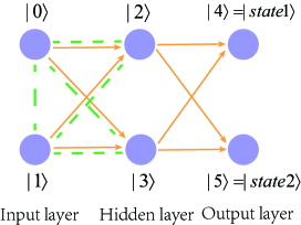
Figure 1: It is the graph representation of the quantum stochastic neural network (QSNN) used for quantum state binary discrimination. The state of the QSNN can be represented by a density matrix in the $N=6$ dimensional Hilbert space constituted by an orthogonal basis $\{|i\rangle\}_{i=0}^{5}$. The state of the two neurons of the input layer is initialized as the state of a 2-level input quantum state. Two neurons in the output layer correspond to the 2 labels $state1$ and $state2$ that distinguish two different states. The vertices are decoherently connected (orange lines with arrows) by Lindblad operators and coherently connected (green dashed lines) by Hamiltonian elements.

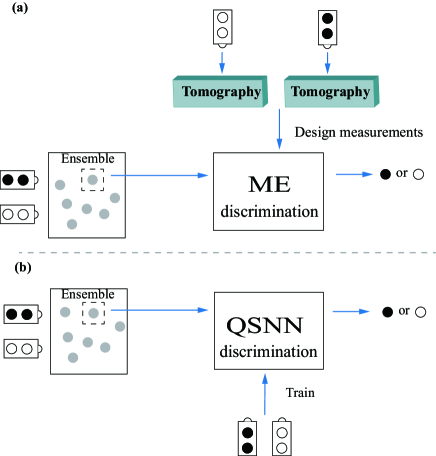
Figure 2: The flow charts of quantum state binary discrimination task. Black and white dots respectively represent the unknown quantum states from two different devices, and they become indistinguishable (gray dots) when mixed in an ensemble. The task is that we randomly pick one state from the ensemble and determine which device the state is coming from. (a) The minimum error discrimination. Before the discrimination, a pre-processing of quantum state tomography is often needed to get the complete information of the unknown states. (b) The QSNN discrimination. There is no need to obtain any prior information of quantum states through tomography in our approach. The network can discriminate quantum states after being trained with some labeled samples.

As shown in Fig. 2(a), before discriminating two unknown states in the ensemble with ME discrimination, a pre-processing of quantum state tomography is often needed, so that the appropriate measurement can be set up. It is not trivial to find the ME measurement set-up in general cases, but for the quantum state binary discrimination, the minimum error probability is given analytically by Helstrom helstrom1969quantum and Holevo holevo2011probabilistic , which is called the Helstrom bound:

$$P_{\text{H}}^{\text{error}}=\frac{1}{2}(1-\text{Tr}|w_{2}\rho_{2}-w_{1}\rho_{1}|).$$ (6)

Then, the success probability of the ME discrimination is given as

$$P_{\text{H}}=1-P_{H}^{error}.$$ (7)

However, as shown in Fig. 2(b), tomography is not required before our QSNN discrimination. The QSNN can discriminate quantum states by learning from some labeled samples, without knowing the mathematical expressions of these states. In order to complete the quantum state binary discrimination task, the QSNN is constructed by 6 neurons divided into three layers, as shown in Fig. 1. Some discussions about the topology of the network are given in SM I. There are only two sample states in the training set, namely $\rho_{1}$ and $\rho_{2}$. They are labeled $state\ 1$ and $state\ 2$, and fed into the QSNN with the prior probability $w_{1}$ and $w_{2}$, respectively. Thus, according to Eq. (4), the average success probability that the QSNN correctly gives the labels of the two input states is given as

$$P_{\text{N}}=\sum_{s=1}^{2}w_{s}\text{Tr}(\rho_{\text{out}}^{s}\varOmega^{s}).$$ (8)

Then, the loss function is defined as the distance between 1 and the average success probability, that is,

$$\mbox{Loss}=1-P_{\text{N}}.$$ (9)

In our simulation, we choose $w_{1}=w_{2}=0.5$. To show the performance of our approach, we compare the success probability of the QSNN ($P_{\text{N}}$) and that of the ME discrimination ($P_{\text{H}}$).

First, without loss of generality, we consider the quantum states

$$|\psi_{\theta}\rangle=\cos{\theta}|0\rangle+\sin{\theta}|1\rangle$$ (10)

in the real vector space. Here $\{|0\rangle,|1\rangle\}$ constitutes an orthogonal basis. The specific expressions of the quantum states selected here are intended only to mathematically evaluate the performance of our model. The states we want to discriminate against are $|\psi_{0}\rangle$ and $|\psi_{\theta}\rangle$, so our training set is $\{(|\psi_{0}\rangle,state1),(|\psi_{\theta}\rangle,state2)\}$. In our simulation, we train the QSNN with different training sets separately, where $\theta=0,\frac{\pi}{6},\frac{2\pi}{6},\frac{3\pi}{6},\cdots,\frac{11\pi}{6}$. The average success probability of the QSNN (blue curve) for the discrimination of 12 quantum state pairs ($|\psi_{0}\rangle$, $|\psi_{\theta}\rangle$) increases with the number of iterations used in the training procedure, as shown in Fig. 3(a). Our QSNN approximately achieves the optimal theoretical bound of the success probability named as Helstrom bound (red dashed line) after about 30 iterations. The optimal success probability of the QSNN for each training set with different $\theta$ is shown as a blue dot in Fig. 3(b). Each of them approximates to the Helstrom bound well.

Second, we consider the quantum states

$$|\psi_{\varphi}\rangle=\frac{\sqrt{2}}{2}(|0\rangle+e^{i\varphi}|1\rangle),$$ (11)

which are in a complex space. Similarly, we train the QSNN to discriminate states $|\psi_{0}\rangle$ and $|\psi_{\varphi}\rangle$ with the different training sets $\{(|\psi_{0}\rangle,state1),(|\psi_{\varphi}\rangle,state2)\}$, which are different in $\varphi=0,\frac{\pi}{6},\frac{2\pi}{6},\frac{3\pi}{6},\cdots,\frac{11\pi}{6}$. The result shown in Fig. 3(c) is also the average success probabilities for all training sets. We can see a certain gap between the success probability of the QSNN and the Helstrom bound. Fig. 3(d) indicates that the trained QSNN does not perform well in discriminating the quantum states with complex amplitudes. Even so, the discrimination result given by the optimized QSNN is still referential, because it can achieve a success probability of no less than 91% of the theoretical optimum.

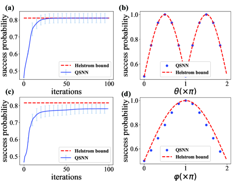
Figure 3: (a) The blue curve represents the average success probability of the QSNN for the discrimination of different quantum state pairs $(|\psi_{0}\rangle,|\psi_{\theta}\rangle)$ with real amplitudes. The red dashed line shows the average optimal theoretical value given by the minimum error discrimination. The results are given by taking the average over the success probabilities corresponding to all state pairs with different values of $\theta$. The error bars are plotted from the variances. The average success probability rises rapidly, and after about 30 iterations, it achieves the Helstrom bound. (b) The optimal success probabilities of the QSNN in discriminating $|\psi_{0}\rangle$ and $|\psi_{\theta}\rangle$ with each $\theta$ are drawn as blue dots. The Helstrom bound is shown as the red dashed line. Here, (c) and (d) include the results similar to (a) and (c), respectively. They are given by replacing the state represented by Eq. (10) with that represented by Eq. (11). The QSNN can achieve a success probability of no less than 91% of the theoretical optimum.

In summary, the QSNN can complete binary discrimination of unknown quantum states without tomography. It can be trained to its optimum after a few iterations and used to discriminate the states with a single detection. The optimized QSNN can achieve a success probability close to the Helstrom bound for both pure and mixed state (displayed in SM III) discrimination. Our model also works when the dimension of quantum states to be discriminated against is greater than 2, and we show the simulation result of the 3-qubit case in Fig. S8 of the SM. In addition, our approach is not limited by the number of states to be discriminated against theoretically, as shown in SM IV. In opposite, in general, if the number of the states is greater than two, the optimal measurement will be hard to be analytically developed in the fashion of traditional strategies.

Results – Classification of Entangled and Separable States. Entanglement is a primary feature of quantum mechanics, which is also considered with a resource. As the carrier of entanglement, entangled quantum states are costly to produce. Therefore, determining whether the given state is entangled or not is an important topic in quantum information theory. Now, some unknown separable states and entangled quantum states are mixed in an ensemble. We only know that they are prepared by two devices with an equal prior probability, without knowing their mathematical expressions. The task we consider in the following is to determine which category each quantum state belongs to. This is a classification task.

Several traditional strategies have been proposed to complete this task. For example, the positive partial transpose (PPT) criterion horodecki1995violating is both sufficient and necessary for 2-qubit entanglement detection with the requirement of quantum tomography (see Fig. S9 of the SM). The CHSH inequality bell1964einstein ; clauser1969proposed is also an attractive strategy because it only needs partial information of the quantum states (see Fig. S9 of SM). However, on the one hand, multiple measurements are still required. On the other hand, using fixed measurements, the CHSH inequality can’t detect all entangled states in a set of states. To optimize the accuracy of the entanglement detection using the CHSH inequality, classical artificial neural networks combined with machine learning techniques have been proposed in Refs. gao2018experimental ; ma2018transforming . They construct a quantum state classifier and it achieves the accuracy of the classification to near unity, but multiple measurements are still required. To avoid multiple measurements or state tomography, we train a QSNN to be a quantum classifier.

In order to evaluate our approach more clearly, we select an unknown set of Werner-like states in our simulation. Each state is of the form

$$\rho=p|\varPsi\rangle\langle\Psi|+(1-p)\frac{I}{4},$$ (12)

where $|\varPsi\rangle=(U_{1}\otimes U_{2})|\psi_{+}\rangle$ and the real coefficient $p\in[0,1]$. $U_{1}$ and $U_{2}$ are two unknown local unitaries acting on the Bell states $|\psi_{+}\rangle=\frac{\sqrt{2}}{2}(|01\rangle+|10\rangle)$. The state $\rho$ can be regarded as the convex combination of an unknown maximally-entangled state and the maximally mixed state $\frac{I}{4}$. The quantum state $\rho$ is separable when $p\leq\frac{1}{3}$ and it is entangled otherwise.

In our simulation, there are four neurons in the input layer and four in the hidden layer. Two neurons in the output layer correspond to two labels $l^{s}$: reparable $S$ and entangled $E$. To be more specific, if the final state $\rho_{\text{out}}$ is $|S\rangle\langle S|$ ($|E\rangle\langle E|$), the trained QSNN shows that the input quantum state is separable (entangled). Performing a corresponding measurement $\varOmega^{s}=|l^{s}\rangle\langle l^{s}|$ on the final state $\rho_{\text{out}}^{s}$ gives the probability that the QSNN gives the label of the $s$th input state correctly. The loss function is defined as the mean error probability of all the $M$ training samples

$$\mbox{Loss}=1-\frac{1}{M}\sum_{s=1}^{M}\text{Tr}(\rho_{\text{out}}^{s}\varOmega^{s}).$$ (13)

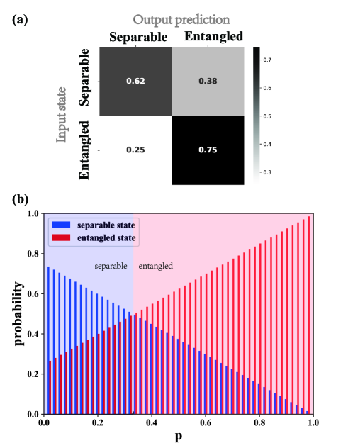
Figure 4: (a) The classification confusion matrix of the QSNN. The numbers in it are the mean success and error probabilities of the QSNN in classifying the 49 samples represented by Eq. (12) with $p\in\{0.02\cdot n\}_{n=1}^{49}$. The QSNN performs better when the input states are entangled. (b) The classification result of each state with a specific value of $p$. The bar chart shows the probabilities that the trained network identifies the 49 input states as entangled states (red bars) and separable states (blue bars). The whole chart is divided by $p=\frac{1}{3}$ into the light blue area (the state is separate) and the light red area (the state is entangled). The success probabilities are always higher than the error probabilities.

For the example of $U_{1}=\sigma_{z}$, $U_{2}=I$, we numerically give the classification results. We only use $M=4$ training samples, where $p\in\{0,0.2,0.4,0.8\}$, while use 49 states with $p\in\{0.02\cdot n\}_{n=1}^{49}$ to evaluate the performance of the trained QSNN in the simulation. The classification confusion matrix for these 49 states is shown in Fig. 4(a). The trained QSNN identifies separable states successfully with the probability of 0.62 and identifies entangled states successfully with the probability of 0.75. The probability of one kind of the wrong classifications, i.e., the trained network identifies a separable state as an entangled one, is 0.38. The probability of the other kind of wrong classifications is 0.25.

The probabilities that each quantum state with a specific value of $p\in\{0.02\cdot n\}_{n=1}^{49}$ is identified as a separable state (blue bar) and an entangled state (red bar) are shown in Fig. 4(b). When the input states are entangled at $1/3<p\leq 1$ (light red region), the red bars are always longer than blue bars. It means that the success probabilities are always higher than the error probabilities, which is also true when $0\leq p\leq 1/3$ (light blue region).

In summary, when given an unknown quantum state set, the QSNN can be trained by several labeled states and used to classify the others. Although the QSNN becomes confused about the states at the boundary $p=1/3$, the success probability is always higher than the error probability for each state. What’s more, the trained QSNN can give the classification result only using a single detection for each state. Some details about the parameters and hyperparameters of the QSNN are given in SM V.

In this work, we have introduced the quantum stochastic neural network (QSNN), based on quantum stochastic walks. When combined with machine learning, it can be trained to become a quantum state classifier.

If one wants to classify an ensemble only containing two unknown quantum states, the classification task becomes binary discrimination. The QSNN doesn’t need any information of the candidate states in advance, so it avoids the experimentally expensive quantum state tomography used in the traditional minimum error discrimination. We have benchmarked the QSNN’s performance in the quantum state binary discrimination tasks with numerical simulation. The success probability of the QSNN turned out to be very close to the theoretical optimal success probability, i.e., the Helstrom bound.

When given an unknown ensemble containing states from two different families, the QSNN can be trained to classify them into those two families. We show an example of classifying Werner-like states according to whether they are entangled or not. For all those states, the trained QSNN is always more likely to classify it into the correct family with a single detection. The optimal performance of the QSNN can be achieved with only four training samples, while avoiding the state tomography and multiple measurements required by other classification methods such as using the PPT criteria or the CHSH inequality. This also suggests that our approach may reduce the consumption of resources compared to traditional methods.

All the present results have shown the potential of the QSNN as a general-purpose quantum classifier, which may be helpful in various quantum machine learning models, such as the quantum adversarial generative networks dallaire2018quantum .

Acknowledgments. This work is supported by the National Key R&D Program of China (Grant No. 2017YFA0303703) and the National Natural Science Foundation of China (Grant No. 12175104).

References

- (1) Helstrom C W 1969 Journal of Statistical Physics 1 231
- (2) Ivanovic I D 1987 Phys. Lett. A 123 257
- (3) Dieks D 1988 Phys. Lett. A 126 303
- (4) Peres A 1988 Phys. Lett. A 128 19
- (5) Horodecki R, Horodecki P and Horodecki M 1995 Phys. Lett. A 200 340
- (6) Horodecki M, Horodecki P and Horodecki R 1996 Phys. Lett. A 223
- (7) Terhal B M 2000 Phys. Lett. A 271 319
- (8) Lewenstein M, Kraus B, Cirac J I and Horodecki P 2000 Phys. Rev. A 62 052310
- (9) Bell J S 1964 Physics Physique Fizika 1 195
- (10) Clauser J F, Horne M A, Shimony A and Holt R A 1969 Phys. Rev. Lett. 23 880
- (11) Massar S and Popescu S 2005 Asymptotic Theory Of Quantum Statistical Inference: Selected Papers 356
- (12) Bruß D and Macchiavello C 1999 Phys. Lett. A 253 249
- (13) Paris M and Rehacek J 2004 Quantum State Estimation (New York: Springer Science & Business Media)
- (14) Bergou J A 2010 Journal of Modern Optics 57 160
- (15) Barnett S M and Croke S 2009 Advances in Optics and Photonics 1 238
- (16) Das Sarma S, Deng D L and Duan L M 2019 Physics Today 72 48
- (17) Carleo G, Cirac I, Cranmer K, Daudet L, Schuld M, Tishby N, Vogt-Maranto L and Zdeborová L 2019 Rev. of Mod. Phys. 91 045002
- (18) Schuld M, Bocharov A, Svore K M and Wiebe N 2020 Phys. Rev. A. 101 032308
- (19) Li W and Deng D L 2022 Science China Physics, Mechanics & Astronomy 65 1
- (20) Biamonte J, Wittek P, Pancotti N, Rebentrost P, Wiebe N and Lloyd S 2017 Nature 549 195
- (21) Dunjko V and Briegel H J 2018 Reports on Progress in Physics 81 074001
- (22) He Z, Li L, Zheng S, Li Y and Situ H 2021 New Journal of Physics 23 033002
- (23) Beer K, Bondarenko D, Farrelly T, Osborne T J, Salzmann R, Scheiermann D and Wolf R 2020 Nature communications 11 1
- (24) Steinbrecher G R, Olson J P, Englund D and Carolan J 2019 npj Quantum Inf. 5 1
- (25) Carleo G and Troyer M 2017 Science 355 602
- (26) Gao X and Duan L M 2017 Nature communications 8 1
- (27) Wan K H, Dahlsten O, Kristjánsson H, Gardner R and Kim M 2017 npj Quantum Inf. 3 1
- (28) Bondarenko D and Feldmann P 2020 Phys. Rev. Lett. 124 130502
- (29) Chen H, Wossnig L, Severini S, Neven H and Mohseni M 2021 Quantum Machine Intelligence 3 1
- (30) Patterson A, Chen H, Wossnig L, Severini S, Browne D and Rungger I 2021 Phys. Rev. Res. 3 013063
- (31) Cong I, Choi S and Lukin M D 2019 Nature Physics 15 1273
- (32) Dalla Pozza N and Caruso F 2020 Phys. Rev. Res. 2 043011
- (33) Laneve A, Geraldi A, Hamiti F, Mataloni P and Caruso F 2021 arXiv:2107.09968 [quant-ph]
- (34) Whitfield J D, Rodríguez-Rosario C A and Aspuru-Guzik A 2010 Phys. Rev. A 81 022323
- (35) Schuld M, Sinayskiy I and Petruccione F 2014 Phys. Rev. A 89 032333
- (36) Tang H, Feng Z, Wang Y H, Lai P C, Wang C Y, Ye Z Y, Wang C K, Shi Z Y, Wang T Y, Chen Y, Gao J and Jin X M 2019 Phys. Rev. Appl. 11 024020
- (37) Farhi E and Gutmann S 1998 Phys. Rev. A 58, 915
- (38) Kossakowski A 1972 Reports on Mathematical Physics 3 247
- (39) Lindblad G 1976 Communications in Mathematical Physics 48 119
- (40) Gorini V, Kossakowski A and Sudarshan E C G 1976 J. Math. Phys. 17 821
- (41) Holevo A S 2011 Probabilistic and statistical aspects of quantum theory (Springer Science & Business Media)
- (42) Gao J, Qiao L F, Jiao Z Q, Ma Y C, Hu C Q, Ren R J, Yang A L, Tang H, Yung M H and Jin X M 2018 Phys. Rev. Lett. 120 240501
- (43) Ma Y C and Yung M H 2018 npj Quantum Inf. 4 1
- (44) Dallaire-Demers P L and Killoran N 2018 Phys. Rev. A 98 012324