CLIP Surgery for Better Explainability with Enhancement in Open-Vocabulary Tasks

Abstract

Contrastive Language-Image Pre-training (CLIP) is a powerful multimodal large vision model that has demonstrated significant benefits for downstream tasks, including many zero-shot learning and text-guided vision tasks. However, we notice some severe problems regarding the model’s explainability, which undermines its credibility and impedes related tasks. Specifically, we find CLIP prefers the background regions than the foregrounds according to the predicted similarity map, which contradicts human understanding. Besides, there are obvious noisy activations on the visualization results at irrelevant positions. To address these two issues, we conduct in-depth analyses and reveal the reasons with new findings and evidences. Based on these insights, we propose the CLIP Surgery, a method that enables surgery-like modifications for the inference architecture and features, for better explainability and enhancement in multiple open-vocabulary tasks. The proposed method has significantly improved the explainability of CLIP for both convolutional networks and vision transformers, surpassing existing methods by large margins. Besides, our approach also demonstrates remarkable improvements in open-vocabulary segmentation and multi-label recognition tasks. For examples, the mAP improvement on NUS-Wide multi-label recognition is 4.41% without any additional training, and our CLIP Surgery surpasses the state-of-the-art method by 8.74% at mIoU on Cityscapes open-vocabulary semantic segmentation. Furthermore, our method benefits other tasks including multimodal visualization and interactive segmentation like Segment Anything Model (SAM). The code is available at https://github.com/xmed-lab/CLIP_Surgery

1 Introduction

Providing explanations for neural network predictions can enhance their transparency and credibility, which has become a crucial consideration across various fields of application, such as medical diagnosis van2022explainable , auto driving zablocki2022explainability , semantic segmentation wang2020self ; li2021pseudo ; zabari2021semantic , object localization selvaraju2017grad ; wei2021shallow ; gao2021ts and image generation bar2022text2live ; vinker2022clipasso . With the advancements of convolutional neural networks (CNNs), various methods have emerged to explain neural networks, such as class activation map zhou2016learning ; selvaraju2017grad ; chattopadhay2018grad ; wang2020score , feature visualization olah2017feature ; nguyen2019understanding and model sensitivity ribeiro2016should . Recently, Contrastive Language-Image Pre-training (CLIP), a powerful large multimodal pre-training model, has been proposed, which can benefit many downstream tasks such as recognition conde2021clip ; sun2022dualcoop ; tian2022vl , segmentation zhou2022extract ; liu2022open ; shin2022reco , detection gu2021open ; esmaeilpour2021zero and generation ramesh2022hierarchical ; rombach2022high ; singer2022make ; bar2022text2live ; ruiz2022dreambooth . However, unlike CNNs, the model explainability of CLIP has been less explored.

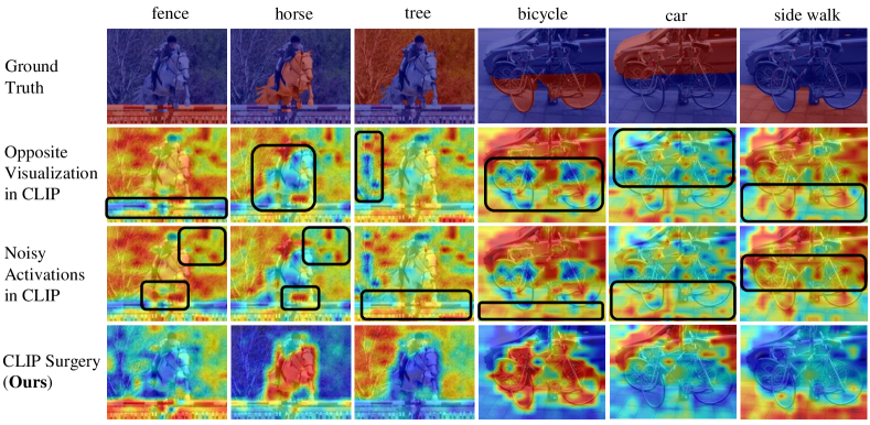
Figure 1: Two major observations of CLIP: opposite visualization and noisy activations. The class activation maps are visualized by the similarity map defined in Eq. 1 (fundamental raw predictions of CLIP), where the foreground regions are marked in red and the background regions are colored in blue. We observe that the original CLIP deems foregrounds as backgrounds (see black boxes in the second row), exhibiting opposite visualization results against the ground truth. Besides, there are many noisy activations on background regions; see black boxes in the third row. Our CLIP surgery, consisting of architecture surgery and feature surgery, can correct these problems, providing reasonable visualizations in good quality.

Most existing explainability methods are designed for single modality models that are trained in a fully supervised manner. However, conventional explainability methods yield poor visualization results when directly applied to CLIP, a multimodal model trained with both image and text. For example, Fig. 9 shows that both gradient-based methods selvaraju2017grad for CNN and attention-based methods lapuschkin2019unmasking for vision transformers (ViT) dosovitskiy2020image render degraded results when applied to CLIP. In addition to the single modality explainability methods, multimodal explainability methods also perform poorly on CLIP; see results of Bi-Modal chefer2021generic built upon explainability of ViT chefer2021transformer and gScoreCAM chen2022gscorecam for CLIP-based localization in Fig. 9. Another approach goh2021multimodal visualizes CLIP’s activated neurons by images generation with particular neuron families such as people neurons, emotion neurons and region neurons. However, this method can not localize the discriminative regions as the class attention map (CAM) zhou2016learning used in above methods, limiting its further application in downstream tasks.

To address the above limitations, we propose a novel CLIP Surgery method which brings better explainability with direct enhancements in multiple open-vocabulary tasks, all without requiring additional training efforts. CLIP Surgery consists of CLIP Architecture Surgery and CLIP Feature Surgery, which are motivated by two major observations shown in Fig. 1: opposite visualization and noisy activations. Specifically, opposite visualization refers to the visualization results that are opposite to the ground-truth. We discovered that the major cause of this issue is the parameters (query and key) in the self-attention module, which heavily focus on opposite semantic regions; see visualization in Fig. 4. To address this issue, we replace the original self-attention via the proposed v-v self-attention. In addition, we observed that the features generated by feed-forward networks (FFNs) are considerably different from the final feature; see Fig. 5. Therefore, we propose a new approach, called dual paths, to skip these layers during inference. The above modifications to the architecture for inference are referred to as CLIP Architecture Surgery.

Our second observation: noisy activations refers to the obvious highlights on background regions, which often appear on irrelevant regions in spot shape; see Fig. 1 and Fig. 6. We attribute the cause to the common yet redundant features present in CLIP. To support our argument, we examine the similarity maps for different labels and observe that noisy activations occur across multiple labels, as depicted in Fig. 7. We use an empty string to eliminate irrelevant and redundant features. It has been discovered that activations from these redundant features have a correlation with the positive labels. Based on the above observations, we propose the CLIP Feature Surgery to identify and remove these redundant features. Our solution effectively mitigates these noisy activations, as shown in the last row of Fig. 1, and visualizes CLIP in good quality; see Fig. 8.

Further experiments demonstrate the outstanding effectiveness and wide applicability of the proposed CLIP Surgery. Compared with CLIP in terms of explainability, the maximal improvements are 38.42% at mIoU and 72.48% at metric mSC (score difference between foregrounds and backgrounds) in Tab. 3. When applying to open-vocabulary tasks, our method boosts the multi-label recognition task by 4.41% at mAP metric on NUS-Wide chua2009nus . And our method outperforms the state-of-the-art open segmentation method at mIoU by 4.56%, 4.44%, and 8.74% on PASCAL Context mottaghi2014role , COCO Stuff caesar2018coco , and Cityscapes cordts2016cityscapes , respectively. In addition, our method demonstrates wide applicability and has benefited tasks such as interactive segmentation like Segment Anything Model (SAM) kirillov2023segment and multimodal visualization.

In summary, this paper has the four main contributions:

• We observe that CLIP exhibits opposite visualization and noisy activations. Then, we identify that parameters (query and key) in self-attention layer cause the opposite visualization, and the redundant features are the reason for noisy activations.

• Based on these findings, we propose the CLIP Surgery, consisting of architecture and feature surgery, which solve the observed explainability problems effectively.

• We demonstrated that our CLIP surgery produces much better explainability performance across various backbones and datasets. Besides, we conduct multimodal visualization to explain the image-text pairs in CLIP’s training process, beyond conventional single modality explainability methods.

• Our CLIP surgery also enhances downstream open-vocabulary semantic segmentation, interactive segmentation, and multi-label recognition tasks by large margins (e.g., 4.41% at mAP for the recognition, 8.74% at mIoU for the semantic segmentation, and 12.95% at points accuracy for in interactive segmentation).

2 Related Works

This paper aims to improve the visual explainability of CLIP and enhance downstream tasks such as open-vocabulary semantic segmentation and open-vocabulary multi-label recognition. Below, we conduct a literature review on related work.

2.1 Explainability of CLIP

Recently, Contrastive Language-Image Pre-training (CLIP) radford2021learning has emerged as a large vision model supervised by natural language. Before the emergence of CLIP, traditional explainability methods zeiler2014visualizing ; zhou2016learning are designed for convolutional neural networks (CNNs). And the followed works selvaraju2017grad ; chattopadhay2018grad ; wang2020score continuously boost the quality of class attention map (CAM) zhou2016learning . Recent methods chefer2021transformer have focused on explainability for vision transformers dosovitskiy2020image based on self-attention and gradient. However, these methods are typically designed for fully-supervised single modality models and have shown poor results on CLIP, which is a multimodal model supervised by natural language and images. Later on, Bi-Modal chefer2021generic was proposed for explainability on multimodal model, and gScoreCAM chen2022gscorecam was introduced for the explainability of CLIP to object localization task. However, despite their efforts, the results of these methods remain unsatisfactory; see results in Table 4. In particular, they tend to perform poorly for dense predictions with larger output size, as demonstrated in Table 5. Another method specifically designed for CLIP is RCLIP li2022exploring , which aims to address the problem of opposite visualizations by reversing CLIP’s results that achieves better visualization results than existing explainability methods. Additionally, a trainable version of RCLIP called ECLIP li2022exploring was proposed, which further improves performance. However, ECLIP requires fine-tuning to adapt to new layers, making it a more complex method compared to others.

Our CLIP surgery surpasses existing methods in three aspects: (1) Effectiveness. Compared to other methods, our CLIP surgery shows significantly improved performance, as shown in Table 4 and Fig. 9, respectively. (2) Practicalness and Efficiency. Our method is more practical than other methods selvaraju2017grad ; lapuschkin2019unmasking ; chefer2021transformer ; chen2022gscorecam ; li2022exploring as it only requires inference once and does not need any fine-tuning or backpropagation for labels multiple times, making it easier to implement in practice. (3) Flexibility. Our method is not limited in terms of the output size, making it suitable for dense prediction tasks such as segmentation. Additionally, it improves the performance of multi-label recognition without the need of fine-tuning, without annotation for seen classes of previous works xu2022dual ; sun2022dualcoop . These advantages collectively demonstrate the importance and novelty of our approach for enhancing the explainability of CLIP.

2.2 Open-Vocabulary Semantic Segmentation

Open-vocabulary semantic segmentation zhou2022extract ; liu2022open ; shin2022reco ; xu2022groupvit refers to segment semantic regions via textual names or descriptions for the open world without any mask annotations. Compared to conventional zero-shot semantic segmentation bucher2019zero ; xu2021simple , which consist of seen classes with pixel-level supervision and unseen classes, open-vocabulary setting only requires image-text pairs during training phase, without any pixel-level annotations. According to the complexity, we broadly divide the existing methods into three groups: (1) The first group requires additional model or information, such as fully supervised proposal network in RegionCLIP zhong2022regionclip , multifarious supervisions in GLIPv2 zhang2022glipv2 , extra unsupervised model in zabari2021semantic and fully supervised saliency model in NamedMask shin2022namedmask , which are complex in supervision. Since these methods use extra information or models beyond image-text pairs, we did not include them in our experiments to ensure a fair comparison. (2) The second group conducts additional training processes, while additional model or information in the first group are not used. For instances, retrieval process of Reco shin2022reco , clustering steps in ViL-Seg liu2022open , training from scratch to adapt the added grouping layers in GroupViT xu2022groupvit and SegCLIP luo2022segclip . These methods require fine-tuning on target datasets, or training from scratch using massive data for pre-training, which is complex in training process. (3) The third type requires neither extra supervision nor additional training process. One of the representative methods is MaskCLIP zhou2022extract , which modifies the original CLIP without any fine-tuning.

Our method belongs to the third group with the least complexity. However, our approach differs from MaskCLIP zhou2022extract in the following ways: (1) Our objective is to improve explainability, while MaskCLIP aims to extract dense predictions for segmentation. (2) Instead of deleting the self-attention in MaskCLIP, we propose the v-v self-attention to reform the original attention module. (3) Additionally, we introduce dual paths to merge multiple v-v self-attentions rather than modifying only the last layer as in MaskCLIP.

2.3 Open-Vocabulary Multi-Label Recognition

Open-vocabulary multi-label recognition refers to classify multi-label images via textual names or descriptions for the open world without any seen categories. The key differences between open-vocabulary setting and fully supervised setting is that fully supervised methods use binary cross-entropy loss with sigmoid as post-processing, while open-vocabulary method radford2021learning applies contrastive loss with softmax operation. Another setting: zero-shot multi-label recognition norouzi2013zero ; akata2015label ; narayan2021discriminative ; ben2021semantic differs from open-vocabulary multi-label recognition at the supervision. Specifically, open-vocabulary method are supervised by natural language, while zero-shot methods are supervised by manual label on seen categories and conduct open test on unseen categories. For these zero-shot methods based on CLIP, Dual Modality xu2022dual aligns visual and textual features via a DM-encoder. DualCoOp sun2022dualcoop , and TaI-DPT guo2022texts achieve quickly adaption to pre-trained vision-language model. MTK he2022open exploits multi-modal knowledge of image-text pairs. Our method is complementary to the above zero-shot algorithms, and it’s easy to apply with new state-of-the-art performances. Since we just need to conduct CLIP Feature Surgery on their outputs without any fine-tuning. Besides, our method greatly boosts the performance of CLIP in open-vocabulary setting, without any supervision from seen categories of zero-shot setting, with lower complexity and annotation cost.

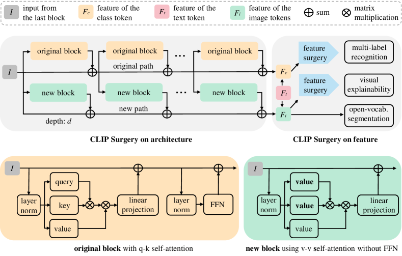
Figure 2: Framework of CLIP Surgery. For the architecture, we propose the dual paths. Specifically, the original path uses the original block with q-k self-attention in Eq. 2, and the new block applies the proposed v-v self-attention in Eq. 3 without feed-forward network (FFN), starting from depth $d$. Note, the parameters of the new block are copied from the original block. Then we deploy the feature surgery in Eq. 9 to features of image tokens $\boldsymbol{F}_{i}$ with text features $\boldsymbol{F}_{t}$ for explainability task. And the feature of class token $\boldsymbol{F}_{c}$ from the original path is processed by feature surgery for multi-label recognition.

3 CLIP Architecture Surgery to Correct Opposite Visualization

In this section, we aim to address the problem of opposite visualization, and present the first part of our proposed CLIP Surgery; see Fig. 2. To be specific, the left top part is the CLIP Architecture Surgery, with its detailed blocks at the bottom. This section is structured into four parts: problem, reason, analyze, and solution, in order to provide a clear and organized discussion.

3.1 Problem of Opposite Visualization

Foremost, we visually explain the CLIP from the similarity map, which refers to the class attention map from the raw predictions of CLIP. Here, the raw predictions are the similarity distances between the text feature and image features of multiple image tokens. This similarity map is the most fundamental and direct explainability cue of CLIP, since it does not require any extra operation like back-propagation. To be specific, we compute the similarity distance between features of image tokens $\boldsymbol{F}_{i}\in\mathbb{R}^{N_{i}\times C}$ ($N_{i}$ is the number of image patches) and transposed features of texts $\boldsymbol{F}_{t}\in\mathbb{R}^{N_{t}\times C}$ with L2 normalization $\|\ \|_{2}$ along $C$ dimension as Eq. 1.

$$\boldsymbol{M}=norm(resize(reshape(\frac{\boldsymbol{F}_{i}}{\|\boldsymbol{F}_{i}\|_{2}}\cdot(\frac{\boldsymbol{F}_{t}}{\|\boldsymbol{F}_{t}\|_{2}})^{\top}))),$$ (1)

Here, $\boldsymbol{M}\in\mathbb{R}^{H\times W\times N_{t}}$ is the similarity map (also image-text similarity map in li2022exploring ), where $H,W$ indicate the height and width of original image. We reshape and resize image tokens in number $N_{i}$ to $H\cdot W$ via bilinear interpolation, with min-max normalization $norm()$.

Subsequently, we generate similarity maps of CLIP, as shown in Figure 3, and observe that the most prominent problem is the opposite visualization. More specifically, when identifying a target category, CLIP tends to prioritize background regions over foreground regions, which contradicts human perception. This phenomenon is observed across various backbones (ResNets he2016deep and Vision Transformers dosovitskiy2020image ), also occurs in multiple explainability methods as shown in Fig. 9. This figure indicates it is a common problem instead of an isolated case. Besides, some works may generate reasonable visualization from CLIP, but extra supervision Rao_2022_CVPR or additional models xu2021simple ; zhong2022regionclip ; zhang2022glipv2 are needed beyond conventional explainability methods.

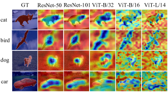
Figure 3: CLIP shows opposite visualization against the ground truth “GT” for both ResNets he2016deep and ViTs dosovitskiy2020image .

3.2 Reason and Evidence

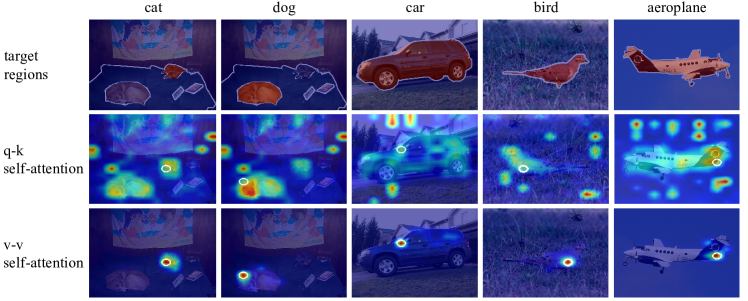
Figure 4: Visual comparison between q-k self-attention (Eq. 2) of CLIP and our v-v self-attention (Eq. 3). These attention maps are from the last self-attention layer at the token, whose score is the highest over other image tokens (marked with white circle). The original q-k self-attention in the second row pays much attention on the opposite semantic regions, while our v-v self-attention links nearby tokens at the same semantics.

Firstly, let us draw the conclusion regarding the reason: the parameters key and query in self-attention link features from opposite semantic regions. To substantiate our claim, we present evidence in Fig. 4. In this figure, q-k self-attention $Attn_{qk}$ indicates the original self-attention of CLIP as:

$$Attn_{qk}=softmax(\boldsymbol{Q}\cdot\boldsymbol{K}^{\top}\cdot scale)\cdot\boldsymbol{V}\ ,$$ (2)

where $\boldsymbol{Q},\ \boldsymbol{K},\ \boldsymbol{V}$ are the features after applying parameters $\phi_{q},\ \phi_{k},\ \phi_{v}$ with learned logit scale. And v-v self-attention $Attn_{vv}$ computes self-attention for feature from parameter value itself, without $\phi_{q},\phi_{k}$ as:

$$Attn_{vv}=softmax(\boldsymbol{V}\cdot\boldsymbol{V}^{\top}\cdot scale)\cdot\boldsymbol{V}\ .$$ (3)

Based on our analysis, we find those erroneous parameters (query and key) in the self-attention is the underlying reason of opposite visualization. From Fig. 4, we can see that the original q-k attention focus a lot on opposite semantic regions. It means the relation map is confused, where foreground information are embedded into features of foreground tokens, while the proposed v-v attention is good. It makes sure the cosine distance on itself is the highest, and nearby tokens are highlighted, instead of paying attention to irrelevant regions. This evidence indicates problematic parameters in self-attention lead to confused relation, which allows tokens are identified into opposite meaning.

This problem is also discussed in ECLIP li2022exploring , their reason is the shifted feature in the pool layer. Different from it, we explore the underlying reason in the inference phase, instead of pooling layer in training. Here, we can correct erroneous self-attention for multiple layers in vision transformers dosovitskiy2020image during inference, instead of the last pooling layer during training in ECLIP. Therefore, analyzing the self-attention helps us to correct explainability for multiple layers without training, and make it more readily applicable to downstream tasks without fine-tuning.

3.3 Analyze for Multiple Modules

Besides the confused relation map in self-attention, we investigate the explainability of CLIP for multiple modules via cosine of angle. Specifically, we compute the cosine of angles $a<\ >$ between text feature $\boldsymbol{F}_{i}$ and feature of a certain module at the class token $\hat{\boldsymbol{F}_{c}}$ as Eq. 4. Note that these modules include self-attention modules and feed-forward networks (FFN).

$$a<\boldsymbol{F}_{t},\hat{\boldsymbol{F}_{c}}>=\frac{\boldsymbol{F}_{t}\cdot\hat{\boldsymbol{F}_{c}}}{\|\boldsymbol{F}_{t}\|_{2}\cdot\|\hat{\boldsymbol{F}_{c}}\|_{2}}.$$ (4)

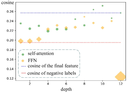
Figure 5: Cosine of angles (Eq. 4) for self-attentions and feed-forward networks (FFNs) at different depths. Features (scatters) close to the final feature (blue line) are marked at smaller size, with minimum adverse impact to the model. We can see that features of self-attentions are more closed to the final feature than FFNs. While some FFNs are near to the cosine of negative labels (red line). Note, results are the average value on VOC 2012 dataset everingham2010pascal .

Then we draw the cosine of angles for each module in Fig. 5. From this figure, we find FFN modules have larger gaps than self-attention modules, when computing the cosine of angle with the final classification feature. Especially, the last FFN returns the feature at cosine 0.1231, which is much farther than the cosine of negative labels. And features of first three FFNs are very close to the features of negative labels. This finding suggests that FFNs pushes features towards negatives when identifying positives, thus hurts the model. And Tab. 2 experimentally prove this claim in explainability task. Therefore, we only take features from the reformed self-attention modules without those of FFNs.

3.4 CLIP Architecture Surgery

In Section 3.2, it is observed that v-v self-attention establishes a connection within the same semantic region, unlike the original q-k self-attention, which produces a muddled attention map. Subsequently, we find that the features obtained from shallow self-attentions and FFNs are not proximal to the final image feature, as discussed in Sec. 3.3. Thus, avoiding the use of these features improves explainability and multi-label recognition. Building on these observations, we introduce the CLIP Surgery for the inference architecture, illustrated in Fig. 2.

Foremost, we propose a technique called dual paths to merge features from multiple v-v self-attention layers. The purpose of dual paths is to maintain stable input and keep the original features for classification task. Since we modify the structure of self-attention and drop many middle layers, CLIP will collapse if we only use one path to merge residues, as shown in Tab. 2. Because after first modification, the inputs of following modules are changed, and this difference will be amplified layer by layer, leading to model crash.

Here, we define the CLIP Surgery for the architecture by illustrating the update of dual paths as Eq. 5.

$$\hat{x}_{i+1} =\begin{cases}None&i<d\\ f_{attn_{vv}}(x_{i},\{\phi_{v}\})+x_{i}&i=d\\ f_{attn_{vv}}(x_{i},\{\phi_{v}\})+\hat{x}_{i}&i>d\end{cases},\ \forall T\&A$$ (5)

$$x_{i+1} =\begin{cases}\begin{split}f&{}_{FFN}(x_{i}^{\prime})+x_{i}^{\prime},\ s.t.\\ &x_{i}^{\prime}=f_{attn_{qk}}(x_{i},\{\phi_{q},\phi_{k},\phi_{v}\})+x_{i}\end{split}&,\ \forall T\&A\\ f_{res}(x_{i})+x_{i}&,\ \forall Res\end{cases}$$

Specifically, $\hat{x}_{i+1}$ is the output of new path where residues after surgery are gathered, and $x_{i+1}$ is the output of original path. For the new path, $i$ is the index of the block, and depth $d$ controls the start of the new path. For shallow layers under $d$, there is only the original path, and the new path returns “None”. For the first reformed self-attention ($i=d$), we merge $x_{i}$ from the original path with the output of $f_{attn_{vv}}(x_{i},\{\phi_{v}\})$, which is consisted of the v-v self-attention in Eq. 3 using parameter $\phi_{v}$ and a linear projection layer without Feed-Forward Networks $f_{FFN}$). For following modules $i>d$, the $x_{i}$ is turned to $\hat{x}_{i}$, where outputs of deeper self-attentions are merged only. This path is only applicable to Transformers and Attention pooling ($T\&A$) of CLIP. For the original path, transformers and the attention pooling deploy the original q-k self-attention in Eq. 2 with parameters $\phi_{q},\phi_{k},\phi_{v}$. And the original Feed-Forward Networks (fully connected layers) $f_{FFN}$ are required after $f_{attn_{qk}}$. For ResNets he2016deep their residue blocks $f_{res}$ like BottleNeck blocks are used as before. Note that the original path is not modified, while CLIP Surgery at the new path needs its previous output $x_{i}$ as stable inputs.

Unlike dual path networks chen2017dual which exchange information across paths and use the same structure for train and test phase, we only apply dual paths in inference phase and the new path is not used by the original path. Also, it’s different from existing explainability methods lapuschkin2019unmasking ; chefer2021generic for multiple layers. Our dual path allows merging features from multiple layers without back-propagation, which is faster and directer. Base on it, we modify the original self-attention modules to the proposed v-v self-attentions, and merge their outputs requiring inference only once. This is the first part of our CLIP Surgery, which corrects the problem of opposite visualization.

4 CLIP Feature Surgery to Mitigate Noisy Activations

This is the second section of our methodology. Here, we discuss the other explainability problem: noisy activations, then provide our reason, evidences, and solution. For easier understanding, we depict the CLIP Surgery on feature in this section at the right top part of Fig. 2. This figure indicates CLIP Surgery on feature is based on architecture surgery, then serves for explainability task and multi-label recognition task from the new path and original path, respectively.

4.1 Problem of Noisy Activations

The predicted similarity map in CLIP presents a significant challenge for explainability due to the presence of noisy activations. These activations appear as highlights in spot shapes at unexpected positions, representing a form of noise that undermines the credibility of CLIP. As illustrated in Figure 6, this issue is conspicuous and raises concerns about the reliance of CLIP’s decision-making on noisy regions instead of more discriminative areas. Furthermore, the noisy activations significantly degrade the quality of visualizations, resulting in spotty heatmaps with irregular shapes. It is therefore imperative that this issue is addressed in a careful and thorough manner.

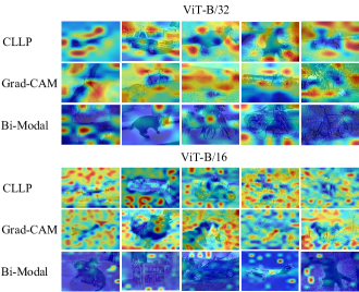
Figure 6: Noisy activation is universal for varied backbones and methods, including Grad-CAM selvaraju2017grad for convolutional neuron networks and Bi-Modal chefer2021generic for multi-modal vision transformers. These red activations on backgrounds are the noises at spot shape.

The problem of noisy activation is pervasive across various research papers, including explainability methods for convolutional neural networks (CNNs) selvaraju2017grad ; wang2020score , vision transformers chefer2021transformer , and CLIP li2022exploring ; chen2022gscorecam . However, researchers have paid little attention to this problem and have not provided adequate explanations for its occurrence. In other words, this problem is ubiquitous but under-explored.

4.2 Reason and Evidences

There are two simple hypotheses to explain noisy activations: false predictions and related context. In the case of false predictions, the model focuses on false regions when it predicts incorrectly. In the presence of related context, certain semantic features such as a lake and a boat may be highlighted together. However, as can be observed from Fig. 7, the noise across categories is uniform and similar, while false predictions and related context vary across categories in general. This indicates that these hypotheses cannot explain the underlying cause of noisy activations and suggests the need for further investigation.

Here, we propose that noisy activations are caused by redundant features in CLIP. To explain this, it is important to note that CLIP learns to recognize countless categories through natural language, which implies that only a few features are activated for a particular class, while other features remain non-activated for the rest of numerous classes. As a result, these non-activated features become redundant and occupy a significant portion of the feature space. The noisy activations observed in the similarity maps are a direct result of these redundant features being activated.

The first evidence is that the noise activations occur in the empty text label, as shown in Fig. 7. In this figure, we draw the similarity maps with positive textual labels and empty textual label. For empty label, all the features are regarded as redundant features, since no positive label is provided. And we can see the noises from empty label are similar to the noises from positive texts, which indicates these noisy activations are from redundant features for positive labels, too.

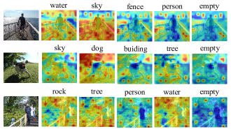
Figure 7: Noisy activations are similar across labels and occur in the empty prompt. Note, “empty” in the last column indicates using an empty string as the label.

The second evidence is the improvements after removing these redundant features. Specifically, we remove the redundant features as Sec. 4.3. Then, we evaluate the performance on explainability task and multi-label recognition as Tab. 1. This table suggests the performances are significantly improved for each listed task, which directly prove the removed feat features are redundant and unnecessary. Besides, we can see the noises are obviously mitigated after the removal of redundant features; see Fig. 8.

4.3 CLIP Feature Surgery

This is the second part of CLIP Surgery, which aims to mitigate the problem of noisy activations by removing redundant features. As illustrated in Fig. 7, these noisy activations are common across different categories. Therefore, computing the mean features along the class dimension can be an effective approach to identify redundant features. Additionally, in our observation, some categories are influenced by the high-scoring obvious classes, which may result in false activations. Thus, we give extra emphasis to these obvious classes, when measuring the redundant features.

Next, we present the formulation of the CLIP Feature Surgery technique. To start with, we obtain the multiplied features $\boldsymbol{F}_{m}\in\mathbb{R}^{N_{i}\times N_{t}\times C}$ in Eq. 6, by element-wise multiplication $\odot$ between the expanded image features $\hat{\boldsymbol{F}_{i}}\in\mathbb{R}^{N_{i}\times N_{t}\times C}$ and the expanded text features $\hat{\boldsymbol{F}_{t}}\in\mathbb{R}^{N_{i}\times N_{t}\times C}$. Specifically, we expand $\boldsymbol{F}_{i}$ to $\hat{\boldsymbol{F}_{i}}$ by coping it $N_{t}$ times, and copy $\boldsymbol{F}_{t}$ $N_{i}$ times as $\hat{\boldsymbol{F}_{t}}$. Here, $N_{t}$, $N_{i}$, and $C$ represent the number of text tokens, image tokens, and channels, respectively. And L2 normalization is operated along the channel dimension.

$$\boldsymbol{F}_{m}=\frac{\hat{\boldsymbol{F}_{i}}}{\|\hat{\boldsymbol{F}_{i}}\|_{2}}\odot\frac{\hat{\boldsymbol{F}_{t}}}{\|\hat{\boldsymbol{F}_{t}}\|_{2}}$$ (6)

In addition, to calculate the category weight $\boldsymbol{w}\in\mathbb{R}^{1\times N_{t}}$ to emphasize obvious classes as Eq. 7, we also require the similarity score $\boldsymbol{s}\in\mathbb{R}^{1\times N_{t}}$, which is computed from the feature $\boldsymbol{F}_{c}\in\mathbb{R}^{1\times C}$ of the class token (the original output of CLIP’s image encoder) and the text features $\boldsymbol{F}_{t}\in\mathbb{R}^{N_{t}\times C}$. Where $\tau$ is the logit scale for softmax, $\|\ \|_{2}$ indicates the L2 normalization along $C$ dimension, and weight $w$ is normalized by its mean value.

$$\begin{split}\boldsymbol{w}=&\frac{\boldsymbol{s}}{mean(\boldsymbol{s})},\ s.t.\\ &\boldsymbol{s}=softmax(\frac{\boldsymbol{F}_{c}}{\|\boldsymbol{F}_{c}\|_{2}}\cdot(\frac{\boldsymbol{F}_{t}}{\|\boldsymbol{F}_{t}\|_{2}})^{\top}\cdot\tau)\end{split}$$ (7)

Then we compute the common and redundant features $\boldsymbol{F}_{r}\in\mathbb{R}^{N_{i}\times 1\times C}$ by counting the mean value of multiplied features $\boldsymbol{F}_{m}\in\mathbb{R}^{N_{i}\times N_{t},C}$ in Eq. 6 along the category dimension ($N_{t}$) as Eq. 8. Note, the weight $expand(\boldsymbol{w})\in\mathbb{R}^{N_{i}\times N_{t},C}$ is the expanded from $\boldsymbol{w}$ in Eq. 7 via copying it $N_{t}$ times to be the same as $\boldsymbol{F}_{m}$.

$$\boldsymbol{F}_{r}=mean(\boldsymbol{F}_{m}\odot expand(\boldsymbol{w}))\ .$$ (8)

In the last, we expand redundant features $\boldsymbol{F}_{r}$ to the same shape as multiplied features $\boldsymbol{F}_{m}$,and write the final equation of CLIP Feature Surgery as:

$$\boldsymbol{S}=sum(\boldsymbol{F}_{m}-expand(\boldsymbol{F}_{r}))\ ,$$ (9)

where $\boldsymbol{S}\in\mathbb{R}^{N_{i}\times N_{t}}$ is the map of cosine similarity distance. Within this equation, $\boldsymbol{F}_{m}-expand(\boldsymbol{F}_{r})$ indicates the removal of redundant features. And element-wise multiplication in Eq. 6 with summation along $C$ dimension in this equation is the same as matrix inner production to compute cosine similarity $\boldsymbol{S}$.

Note that Eq. 9 is specifically designed for the explainability task, and the final similarity map is obtained from $\hat{\boldsymbol{M}}=norm(resize(reshape(\boldsymbol{S})))$ (using the same operations as in Equation 1). For multi-label recognition tasks, we only need to replace $\hat{\boldsymbol{F}}_{i}$ in Equation 6 with the original features of the class token $\boldsymbol{F}_{c}\in\mathbb{R}^{1\times C}$ to obtain the cosine similarity distance $\hat{\boldsymbol{S}}\in\mathbb{R}^{1\times N_{t}}$ for multi-label classification. Furthermore, it is worth noting that CLIP Feature Surgery is not applicable to single-label classification or rank-based metrics like F1 score in multi-label classification. This is because $\boldsymbol{F}_{r}$ can be considered as a common bias, which does not affect the ranking of categories within a single image. Instead, it improves mAP of multi-label classification by adjusting the scores and reducing the false alarm rate across images.

5 Experiments

In this section, we first introduce our experimental setups, including datasets, evaluation metrics, and implementation details. Then we highlight the significant improvements in visual explainability that our approach achieves. Furthermore, our experiments demonstrate that downstream tasks, such as open-vocabulary semantic segmentation and open-vocabulary multi-label recognition, also exhibit significant improvements. In the last, we draw the multimodal visualization results for the image-text pairs, with some interesting observations.

5.1 Setup

5.1.1 Datasets

The proposed CLIP Surgery is operated on the inference stage without training, thus we don’t need any training datasets. To evaluate our method, we use the validation split of each dataset. Specifically, for explainability task, we use PASCAL VOC 2012 everingham2010pascal (1,449 images with 20 foregrounds), MS COCO 2017 lin2014microsoft (5,000 images with 80 foregrounds), PASCAL Context mottaghi2014role (5,105 images with 59 classes), and ImageNet-Segmentation-50 gao2022large (ImageNet-S50, 752 images with 50 classes), where single-label, multi-label, object and stuff are included for comprehensive evaluation. We also use the same datasets as the explainability task to evaluate the interactive segmentation task. For open-vocabulary semantic segmentation task, besides PASCAL Context mottaghi2014role , we test our CLIP Surgery on two widely used semantic segmentation datasets: COCO Stuff caesar2018coco (5,000 images with 171 categories) and CityScapes cordts2016cityscapes (500 images with 19 classes). For open-vocabulary multi-label recognition task, we use PASCAL Context mottaghi2014role , and the most used datasets in multi-label classification: NUS-Wide chua2009nus where there are 107,859 images and 81 concepts. Besides, we use image-text pairs in GCC3M dataset sharma2018conceptual for the multimodal visualization task.

5.1.2 Implementation

For explainability task, we set experiments on the official CLIP with 5 backbones, namely ResNet-50, ResNet-101, ViT-B/32, ViT-B/16, ViT-L/14. For ResNets he2016deep , CLIP adds an attention pooling with self-attention in the last layer, and their output size is 7 $\times$ 7 under input resolution 224 (all the datasets are resized to 224 $\times$ 224 without crop or other augmentation). For the output size of ViTs dosovitskiy2020image , it depends on its patch size. Specifically, the output sizes are 7, 14, 16 for ViT-B/32, ViT-B/16, ViT-L/14, respectively. As for the hyperparameters of CLIP Surgery, the depth $d$ in Eq. 5 is set to 7, and softmax scale $\tau$ in Eq. 7 is set to 2. Note, these hyperparameters are not sensitive with small variation of results. For example, on COCO 2017 lin2014microsoft dataset using backbone ViT-B/16, the variation of results at metric mSC is 0.42% for $d\in[1,10]$, and variation for $\tau\in[1,10]$ is 0.12%. As to the textual prompt, we deploy the 85 templates in CLIP for ImageNet deng2009imagenet , and combine templates with the names of categories. Then, we mean the text features along template dimension as the final text features $F_{t}$, and this prompt ensemble is applied to all methods for fair comparison.

For open-vocabulary semantic segmentation, we resize the images of PASCAL Context mottaghi2014role and COCO Stuff caesar2018coco to 512 $\times$ 512, and crop each image of Cityscapes to 8 patches at 512 $\times$ 512 from 2048 $\times$ 1024 without overlap. For fair comparison, all the compared methods use the same backbone ViT-B/16, except grouping methods xu2022groupvit ; luo2022segclip whose backbones are specially designed. Note, the original ReCo shin2022reco uses ResNet50x16 which is much larger than ViT-B/16, and the implemented results based on ViT-B/16 are from the official code. Since ViL-Seg liu2022open is not released, we report its results from the paper. And we reproduce the results of MaskCLIP zhou2022extract at the same settings as ours, without its post-processing methods, for fair comparison with other works. For open-vocabulary multi-label recognition, we take the prediction from the original path (the same as original CLIP at input size 224), and apply feature surgery to replace the softmax operation of CLIP. For other CLIP-based zero-shot methods sun2022dualcoop ; xu2022dual ; he2022open , we report their results from the papers. Besides, we implement TaI-DPT guo2022texts from the official code as a baseline, and apply the feature surgery on its predictions to verify the complementarity of our method.

For the interactive segmentation, we convert text to points for the Segment Anything Model (SAM) kirillov2023segment . It helps to replace the cost of manual labeling and avoids bad performance of SAM using text prompt only. Specifically, we pick points whose scores are higher than 0.8 from the similarity map, and take the same number of points ranked last as background points. Note, there is only one text prompt for SAM instead of multiple texts. Thus, we implement the feature surgery via the redundant feature $\boldsymbol{F}_{empty}$ from text features of an empty string to replace $expand(\boldsymbol{F}_{r})$ in Eq. 9. This situation is the same to multimodal visualization, where the whole sentence is used as a text label without other categories. And we use the string “[start][end]” (start flag and end flag, respectively) to extract redundant feature.

5.1.3 Evaluation Metrics

We use the most common evaluation metrics for open-vocabulary segmentation and multi-label recognition. They are mean Intersection over Union (mIoU) and mean Average Precision (mAP) for segmentation and recognition, respectively. For interactive segmentation, we use accuracy (Acc) to evaluate the correctness of point prompts from explainability methods. And we use mIoU to evaluate each positive label independently. We will not introduce the above metrics in detail, because they are widely used with open formulas. We mainly introduce the metrics in li2022exploring for explainability. Specifically, the mIoU is also used to measure the visualization quality. While each positive label is evaluated independently with a grid search threshold to identify the foreground. Since explainability methods are usually evaluated on single label, and the searched threshold avoids manual threshold when identifying the foreground.

The new metric for explainability is mean Score Contrast (mSC), which refers to the score difference between foregrounds and backgrounds, ranging from -100% to 100%. This metric is able to reflect the problem of opposite visualization when the value is lower than 0, but mIoU cannot. Besides, mSC measures the difference of scores, while mIoU measures the mask without information of confidence. Thus, higher mSC indicates larger color contrast and better visualization quality. We give the formula definition as:

$$mSC=m_{c}(m_{s}(S_{f}-S_{b}))\ ,$$ (10)

where $S_{f},S_{b}$ indicates the mean foreground score and background score for each label, and $m_{c},m_{s}$ compute the mean values along dimensions of classes and samples, respectively.

Table 1: Ablation study of CLIP Surgery. “no” is the original CLIP, “Archi.” indicates the CLIP Architecture Surgery and “Feat.” means the CLIP Feature Surgery. Note, mSC lower than 0 suggests scores of background is higher than foreground, and “Archi.” greatly improves this metric. Besides, “Feat.” contributes to both explainability task and open-vocabulary multi-label recognition task.

	Explainability		Multi-label
CLIP Surgery	mSC (%) $\uparrow$	mIoU (%) $\uparrow$	mAP (%) $\uparrow$
no	-16.73	15.76	47.09
Archi.	31.15	43.47	47.09
Archi. + Feat.	34.32	46.28	52.61

5.2 Results of Explainability

5.2.1 Ablation Study

We set ablation studies on Pascal Context dataset mottaghi2014role with backbone ViT-B/16 of CLIP. The first ablation experiment is listed in Tab. 1 about two parts of CLIP Surgery. From metric mSC, we can see CLIP Architecture Surgery greatly improves the explainability by 47.88%, and CLIP Feature Surgery further boosts it by 3.17%. For multi-label recognition task, the features are from the original path, thus the mAP is not changed. While CLIP Feature Surgery significantly improves it by 5.52%. From these numbers, we can see the feature surgery improves both explainability task and multi-label recognition task, which indicates the removed features of feature surgery are harmful, and support the claim of redundant feature in Sec. 4.2.

Table 2: Ablation study about multi-layers, dual paths and FFN. “Last” indicates the CLIP Architecture Surgery is only applied on the last layer, and “Multi” means applying to multiple layers. “Dual” is the proposed dual paths. Besides, “FFN” indicates only feed-forward networks are used, and “Attn” only takes self-attentions.

Last	Multi	Dual	FFN	Attn	mSC (%) $\uparrow$
✓					29.13
	✓				-7.73
	✓	✓			32.30
	✓	✓	✓		-4.28
	✓	✓		✓	34.32

Table 3: Results comparison between “CLIP” and “Ours” on four datasets and five backbones. Metric mIoU (%) measures the mask-level explainability for positive labels. And mSC (%) in Eq. 10 ranges from -100% to 100%, reflecting the score contrast between foreground and background, where the value lower than 0 indicates the model prefers the background more. Note, “$\Delta$” indicates our average improvements over five backbones.

		ImageNet-S50		VOC 2012		PASCAL Context		COCO 2017
Method	Network	mIoU $\uparrow$	mSC $\uparrow$	mIoU $\uparrow$	mSC $\uparrow$	mIoU $\uparrow$	mSC $\uparrow$	mIoU $\uparrow$	mSC $\uparrow$
CLIP	ResNet50	28.18	-26.50	17.78	-27.88	16.98	-14.02	10.53	-19.17
Ours	ResNet50	66.05	43.28	53.85	44.60	38.50	32.44	29.24	33.80
1-10[0.5pt/5pt] CLIP	ResNet101	28.17	-23.30	18.06	-23.48	17.52	-9.90	10.66	-17.31
Ours	ResNet101	65.51	43.22	52.51	44.07	38.03	32.21	29.89	35.50
1-10[0.5pt/5pt] CLIP	ViT-B/32	28.05	-21.86	17.56	-24.06	16.37	-17.68	10.15	-21.02
Ours	ViT-B/32	59.24	36.72	51.14	41.15	40.10	32.90	29.22	31.35
1-10[0.5pt/5pt] CLIP	ViT-B/16	27.87	-18.84	17.36	-19.86	15.76	-16.73	9.74	-23.37
Ours	ViT-B/16	62.41	36.50	55.78	41.64	46.28	34.32	35.23	35.43
1-10[0.5pt/5pt] CLIP	ViT-L/14	27.89	-18.34	17.24	-24.42	15.62	-20.26	9.64	-27.51
Ours	ViT-L/14	61.72	28.25	54.47	34.89	42.71	28.11	37.67	32.54
$\Delta$	-	34.96	59.36	35.95	65.21	24.67	47.72	22.11	55.40

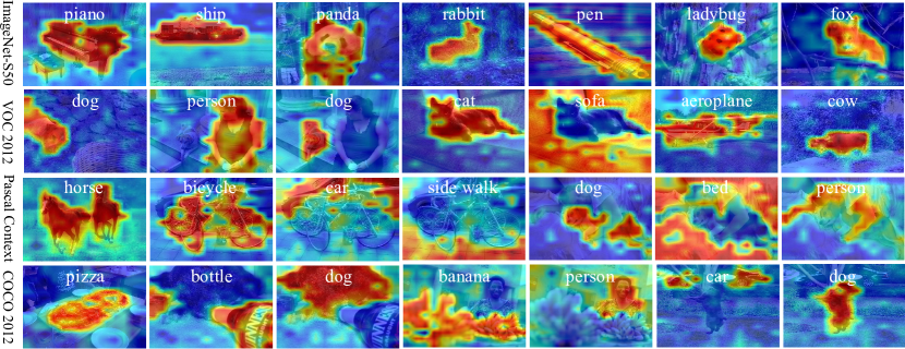
Figure 8: Our CLIP Surgery solves the explainability problems, and provides good visualizations on varied datasets.

The second ablation study is listed in Tab. 2 about multiple layer, dual paths, and FFN. In this table, the first row indicates the mSC is 29.13% when the last q-k self-attention (Eq. 2) is replaced by new self-attention (Eq. 3). But the result is merely -7.73% when the new self-attention is applied to multiple layers. It’s owing to the modified outputs of new self-attention, which influence next layers one by one, and thus lead to model crash. This situation is corrected after introducing the proposed dual paths. It keeps the input of each block the same, thus stabilizes the model at mSC 32.30% (40.03% higher than the original single path). For the FFN, it cannot be used solely without self-attentions, while the new self-attention performs better without FFN (-4.28% vs. 34.32%). This result is corresponding to Fig. 5, where the features of FFN are near to negative labels than positive labels. From this table, we find the dual paths is essential for multi-layers, and using new self-attention only achieves the best result at 34.32%.

Table 4: Results compared with previous state-of-the-art explainability methods. CLIP indicates the similarity map of CLIP. “†” means the model requires extra fine-tuning, and “$\star$” indicates that back-propagations are required for each label at lower efficiency. Note, mIoU (%) measures the mean intersection over union for positive labels, and mSC indicates the mean score contrast in Eq. 10. All methods use the backbone ViT-B/16 at the same resolution and prompt for fair comparison.

	ImageNet-S50		VOC 2012		PASCAL Context		COCO 2017
Method	mIoU $\uparrow$	mSC $\uparrow$	mIoU $\uparrow$	mSC $\uparrow$	mIoU $\uparrow$	mSC $\uparrow$	mIoU $\uparrow$	mSC $\uparrow$
CLIP radford2021learning	27.87	-18.84	17.36	-19.86	15.76	-16.73	9.74	-23.37
Grad-CAM⋆ selvaraju2017grad	28.59	-11.05	17.90	-14.51	16.04	-14.68	9.89	-18.91
pLRP⋆ lapuschkin2019unmasking	46.76	10.33	31.73	8.88	25.61	6.24	21.06	11.22
Bi-Modal⋆ chefer2021generic	43.37	6.77	30.64	6.76	24.31	3.95	18.33	7.99
gScoreCAM⋆ chen2022gscorecam	24.75	7.47	11.33	1.59	13.26	0.35	13.59	4.45
RCLIP li2022exploring	48.00	16.14	37.36	18.51	33.25	18.21	26.12	22.41
ECLIP†li2022exploring	58.59	26.32	48.46	28.83	30.34	14.43	24.67	18.95
CLIP Surgery (Ours)	62.41	36.50	55.78	41.64	46.28	34.32	35.23	35.43

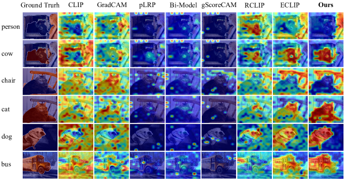
Figure 9: Visual comparison between our CLIP Surgery with state-of-the-art explainability methods on VOC 2012 everingham2010pascal . Note the foregrounds are colored in red, and the backbone is ViT-B/16. Our visualization quality is much better than other methods, without any fine-tuning in ECLIP li2022exploring or back-propagation in GradCAM selvaraju2017grad , pLRP lapuschkin2019unmasking , Bi-Modal chefer2021generic and gScoreCAM chen2022gscorecam .

5.2.2 Effectiveness of CLIP Surgery

Table 3 shows a comparison between the proposed CLIP Surgery and the original CLIP model. The comparison is performed on four datasets using five backbones. Our results consistently outperform the CLIP baselines in each setting, with significant improvements. On average, our method achieves a higher mIoU than CLIP by 22.11% to 35.95%, and a higher mSC by 47.72% to 65.21%. Notably, while the mSC of CLIP is lower than 0, indicating that the model tends to favor the background over the foreground, our CLIP Surgery corrects this issue, yielding results far above 0. These results provide strong evidence for the effectiveness of our proposed method, which is applicable to both ResNets he2016deep and ViTs dosovitskiy2020image .

Additionally, we present visualization results for different datasets in Fig. 8. The visualizations demonstrate that our proposed method effectively addresses the two discussed problems: opposite visualization and noisy activations. Notably, the proposed method enables us to produce clear and interpretable visualizations based solely on the original CLIP, without any additional training or complex back-propagation.

5.2.3 Compassion with Previous Works

In this part, we compare the proposed CLIP Surgery with previous explainability works, including similarity map of original CLIP, Grad-CAM selvaraju2017grad for CNN, pLRP lapuschkin2019unmasking implemented by chefer2021transformer for multiple layers, Bi-Modal chefer2021generic based on ViT for multiple modalities, and explainability methods li2022exploring ; chen2022gscorecam for CLIP. We compare our method with them at the same backbone, ViT-B/16, and implement them from the official codebases. We list the results in Table 4. From this table, our CLIP Surgery archives the best performances on all datasets and metrics, also beyond other methods at large margins. The second place is ECLIP li2022exploring where the pooling is replaced with extra training, while our CLIP Surgery still surpasses it by max gains at 15.94% mIoU and 19.89% mSC without any training. Except our method, RCLIP li2022exploring ranks first in the methods without extra training, and our results are significantly higher than it by 18.42% at mIoU and 23.13% at mSC. As for rest methods, their performances gap compared with ours are larger. Within them, Grad-CAM selvaraju2017grad is similar to CLIP, showing the problem of opposite visualization. Besides, gScoreCAM chen2022gscorecam is designed for CLIP, but its results are not better than pLRP lapuschkin2019unmasking and Bi-Modal chefer2021generic for ViT, and we analyze it in the next table.

Table 5: Limitation of output size. Most methods except ours show worse results for higher output size, where the mIoU difference between ViT-B/16 (side 14) and ViT-B/32 (side 7) is lower than 0. Positive results are marked in bold.

Method	VOC 2012	PASCAL Context
Grad-CAM selvaraju2017grad	-0.93	-0.72
pLRP lapuschkin2019unmasking	-7.15	-4.27
Bi-Modal chefer2021generic	-3.53	-2.04
gScoreCAM chen2022gscorecam	-11.98	-8.14
RCLIP li2022exploring	-3.11	2.51
ECLIP li2022exploring	-1.31	-7.64
CLIP Surgery	4.64	1.24

Table 6: Results compared with state-of-the-art methods of open-vocabulary semantic segmentation on three datasets. All the method use the same backbone ViT-B/16 without post-processing or self-training for fair comparison. “Weights” indicate the initial weights. Note, the evaluation metric is mIoU (%).

Method	Weights	Training	Core Idea	PASCAL Context	COCO Stuff	Cityscapes
ViL-Seg liu2022open	CLIP	yes	contrasting and clustering	16.3	16.4	-
ReCo shin2022reco	CLIP	yes	co-segmentation with retrieval	22.3	14.8	21.1
GroupViT xu2022groupvit	scratch	yes	tokens grouping	22.4	13.3	12.4
Seg-CLIP luo2022segclip	CLIP	yes	grouping with learnable centers	24.7	-	-
MaskCLIP zhou2022extract	CLIP	no	modify attention pooling	22.4	15.3	22.7
CLIP Surgery	CLIP	no	improve explainability	29.3	21.9	31.4

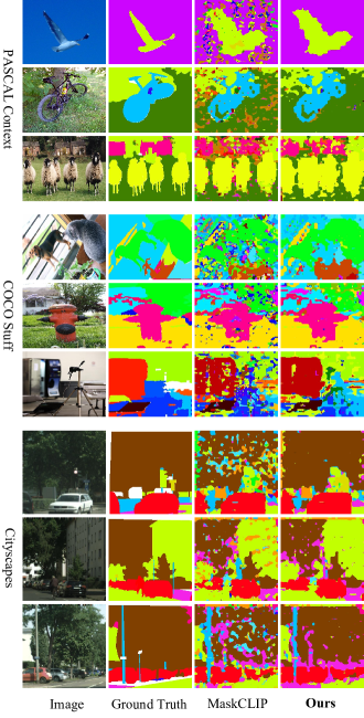
Figure 10: Visual comparison of open-vocabulary semantic segmentation. We compare our CLIP Surgery with state-of-the-art methods MaskCLIP zhou2022extract on PASCAL Context mottaghi2014role , COCO stuff caesar2018coco and patch of Cityscapes cordts2016cityscapes , respectively.

We observe another problem from Tab. 4, where the results of gScoreCAM chen2022gscorecam are bad, even it’s designed for CLIP. One reason is that it’s not suitable for ViT, besides, it’s owning to the limitation of output size. As shown in Tab. 5, most methods meet a performance drop when the output size is scaled up from 7 (ViT-B/32) to 14 (ViT-B/16). Within these methods, gScoreCAM is the most obvious method where the performances drop most for higher output size. It means it works better in lower output size, and it’s highly limited at output size. This problem is easy to explain, because the min side of highlight is $\frac{1}{7}$ of ViT-B/32, and it reduces half for ViT-B/16. Thus, methods which focus on local region highlight less area with worse results. While our method is not limited by the output size or patch size, and our results are higher when the model is scaled up. This finding suggests our method is applicable to tasks requiring dense predictions like segmentation.

In addition to the quantitative comparison, we also present a visual comparison in Fig. 9. The results show that our CLIP Surgery provides better quality visualizations compared to existing explainability methods, without problems of opposite visualization. Furthermore, our method produces fewer noisy activations than methods like pLRP lapuschkin2019unmasking , Bi-Modal chefer2021generic , gScoreCAM chen2022gscorecam . Also, our method shows more obvious score contrast than RCLIP and ECLIP li2022exploring at better visualization quality. All the above improvements enhance the model’s visual explainability and make it more credible.

5.3 Results of Open-Vocabulary Semantic Segmentation

We find that the high-quality visualization results produced by our CLIP Surgery method are well-suited for the task of semantic segmentation. In particular, our method is not limited by the output size, as demonstrated in Tab. 5, allowing us to scale up the model for dense predictions to segment objects and stuffs. As described in Sec. 5.1.2, we set the input size to 512 $\times$ 512 for dense predictions, and apply an argmax operation across the category dimension to generate the segmentation output. Despite requiring no extra training, our method performs exceptionally well, and even surpasses existing open-vocabulary segmentation methods that require extra training, as shown in Tab. 6. Specifically, our CLIP Surgery achieves the best results on three datasets, surpassing the second-best method by 4.6%, 5.5%, and 8.7%, respectively. Besides the noticeable effectiveness, we list the differences of core ideas among methods, and CLIP Surgery is the prior work to introduce explainability into open-vocabulary segmentation task with highly novelty.

We also list other works about semantic segmentation with CLIP in the related work (Sec. 2.2). While some works require partial mask annotations bucher2019zero ; xu2021simple , additional supervised proposal network zhong2022regionclip , extra supervision zhang2022glipv2 , or extra saliency model shin2022namedmask . Thus, we do not compare them in Tab. 6. Besides, MaskCLIP zhou2022extract is the most similar work to ours, as it requires no training too. And we recap the differences: (1) Our goal is to introduce better explainability into segmentation with in-depth analyses, while MaskCLIP is designed for segmentation. (2) In the aspect of operation, we reform the self-attention, while it deletes self-attention and keep feature of “value”. (3) We propose the dual paths to apply new self-attention for multiple layers, while the target of MaskCLIP is only the last self-attention layer. Compared to other methods, our CLIP Surgery is highly practical as it does not require any fine-tuning, and has demonstrated superior effectiveness.

Then We perform a visual comparison between our method and previous state-of-the-art method MaskCLIP zhou2022extract , as shown in Fig. 10. The visualizations across datasets demonstrate the effectiveness of our approach in handling complex scenes without the need for pixel-level annotation. Our explainability method is capable of transferring well to the segmentation task, as evidenced by these results.

5.4 Results of Open-Vocabulary Multi-Label Recognition

Table 7: Open-vocabulary multi-label recognition results with different activation operations. “None” indicates original cosine distance, and “Ours” is the proposed CLIP Feature Surgery. The evaluation metric is mAP (%).

Method	PASCAL Context	NUS-Wide
ResNet-50
1-3[0.5pt/5pt] None	36.91	32.75
Sigmoid	36.52	32.24
Softmax	43.90	35.58
Ours	47.35	39.99
ViT-B/16
1-3[0.5pt/5pt] None	47.09	35.58
Sigmoid	47.09	40.39
Softmax	49.40	42.85
Ours	52.61	47.19

Table 8: Results compared with state-of-the-art methods about CLIP-based multi-label recognition on NUS-Wide dataset chua2009nus . Our method is complementary to zero-shot methods, which require fine-tuning on seen categories.

Method	Network	Fine-tuning	mAP (%)
CLIP radford2021learning	ResNet-50	no	35.58
Ours	ResNet-50	no	39.99
DualModal xu2022dual	ViT-B/32	yes	36.56
MKT he2022open	ViT-B/16	yes	37.6
DualCoOp sun2022dualcoop	ResNet-50	yes	43.6
TaI-DPT guo2022texts	ResNet-50	yes	44.99
TaI-DPT + Ours	ResNet-50	yes	48.28

For multi-label recognition based on CLIP, we firstly emphasize the importance of activation function and the effectiveness of our method. Unlike previous multi-label recognition methods supervised by fully supervisions, CLIP is sensitive to the final activation function to generate final scores, as shown in Tab. 7. The results of original cosine distance “None” are similar to performances of sigmoid, which are obviously lower than softmax. Because, the contrastive loss of CLIP corresponds to softmax. For our method, we apply the CLIP feature surgery via replacing features of image tokens $\hat{F}_{i}$ to features of class token $F_{c}$ as described in the last paragraph of Sec. 4.3. It removes the redundant features with significant improvements on the evaluated datasets, where the gains at backbone ResNet-50 are 3.45%, 4.41% compared with the second on PASCAL Context mottaghi2014role and NUS-Wide chua2009nus , respectively. Also, the improvement is over 10% compared with the original logit “None” on PASCAL Context. All above results show the noticeable effectiveness of our approach.

Then, we compare our method with existing CLIP-based zero-shot multi-label recognition in Tab. 8. Our method is 4.41% higher than original CLIP without fine-tuning, and has already beyond some methods requiring fine-tuning. After combining with TaI-DPT guo2022texts , we achieve new state-of-the-art result on NUS-Wide chua2009nus at mAP 48.28%, which is 3.29% higher than the implemented TaI-DPT from its official code. These results suggest our method is effective, also it’s complementary to methods at zero-shot settings which requiring fine-tuning on seen categories.

5.5 Application on Open-Vocabulary Interactive Segmentation

5.5.1 Motivation and Advantages

Interactive segmentation boykov2001interactive ; rother2004grabcut ; lempitsky2009image is a classical computer vision task that involves segmenting a target object from an image with user guidance in the form of points, scribbles, or boxes during the inference phase. With the advent of large vision models, a recent work called the Segment Anything Model (SAM) kirillov2023segment has made significant progress in enabling interactive segmentation via text prompts in an open-vocabulary manner. However, the SAM model performs poorly with text prompts alone, and the authors suggest combining text with manual points for better results. Our motivation is to replace the need for manual points entirely by using CLIP Surgery with text-only inputs. Our proposed method provides pixel-level results from text input, which can be readily converted to point prompts for the SAM model. Specifically, we select foreground points ranked ahead in the similarity map, and use the same number of points ranked last as background points.

When compared to other explainability methods, our CLIP Surgery offers two distinct advantages in converting text to points: (1) We have successfully mitigated the impact of noisy activations. As a result, the top points generated by our method are more reliable than those produced by other methods. (2) Our method is not limited by resolution, as demonstrated in Table 5. This enables us to increase resolution as needed to achieve better segmentation results.

Our solution offers several advantages over other prompt formats in SAM. (1) Our method requires text input only, without the annotation cost of manual points suggested in the paper of SAM (specifically, figure 12). (2) Point prompts are superior to mask prompts, because SAM’s mask prompt is designed for its own output logits. This means that the generated points are more suitable than masks from another model. (3) Text to points is more readily achievable than the solution of text to boxes, because we only need CLIP without any fine-tuning. In contrast, open-vocabulary detection methods generate boxes requiring fine-tuning du2022learning , and additional supervisions zhang2022glipv2 or models like proposal networks zhong2022regionclip are usually needed.

5.5.2 Results and Visualization

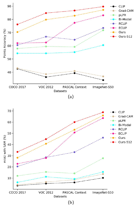
Figure 11: Comparison of points accuracy (a) and mIoU with SAM kirillov2023segment among explainability methods on four datasets. Note, “Ours-512” indicates the input size of our CLIP Surgery is 512, and rest results use input size 224.

We focus to compare with other explainability methods in the solution of text to points. For all methods, we use the ViT-B/16 of CLIP as the backbone, with an input size of 224. Then, we select points with scores higher than 0.8 as positives, and use the same number of negatives ranked last as input prompts for the SAM. The accuracy of points and the mIoU after the SAM processing are plotted in Fig. 11. Our method outperforms others in terms of both points accuracy and mIoU with SAM all four datasets. Specifically, We achieve points accuracies close to 90% on some datasets, and the mIoU on ImageNet-S50 is approximately 70%. Note that the mIoU is evaluated independently on each positive label.

Table 9: Ablation study on PASCAL Context dataset mottaghi2014role . ^⋆ indicates higher resolution (512) further improves the results.

Threshold	Point Accuracy (%)	mIoU (%)
0.6	73.16	36.85
0.65	74.86	38.12
0.7	76.59	39.12
0.75	78.26	39.86
0.8	79.83	40.70
0.85	81.13	40.50
0.9	82.44	39.60
0.95	83.29	37.65
0.8⋆	84.75	44.75

We have also included the results of our ablation study in Table 9. The table reveals that having a higher threshold results in higher points accuracy. However, a moderate threshold of 0.8 performs the best because a lower threshold introduces more points and maintains higher recall. Furthermore, increasing the input resolution significantly improves accuracy and mIoU.

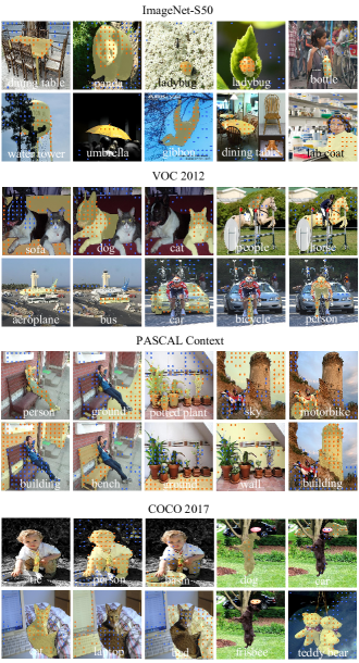
Figure 12: Visualization of SAM kirillov2023segment (yellow mask) using point prompts from our CLIP Surgery. The orange points indicate the foregrounds and blue points mean the backgrounds.

We have also included visualizations of our results in Fig. 12. These visualizations showcase the predicted mask from SAM as well as the points prompt generated by our CLIP Surgery. Notably, we use the ViT-B/16 backbone at an input size of 512. The visualization results demonstrate that SAM guided by CLIP Surgery performs better than the similarity map or semantic segmentation results. In particular, the mask generated after SAM processing is impressive at the boundary with very few noisy pixels, resulting in a higher visual quality. Additionally, the points generated by our CLIP Surgery are accurate, indicating that our method is applicable and effective.

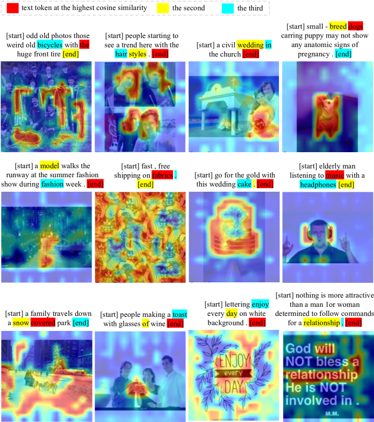
Figure 13: Multimodal visualization to explain the image-text pairs used in the training process of CLIP. The visual explainability results are from the proposed CLIP Surgery, and textual explainability results are based on the cosine distance of each text token. [start] indicates the start text token and [end] means the end text token. Note, we mark the text token at the highest cosine similarly in red, then draw the second in yellow and blue for the third.

5.6 Multimodal Visualization Results

Besides above visualization results on image modality for varied tasks, we also explain the learning process of CLIP by the multimodal visualization. Specifically, we visualize the image-text pairs during training, where the whole sentence is used as a textual label for visual explanation. At the same time, we show the top text tokens whose scores are ranked in front. For the implementation, we use image-text pairs (training data) from the GCC3M dataset sharma2018conceptual , since the training data of CLIP is private and not available. Then we draw the similarity map via our CLIP Surgery method, and mark the high response text tokens. Specifically, the feature of class token $\boldsymbol{F_{c}}$ is used to compute similarity scores for each text token, and the text at max similarity is served for the generation of similarity map with image tokens $\boldsymbol{F_{i}}$. Note, there is only one sentence instead of multiple texts, thus we implement the feature surgery via the redundant feature $\boldsymbol{F}_{empty}$ from text features of an empty sentence ([start][end]) to replace $expand(\boldsymbol{F}_{r})$ in Eq. 9. Besides. the backbone is ViT-B/16 at input resolution 224. Based on above implementation details, we draw multimodal visualization results as Fig. 13.

From these multimodal visualization results, we observed some interesting phenomenons. For the visual results, we summarize two points: (1) Not all the objects or stuffs are highlighted in the image, because only the text token at the highest cosine similarity is picked for training (red texts in Fig. 13). Thus, we believe CLIP learns partial context from one image. (2) CLIP is able to recognize the texts from an image in some extent, as shown in the last two images of Fig. 13. Since the highlights are corresponded with text tokens (e.g., day, enjoy, relationship). For the textual visualization results, there are two findings: (1) The end token is the most common activated text token, and some non-object words are at high response too (e.g., “in”, “.”, “of”). It means the text encoder of CLIP embeds the information of whole sentences in certain words. (2) The object-based words also occurs frequently with corresponding salient objects in the image. While their cosine similarities often ranks second or third behind the end token “[end]”. These findings are interesting, also they reveal some characteristics of image-text pairs of CLIP, thus provides potential value to further improvement of CLIP’s training process.

6 Conclusion

In this study, we investigate two observations related to the explainability of CLIP, namely the opposite visualization and the noisy activations. We identify that the erroneous parameters in self-attention tend to focus on opposite semantic regions, leading to the problem of opposite visualization. Our findings also reveal that self-attentions in CLIP exhibit better explainability than feed-forward networks. Consequently, we proposed the CLIP Surgery method, which involves merging multiple v-v self-attentions with dual paths, to address the problem of opposite visualization. Furthermore, we find that the presence of noisy activations in CLIP is attributed to redundant features. To address this issue, we propose the CLIP Surgery on the output features, which involves removing the common but redundant features. Our CLIP Surgery effectively solves these problems, making significant improvements in visual explainability. Moreover, we demonstrate that the proposed method could be extended to open-vocabulary semantic segmentation, interactive segmentation, and multi-label recognition tasks with significant improvements. Also, it’s able to explain the image-text pairs used in CLIP’s training process, thus provides some new insights. Overall, the proposed CLIP Surgery offers a promising solution for better explainability of CLIP, with significant enhancements in downstream open-vocabulary tasks.

Data availability All datasets analyzed during the current study are publicly available.

References

- [1] Zeynep Akata, Florent Perronnin, Zaid Harchaoui, and Cordelia Schmid. Label-embedding for image classification. IEEE transactions on pattern analysis and machine intelligence, 38(7):1425–1438, 2015.
- [2] Omer Bar-Tal, Dolev Ofri-Amar, Rafail Fridman, Yoni Kasten, and Tali Dekel. Text2live: Text-driven layered image and video editing. In Computer Vision–ECCV 2022: 17th European Conference, Tel Aviv, Israel, October 23–27, 2022, Proceedings, Part XV, pages 707–723. Springer, 2022.
- [3] Avi Ben-Cohen, Nadav Zamir, Emanuel Ben-Baruch, Itamar Friedman, and Lihi Zelnik-Manor. Semantic diversity learning for zero-shot multi-label classification. In Proceedings of the IEEE/CVF International Conference on Computer Vision, pages 640–650, 2021.
- [4] Yuri Y Boykov and M-P Jolly. Interactive graph cuts for optimal boundary & region segmentation of objects in nd images. In Proceedings eighth IEEE international conference on computer vision. ICCV 2001, volume 1, pages 105–112. IEEE, 2001.
- [5] Maxime Bucher, Tuan-Hung Vu, Matthieu Cord, and Patrick Pérez. Zero-shot semantic segmentation. Advances in Neural Information Processing Systems, 32, 2019.
- [6] Holger Caesar, Jasper Uijlings, and Vittorio Ferrari. Coco-stuff: Thing and stuff classes in context. In Proceedings of the IEEE conference on computer vision and pattern recognition, pages 1209–1218, 2018.
- [7] Aditya Chattopadhay, Anirban Sarkar, Prantik Howlader, and Vineeth N Balasubramanian. Grad-cam++: Generalized gradient-based visual explanations for deep convolutional networks. In 2018 IEEE winter conference on applications of computer vision (WACV), pages 839–847. IEEE, 2018.
- [8] Hila Chefer, Shir Gur, and Lior Wolf. Generic attention-model explainability for interpreting bi-modal and encoder-decoder transformers. In Proceedings of the IEEE/CVF International Conference on Computer Vision, pages 397–406, 2021.
- [9] Hila Chefer, Shir Gur, and Lior Wolf. Transformer interpretability beyond attention visualization. In Proceedings of the IEEE/CVF Conference on Computer Vision and Pattern Recognition, pages 782–791, 2021.
- [10] Peijie Chen, Qi Li, Saad Biaz, Trung Bui, and Anh Nguyen. gscorecam: What objects is clip looking at? In Proceedings of the Asian Conference on Computer Vision, pages 1959–1975, 2022.
- [11] Yunpeng Chen, Jianan Li, Huaxin Xiao, Xiaojie Jin, Shuicheng Yan, and Jiashi Feng. Dual path networks. Advances in neural information processing systems, 30, 2017.
- [12] Tat-Seng Chua, Jinhui Tang, Richang Hong, Haojie Li, Zhiping Luo, and Yantao Zheng. Nus-wide: a real-world web image database from national university of singapore. In Proceedings of the ACM international conference on image and video retrieval, pages 1–9, 2009.
- [13] Marcos V Conde and Kerem Turgutlu. Clip-art: contrastive pre-training for fine-grained art classification. In Proceedings of the IEEE/CVF Conference on Computer Vision and Pattern Recognition, pages 3956–3960, 2021.
- [14] Marius Cordts, Mohamed Omran, Sebastian Ramos, Timo Rehfeld, Markus Enzweiler, Rodrigo Benenson, Uwe Franke, Stefan Roth, and Bernt Schiele. The cityscapes dataset for semantic urban scene understanding. In Proceedings of the IEEE conference on computer vision and pattern recognition, pages 3213–3223, 2016.
- [15] Jia Deng, Wei Dong, Richard Socher, Li-Jia Li, Kai Li, and Li Fei-Fei. Imagenet: A large-scale hierarchical image database. In 2009 IEEE conference on computer vision and pattern recognition, pages 248–255. Ieee, 2009.
- [16] Alexey Dosovitskiy, Lucas Beyer, Alexander Kolesnikov, Dirk Weissenborn, Xiaohua Zhai, Thomas Unterthiner, Mostafa Dehghani, Matthias Minderer, Georg Heigold, Sylvain Gelly, et al. An image is worth 16x16 words: Transformers for image recognition at scale. arXiv preprint arXiv:2010.11929, 2020.
- [17] Yu Du, Fangyun Wei, Zihe Zhang, Miaojing Shi, Yue Gao, and Guoqi Li. Learning to prompt for open-vocabulary object detection with vision-language model. In Proceedings of the IEEE/CVF Conference on Computer Vision and Pattern Recognition, pages 14084–14093, 2022.
- [18] Sepideh Esmaeilpour, Bing Liu, Eric Robertson, and Lei Shu. Zero-shot open set detection by extending clip. arXiv preprint arXiv:2109.02748, 2021.
- [19] Mark Everingham, Luc Van Gool, Christopher KI Williams, John Winn, and Andrew Zisserman. The pascal visual object classes (voc) challenge. International journal of computer vision, 88(2):303–338, 2010.
- [20] Shanghua Gao, Zhong-Yu Li, Ming-Hsuan Yang, Ming-Ming Cheng, Junwei Han, and Philip Torr. Large-scale unsupervised semantic segmentation. IEEE Transactions on Pattern Analysis and Machine Intelligence, 2022.
- [21] Wei Gao, Fang Wan, Xingjia Pan, Zhiliang Peng, Qi Tian, Zhenjun Han, Bolei Zhou, and Qixiang Ye. Ts-cam: Token semantic coupled attention map for weakly supervised object localization. In Proceedings of the IEEE/CVF International Conference on Computer Vision, pages 2886–2895, 2021.
- [22] Gabriel Goh, Nick Cammarata, Chelsea Voss, Shan Carter, Michael Petrov, Ludwig Schubert, Alec Radford, and Chris Olah. Multimodal neurons in artificial neural networks. Distill, 6(3):e30, 2021.
- [23] Xiuye Gu, Tsung-Yi Lin, Weicheng Kuo, and Yin Cui. Open-vocabulary object detection via vision and language knowledge distillation. arXiv preprint arXiv:2104.13921, 2021.
- [24] Zixian Guo, Bowen Dong, Zhilong Ji, Jinfeng Bai, Yiwen Guo, and Wangmeng Zuo. Texts as images in prompt tuning for multi-label image recognition. arXiv preprint arXiv:2211.12739, 2022.
- [25] Kaiming He, Xiangyu Zhang, Shaoqing Ren, and Jian Sun. Deep residual learning for image recognition. In Proceedings of the IEEE conference on computer vision and pattern recognition, pages 770–778, 2016.
- [26] Sunan He, Taian Guo, Tao Dai, Ruizhi Qiao, Bo Ren, and Shu-Tao Xia. Open-vocabulary multi-label classification via multi-modal knowledge transfer. arXiv preprint arXiv:2207.01887, 2022.
- [27] Alexander Kirillov, Eric Mintun, Nikhila Ravi, Hanzi Mao, Chloe Rolland, Laura Gustafson, Tete Xiao, Spencer Whitehead, Alexander C Berg, Wan-Yen Lo, et al. Segment anything. arXiv preprint arXiv:2304.02643, 2023.
- [28] Sebastian Lapuschkin, Stephan Wäldchen, Alexander Binder, Grégoire Montavon, Wojciech Samek, and Klaus-Robert Müller. Unmasking clever hans predictors and assessing what machines really learn. Nature communications, 10(1):1096, 2019.
- [29] Victor Lempitsky, Pushmeet Kohli, Carsten Rother, and Toby Sharp. Image segmentation with a bounding box prior. In 2009 IEEE 12th international conference on computer vision, pages 277–284. IEEE, 2009.
- [30] Yi Li, Zhanghui Kuang, Liyang Liu, Yimin Chen, and Wayne Zhang. Pseudo-mask matters in weakly-supervised semantic segmentation. In Proceedings of the IEEE/CVF International Conference on Computer Vision, pages 6964–6973, 2021.
- [31] Yi Li, Hualiang Wang, Yiqun Duan, Hang Xu, and Xiaomeng Li. Exploring visual interpretability for contrastive language-image pre-training. arXiv preprint arXiv:2209.07046, 2022.
- [32] Tsung-Yi Lin, Michael Maire, Serge Belongie, James Hays, Pietro Perona, Deva Ramanan, Piotr Dollár, and C Lawrence Zitnick. Microsoft coco: Common objects in context. In European conference on computer vision, pages 740–755. Springer, 2014.
- [33] Quande Liu, Youpeng Wen, Jianhua Han, Chunjing Xu, Hang Xu, and Xiaodan Liang. Open-world semantic segmentation via contrasting and clustering vision-language embedding. In Computer Vision–ECCV 2022: 17th European Conference, Tel Aviv, Israel, October 23–27, 2022, Proceedings, Part XX, pages 275–292. Springer, 2022.
- [34] Huaishao Luo, Junwei Bao, Youzheng Wu, Xiaodong He, and Tianrui Li. Segclip: Patch aggregation with learnable centers for open-vocabulary semantic segmentation. arXiv preprint arXiv:2211.14813, 2022.
- [35] Roozbeh Mottaghi, Xianjie Chen, Xiaobai Liu, Nam-Gyu Cho, Seong-Whan Lee, Sanja Fidler, Raquel Urtasun, and Alan Yuille. The role of context for object detection and semantic segmentation in the wild. In Proceedings of the IEEE conference on computer vision and pattern recognition, pages 891–898, 2014.
- [36] Sanath Narayan, Akshita Gupta, Salman Khan, Fahad Shahbaz Khan, Ling Shao, and Mubarak Shah. Discriminative region-based multi-label zero-shot learning. In Proceedings of the IEEE/CVF International Conference on Computer Vision, pages 8731–8740, 2021.
- [37] Anh Nguyen, Jason Yosinski, and Jeff Clune. Understanding neural networks via feature visualization: A survey. Explainable AI: interpreting, explaining and visualizing deep learning, pages 55–76, 2019.
- [38] Mohammad Norouzi, Tomas Mikolov, Samy Bengio, Yoram Singer, Jonathon Shlens, Andrea Frome, Greg S Corrado, and Jeffrey Dean. Zero-shot learning by convex combination of semantic embeddings. arXiv preprint arXiv:1312.5650, 2013.
- [39] Chris Olah, Alexander Mordvintsev, and Ludwig Schubert. Feature visualization. Distill, 2(11):e7, 2017.
- [40] Alec Radford, Jong Wook Kim, Chris Hallacy, Aditya Ramesh, Gabriel Goh, Sandhini Agarwal, Girish Sastry, Amanda Askell, Pamela Mishkin, Jack Clark, et al. Learning transferable visual models from natural language supervision. In International Conference on Machine Learning, pages 8748–8763. PMLR, 2021.
- [41] Aditya Ramesh, Prafulla Dhariwal, Alex Nichol, Casey Chu, and Mark Chen. Hierarchical text-conditional image generation with clip latents. arXiv preprint arXiv:2204.06125, 2022.
- [42] Yongming Rao, Wenliang Zhao, Guangyi Chen, Yansong Tang, Zheng Zhu, Guan Huang, Jie Zhou, and Jiwen Lu. Denseclip: Language-guided dense prediction with context-aware prompting. In Proceedings of the IEEE/CVF Conference on Computer Vision and Pattern Recognition (CVPR), pages 18082–18091, June 2022.
- [43] Marco Tulio Ribeiro, Sameer Singh, and Carlos Guestrin. ” why should i trust you?” explaining the predictions of any classifier. In Proceedings of the 22nd ACM SIGKDD international conference on knowledge discovery and data mining, pages 1135–1144, 2016.
- [44] Robin Rombach, Andreas Blattmann, Dominik Lorenz, Patrick Esser, and Björn Ommer. High-resolution image synthesis with latent diffusion models. In Proceedings of the IEEE/CVF Conference on Computer Vision and Pattern Recognition, pages 10684–10695, 2022.
- [45] Carsten Rother, Vladimir Kolmogorov, and Andrew Blake. ” grabcut” interactive foreground extraction using iterated graph cuts. ACM transactions on graphics (TOG), 23(3):309–314, 2004.
- [46] Nataniel Ruiz, Yuanzhen Li, Varun Jampani, Yael Pritch, Michael Rubinstein, and Kfir Aberman. Dreambooth: Fine tuning text-to-image diffusion models for subject-driven generation. arXiv preprint arXiv:2208.12242, 2022.
- [47] Ramprasaath R Selvaraju, Michael Cogswell, Abhishek Das, Ramakrishna Vedantam, Devi Parikh, and Dhruv Batra. Grad-cam: Visual explanations from deep networks via gradient-based localization. In Proceedings of the IEEE international conference on computer vision, pages 618–626, 2017.
- [48] Piyush Sharma, Nan Ding, Sebastian Goodman, and Radu Soricut. Conceptual captions: A cleaned, hypernymed, image alt-text dataset for automatic image captioning. In Proceedings of the 56th Annual Meeting of the Association for Computational Linguistics (Volume 1: Long Papers), pages 2556–2565, 2018.
- [49] Gyungin Shin, Weidi Xie, and Samuel Albanie. Namedmask: Distilling segmenters from complementary foundation models. arXiv preprint arXiv:2209.11228, 2022.
- [50] Gyungin Shin, Weidi Xie, and Samuel Albanie. Reco: Retrieve and co-segment for zero-shot transfer. arXiv preprint arXiv:2206.07045, 2022.
- [51] Uriel Singer, Adam Polyak, Thomas Hayes, Xi Yin, Jie An, Songyang Zhang, Qiyuan Hu, Harry Yang, Oron Ashual, Oran Gafni, et al. Make-a-video: Text-to-video generation without text-video data. arXiv preprint arXiv:2209.14792, 2022.
- [52] Ximeng Sun, Ping Hu, and Kate Saenko. Dualcoop: Fast adaptation to multi-label recognition with limited annotations. arXiv preprint arXiv:2206.09541, 2022.
- [53] Changyao Tian, Wenhai Wang, Xizhou Zhu, Jifeng Dai, and Yu Qiao. Vl-ltr: Learning class-wise visual-linguistic representation for long-tailed visual recognition. In Computer Vision–ECCV 2022: 17th European Conference, Tel Aviv, Israel, October 23–27, 2022, Proceedings, Part XXV, pages 73–91. Springer, 2022.
- [54] Bas HM van der Velden, Hugo J Kuijf, Kenneth GA Gilhuijs, and Max A Viergever. Explainable artificial intelligence (xai) in deep learning-based medical image analysis. Medical Image Analysis, page 102470, 2022.
- [55] Yael Vinker, Ehsan Pajouheshgar, Jessica Y Bo, Roman Christian Bachmann, Amit Haim Bermano, Daniel Cohen-Or, Amir Zamir, and Ariel Shamir. Clipasso: Semantically-aware object sketching. ACM Transactions on Graphics (TOG), 41(4):1–11, 2022.
- [56] Haofan Wang, Zifan Wang, Mengnan Du, Fan Yang, Zijian Zhang, Sirui Ding, Piotr Mardziel, and Xia Hu. Score-cam: Score-weighted visual explanations for convolutional neural networks. In Proceedings of the IEEE/CVF conference on computer vision and pattern recognition workshops, pages 24–25, 2020.
- [57] Yude Wang, Jie Zhang, Meina Kan, Shiguang Shan, and Xilin Chen. Self-supervised equivariant attention mechanism for weakly supervised semantic segmentation. In Proceedings of the IEEE/CVF Conference on Computer Vision and Pattern Recognition, pages 12275–12284, 2020.
- [58] Jun Wei, Qin Wang, Zhen Li, Sheng Wang, S Kevin Zhou, and Shuguang Cui. Shallow feature matters for weakly supervised object localization. In Proceedings of the IEEE/CVF Conference on Computer Vision and Pattern Recognition, pages 5993–6001, 2021.
- [59] Jiarui Xu, Shalini De Mello, Sifei Liu, Wonmin Byeon, Thomas Breuel, Jan Kautz, and Xiaolong Wang. Groupvit: Semantic segmentation emerges from text supervision. In Proceedings of the IEEE/CVF Conference on Computer Vision and Pattern Recognition, pages 18134–18144, 2022.
- [60] Mengde Xu, Zheng Zhang, Fangyun Wei, Yutong Lin, Yue Cao, Han Hu, and Xiang Bai. A simple baseline for zero-shot semantic segmentation with pre-trained vision-language model. arXiv preprint arXiv:2112.14757, 2021.
- [61] Shichao Xu, Yikang Li, Jenhao Hsiao, Chiuman Ho, and Zhu Qi. A dual modality approach for (zero-shot) multi-label classification. arXiv preprint arXiv:2208.09562, 2022.
- [62] Nir Zabari and Yedid Hoshen. Semantic segmentation in-the-wild without seeing any segmentation examples. arXiv preprint arXiv:2112.03185, 2021.
- [63] Éloi Zablocki, Hédi Ben-Younes, Patrick Pérez, and Matthieu Cord. Explainability of deep vision-based autonomous driving systems: Review and challenges. International Journal of Computer Vision, 130(10):2425–2452, 2022.
- [64] Matthew D Zeiler and Rob Fergus. Visualizing and understanding convolutional networks. In European conference on computer vision, pages 818–833. Springer, 2014.
- [65] Haotian Zhang, Pengchuan Zhang, Xiaowei Hu, Yen-Chun Chen, Liunian Harold Li, Xiyang Dai, Lijuan Wang, Lu Yuan, Jenq-Neng Hwang, and Jianfeng Gao. Glipv2: Unifying localization and vision-language understanding. arXiv preprint arXiv:2206.05836, 2022.
- [66] Yiwu Zhong, Jianwei Yang, Pengchuan Zhang, Chunyuan Li, Noel Codella, Liunian Harold Li, Luowei Zhou, Xiyang Dai, Lu Yuan, Yin Li, et al. Regionclip: Region-based language-image pretraining. In Proceedings of the IEEE/CVF Conference on Computer Vision and Pattern Recognition, pages 16793–16803, 2022.
- [67] Bolei Zhou, Aditya Khosla, Agata Lapedriza, Aude Oliva, and Antonio Torralba. Learning deep features for discriminative localization. In Proceedings of the IEEE conference on computer vision and pattern recognition, pages 2921–2929, 2016.
- [68] Chong Zhou, Chen Change Loy, and Bo Dai. Extract free dense labels from clip. In Computer Vision–ECCV 2022: 17th European Conference, Tel Aviv, Israel, October 23–27, 2022, Proceedings, Part XXVIII, pages 696–712. Springer, 2022.