Asymptotic solution of inflationary T-models in the Hamilton-Jacobi formalism

Abstract

We use the Hamilton-Jacobi formalism to derive asymptotic solutions to the dynamical equations for inflationary T-models in a flat Friedmann-Lemaître-Robertson-Walker spacetime, both in the kinetic-dominance stage and in the slow-roll stage. With an appropriate Padé summation, the expansions for the Hubble parameter in those two stages can be matched, which in turn determines the relation between the expansions for the number of e-folds and allows us to compute the total amount of inflation as a function of the initial data or, conversely, to select initial data that correspond to a fixed total amount of inflation. Using the slow-roll stage expansions, we also derive expressions for the corresponding spectral indexes $n_{s}$ accurate to order $1/N^{2}$, and $r$ accurate to order $1/N^{3}$ in the number of e-folds $N$ in the slow-roll approximation.

1 Introduction

The dynamical equations for single-field inflationary models defined by a potential $V(\Phi)$ of an inflaton field $\Phi$ in a spatially flat Friedmann-Lemaître-Robertson-Walker spacetime can be written as

$$\ddot{\Phi}+3H\dot{\Phi}+V^{\prime}(\Phi)=0,$$ (1)

$$3\mathrm{M}_{\mathrm{Pl}}^{2}H^{2}=\frac{1}{2}\dot{\Phi}^{2}+V(\Phi),$$ (2)

where a prime denotes the derivative of a function with respect to its argument, dots denote derivatives with respect to the cosmic time $t$, $H$ is the Hubble parameter defined in terms of the scale factor $a(t)$ as

$$H=\frac{\dot{a}}{a},$$ (3)

and $\mathrm{M}_{\mathrm{Pl}}$ is the reduced Planck mass.

Data from the Planck satellite PL18VI ; PL18X are consistent with zero spatial curvature, but seem to rule out some of the early potential functions $V(\Phi)$ that had been suggested, like the purely quadratic and quartic models MA14 . Conversely, some potentials with concave, exponentially flat plateaus seem to give results in good agreement with the ratio of the amplitude of tensor perturbations to the amplitude of scalar perturbations and with the scalar spectral tilt LI13 ; GA15 ; KA15 . Among these potentials we mention in particular cosmological $\alpha$-attractors FK13 ; FF14 ; KA14 ; KA15 ; CA15 ; AK18 and, more concretely, the subclass of T-models CA15 ; AK18 ; SD20 ; GE21 corresponding to Kähler superpotentials $f(Z)=Z^{m}$. These T-models, when written in terms of the canonically normalized field $\Phi$, are described by potentials of the form

$$V(\Phi)=\Lambda\left(\tanh^{2}\left(\frac{\Phi}{{\mathrm{M}_{\mathrm{Pl}}}\sqrt{6\alpha}}\right)\right)^{m},$$ (4)

where $\Lambda$, $\alpha$ and $m$ are positive parameters characterizing the particular model. During inflation, the inflaton $\Phi$ is a monotonic function of the cosmic time, and the number of e-folds, defined as

$$N(t)=\log\frac{a(t_{\text{end}})}{a(t)},$$ (5)

can be written equivalently as

$$N(\Phi)=\log\frac{a(\Phi_{\text{end}})}{a(\Phi)},$$ (6)

and is often used as a time coordinate KA13 ; AK18 ; CM19 ; SD20 , where the subindex “end” denotes magnitudes at the end of the inflationary stage, which needs to be determined.

The standard slow-roll (SR) approximation follows from neglecting the kinetic term $\dot{\Phi}^{2}/2$ in eq. (2) and substituting the resulting approximation $3\mathrm{M}_{\mathrm{Pl}}^{2}H^{2}\approx V(\Phi)$ into the differential equation

$$\frac{dN}{d\Phi}=\frac{1}{2\mathrm{M}_{\mathrm{Pl}}^{2}}\frac{H(\Phi)}{H^{\prime}(\Phi)}$$ (7)

with the initial condition $N(\Phi_{\text{end}})=0$, where $\Phi_{\text{end}}$ satisfies

$$\sinh\left(\sqrt{\frac{2}{3\alpha}}\frac{\Phi_{\text{end}}}{\mathrm{M}_{\mathrm{Pl}}}\right)=\sqrt{\frac{4m^{2}}{3\alpha}},$$ (8)

so that $\epsilon_{V}(\Phi_{\text{end}})=(\mathrm{M}_{\mathrm{Pl}}^{2}/2)(V^{\prime}(\Phi_{\text{end}})/V(\Phi_{\text{end}}))^{2}=1$. This procedure leads to (see Ref. KA13 or Ref. SD20 for $m=1$)

$$N^{\text{{(SR)}}}(\Phi)=\frac{3\alpha}{4m}\left(\cosh\left(\sqrt{\frac{2}{3\alpha}}\frac{\Phi}{\mathrm{M}_{\mathrm{Pl}}}\right)-\sqrt{1+\frac{4m^{2}}{3\alpha}}\right).$$ (9)

Note that computing the total amount of inflation in this approach would still require the determination of $\Phi_{\text{in}}$, the value of the inflaton at the beginning of inflation. Note also that there are two possible sources of error in this expression: the first comes from ignoring altogether the kinetic term, and the second comes from the fact that, aside from the integration constant, eq. (9) is just the leading term of a full SR asymptotic expansion. One of the goals of this paper is to discuss the accuracy of eqs. (8) and (9), for which we need to go beyond first order in the SR stage and to consider the kinetic-dominance (KD) stage.

Dynamical systems theory has been used extensively in inflationary cosmology BE85 ; CO98 ; TA14 ; PA15 ; AU15 ; AU15D , and in particular to study these T-models AU17 . For instance, Alho and Uggla AU17 use a Poincaré compactification of the $(\Phi,\dot{\Phi})$ phase plane which resolves singular points at infinity and therefore is specially suited to obtain global results, e.g., to identify all possible asymptotic behaviors and all orbits connecting critical points. However, in the present paper we use the Hamilton-Jacobi formalism to find and match asymptotic solutions to eqs. (1) and (2) for these T-models in the KD stage and in the SR stage. Although the Hamilton-Jacobi formulation is not well-suited to derive global results, it leads to efficient computational methods in both the KD and the SR stages. In fact, the Hamilton-Jacobi formalism was initially used by Salopek and Bond SA90 to find the isotropic solution of the exponential potential that drives power-law inflation, then by Liddle et. al. LID94 to find asymptotic expansions in the SR stage, and more recently by Handley et. al. HAN14 ; HAN19 ; HER19 to find asymptotic expansions in the KD stage for quite general inflationary models. In recent years and in collaboration with Martínez-Alonso AM20 ; ME20 ; MM21 , we have applied this formalism to study both the KD and SR stages in several inflationary models. Particularly relevant for the present paper is Ref. MM21 , in which Medina and Martínez-Alonso find asymptotic expansions for the SR and KD stages for a generalized Starobinsky model,

$$V(\Phi)=\Lambda_{1}e^{-\sqrt{6}\lambda\Phi/\mathrm{M}_{\mathrm{Pl}}}+\Lambda_{2}e^{-\sqrt{6}\mu\Phi/\mathrm{M}_{\mathrm{Pl}}}+\Lambda_{3},$$ (10)

where all the parameters are positive, $\lambda>\mu$, and $\Lambda_{3}$ is chosen so that the minimum of the potential is zero. After rescaling $\varphi=\sqrt{3/2}\Phi/\mathrm{M}_{\mathrm{Pl}}$, typical expansions for this potential in the KD stage (cf., e.g., eq. (47) in Ref. MM21 ), are asymptotic series in $e^{-\varphi}$ whose coefficients are polynomials in $e^{-2\lambda\varphi}$ and $e^{-2\mu\varphi}$. However, two obstructions prevent a straightforward generalization of the method of Ref. MM21 to study T-models:

1. Although partial sums of the asymptotic series in the SR stage still give an excellent accuracy at large $\varphi$, they are not accurate enough in a neighborhood of $\varphi_{\text{end}}$.

2. The asymptotic expansions in the KD stage are series in $e^{-\varphi}$ whose coefficients are not polynomials, but series in $e^{-2\varphi/3\sqrt{\alpha}}$. In other words, formal substitution in the KD stage leads to double series whose matching to the (non-double) series in the SR stage has to be done consistently.

We address the first issue by making use of Padé approximants, and the second by making a detailed study of the feasibility of the matching, i.e., the existence of a certain interval on which the appropriately summed SR and KD expansions are both valid. Moreover, we discuss this process not only for the Hubble parameter as a function of $\varphi$, but also of the number of e-folds $N$, which turns out to be more convenient for the applications we discuss.

The layout of the paper is as follows. In section 2 we set up our notation, review the Hamilton-Jacobi formalism, and discuss briefly the relevant features of the region of the phase portrait close to the origin. Section 3 is devoted to the derivation of the four asymptotic solutions (Hubble parameter and number of e-folds in the SR and in the KD stages) that we need for our applications. Section 4 is devoted to the matching of the asymptotic expansions for the Hubble parameter and to the determination of the relation between the asymptotic expansions for the number of e-folds. In this section we also compare our results with the remarkable first order approximation to the Hubble parameter in the KD stage derived by Chowdhury, Martin, Ringeval and Vennin CM19 also using the number of e-folds as the independent variable.

In section 5 we present two applications of our results: First, we use the method of matched asymptotic expansions to compute the total amount of inflation as a function of the initial data (which, conversely, allows us to select initial data corresponding to a fixed number of e-folds); and second, we use our SR results to compute consistently the spectral index $n_{s}(N)$ to order $1/N^{2}$ and the tensor-to-scalar ratio $r(N)$ accurate to order $1/N^{3}$ in the SR approximation. More precisely, we show that

$$n_{s}=1-\frac{2}{N}-\frac{2}{3}\frac{\log N}{N^{2}}+\frac{n_{s,2}(\alpha,m)}{N^{3}}+O\left(\frac{(\log N)^{2}}{N^{3}}\right),$$ (11)

and

$$r=\frac{12\alpha}{N^{2}}+8\alpha\frac{\log N}{N^{3}}+\frac{r_{2}(\alpha,m)}{N^{3}}+O\left(\frac{(\log N)^{2}}{N^{4}}\right),$$ (12)

where $n_{s,2}(\alpha,m)$ and $r_{2}(\alpha,m)$ are rather involved functions (which we compute) of the model parameters. Note in particular the presence of intermediate logarithmic terms between the two the standard SR approximations KL13 ; KL13b ; KALL15 ; GA15 ; CA15 ; AK18 ; AC21 and the corrections of order $1/N^{2}$ for $n_{s}(N)$ or $1/N^{3}$ for $r(N)$ given, for example, in reference GE21 . The paper ends with a brief summary of our results.

2 The Hamilton-Jacobi formalism

2.1 Scaled magnitudes

Hereafter we will use the reduced inflaton field $\varphi$ defined by

$$\varphi=\sqrt{\frac{3}{2}}\frac{\Phi}{{\mathrm{M}_{\mathrm{Pl}}}},$$ (13)

the reduced Hubble parameter $h$ defined by

$$h=3H,$$ (14)

and the reduced potential $v(\varphi)$ defined by

$$v(\varphi)=\frac{3}{{\mathrm{M}_{\mathrm{Pl}}}^{2}}V(\Phi)=A\left(\tanh^{2}(\lambda\varphi)\right)^{m},$$ (15)

where

$$A=\frac{3\Lambda}{{\mathrm{M}_{\mathrm{Pl}}}^{2}},\quad\lambda=\frac{1}{3\sqrt{\alpha}}.$$ (16)

(The constant $A$ could be absorbed by a rescaling of the cosmic time $t$, but it is customary not to do so.) In terms of these reduced variables, eqs. (1) and (2) read

$$\ddot{\varphi}+h\dot{\varphi}+\frac{1}{2}v^{\prime}(\varphi)=0,$$ (17)

and

$$h^{2}=\dot{\varphi}^{2}+v(\varphi),$$ (18)

respectively. Finally, and for later reference, we mention a useful consequence of eqs. (17) and (18): by taking the derivative of eq. (18) with respect to cosmic time and eliminating $\ddot{\varphi}$ between this derivative and eq. (17), we find that

$$\dot{h}=-\dot{\varphi}^{2}.$$ (19)

2.2 The Hamilton-Jacobi formalism

The main goal of the Hamilton-Jacobi formalism is to determine the reduced Hubble parameter $h$ as a function of the reduced inflaton $\varphi$, i.e., to find functions $h(\varphi)$ in suitable regions of the $(\varphi,\dot{\varphi})$ phase space. Since this is only possible in regions where $\dot{\varphi}$ has a constant sign, we first restrict our study to the regions

$$D=\left\{(\varphi,\dot{\varphi}):\varphi\geq 0,\,\dot{\varphi}<0\right\},$$ (20)

in the $(\varphi,\dot{\varphi})$ plane, and

$$R=\{(\varphi,h):\varphi\geq 0,\,\sqrt{v(\varphi)}<h<+\infty\},$$ (21)

in the $(\varphi,h)$ plane, which are related via the positive square root of eq. (18), or, more formally, by the diffeomorphism $\Gamma:D\mapsto R$,

$$\Gamma(\varphi,\dot{\varphi})=(\varphi,\sqrt{\dot{\varphi}^{2}+v(\varphi)}).$$ (22)

Note that $R$ will play the role of the phase space in the Hamilton-Jacobi formalism.

Equation (19) shows that each part of a solution $\varphi(t)$ lying on $D$ satisfies

$$\dot{\varphi}=-h^{\prime}(\varphi),$$ (23)

which substituted into eq. (18) yields

$$h^{\prime}(\varphi)^{2}=h(\varphi)^{2}-v(\varphi).$$ (24)

Equations (23) and (24) are referred to as the Hamilton-Jacobi formalism of inflationary models SA90 ; LID94 ; HAN14 ; HAN19 ; HER19 ; AM20 ; ME20 ; MM21 ; BA09 ; LL09 . A few comments are in order. First, note that eq. (24) allows us to achieve the main goal of the formalism, i.e., to find $h(\varphi)$. Second, by integrating eq. (23), each solution $h(\varphi)$ of eq. (24) determines a corresponding solution $\varphi(t)$ in implicit form,

$$t=-\int_{\varphi(0)}^{\varphi(t)}\frac{d\varphi}{h^{\prime}(\varphi)}.$$ (25)

Third, the scale factor can also be determined as a function of $\varphi$, since

$$3h^{\prime}(\varphi)a^{\prime}(\varphi)+h(\varphi)a(\varphi)=0,$$ (26)

and therefore the number of e-folds $N$ can be also determined as a function of $\varphi$ via

$$N^{\prime}(\varphi)=-\frac{a^{\prime}(\varphi)}{a(\varphi)}=\frac{h(\varphi)}{3h^{\prime}(\varphi)}.$$ (27)

Finally, the symmetry

$$(v(\varphi),h(\varphi),\varphi(t))\rightarrow(v(-\varphi),h(-\varphi),-\varphi(t))$$ (28)

of eqs. (17), (18), (19), (23) and (24) allows us to transfer the results obtained in $D$ and $R$ to $\hat{D}=\left\{(\varphi,\dot{\varphi}):\varphi\leq 0,\,\dot{\varphi}>0\right\}$ and $\hat{R}=\{(\varphi,h):\varphi\leq 0,\,\sqrt{v(\varphi)}<h<+\infty\}$, thereby eliminating our initial restriction.

2.3 Phase portrait: separatrices, slow-roll and kinetic dominance

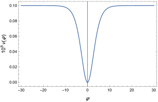
Figure 1 shows the graph of the reduced potential eq. (15) for one of the examples discussed in Ref. AK18 , namely $A=10^{-9}$, $\lambda=1/\sqrt{15}$ and $m=1$, where the T-shape that gives name to these potentials and the two concave plateaus are apparent. Note that the minimum value of the potential is $v_{\mathrm{min}}=v(0)=0$.

Figure 1: Graph of the reduced potential $v(\varphi)=A\left(\tanh^{2}(\lambda\varphi)\right)^{m}$ for $A=10^{-9}$, $\lambda=1/\sqrt{15}$ and $m=1$ (parameters taken from Ref. AK18 ).

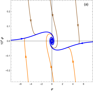
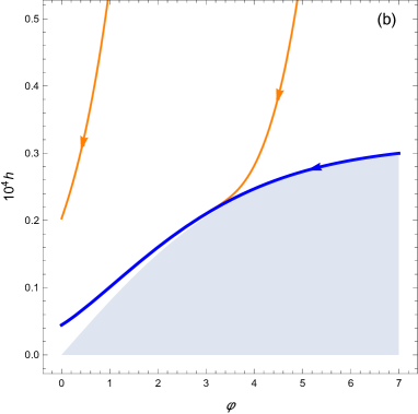
Figure 2(a) shows the phase portrait for this T-model in the $(\varphi,\dot{\varphi})$ plane, and figure 2(b) the corresponding phase portrait in the region $R$ defined by eq. (21) of the Hamilton-Jacobi $(\varphi,h)$ plane, which we now discuss briefly.

Figure 2: (a) Phase portrait in the $(\varphi,\dot{\varphi})$ plane for the potential $v(\varphi)=A\left(\tanh^{2}(\lambda\varphi)\right)^{m}$ for $A=10^{-9}$, $\lambda=1/\sqrt{15}$ and $m=1$. The two blue trajectories are the separatrices. The region $D$ defined in eq. (20) is the fourth quadrant. (b) Corresponding phase portrait in the region $R$ defined by eq. (21) of the Hamilton-Jacobi $(\varphi,h)$ plane. The shaded area is the forbidden region where $h\leq\sqrt{v(\varphi)}$.

In Ref. AM20 we proved that, for a certain class of potentials, if

$$\lim_{\varphi\rightarrow\infty}\frac{v^{\prime}(\varphi)}{2v(\varphi)}=\alpha\quad\mbox{with}\quad 0\leq\alpha<1,$$ (29)

then eq. (24) has a unique solution $h_{s}(\varphi)$ satisfying

$$h_{s}(\varphi)\sim\frac{\sqrt{v(\varphi)}}{\sqrt{1-\alpha^{2}}}\quad\mbox{as}\quad\varphi\rightarrow\infty.$$ (30)

The T-models given by eq. (15) belong to this class of potentials with $\alpha=0$ (incidentally, this $\alpha=0$ is unrelated to the $\alpha$ in eq. (4), and neither of them will appear explicitly in the sequel). Therefore, eq. (24) has a unique solution with asymptotic behavior

$$h_{s}(\varphi)\sim\sqrt{v(\varphi)}\quad\mbox{as}\quad\varphi\rightarrow\infty.$$ (31)

This solution, colored blue in figure (2)(b), is the boundary in the region $R$ of the Hamilton-Jacobi phase space between solutions of eq. (24) defined for all $\varphi>0$ and solutions of eq. (24) that leave $R$ at a certain $\varphi_{*}>0$. The corresponding (full) trajectory in the $(\varphi,\dot{\varphi})$ phase plane, also colored blue in figure (2)(a), spirals in towards the origin and is part of the boundary between regions filled by trajectories that come from large, positive values of $\dot{\varphi}$ (colored brown) and large in magnitude, negative values of $\dot{\varphi}$ (colored orange). The remaining part of the boundary between these trajectories is the symmetric solution. These special solutions are referred to as separatrices, and for wide ranges of initial conditions any solution tends asymptotically to them BE85 ; LID94 . Therefore, separatrices provide accurate approximations to the solutions of the T-model in the SR stage, which will be developed in section 3.

Let us consider now the behavior of the solutions backwards in the cosmic time $t$. Equation (19) shows that the reduced Hubble parameter $h$ is a positive, monotonically decreasing function of $t$. Therefore, the reduced Hubble parameter $h(t)$ increases backwards in time and both $h(t)$ and $\varphi(t)$ may develop singularities. In the KD stage, where

$$\dot{\varphi}^{2}\gg v(\varphi),$$ (32)

we may neglect $v(\varphi)$ in eq. (24) and obtain the approximate equation

$$h^{\prime}(\varphi)\sim\pm h(\varphi),$$ (33)

which yields two families of approximate solutions

$$h(\varphi)\sim\frac{e^{\varphi}}{b}\quad\mbox{as}\quad\varphi\rightarrow\infty,$$ (34)

and

$$h(\varphi)\sim\frac{e^{-\varphi}}{b}\quad\mbox{as}\quad\varphi\rightarrow-\infty,$$ (35)

where $b$ is a strictly positive but otherwise arbitrary parameter. Again, due to the symmetry eq. (28), we can restrict our analysis to solutions with the asymptotic behavior given by eq. (34), for which the integral in the right-hand side of Eq (25) converges as $\varphi\rightarrow\infty$, i.e., these solutions emerge from the KD stage and blow up at a finite time

$$t^{*}=-\int_{\varphi(0)}^{\infty}\frac{d\varphi}{h^{\prime}(\varphi)}.$$ (36)

These singularities, however, lie outside the domain where the KD asymptotic expansions derived in the following section are valid AM22 .

3 Asymptotic expansions

In this section we derive asymptotic expansions for the reduced Hubble parameter $h(\varphi)$ and the number of e-folds $N(\varphi)$ both in the SR and in the KD stages. These computations are most conveniently performed in terms of a new independent variable $y$ defined as

$$y=e^{-2\lambda\varphi},$$ (37)

and the corresponding new functions

$$\hat{h}(y)=h(\varphi),$$ (38)

$$\hat{N}(y)=N(\varphi).$$ (39)

Substituting eqs. (37) and (38) into eq. (24) with the potential given by eq. (15), we find the following equation for $\hat{h}(y)$,

$$4\lambda^{2}y^{2}\hat{h}^{\prime}(y)^{2}-\hat{h}(y)^{2}+A\left(\frac{1-y}{1+y}\right)^{2m}=0,$$ (40)

and substituting into eq. (27), the following equation for $\hat{N}(y)$,

$$\hat{N}^{\prime}(y)=\frac{1}{12\lambda^{2}y^{2}}\frac{\hat{h}(y)}{\hat{h}^{\prime}(y)}.$$ (41)

3.1 The Hubble parameter in the SR stage

As we discussed in section 2.3, the separatrix is an accurate approximation to the solutions in the SR stage, and since the separatrix is uniquely identified by the asymptotic behavior given in eq. (31), we look for an asymptotic solution of eq. (40) in the form of the leading asymptotic prefactor times a power series in $y$,

$$\hat{h}_{\text{SR}}(y)=\sqrt{A}\left(\frac{1-y}{1+y}\right)^{m}\left(1+8m^{2}\lambda^{2}\sum_{n=2}^{\infty}(-1)^{n}c_{n}y^{n}\right).$$ (42)

By substituting this ansatz into eq. (40) we find that $c_{2}=1$ and that the unknown coefficients $c_{n}$ (which depend on $\lambda$ and $m$) can be computed from the recurrence relation

$$c_{n} = 8m\lambda^{2}(n-1)c_{n-1}+2(1+8m^{2}\lambda^{2})c_{n-2}-8m\lambda^{2}(n-3)c_{n-3}-c_{n-4}$$ (43)

$${}-4m^{2}\lambda^{2}\Big{(}\sum_{j=2}^{n-6}c_{j}c_{n-4-j}-2\sum_{j=2}^{n-4}c_{j}c_{n-2-j}+\sum_{j=2}^{n-2}c_{j}c_{n-j}\Big{)}$$

$${}+16m^{2}\lambda^{4}\sum_{j=1}^{n-3}[(j+1)c_{j+1}+2mc_{j}-(j-1)c_{j-1}]$$

$$\qquad\qquad\qquad\times[(n-j-1)c_{n-j-1}+2mc_{n-j-2}-(n-j-3)c_{n-j-3}],$$

where we have set $c_{n}=0$ for $n<2$. The resulting even and odd coefficients can be written as,

$$c_{2j}=\sum_{k=0}^{j-1}(m\lambda)^{2k}p_{2j}^{(k)}(\lambda^{2}),$$ (44)

$$c_{2j+1}=m\lambda^{2}\sum_{k=0}^{j-1}(m\lambda)^{2k}p_{2j+1}^{(k)}(\lambda^{2}),$$ (45)

respectively, where the $p_{n}^{(k)}(\lambda^{2})$ are polynomials of degree $k$ in $\lambda^{2}$ which we list in Table 1 up to $n=9$.

$n$	$k$	$p_{n}^{(k)}(\lambda^{2})$
$2$	$0$	$1$
$3$	$0$	$16$
$4$	$0$	$2$
	$1$	$12+448\lambda^{2}$
$5$	$0$	$80$
	$1$	$640+17408\lambda^{2}$
$6$	$0$	$3$
	$1$	$48+4096\lambda^{2}$
	$2$	$160+36352\lambda^{2}+847872\lambda^{4}$
$7$	$0$	$224$
	$1$	$4480+248832\lambda^{2}$
	$2$	$17920+2326528\lambda^{2}+49020928\lambda^{4}$
$8$	$0$	$4$
	$1$	$120+18304\lambda^{2}$
	$2$	$960+392192\lambda^{2}+17276928\lambda^{4}$
	$3$	$2240+1714176\lambda^{2}+166674432\lambda^{4}+3255828480\lambda^{6}$
$9$	$0$	$480$
	$1$	$17280+1612800\lambda^{2}$
	$2$	$161280+35618816\lambda^{2}+1340866560\lambda^{4}$
	$3$	$430080+163872768\lambda^{2}+13211009024\lambda^{4}+243139608576\lambda^{6}$

Table 1: Polynomials $p_{n}^{(k)}(\lambda^{2})$ that give the coefficients $c_{n}$ (up to $n=9$) in the formal expansion of the separatrix $\hat{h}_{\text{SR}}(y)$ as functions of the parameters $m$ and $\lambda$ for the T-models with reduced potentials $v(\varphi)=A(\tanh^{2}(\lambda\varphi))^{m}$.

3.2 The number of e-folds in the SR stage

The corresponding asymptotic expansion for the number of e-folds in the SR stage follows immediately from eq. (41),

$$\hat{N}_{\text{SR}}(y)-\hat{N}_{\text{SR},0}=\frac{1}{12\lambda^{2}}\int\frac{\hat{h}_{\text{SR}}(y)}{\hat{h}_{\text{SR}}^{\prime}(y)}\frac{dy}{y^{2}}.$$ (46)

After term by term integration and separation of the leading factors we get an asymptotic expansion which we write in the form

$$\hat{N}_{\text{SR}}(y)-\hat{N}_{\text{SR},0}=\frac{1}{24m\lambda^{2}}\left(y+\frac{1}{y}\right)-\frac{1}{3}\log y+\sum_{n=1}^{\infty}(-1)^{n+1}\gamma_{n}y^{n}.$$ (47)

Note that there are two terms in $y$ in this expansion: one in the term between parentheses and one in the formal series. The reason for this choice is that (aside from the dependence of the integration constant) the term in parentheses leads directly to the standard SR approximation eq. (9). The coefficients $\gamma_{n}$ can be readily calculated from the $c_{2},\ldots,c_{n+2}$ during the integration. For example,

$$\gamma_{1} = \frac{16}{3}m\lambda^{2},$$ (48)

$$\gamma_{2} = \frac{1}{3}+\frac{8}{3}m^{2}\lambda^{2}+96m^{2}\lambda^{4},$$ (49)

$$\gamma_{3} = \frac{112}{9}m\lambda^{2}+\frac{1024}{9}m^{3}\lambda^{3}+\frac{28672}{9}m^{3}\lambda^{6},$$ (50)

but a more efficient method to compute these coefficients is to substitute eqs. (42) and (47) into eq. (41), obtaining directly the relation between the $\gamma_{n}$ and the $c_{n}$. Thus, we reproduce eqs. (48)–(50) and find that for $n\geq 4$,

$$\gamma_{n} = \frac{1}{6n}\Big{[}(n+2)c_{n+2}-nc_{n}+2mc_{n-1}-8m\lambda^{2}\left((n+1)c_{n+1}+2mc_{n}-(n-1)c_{n-1}\right)$$ (51)

$${}-(1+24m\lambda^{2}\gamma_{1})(nc_{n}+2mc_{n-1}-(n-2)c_{n-2})-48m\lambda^{2}(n-1)\gamma_{n-1}$$

$${}-24m\lambda^{2}\sum_{j=3}^{n-1}\left((n+2-j)c_{n+2-j}+2mc_{n+1-j}-(n-j)c_{n-j}\right)(j-1)\gamma_{j-1}\Big{]}.$$

3.3 The Hubble parameter in the KD stage

Similarly, to find an asymptotic expansion for the reduced Hubble parameter in the KD stage we have to look for a formal solution of eq. (40) with leading asymptotic behavior given by eq. (34). However, as we mentioned in the Introduction, and because of this leading asymptotic behavior, this formal solution has to be of the form,

$$\hat{h}_{\text{KD}}(y,b)=\frac{1}{by^{\frac{1}{2\lambda}}}+\sum_{n=1}^{\infty}A^{n}b^{2n-1}\zeta_{n}(y)y^{\frac{2n-1}{2\lambda}},$$ (52)

where $\zeta_{n}(y)$ are in turn formal power series in $y$,

$$\zeta_{n}(y)=\sum_{p=0}^{\infty}(-1)^{p}\zeta_{n,p}y^{p}.$$ (53)

For the computation of the coefficients $\zeta_{n,p}$ we assume temporarily that $\lambda$ is not a rational number, which makes integer powers of $y$ and of $y^{\frac{1}{2\lambda}}$ linearly independent, and thus allows independent identification of the corresponding coefficients. A limiting argument shows that our results are still valid for rational values of $\lambda$, and a somewhat lengthy computation shows that the coefficients are determined recursively by

$$\zeta_{1,0} = \frac{1}{4},$$ (54)

$$\zeta_{1,p} = \frac{1}{4(1+p\lambda)}\sum_{j=0}^{p}2^{j}\binom{2m}{j}\binom{p-1}{j-1},\quad(p=1,2,\ldots),$$ (55)

$$\zeta_{n+1,p}=\frac{1}{n+1+p\lambda}\sum_{j=1}^{n}\sum_{r=0}^{p}\left[\left(j+r\lambda-\frac{1}{2}\right)\left(n-j+(p-r)\lambda+\frac{1}{2}\right)-\frac{1}{4}\right]\zeta_{j,r}\zeta_{n+1-j,p-r}.$$ (56)

Since eq. (56) for $p=0$ takes the form

$$\zeta_{n+1,0}=\frac{1}{n+1}\sum_{j=1}^{n}\left[\left(j-\frac{1}{2}\right)\left(n-j+\frac{1}{2}\right)-\frac{1}{4}\right]\zeta_{j,0}\zeta_{n+1-j,0},$$ (57)

by setting $n=1$ we find that $\zeta_{2,0}=0$, and by induction that $\zeta_{n,0}=0$ for all $n\geq 2$. For example, the first three coefficients are,

$$\zeta_{1}(y)=\frac{1}{4}-\frac{m}{\lambda+1}y+\frac{2m^{2}}{2\lambda+1}y^{2}+\cdots,$$ (58)

$$\zeta_{2}(y)=-\frac{\lambda m}{4\left(\lambda+1\right)\left(\lambda+2\right)}y+\frac{\lambda(3\lambda+2)m^{2}}{2(\lambda+1)^{2}(2\lambda+1)}y^{2}+\cdots,$$ (59)

$$\zeta_{3}(y)=-\frac{\lambda m}{16(\lambda+2)(\lambda+3)}y+\frac{\lambda\left(7\lambda^{2}+16\lambda+6\right)m^{2}}{8(\lambda+1)^{2}(\lambda+2)(2\lambda+3)}y^{2}+\cdots.$$ (60)

3.4 The number of e-folds in the KD stage

Similarly, asymptotic solutions for the number of e-folds in the KD stage have the form,

$$\hat{N}_{\text{KD}}(y,b)-\hat{N}_{\text{KD},0}(b)=-\frac{\log y}{6\lambda}-\sum_{n=1}^{\infty}A^{n}b^{2n}\xi_{n}(y)y^{\frac{n}{\lambda}},$$ (61)

where

$$\xi_{n}(y)=\sum_{p=0}^{\infty}(-1)^{p}\xi_{n,p}y^{p},$$ (62)

and using eq. (41) we find that the coefficients $\xi_{n,p}$ can be computed recursively from

$$\xi_{1,p}=\frac{1}{3}\zeta_{1,p},$$ (63)

and for $n\geq 2$

$$\xi_{n,p}=\frac{1}{3}\zeta_{n,p}+\frac{1}{n+p\lambda}\sum_{j=1}^{n-1}\sum_{r=0}^{p}\left[(j+r\lambda)(2(n-j)+2(p-r)\lambda-1)\right]\xi_{j,r}\zeta_{n-j,p-r}.$$ (64)

The first three coefficients are,

$$\xi_{1}(y)=\frac{1}{12}-\frac{m}{3(\lambda+1)}y+\frac{2m^{2}}{3(2\lambda+1)}y^{2}+\cdots,$$ (65)

$$\xi_{2}(y)=\frac{1}{96}-\frac{(2\lambda+1)m}{6(\lambda+1)(\lambda+2)}y+\frac{\left(5\lambda^{2}+5\lambda+1\right)m^{2}}{3(\lambda+1)^{2}(2\lambda+1)}y^{2}+\cdots,$$ (66)

$$\xi_{3}(y)=\frac{1}{576}-\frac{\left(9\lambda^{2}+19\lambda+6\right)m}{48(\lambda+1)(\lambda+2)(\lambda+3)}y+\frac{\left(90\lambda^{4}+313\lambda^{3}+338\lambda^{2}+141\lambda+18\right)m^{2}}{24(\lambda+1)^{2}(\lambda+2)(2\lambda+1)(2\lambda+3)}y^{2}+\cdots.$$ (67)

4 Matching of the SR and KD asymptotic expansions

In the previous section we have found asymptotic solutions

$$h_{\text{SR}}(\varphi)=\hat{h}_{\text{SR}}(e^{-2\lambda\varphi}),\quad N_{\text{SR}}(\varphi)=\hat{N}_{\text{SR}}(e^{-2\lambda\varphi}),$$ (68)

and

$$h_{\text{KD}}(\varphi,b)=\hat{h}_{\text{KD}}(e^{-2\lambda\varphi},b),\quad N_{\text{KD}}(\varphi,b)=\hat{N}_{\text{KD}}(e^{-2\lambda\varphi},b),$$ (69)

of eqs. (24) and (27) valid, in principle, in the SR and KD stages respectively. In this section we discuss how to match these asymptotic solutions to cover the whole inflation region, thereby allowing us to obtain approximate values of relevant magnitudes as functions of the parameter $b$ in eq. (34), or equivalently, as functions of the initial conditions, which in turn will allow us to find initial conditions that correspond to a previously fixed amount of inflation. In particular, we will see that the $h_{\text{KD}}(\varphi,b)$ asymptotic expansion, when appropriately summed, extends its domain of validity beyond the region where eq. (32) is satisfied and enters the so called “fast roll” stage.

From the Hamilton-Jacobi eqs. (23) and (24) it follows that

$$\ddot{a}=\frac{a}{3}\left(v(\varphi)-\frac{2}{3}h(\varphi)^{2}\right),$$ (70)

and therefore the inflation region $\ddot{a}>0$ corresponds to the interval of $\varphi$ that satisfies

$$\sqrt{v(\varphi)}<h(\varphi)<\sqrt{\frac{3}{2}v(\varphi)}$$ (71)

(the lower bound is just eq. (21)). This interval (traveled from right to left in our plots) begins at a value $\varphi_{\text{in}}(b)$ in the KD stage at which

$$h_{\text{KD}}(\varphi_{\text{in}}(b),b)=\sqrt{\frac{3}{2}v(\varphi_{\text{in}}(b))}.$$ (72)

Note that the dependency of $\varphi_{\text{in}}$ on $b$ encodes the initial condition. Similarly, we assume that the interval ends at a value $\varphi_{\text{end}}$ in the SR stage, which, since we have approximated all the solutions in the SR stage by the separatrix, will be independent of $b$, and at which

$$h_{\text{SR}}(\varphi_{\text{end}})=\sqrt{\frac{3}{2}v(\varphi_{\text{end}})}.$$ (73)

To determine an intermediate value $\varphi_{*}(b)$ such that $h(\varphi)$ is well approximated by $h_{\text{SR}}(\varphi)$ on $[\varphi_{\text{end}},\varphi_{*}(b)]$, by $h_{\text{KD}}(\varphi,b)$ on $[\varphi_{*}(b),\varphi_{\text{in}}(b)]$, and by both on a neighborhood of $\varphi_{*}(b)$, we select $\varphi_{*}(b)$ as the first local minimum of $(h_{\text{KD}}(\varphi,b)-h_{\text{SR}}(\varphi))^{2}$, i.e., the local minimum closest to $\varphi_{\text{in}}(b)$. Next, to determine the integration constants $\hat{N}_{\text{SR},0}$ and $\hat{N}_{\text{KD},0}(b)$ in the asymptotic expansions for $N$, we first fix the origin from which we count the amount of inflation by $N_{\text{SR}}(\varphi_{\text{end}})=0$, i.e.,

$$\hat{N}_{\text{SR}}(e^{-2\lambda\varphi_{\text{end}}})=0,$$ (74)

and then determine $\hat{N}_{\text{KD},0}(b)$ by continuity at $\varphi_{*}(b)$, i.e., by

$$\hat{N}_{\text{SR}}(e^{-2\lambda\varphi_{*}(b)})=\hat{N}_{\text{KD}}(e^{-2\lambda\varphi_{*}(b)},b).$$ (75)

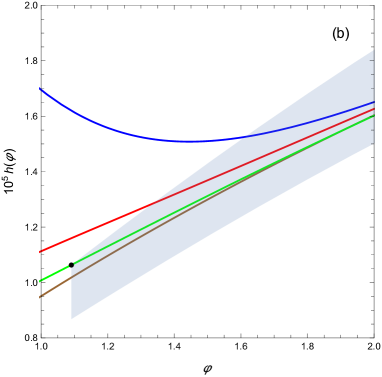
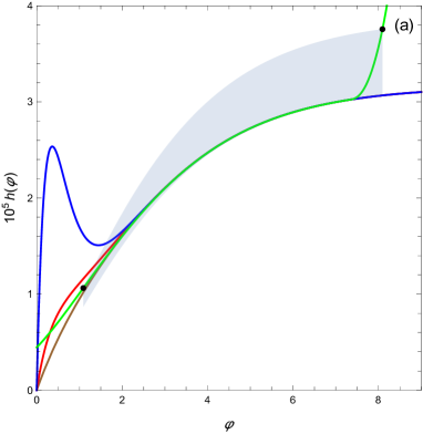
However, implicit in the former discussion of the matching procedure is the fact that we are dealing with asymptotic expansions that need to be either appropriately truncated or summed, and in particular whether there exists a neighborhood of $\varphi_{*}(b)$ on which the truncated or summed expansions are both accurate. We consider first the SR asymptotic expansion. The green curve in figure 3 is the result of a numerical integration for the T-model with $A=10^{-9}$, $\lambda=1/\sqrt{15}$ and $m=1$ with initial condition $h(\varphi_{0})=2\times 10^{-4}$ at $\varphi_{0}=10$ (outside the range shown in the figure). The shaded region is the inflation region as defined in eq. (71), and the brown, red, and blue curves correspond to the partial sums of the formal series in eq. (42) to $n_{\text{SR}}=2$, $4$ and $6$ terms, respectively. Figure 3(a) shows that (in part because of the leading behavior as $\varphi\to\infty$ built in eq. (42)) all these partial sums give excellent approximations at large $\varphi$, but the magnification in figure 3(b) shows that partial sums are clearly insufficient to approximate accurately the reduced Hubble parameter in a neighborhood of $\varphi_{\text{end}}\approx 1.091$, and, as is typical of partial sums of asymptotic expansions, get progressively worse, despite the fact that the prefactor in eq. (42) enforces $h(0)=0$. To circumvent this problem and in light of the alternating sign apparent in the first terms of eq. (42) (for which we do not have a proof), we use Padé $[n_{\text{SR}}/n_{\text{SR}}+1]$ approximants to sum the formal series. At the scale of figure 3, already the $[2/3]$ Padé approximant (not shown) would be superimposed to the numerical integration (green curve). The errors of the Padé approximants at $\varphi_{\text{end}}\approx 1.091$ (black dot) decrease from $2.14\%$ for $n_{\text{SR}}=2$, to $0.49\%$ for $n_{\text{SR}}=4$, and stabilize at $0.023\%$ for $n_{\text{SR}}=12$ and higher approximants, which accounts for the difference between the numerical $h(\varphi_{\text{end}})$ of our initial value problem and the value of the separatix at that point to which the asymptotic series $h_{\text{SR}}(\varphi_{\text{end}})$ is being summed by the Padé approximants.

Figure 3: Numerical integration (green curve) and partial sums of $h_{\text{SR}}(\varphi)$ to $n_{\text{SR}}=2$, $4$, and $6$ terms (brown, red and blue curves, respectively) for a T-model with $A=10^{-9}$, $\lambda=1/\sqrt{15}$ and $m=1$ with initial condition $h(\varphi_{0})=2\times 10^{-4}$ at $\varphi_{0}=10$ (outside the range of the figure): (a) Inflation region as given by eq. (71); (b) Magnification around $\varphi_{\text{end}}\approx 1.091$.

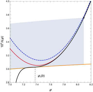
We consider next the KD asymptotic expansion. Figure 4 shows a neighborhood of $\varphi_{\text{in}}\approx 8.092$, where the green curve (barely visible) is the same curve as in figure 3 and the orange curve is the Padé-summed SR asymptotic expansion with $n_{\text{SR}}=12$ (as we explained earlier, Padé summation of $h_{\text{SR}}(\varphi)$ is unnecessary for these values of $\varphi$ but essential in the neighborhood of $\varphi_{\text{end}}$), and the red and black curves are, respectively, the $n_{\text{KD}}=2$ and $n_{\text{KD}}=16$ summations of the double series for $h_{\text{KD}}(\varphi,b)$ with $b=1.10817\times 10^{8}$, where, for consistency (and taking into account typical values of $\lambda$), the $n_{\text{KD}}$ summation is defined by

$$\hat{h}_{\text{KD}}^{[n_{\text{KD}}]}(y,b)=\frac{1}{by^{\frac{1}{2\lambda}}}+\sum_{n=1}^{\lfloor 2\lambda n_{\text{KD}}\rfloor}A^{n}b^{2n-1}\zeta_{k_{n},k_{n}+1}(y)y^{\frac{2n-1}{2\lambda}},$$ (76)

where $\lfloor x\rfloor$ denotes the greatest integer less than or equal to $x$,

$$k_{n}=\lfloor n_{\text{KD}}-n/(2\lambda)\rfloor,$$ (77)

and $\zeta_{k_{n},k_{n}+1}(y)$ denotes the $[k_{n}/k_{n}+1]$ Padé approximant to $\zeta_{n}(y)$. The value of $b$ has been chosen so that the summed $h_{\text{KD}}(\varphi_{0},b)=h(\varphi_{0})$, and the figure shows that the $n_{\text{KD}}=2$ approximation (red curve) does not yet match the SR approximation (orange curve), but the $n_{\text{KD}}=16$ does match it, and allows us to solve for $\varphi_{*}(b)$ as the first local minimum of $(h_{\text{KD}}(\varphi,b)-h_{\text{SR}}(\varphi))^{2}$, which turns out to be $\varphi_{*}(b)\approx 7.372$. Finally, the blue, dashed line represents a noteworthy first order approximation derived by Chowdhury, Martin, Ringeval and Vennin in Ref. CM19 , which in our notation reads,

$$h(\varphi)\approx\frac{1}{2}(c_{+}e^{\varphi-\varphi_{0}}+c_{-}e^{-(\varphi-\varphi_{0})}),$$ (78)

where

$$c_{\pm}=h(\varphi_{0})\pm\sqrt{h(\varphi_{0})^{2}-v(\varphi_{0})}.$$ (79)

Figure 4 shows that this approximation is remarkably accurate for a first-order approximation, but is not accurate enough to be matched with the SR approximation.

Figure 4: Numerical integration of $h(\varphi)$ (green curve), summation of $h_{\text{SR}}(\varphi)$ for $n_{\text{SR}}=12$, (orange curve), summations of $h_{\text{KD}}(\varphi,b)$ for $n_{\text{KD}}=2$ (red curve) and $n_{\text{KD}}=16$ (black curve), and first-order approximation from Ref. CM19 (blue, dashed curve). The vertical line at $\varphi_{*}(b)\approx 7.372$ marks the matching point. The numerical (green) curve is barely visible because of the accurate approximations provided by the SR (orange) curve up to $\varphi_{*}(b)$ and the KD (black) curve from $\varphi_{*}(b)$ onwards.

As we discussed above, the constant $\hat{N}_{\text{SR},0}$ is a choice of origin, while matching the asymptotic expansions for the reduced Hubble parameter determines the constant $\hat{N}_{\text{KD},0}$ in eq. (61) via eq. (75). In practice we use an expression analogous to eq. (76),

$$\hat{N}_{\text{KD}}^{[n_{\text{KD}}]}(y,b)-\hat{N}_{\text{KD},0}(b)=-\frac{\log y}{6\lambda}-\sum_{n=1}^{\lfloor 2\lambda n_{\text{KD}}\rfloor}A^{n}b^{2n}\xi_{k_{n},k_{n}+1}(y)y^{\frac{n}{\lambda}},$$ (80)

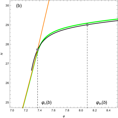
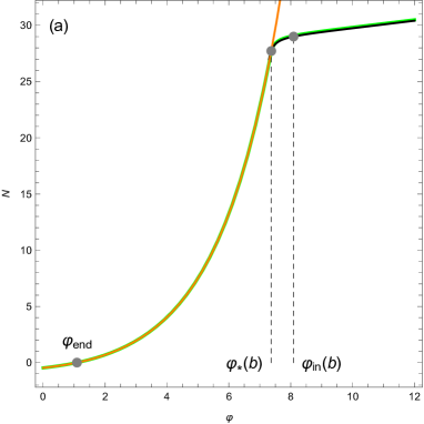
but at the risk of being repetitive we stress that the procedure to determine $\hat{N}_{\text{KD},0}$ is not a matching—the expansions that are matched are the expansions for the reduced Hubble parameter. To illustrate this point, in figure 5 we show the result of the numerical integration for $N(\varphi)$ (the green curve corresponding to the green curves is figures 3 and 4), the $n_{\text{SR}}=16$ summation of $N_{\text{SR}}(\varphi)$ (the orange curve), and the $n_{\text{KD}}=16$ summation of $N_{\text{KD}}(\varphi,b)$ (the black curve). The magnification in figure 5(b) shows how the matching at $\varphi_{*}(b)$ shown in figure 4 induces a crossing between the summations of the expansions for the scale factor that mimics the inflection point of the numerical integration. Because of eq. (27), the numerical integration for $N(\varphi)$ is more sensitive to the initial conditions than the numerical integration for $h(\varphi)$, but the Padé-summed asymptotic expansion for $N_{\text{KD}}(\varphi,b)$ gives a remarkably accuracy up to the crossing point.

Figure 5: Numerical integration for $N(\varphi)$ (green curve), summation of $N_{\text{SR}}(\varphi,b)$ for $n_{\text{SR}}=16$, (orange curve), and summation of $N_{\text{KD}}(\varphi,b)$ for $n_{\text{KD}}=16$ (black curve): (a) on the inflation interval $[\varphi_{\text{end}},\varphi_{\text{in}}(b)]$; (b) magnification of a neighborhood of $\varphi_{*}(b)$ showing how the crossing between the summations mimic the inflection point of the numerical integration.

5 Applications

The approximations to the reduced Hubble parameter $h(\varphi)$ and to the number of e-folds $N(\varphi)$ on the whole inflation interval $[\varphi_{\text{end}},\varphi_{\text{in}}(b)]$ that the matching procedure discussed in the previous section produces allows us to derive ensuing approximations to several relevant magnitudes as functions of the parameter $b$ (or, equivalently, of the initial conditions), e.g., the values of the inflaton for which a solution enters and exits the inflation region or the total amount of inflation, or, conversely, to find the initial conditions for a solution to correspond to a previously fixed total amount of inflation.

Example	$A$	$m$	$\lambda$
I	$10^{-9}$	$1$	$1/\sqrt{15}$
II	$10^{-9}$	$7/8$	$1/3$

Table 2: Parameters for the T-models used in section 5. The values of $m$ and $\lambda$ for Example I and II are taken from Refs. AK18 , and CA15 , respectively. The values of $A$ are derived from typical values of $\Lambda$.

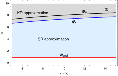
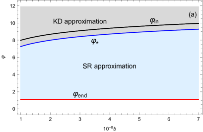
We illustrate these applications with two examples whose parameters, summarized in Table 2, are chosen according to the following considerations. Our first example has $m=1$ and $\alpha=5/3$ (or, using eq. (16), $\lambda=1/\sqrt{15}$) AK18 . The corresponding values of $\Lambda$ found in the literature range from $\Lambda=\alpha 10^{-10}\mathrm{M}_{\mathrm{Pl}}^{2}$ CA15 ; AK18 to $\Lambda=10^{-8}\mathrm{M}_{\mathrm{Pl}}^{2}$ SD20 . Using again eq. (16), we have taken as a typical value $A=10^{-9}$. Incidentally, this is the potential shown in figure 1 with the corresponding phase portrait shown in figure 2. Our second example, taken from Ref. CA15 , has the noninteger value of $m=7/8$, $\alpha=1$ (i.e., $\lambda=1/3$), and again the typical value $A=10^{-9}$. Before proceeding to the applications proper, in Fig 6 we summarize the results of the matching for both examples as a function of the parameter $b$ for $n_{\text{SR}}=n_{\text{KD}}=16$. The constants $\hat{N}_{\text{SR},0}$ (determined via eq. (74) for Examples I and II are $-1.69$ and $-1.31$, respectively. Figures 6(a) and (b) show the values of $\varphi_{\text{end}}$ (constant), $\varphi_{*}(b)$ and $\varphi_{\text{in}}(b)$ for Example I and Example II respectively. We recall that the Padé summation provides an SR approximation to the separatrix accurate on $[\varphi_{\text{end}},\infty)$, and a KD approximation for a particular, $b$-dependent solution valid on $[\varphi_{*}(b),\infty)$. These intervals are illustrated by the shaded regions in the figure. The values for $\hat{N}_{\text{KD},0}(b)$ defined in eq. (61) and computed according to eq. (75) for Examples I and II are shown in figures 6(c) and (d) respectively.

Figure 6: Results of the matching of the $n_{\text{SR}}=16$ and $n_{\text{KD}}=16$ approximants for the T-models of Table 2 as functions of the parameter $b$: (a), (b) $\varphi_{\text{end}}$ (constant, red line), $\varphi_{*}(b)$ (blue line) and $\varphi_{\text{in}}(b)$ (black line) for Example I and Example II respectively; (c), (d) $\hat{N}_{\text{KD},0}(b)$ for Example I and Example II respectively.

5.1 The total amount of inflation as a function of the initial condition

The total amount of inflation or number of e-folds during the inflation period is

$$N_{T}=\log\frac{a(t_{\text{end}})}{a(t_{\text{in}})}=N(\varphi_{\text{in}})-N(\varphi_{\text{end}})=N(\varphi_{\text{in}}),$$ (81)

which we approximate by

$$N_{T}\approx\hat{N}_{\text{KD}}^{[n_{\text{KD}}]}(y_{\text{end}},b),$$ (82)

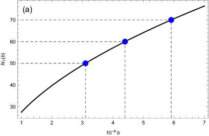
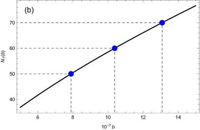
and should be close to $N_{T}\approx 60$ BA09 ; BA12 ; DO03 ; MA18 . Figure 7 shows the result of a calculation with $n_{\text{SR}}=16$ and $n_{\text{KD}}=16$ for the two examples in Table 2, and Table 3 shows a comparison of the results obtained from the asymptotic expansions for $N_{T}(b)=50$, $60$ and $70$ (the marked points on figure 7) with the results of a numerical integration. More concretely, for each value of $N_{T}$ we find the corresponding value of $b$ in figure 7 and perform a numerical integration of eqs. (24) and (27) with initial conditions at $\varphi_{0}=10$ given by $h(\varphi_{0})=h_{\text{KD}}(\varphi_{0},b)$ and $N(\varphi_{0})=N_{\text{KD}}(\varphi_{0},b)$. In all the cases we have tested, the errors are below $0.5\%$, i.e., well below one e-fold. Note also that the number of e-folds outside the SR stage is only about 1.2.

Figure 7: Approximate total amount of inflation $N_{T}(b)$ as a function of the parameter $b$ for $n_{\text{SR}}=16$ and $n_{\text{KD}}=16$. The dots mark $N_{T}=50$, $60$ and $70$: (a) Example I in Table 2; (b) Example II in Table 2.

	Example I			Example II
$N_{T}(b)$	$b$	$N_{T}^{\text{(num)}}(b)$	$N_{\text{SR}}(\varphi_{*}(b))$	$b$	$N_{T}^{\text{(num)}}(b)$	$N_{\text{SR}}(\varphi_{*}(b))$
50	$3.10\times 10^{8}$	50.03	48.98	$7.89\times 10^{7}$	50.03	48.83
60	$4.40\times 10^{8}$	60.00	58.92	$1.04\times 10^{8}$	60.06	58.84
70	$5.91\times 10^{8}$	70.00	68.93	$1.31\times 10^{8}$	70.09	68.85

Table 3: Comparison between the total amount of inflation $N_{T}(b)$ with $n_{\text{SR}}=16$ and $n_{\text{KD}}=16$ and the result of a numerical integration from the corresponding initial condition $b$. $N_{\text{SR}}(b)$ denotes the number of e-folds in the SR stage.

As we mentioned in the Introduction, eq. (9), which written in terms of reduced variables reads

$$N^{\text{(SR)}}(\varphi)=\frac{1}{12m\lambda^{2}}\left(\cosh(2\lambda\varphi)-\sqrt{1+12m^{2}\lambda^{2}}\right),$$ (83)

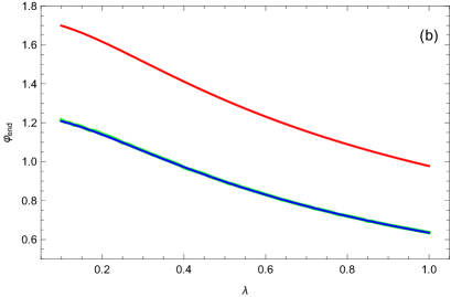
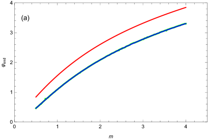
cannot directly be used to compute the total amount of inflation, but it gives accurate results for the spectral indexes as functions of the number of e-folds despite omitting the kinetic term altogether. To understand this fact, in Figure 8 we plot the values of $\varphi_{\text{end}}$ given by the standard SR approximation eq. (8), by eq. (73) with $n_{\text{SR}}=16$, and by a numerical integration first, in panel (a), as a function of the parameter $m$ for a fixed value of $\lambda$, and then, in panel (b), as a function of the parameter $\lambda$ for a fixed value of $m$. The key observation is that for a wide range of parameter models the standard SR approximation consistently overestimates the value of $\varphi_{\text{end}}$, thus compensating for missing the KD stage of inflation.

Figure 8: (a) End of inflation $\varphi_{\text{end}}$ as a function of the parameter $m$ for T-models with $A=10^{-9}$, $\lambda=1/\sqrt{15}$ and initial condition $h(\varphi_{0})=4\times 10^{-4}$ at $\varphi_{0}=10$. The red curve is the result given by eq. (8), the blue curve is the result given by eq. (73) with $n_{\text{SR}}=16$, and the green curve is the result of a numerical integration. (b) End of inflation $\varphi_{\text{end}}$ as a function of the parameter $\lambda$ for T-models with $A=10^{-9}$, $m=1$ and initial condition $h(\varphi_{0})=3\times 10^{-4}$ at $\varphi_{0}=10$. The red curve is the result given by eq. (8), the blue curve is the result given by eq. (73) with $n_{\text{SR}}=16$, and the green curve is the result of a numerical integration.

5.2 Second order corrections to the spectral indexes in the SR approximation

The spectral indexes $n_{s}$ and $r$ for T-models in the first-order SR approximation are given by

$$n_{s}=1-\frac{2}{N},$$ (84)

and

$$r=\frac{4}{3\lambda^{2}N^{2}},$$ (85)

although the latter equation is often written in terms of $\alpha$ instead of $\lambda$ KL13 ; KL13b ; KALL15 ; GA15 ; CA15 ; AK18 ; AC21 . Note in particular that the first-order approximation to $n_{s}$ is independent of the parameters of the model. There have been some attempts to find higher-order corrections to these formulas KA13 ; OO16 ; GE21 , but lacking the necessary terms in the expansions they seem not to be completely consistent. In this section, and taking advantage of our former results, we compute the spectral indexes $n_{s}(N)$ and $r(N)$ to second order in the SR approximation or, more precisely, to order $1/N^{2}$ and $1/N^{3}$ respectively. To this aim, we consider the $O(\epsilon_{i}^{3})$ expressions LE02 ,

$$n_{s}=1-2\epsilon_{1}-\epsilon_{2}-2\epsilon_{1}^{2}-(2C+3)\epsilon_{1}\epsilon_{2}-C\epsilon_{2}\epsilon_{3},$$ (86)

and

$$r=16\epsilon_{1}\left[1+C\epsilon_{2}+\left(C-\frac{\pi^{2}}{2}+5\right)\epsilon_{1}\epsilon_{2}+\left(\frac{C^{2}}{2}-\frac{\pi^{2}}{8}+1\right)\epsilon_{1}^{2}+\left(\frac{C^{2}}{2}-\frac{\pi^{2}}{24}\right)\epsilon_{2}\epsilon_{3}\right],$$ (87)

where $C$ can be written in terms of the Euler-Mascheroni constant $\gamma$,

$$C=\gamma+\log 2-2,$$ (88)

and the slow-roll parameters $\epsilon_{1}$, $\epsilon_{2}$, and $\epsilon_{3}$ can be written as functions of $N^{\prime}(\varphi)$ (cf. eq. (27)) and its derivatives,

$$\epsilon_{1}(\varphi)=\frac{1}{3}\frac{1}{N^{\prime}(\varphi)^{2}},$$ (89)

$$\epsilon_{2}(\varphi)=-2\frac{d}{d\varphi}\frac{1}{N^{\prime}(\varphi)},$$ (90)

$$\epsilon_{2}(\varphi)\epsilon_{3}(\varphi)=\frac{2}{N^{\prime}(\varphi)}\frac{d^{2}}{d\varphi^{2}}\frac{1}{N^{\prime}(\varphi)}.$$ (91)

We will see later that although all the terms in eq. (86) are required, only the first two terms in eq. (87) need to be considered.

Since all our expansions in this section pertain to the SR stage, hereafter we drop the subindex “SR” but keep the circumflex accent to denote magnitudes in the variable $y$. By substituting eq. (39) and the second order approximation

$$\hat{N}(y)=\hat{N}_{0}+\frac{1}{24m\lambda^{2}}\left(1+\frac{1}{y}\right)-\frac{1}{3}\log y-\frac{16}{3}m\lambda^{2}y+O(y^{2}),$$ (92)

into eqs. (89)–(91) we find that,

$$\hat{\epsilon}_{1}(y)=\frac{48m^{2}\lambda^{2}y^{2}}{(1-y^{2})^{2}}(1-16m\lambda^{2}y+O(y^{2})),$$ (93)

$$\hat{\epsilon}_{2}(y)=\frac{48m\lambda^{2}y(1+y^{2})}{(1-y^{2})^{2}}(1-16m\lambda^{2}y+O(y^{2})),$$ (94)

$$\hat{\epsilon}_{2}(y)\hat{\epsilon}_{3}(y)=\frac{1152m^{2}\lambda^{4}y^{2}(1+6y^{2}+y^{4})}{(1-y^{2})^{4}}(1+O(y)).$$ (95)

Note that the second order approximation (92) differs from the standard SR approximation (9) in both the logarithmic term and the first term in the series in eq. (47).

Then, we need to find the value of $y_{\text{end}}$ corresponding to the end of the inflationary stage to second order in the SR approximation, i.e., to solve

$$\hat{\epsilon}_{1}(y_{\text{end}})=1$$ (96)

to second order. The first order approximation is the suitable solution of the simple biquadratic equation

$$\frac{48m^{2}\lambda^{2}y^{2}}{(1-y^{2})^{2}}=1,$$ (97)

namely

$$y_{\text{end},1}=\sqrt{1+12m^{2}\lambda^{2}}-2\sqrt{3}m\lambda,$$ (98)

and the second order correction is obtained by substituting $y=y_{\text{end},1}+y_{\text{end},2}$ into eq. (96) and expanding to first order in $y_{\text{end},2}$ using eq. (93). The full result turns out to be,

$$y_{\text{end}}=(\sqrt{1+12m^{2}\lambda^{2}}-2\sqrt{3}m\lambda)\left(1+\frac{48m^{2}\lambda^{3}}{\sqrt{1+12m^{2}\lambda^{2}}(6m\lambda+\sqrt{3}\sqrt{1+12m^{2}\lambda^{2}})}\right).$$ (99)

Next we need to expand the solution of the equation

$$\hat{N}-\hat{N}_{0}=\frac{1}{24m\lambda^{2}}\left(\frac{1}{y}+y\right)-\frac{1}{3}\log y-\frac{16}{3}m\lambda^{2}y,$$ (100)

for $y$ as a function of $\hat{N}$ as $\hat{N}\rightarrow\infty$ to order $1/\hat{N}^{2}$. In order to do this we consider first the two leading terms in the right-hand side of eq. (47),

$$\hat{N}-\hat{N}_{0}=\frac{1}{24m\lambda^{2}y}-\frac{1}{3}\log y,$$ (101)

where

$$\hat{N}_{0}=-\frac{1}{24m\lambda^{2}}\left(\frac{1}{y_{\text{end}}}+y_{\text{end}}\right)+\frac{1}{3}\log(y_{\text{end}})-\frac{16}{3}m\lambda^{2}y_{\text{end}},$$ (102)

so that $\hat{N}(y_{\text{end}})=0$. Equation (101) can be solved exactly in terms of Lambert’s $W$ function OL10 ,

$$y=\frac{1}{8m\lambda^{2}W(e^{3(\hat{N}-\hat{N}_{0})}/8m\lambda^{2})},$$ (103)

which leads to the expansion (cf. again Ref. OL10 ),

$$y=\frac{1}{24m\lambda^{2}}\left[\frac{1}{\hat{N}}+\frac{\log\hat{N}}{3\hat{N}^{2}}+\frac{3\hat{N}_{0}+\log(24m\lambda^{2})}{3\hat{N}^{2}}+O\left(\frac{(\log\hat{N})^{2}}{\hat{N}^{3}}\right)\right].$$ (104)

To check if this equation is in fact the solution of eq. (100) to the order stated we substitute an expansion of the form

$$y=\frac{1}{24m\lambda^{2}}\left[\frac{1}{\hat{N}}+\frac{\log\hat{N}}{3\hat{N}^{2}}+\frac{q}{\hat{N}^{2}}+\frac{p_{2}(\log\hat{N})^{2}}{\hat{N}^{3}}+\frac{p_{1}\log\hat{N}}{\hat{N}^{3}}+\frac{p_{0}}{\hat{N}^{3}}+O\left(\frac{(\log\hat{N})^{3}}{\hat{N}^{4}}\right)\right]$$ (105)

into eq. (100), equate to zero in the resulting equation the coefficients of $\hat{N}^{0}$ and $\hat{N}^{-1}(\log\hat{N})^{k}$, $k=0,1,2$ and find that

$$q=\hat{N}_{0}+\frac{1}{3}\log(24m\lambda^{2}),$$ (106)

$$p_{0}=\frac{1}{9},$$ (107)

$$p_{1}=\frac{2}{3}q-\frac{1}{9},$$ (108)

$$p_{2}=q^{2}-\frac{q}{3}-\frac{2}{9}+\frac{1}{576m^{2}\lambda^{2}}.$$ (109)

Thus, we confirm that the solution of eq. (100) to order $1/\hat{N}^{2}$ is indeed given by eq. (104). Incidentally, we mention that the first term in which the expansions of the solutions of eqs. (100) and (101) differ is the term in $1/\hat{N^{3}}$.

Finally, by substituting eq. (104) into eqs. (93)–(95), these in turn into eqs. (86) and (87), and dropping the circumflex accent of $N$, which is now not considered a function but the variable, we arrive at,

$$n_{s}=1-\frac{2}{{N}}-\frac{2}{3}\frac{\log{N}}{{N}^{2}}-\frac{2}{{N}^{2}}\left(\frac{1}{12\lambda^{2}}+\hat{N}_{0}+\frac{\log(24m\lambda^{2})-2}{3}+C\right)+O\left(\frac{(\log{N})^{2}}{{N}^{3}}\right),$$ (110)

and

$$r=\frac{4}{3\lambda^{2}{N}^{2}}+\frac{8}{9\lambda^{2}}\frac{\log{N}}{{N}^{3}}+\frac{8}{9\lambda^{2}{N}^{3}}(3\hat{N}_{0}+\log(24m\lambda^{2})-1+3C)+O\left(\frac{(\log{N})^{2}}{{N}^{4}}\right).$$ (111)

(Because of eqs. (92)–(95) and (104), only the first two terms of eq. (87) contribute to the given order in eq. (111).) Note the presence of logarithmic terms in the expansions which we mentioned in the Introduction, and the fact that the first correction to the $n_{s}$ in eq. (84) is still independent of the parameters of the T-model, which appear only in the next term.

6 Conclusions

We have shown that the Hamilton-Jacobi formalism leads to efficient recurrence relations to compute asymptotic expansions for the Hubble parameter in both the SR stage—where, in fact, the expansion corresponds to the separatrix—and in the KD stage—where the expansion depends explicitly on the initial condition. Partial summations of these asymptotic expansions are not accurate enough to describe the complete inflation process for T-models, but Padé summations thereof converge quickly and extend their respective domains to allow a successful matching, which in turn determines the relation between the respective asymptotic expansions for the number of e-folds. These SR and KD expansions combined cover the whole inflation period and are much more accurate than well known formulas like eq. (78) for the Hubble parameter in the KD stage, or eq. (83) for the number of e-folds during the SR stage, and allow us to find the total amount of inflation as a function of the initial data or, conversely, to choose initial data that correspond to a fixed total amount of inflation. The required order of the expansions is determined by the fact that although for a fixed order the accuracy increases with the number of e-folds, to attain a certain accuracy for a fixed number of e-folds may require high-order expansions for the typically small values of the T-models parameters $\lambda$ and $m$. In particular, the SR expansions have allowed us to compute consistently expressions for the spectral indexes $n_{s}(N)$ accurate to order $1/N^{2}$, and $r(N)$ accurate to order $1/N^{3}$, in which we have found logarithmic terms and the noteworthy fact that the first dependence of $n_{s}(N)$ on the model parameters is found precisely in the term proportional to $1/N^{2}$.

References

• (1) N. Aghanim et. al. (Planck Collaboration), “Planck 2018 results. VI. Cosmological parameters.” arXiv:1807.06209.
• (2) Y. Akrami et. al. (Planck Collaboration), “Planck 2018 results. X. Constraints on inflation.” arXiv:1807.06211.
• (3) J. Martin, C. Ringeval and V. Vennin, Encyclopaedia inflationaris, Phys. Dark Univ. 5–6 (2014) 75.
• (4) A.L. R. Kallosh and D. Roest, Superconformal inflationary α𝛼\alpha-attractors, J. High Energy Phys. 11 (2013) 198.
• (5) M. Galante, R. Kallosh, A. Linde and D. Roest, Unity of Cosmological Inflation Attractors, Phys. Rev. Lett. 114 (2015) 141302.
• (6) R. Kallosh and A. Linde, Planck, LHC, and α𝛼\alpha-attractors, Phys. Rev. D 91 (2015) 083528.
• (7) S. Ferrara, R. Kallosh, A. Linde and M. Porrati, Minimal supergravity models of inflation, Phys. Rev. D 88 (2013) 085038.
• (8) S. Ferrara, P. Fre and A.S. Sorin, On the topology of the inflaton field in minimal supergravity models, J. High Energy Phys. 04 (2014) 095.
• (9) R. Kallosh, A. Linde and D. Roest, Large field inflation and double α𝛼\alpha-attractors, J. High Energy Phys. 08 (2014) 052.
• (10) J.J.M. Carrasco, R. Kallosh and A. Linde, Cosmological attractors and initial conditions for inflation, Phys. Rev. D 92 (2015) 063519.
• (11) Y. Akrami, R. Kallosh, A. Linde and V. Vardanyan, Dark energy, α𝛼\alpha-attractors, and large-scale structure surveys, J. Cosmol. Astropart. Phys. 2018 (2018) 041.
• (12) D. Sloan, K. Dimopoulos and S. Karamitsos, T-model inflation and bouncing cosmology, Phys. Rev. D 101 (2020) 043521.
• (13) G. Germán, On the α𝛼\alpha-attractor T-models, J. Cosmol. Astropart. Phys. 09 (2021) 017.
• (14) R. Kallosh, A. Linde and D. Roest, Superconformal inflationary α𝛼\alpha-attractors, J. High Energy Phys. 2013 (2013) 1.
• (15) D. Chowdhury, J. Martin, C. Ringeval and V. Vennin, Assessing the scientific status of inflation after Planck, Phys. Rev. D 100 (2019) 083537.
• (16) V.A. Belinskii, L.P. Grishchuk, Y.B. Zel’dovich and I.M. Khalatnikov, Inflationary stages in cosmological models with a scalar field, Sov. Phys. JETP 62 (1985) 195.
• (17) E.J. Copeland, A.R. Liddle and D. Wands, Exponential potentials and cosmological scaling solutions, Phys. Rev. D 57 (1998) 4686.
• (18) N. Tamanini, Dynamics of cosmological scalar fields, Phys. Rev. D 89 (2014) 083521.
• (19) A. Paliathanasis, M. Tsamparlis, S. Basilakos and J.D. Barrow, Dynamical analysis in scalar field cosmology, Phys. Rev. D 91 (2015) 123535.
• (20) A. Alho and C. Uggla, Global dynamics and inflationary center manifold and slow-roll approximants, J. Math. Phys. 56 (2015) 012502.
• (21) A. Alho and C. Uggla, Scalar field deformations of ΛΛ\LambdaCDM cosmology, Phys. Rev. D 92 (2015) 103502.
• (22) A. Alho and C. Uggla, Inflationary α𝛼\alpha-attractor cosmology: A global dynamical systems perspective, Phys. Rev. D 95 (2017) 083517.
• (23) D. Salopek and J. Bond, Nonlinear evolution of long-wavelength metric fluctuations in inflationary models, Phys. Rev. D 42 (1990) 3936.
• (24) A.R. Liddle, P. Parsons and J.D. Barrow, Formalizing the slow-roll approximation in inflation, Phys. Rev. D 50 (1994) 7222.
• (25) W. Handley, S. Brechet, A. Lasenby and M.P. Hobson, Kinetic initial conditions for inflation, Phys. Rev. D 89 (2014) 063505.
• (26) W. Handley, A. Lasenby and M. Hobson, Kinetically dominated curved universes: Logolinear series expansions, Phys. Rev. D 99 (2019) 123512.
• (27) L. Hergt, W. Handley, M. Hobson and A. Lasenby, Constraining the kinetically dominated universe, Physical Review D 100 (2019) 023501.
• (28) G. Álvarez, L. Martínez Alonso, E. Medina and J.L. Vázquez, Separatrices in the Hamilton–Jacobi formalism of inflaton models, J. Math. Phys. 61 (2020) 043501.
• (29) E. Medina and L. Martínez Alonso, Kinetic dominance and psi series in the Hamilton-Jacobi formulation of inflaton models, Phys. Rev. D 102 (2020) 103517.
• (30) E. Medina and L. Martínez Alonso, Asymptotic solutions of a generalized Starobinski model: Kinetic dominance, slow roll and separatrices, Universe 7 (2021) 500.
• (31) R. Kallosh and A. Linde, Universality class in conformal inflation, J. Cosmol. Astropart. Phys. 2013 (2013) 002.
• (32) R. Kallosh and A. Linde, Non-minimal inflationary attractors, J. Cosmol. Astropart. Phys. 2013 (2013) 033.
• (33) R. Kallosh and A. Linde, Escher in the sky, Comptes Rendus Physique 16 (2015) 914.
• (34) Y. Akrami, S. Casas, S. Deng and V. Vardanyan, Quintessential α𝛼\alpha-attractor inflation: forecasts for Stage IV galaxy surveys, J. Cosmol. Astropart. Phys. 2021 (2021) 006.
• (35) D. Baumann, Tasi Lectures on Inflation, TASI Lectures on Inflation, preprint arXiv:0907.5424 (2009) .
• (36) D.H. Lyth and A.R. Liddle, The Primordial Density Perturbation: Cosmology, Inflation and the Origin of Structure, Cambridge University Press (2009).
• (37) G. Álvarez, L. Martínez Alonso and E. Medina, Kinetic dominance and the wave function of the Universe, Phys. Rev. D 105 (2022) 083502.
• (38) D. Baumann, Cosmology, Part III Mathematical Tripos (2012) .
• (39) S. Dodelson, Modern Cosmology, Press, New York, USA (2003) .
• (40) J. Martin, The Theory of Inflation, in 200th Course of Enrico Fermi School of Physics: Gravitational Waves and Cosmology, 7, 2018 [1807.11075].
• (41) S.D. Odintsov and V.K. Oikonomou, Inflationary α𝛼\alpha-attractors from F(R) gravity, Phys. Rev. D 94 (2016) 124026.
• (42) S.L. Leach, A.R. Liddle, J. Martin and D.J. Schwarz, Cosmological parameter estimation and the inflationary cosmology, Phys. Rev. D 66 (2002) 023515.
• (43) F.W.J. Olver, D.W. Lozier, R.F. Boisvert and C.W. Clark, NIST Handbook of Mathematical Functions, Cambridge University Press (2010).