Statistical state dynamics-based study of the stability of the mean statistical state of wall-bounded turbulence

Abstract

Turbulence in wall-bounded flows is characterized by stable statistics for the mean flow and the fluctuations both for the case of the ensemble and the time mean. Although, in a substantial set of turbulent systems, this stable statistical state corresponds to a stable fixed point of an associated statistical state dynamics (SSD) closed at second order, referred to as S3T, this is not the case for wall-turbulence. In wall-turbulence the trajectory of the statistical state evolves on a transient chaotic attractor in the S3T statistical state phase space and the time-mean statistical state is neither a stable fixed point of this SSD nor, if the time-mean statistical state is maintained as an equilibrium state, is it stable. Nevertheless, sufficiently small perturbations from the ensemble/time-mean state of wall-turbulence are expected to relax back to the mean statistical state following an effective linear dynamics. In this work the dynamics of spanwise uniform perturbations to the time-mean flow are studied using a linear inverse model (LIM) to identify the linear operator governing the ensemble stability of the ensemble/time-mean state by obtaining the time mean stability properties over the transient attractor of the turbulence identified by the S3T SSD. The ensemble/time-mean stability of an unstable equilibrium can be understood by noting that even when every member of an ensemble is unstable the ensemble mean may be stable with perturbations following an identifiable stable dynamics. While simplifying insight into turbulent flows has commonly been obtained by identifying and studying ensemble mean statistical states, less attention has been accorded to identifying and studying the ensemble mean dynamics. We show that in the case of wall turbulence, even though stable fixed point SSD equilibria are not available to allow application of traditional perturbation analysis methods to identify the perturbation stability of the mean state, an effective linear stability analysis can be obtained to identify the perturbation dynamics of the ensemble/time-mean statistical state.

I Introduction

Turbulence in parallel channel Couette flow (pCf) and pipe Poiseuille flow (pPf) at low Reynolds numbers lies on a transient chaotic attractor in state space (Brosa, 1989; Eckhardt et al., 2007). However, even in the low Reynolds number simulations used in this work, turbulence persists long enough so that the first two moments of the statistics required by our analysis are converged. The time-mean statistics of the turbulent state in plane Couette flow (pCf) and plane Poiseuille flow (pPf) comprises the time-mean flow $\langle\mathbf{U}\rangle=U(y)\hat{\mathbf{x}}$, which is confined to the streamwise direction, $x$, and depends only on the cross-stream direction, $y$, together with the cumulants of fluctuations from this statistical state, which are homogeneous functions of the streamwise and spanwise, $z$, direction. This statistical mean turbulent state depends only on the Reynolds number and is stable in the sense that almost any perturbation to the flow will result in the flow relaxing back to its original statistics. If perturbations to the statistical mean state are sufficiently small, the dynamics of these perturbations is expected to be linear and therefore controlled by a linear operator characterized by its eigenmodes and eigenvalues. Recently, the dominant eigenmodes and eigenvalues of the linear operator underlying the dynamics of perturbations to the time-mean velocity profile in turbulent pPf were estimated empirically using a DNS ensemble by Iyer et al. (2019) (hereafter referred to as IWCV). IWCV succeeded in estimating the dominant eigenvalues, which characterize the dynamics of relaxation to the time-mean statistical state of all the cumulants of the statistical state, and also the dominant mean-flow eigenmodes, which characterize the least-damped perturbation structures producing relaxation to the time-mean flow.

While statistical stability in the sense of the existence of a stable linear dynamics underlying the return of a perturbed statistical state back to its stationary statistics is expected, and the streamwise and spanwise mean flow component of the first two least stable eigenmodes for the time-mean velocity profile have been estimated, identifying the dynamics of the statistical state stability and its physical mechanism would seem to require solving the statistical state dynamics (SSD) for the full statistical state comprising both the mean state and the higher order cumulants of the fluctuations, which in the standard ensemble formulation of SSD would require obtaining the dynamics of all the cumulants. Remarkably, this program can be accomplished, to the degree that Gaussian statistics govern the essential dynamics of the SSD, by solving only for the first two cumulants in the appropriate SSD. Using this SSD, referred to as S3T, the statistical stability of the ensemble/time-mean state has been analytically determined in a diverse class of turbulent flows which share the property that the statistical state is attracted to a stable fixed point equilibrium. The success of this program is predicated on the choice of the averaging operator underlying the S3T SSD. It is important that this averaging operator be the streamwise average, rather than the ensemble average in order that the minimal nontrivial SSD, in which the expansion in cumulants is closed at second order, corresponds to the mechanism of the turbulence. An important attribute of the S3T minimal mechanistically complete SSD is that it provides a Gaussian approximation for all the fluctuation statistics so that, to the extent that Gaussian statistics underlie the fundamental dynamics maintaining wall-turbulence, which has been verified Bretheim et al. (2015); Farrell et al. (2016), understanding mechanism in the transparently simple S3T SSD is tantamount to understanding wall-turbulence.

While turbulent systems with stationary statistics are characterized by a statistical equilibrium state to which ensemble SSD trajectories converge, the corresponding S3T SSD trajectory may identify an underlying transient chaotic attractor, with the dynamics of the approach to the statistical mean state resulting from averaging over this fundamental attractor of the turbulence. Among the turbulent systems for which averaging over the S3T attractor is not required, because the same fixed point equilibrium is obtained in both the ensemble and the S3T SSD, are 2D $\beta$-plane turbulence (Constantinou et al., 2016), 3D baroclinic turbulence (Farrell and Ioannou, 2008; Bakas and Ioannou, 2019), drift-wave turbulence in plasmas (Farrell and Ioannou, 2009a; Constantinou and Parker, 2018), and wall-bounded shear flow in the presence of free-stream fluctuations but before transition to self-sustaining turbulence (referred to as pre-transitional flow)(Farrell and Ioannou, 2012; Farrell et al., 2017a). In these cases the stability of the S3T time-mean state, which coincides with the ensemble mean state, can be determined by eigenanalysis of the S3T operator perturbed about the time-mean state. In wall-bounded flows after transition to turbulence (referred to as post-transitional flow) no stable fixed points of the S3T SSD exist and the S3T state trajectory lies on the fundamental transient chaotic attractor of wall-turbulence that it identifies (Farrell and Ioannou, 2012; Farrell et al., 2017a). Therefore, the program of analytically determining the stability of the statistical state of a post-transitional turbulent shear flow by finding and perturbing the fixed point of its S3T SSD equations fails. It is useful to comment on some implications of this result:

1. The instability of the ensemble/time mean state identified in the S3T SSD is a physical instability that can be observed in N-S turbulence. It is a member of a set of nonlinear instabilities resulting from interaction between the mean shear flow and fluctuations to the mean shear flow. S3T allows analytic expression to be obtained for this novel class of instabilities in turbulent shear flow Farrell and Ioannou (2003, 2012); Srinivasan and Young (2012); Parker and Krommes (2013); Bakas and Ioannou (2013a, b); Srinivasan and Young (2014); Parker and Krommes (2014); Constantinou et al. (2014); Bakas et al. (2015); Constantinou et al. (2016); Farrell et al. (2017a); Farrell and Ioannou (2017).

2. There is no contradiction arising from the required stability of the ensemble/time mean state in ensemble dynamics and its instability when considered in S3T dynamics. Stability of the ensemble mean state is implied by stationarity of the statistics of the turbulent flow and can occur even when each member of the ensemble is unstable as consideration of the stochastically modulated Mathieu equation governing the ensemble evolution of the parametric mass-spring example shows. In that example every ensemble member is unstable while the ensemble mean has stable limit cycle dynamics Farrell and Ioannou (2002).

3. The lack of a stable fixed point in S3T dynamics corresponding to the ensemble/time-mean flow implies the non-existence of a point attractor. In these cases the pertinent dynamics needs to be obtained by ensembling over the transient chaotic attractor. The emergent dynamics obtained by averaging over this attractor can be an object of study analogous to studying the ensemble mean statistics of the turbulent state. For example, consider that a covariance matrix and a lag covariance matrix have been obtained from observations of a turbulent flow.  Each of these is a statistical quantity and the object of traditional study by ensemble methods.   However, the mapping between them is a linear operator related directly to the dynamics of the turbulence rather than to its statistical state.  It is this emergent ensemble dynamical object that provides new insight into turbulence.

4. The dynamics of the S3T SSD is chosen explicitly to isolate the essential components of turbulence dynamics: the mean flow, the second cumulant and the interaction between them. In contrast to the familiar concept of the turbulent state as a point moving along a chaotic trajectory lying on an attractor embedded in the state space of velocity Keefe et al. (1992), the SSD viewpoint, which makes possible fundamental dynamical insight, is of turbulence as a point moving along a chaotic trajectory in the SSD state space which consists of the mean flow and the higher velocity cumulants. Remarkably, the essential dynamics of wall-turbulence is obtained using the simplest nontrivial closure of the SSD which is to retain only the first and second cumulants. It is useful for visualization purposes to translate the state space of this second order closure of the SSD to velocity variables in which the mean flow point (first cumulant) and its surrounding probability distribution of fluctuations (second cumulant) follows a chaotic trajectory. The probability distribution obtained from the covariance matrix of the second cumulant in S3T SSD is multivariate Gaussian while the exact distribution, which can be obtained by closing with the third cumulant from a DNS, is slightly non-Gaussian. The iso-density locus of the multivariate Gaussian probability density function (PDF) forms an elliptical distribution. The axes and orientation of this elliptical distribution determine the Reynolds stresses that, together with the nonlinear mean flow dynamics, determine the chaotic trajectory in the state space of the SSD. Adopting this SSD state space chaotic attractor viewpoint of turbulence dynamics is motivated further by the observation that wall-turbulence at high Reynolds numbers can be regarded as a covering (tiling) of the turbulent channel with minimal channel units Jiménez and Moin (1991); Flores and Jiménez (2010); Jiménez and Kawahara (2013), the dynamics of each of which is closely approximated by a minimal channel S3T SSD, to form an ensemble covering of the attractor that would have ensemble mean dynamics equivalent to the time mean dynamics obtained by time integration over one of these units. A related study recently showed that displacing the observed minimal channel tiles in a DNS of wall-turbulence, so that the roll-streak structure in the tiles is aligned in the streamwise direction, recovered the S3T dynamics. Given that the roll-streak structures so aligned have wavenumber zero in the streamwise direction, as required in the S3T formalism, verifies that the S3T SSD dynamics, which is associated with an analytically characterized transient chaotic attractor in SSD state space, is also relevant to understanding wall-turbulence at high Reynolds number Nikolaidis et al. (2023a, b).

5. While there are differences in the statistical distributions obtained between DNS and S3T Hwang and Eckhardt (2020); Hernández and Hwang (2020); Hernández et al. (2022), these differences arise in conjunction with the simplification of the dynamics of S3T SSD that allows detailed analysis of the mechanism underlying the turbulence and the fact that these differences do not affect the fundamental dynamics (e.g. SSP cycle, wall stresses, mean velocities Bretheim et al. (2015); Farrell et al. (2016); Bretheim et al. (2018)) indicates that these differences are inessential.

It should be additionally noted that the attractor of the S3T SSD in cumulant variables differs from the attractor of the corresponding turbulent state represented in its velocity variables. For example, in beta-plane turbulence the turbulent state in velocity variables follows a chaotic trajectory, while in the corresponding S3T SSD expressed in its statistical state cumulant variables the attractor is most often a stable fixed point Farrell and Ioannou (2003). Post-transitional wall-turbulence presents a case in which both the S3T SSD in cumulant variables and the turbulent state in velocity variables lie on distinct transient chaotic attractors. It follows that the ensemble stability properties of the S3T SSD can be obtained by invoking ergodicity and averaging over the S3T SSD chaotic trajectory. An alternative is to exploit ergodicity by seeding an ensemble of perturbations over the reflection of the S3T attractor in DNS in order to explore its ensemble stability properties, as in the analysis of IWCV. Agreement between these very different conceptual and computational approaches lends credence to the view of an emergent ensemble stability dynamics arising as an average dynamics, the average being taken over an attractor whether it be through ensemble or time averaging. It also lends support to viewing turbulence as lying on an attractor in statistical state space distinct from the traditional attractor in velocity space Keefe et al. (1992).

In order to properly interpret stability analysis applied to statistical states, it is important to distinguish the instability of an SSD state in cumulant variables from the more familiar hydrodynamic instability of a flow state in velocity variables. In linear hydrodynamic stability studies an unperturbed flow state is maintained while growth or decay of perturbations to this flow is examined. For example, in the absence of fluctuations, laminar pCf is an equilibrium state and the associated linear perturbation equation has eigenvalues with negative real part indicating the pCf is hydrodynamically stable to infinitesimal perturbations at all Reynolds numbers. By contrast, SSD stability examines the stability of the cumulants, which are the state variables of the SSD equations (cf. Farrell and Ioannou (2003, 2019); Markeviciute and Kerswell (2023)). Linear SSD stability analysis subsumes linear hydrodynamic stability analysis: in the absence of background fluctuations producing non-vanishing higher order cumulants, the hydrodynamic stability of the associated laminar flow assures also its SSD stability. However, the SSD equations may also support additional instabilities when the flow state contains a non-vanishing second order cumulant. These instabilities arise from the interaction between perturbations to the mean flow and the second cumulant of the unperturbed SSD state, which is absent in hydrodynamic stability analysis. This interaction is familiar as it underlies the self-sustaining process in wall-bounded flows Hamilton et al. (1995); Waleffe (1997). It is important to note that the S3T-SSD, which incorporates quadratic variables, allows us to determine using linear eigenanalysis the existence of this set of nonlinear instabilities supported by the Navier-Stokes equations in wall-bounded shear flow. An example of such a nonlinear instability arises in stationary spanwise independent mean flow equilibria maintained by a spanwise homogeneous field of turbulent fluctuations in the S3T SSD of pCf. These spanwise independent mean flow equilibria are SSD unstable for sufficiently high Reynolds number and in the presence of sufficient stochastically maintained turbulence both in the framework of the S3T SSD Farrell and Ioannou (2012), and by DNS ensemble approximations to an SSD closed at infinite order Farrell et al. (2017a). The unstable modes that arise from SSD instability of these spanwise independent SSD mean flow equilibria have the form of streamwise roll-streak structures that break the spanwise homogeneity of the streamwise and spanwise independent SSD equilibrium state. Importantly, over a range of Reynolds numbers and levels of stochastically maintained turbulence, these instabilities equilibrate to form stable finite amplitude fixed point states with roll-streak (R-S) structure. The stability of these R-S states was verified by study of the perturbation dynamics of these SSD equilibria Farrell et al. (2017a). However, for high enough Reynolds numbers and levels of stochastically excited turbulence, there is no stable fixed point equilibrium statistical state and the statistical state of the turbulence lies on a transient chaotic attractor. Turbulence, once established on this attractor of the statistical state, continues to be maintained when the stochastic excitation responsible for its inception is removed, indicating that the turbulence is self-maintained absent typically rare relaminarization events (Farrell and Ioannou, 2012; Farrell et al., 2016). In this work we show, within the framework of the S3T SSD, that the time-mean flow that is self-maintained in turbulent pCf is S3T-SSD unstable with eigenmodes in the form of streamwise R-S structures together with supporting perturbations in the form of the second order cumulant.

At this point in our study we will have verified that the statistical mean state of turbulent pCf is neither a state of marginal hydrodynamic stability nor is it a state of S3T SSD stability, rather it is SSD unstable to structures with R-S form, which leaves open the question of explaining and quantifying the observed statistical stability of the time-mean flow in pCf. That a physical instability of the time-mean state is verified in this paper to exist in the S3T SSD suffices to ensure that this mean flow is not a fixed point about which traditional time independent stability analysis to obtain eigenmodes and eigenvectors can be applied. Nevertheless, perturbation stability of any SSD with stationary statistics is expected. The first step in analysis of the origin and nature of the expected linear stability of a time-mean flow would be to obtain the eigenvalues and eigenmodes of the necessarily linear dynamics of streamwise and spanwise constant perturbations to this time-mean flow. In addressing this question in pPf turbulence, IWCV used an ensemble method to obtain empirically the first two eigenvalues and eigenmodes of this linear dynamics. An open question is what this stable empirical linear dynamics represents. To address this question we have obtained an effective linear dynamics governing perturbations to the time-mean statistical state in a quasi-linear pCf, for which we have extensive analytic characterization, and in a pPf DNS, which extends the results of the analytically characterized SSD and also makes connection with IWCV. The effective linear dynamics was obtained using the linear inverse model (LIM) method, which has been applied widely in geophysical fluid dynamics Penland (1989); Penland and Ghil (1993); Penland and Sardeshmukh (1995); DelSole (2004). An early application of LIM was to diagnose the mechanism and predict the evolution of the El-Nino Souther Oscillation in the Tropical Pacific Penland and Magorian (1993); Penland and Sardeshmukh (1995). In addition, LIM was used to determine the effective dynamics governing the climate statistics of an atmospheric model DelSole and Hou (1999) and the low-frequency variability of the midlatitude climate Christopher R. Winkler et al. (2001). In another application, LIM analysis was used to show that that the eddy stresses interacting with the mean flow in two-layer quasi-geostrophic turbulence can be diagnosed to comprise the action of upgradient momentun transport together with eddy-diffusion and stochastic excitation DelSole and Farrell (1996). In an early application to fluid dynamics LIM was used to show that the dynamics of a dilute gas in a Rayleigh-Bénard configuration near criticality reproduces the linearized N-S equations excited with stochastic forcing with the covariance predicted by the Landau-Lifschitz theory Garcia and Penland (1991).

LIM analysis infers the dynamics underlying a temporal sequence of simulation data from the covariance of the data and the time advanced covariance exploiting ergodicity to interpret the linear dynamics obtained as the ensemble linear dynamics with the ensemble taken over the transient chaotic attractor of the turbulent state. In both the LIM time averaged methods and the IWCV ensemble method, the eigenvalues and eigenmodes of perturbations from the time-mean flow correspond to the temporal evolution and structure of the least damped modes governing return to the stable stationary fixed point of the ensemble SSD.

It is instructive to note that more generally LIM analysis addresses the issue of providing the optimal linear mean operator and excitation for resolvent analysis. In resolvent analysis the operator of the linear dynamics is prescribed to be the operator that governs the evolution of perturbations about the time-mean, possibly modified by eddy viscosity Sharma and McKeon (2013); McKeon (2017); Hwang and Eckhardt (2020), and the accuracy of the predictions of resolvent analysis is predicated on the structure and spectrum of the input excitations, which is a topic being actively researched (cf. Zare et al. (2017a); Towne et al. (2020); Bae et al. (2021); Morra et al. (2021); Holford et al. (2023); Holford and Hwang (2023); Abootorabi and Zare (2023)). LIM obtains the Langevin form of the ensemble perturbation dynamics that resolvent analysis relies upon including both the operator of the linear dynamics and the covariance of the associated excitation. From this perspective LIM can be viewed as providing a method for constructing a linear model for the dynamics of fluctuations in turbulence in which the ambiguity in the structure of the excitation has been resolved.

We conclude that in post-transitional wall-turbulence no stable fixed point exists that would correspond to the stable fixed points of the S3T SSD in the pre-transitional turbulent state, which allowed the modes to be identified directly by perturbing the SSD dynamics linearized about this stable stationary point. However, nothing essential is lost, insofar as the dynamics of perturbations to the time-mean flow is concerned, as the LIM and ensemble methods both allow the effective linear dynamics of perturbations to the time-mean flow averaged over the fundamental structure of the transient chaotic attractor to be identified.

II Formulation of the S3T SSD stability analysis for wall-turbulence

Consider a pCf with streamwise direction, $x$, wall-normal direction, $y$, and spanwise direction, $z$. The lengths of the channel in the streamwise, wall-normal and spanwise direction are respectively $L_{x}$, $2h$ and $L_{z}$. The channel walls are at $y/h=-1$ and $1$. Averages are denoted by angle brackets with a subscript denoting the independent variable over which the average is taken, i.e. streamwise averages by $\langle\,\boldsymbol{\cdot}\,\rangle_{x}=L_{x}^{-1}\int_{0}^{L_{x}}\boldsymbol{\cdot}\ \textrm{d}x$, time averages by $\langle\,\boldsymbol{\cdot}\,\rangle_{t}=T^{-1}\int_{0}^{T}\boldsymbol{\cdot}\ \textrm{d}t$, and ensemble averages over different realizations of the flow obtained from different initial conditions by $\left<\cdot\right>_{E}$. In order to proceed with the formulation of the S3T SSD closed at second order we choose as an averaging operator the streamwise mean. This is a crucial choice, because it allows the formulation of a second order mean field theory that supports realistic turbulence, including in pCf and pPf (Farrell and Ioannou, 2012; Farrell et al., 2016). In this closure the vector velocity, $\mathbf{u}$, is decomposed into its streamwise mean, denoted by $\mathbf{U}(y,z,t)$ and the deviation from this mean (the fluctuations) denoted $\mathbf{u}^{\prime}(x,y,z,t)$ so that $\mathbf{u}=\mathbf{U}+\mathbf{u}^{\prime}$. The pressure gradient is similarly decomposed as $\nabla p=\nabla\left(P(y,z,t)+p^{\prime}(x,y,z,t)\right)$. Velocity is non-dimensionalized by the velocity at the wall, $U_{w}$, at $y/h=1$, lengths by $h$, and time by $h/U_{w}$. The non-dimensional NS equations decomposed into an equation for the mean and an equation for the fluctuations are:

$$\partial_{t}\mathbf{U}+\mathbf{U}\cdot\nabla\mathbf{U}+\nabla P-\Delta\mathbf{U}/R=-\langle\mathbf{u}^{\prime}\cdot\nabla\mathbf{u}^{\prime}\rangle_{x}\ ,$$ (1a)

$$\partial_{t}\mathbf{u}^{\prime}+\mathbf{U}\cdot\nabla\mathbf{u}^{\prime}+\mathbf{u}^{\prime}\cdot\nabla\mathbf{U}+\nabla{p}^{\prime}-\Delta\mathbf{u}^{\prime}/R=-\left(\mathbf{u}^{\prime}\cdot\nabla\mathbf{u}^{\prime}-\langle\mathbf{u}^{\prime}\cdot\nabla\mathbf{u}^{\prime}\rangle_{x}\,\right)\ ,$$ (1b)

$$\nabla\cdot\mathbf{U}=0\ ,\ \ \ \nabla\cdot\mathbf{u}^{\prime}=0\ .$$ (1c)

where $R=U_{w}h/\nu$ is the Reynolds number. The velocities satisfy periodic boundary conditions in the $z$ and $x$ directions and no-slip boundary conditions in the cross-stream direction: $\mathbf{U}(x,\pm 1,z,t)=(\pm 1,0,0)$, $\mathbf{u}^{\prime}(x,\pm 1,z,t)=0$.

The S3T SSD, which is based on the crucial choice of a streamwise mean for the averaging operator, when closed at second order embodies the fundamental dynamics underlying wall-turbulence. It is the S3T SSD that allows analytic solutions to be found and makes direct connection to canonical cumulant expansion methods and insights. A highly accurate second order cumulant approximation to the S3T SSD that provides motivation for deriving the S3T SSD as well as a powerful computational tool can be directly obtained from the quasilinear approximation of the NS equations (1):

$$\partial_{t}\mathbf{U}+\mathbf{U}\cdot\nabla\mathbf{U}+\nabla P-\Delta\mathbf{U}/R=-\langle\mathbf{u}^{\prime}\cdot\nabla\mathbf{u}^{\prime}\rangle_{x}\ ,$$ (2a)

$$\partial_{t}\mathbf{u}^{\prime}+\mathbf{U}\cdot\nabla\mathbf{u}^{\prime}+\mathbf{u}^{\prime}\cdot\nabla\mathbf{U}+\nabla{p}^{\prime}-\Delta\mathbf{u}^{\prime}/R=0\ ,$$ (2b)

$$\nabla\cdot\mathbf{U}=0\ ,\ \ \ \nabla\cdot\mathbf{u}^{\prime}=0\ .$$ (2c)

which entails neglecting or parameterizing the fluctuation-fluctuation interactions in (1b) while retaining the fluctuation-fluctuation interactions in (1a) (cf. Farrell and Ioannou (2012); Marston (2012); Marston and Tobias (2023); Markeviciute and Kerswell (2023)). Here we neglect altogether the fluctuation-fluctuation interactions in (1b). Neglecting altogether the fluctuation-fluctuation interactions in (1b) has no fundamental effect on the turbulence in the sense that the turbulent state is supported with the mean and integral scales as well as the energy extracting scales of the fluctuations being similar to those of a DNS of pCf. This quasi-linear system, which approximates the S3T SSD, is referred to as the restricted non-linear system (RNL) (cf. Thomas et al. (2014, 2015); Bretheim et al. (2015); Farrell et al. (2017b)). It is worth noting that the underlying dynamical structure of the quasi-linear equations has been verified by Alizard (2017); Alizard and Biau (2019); Pausch et al. (2019) to support edge states and to have the bifurcation behavior of exact coherent structures of the Navier-Stokes equations.

The S3T SSD describes the composite dynamics resulting from the interaction of an ensemble of fluctuations, each of which evolves under the same streamwise-mean flow $\mathbf{U}$, with the streamwise-mean flow. This choice of adopting the streamwise average in the S3T SSD formulation is physically motivated: this SSD captures the essential dynamics of the turbulence at second order, which are the self-sustaining process and its regulation. The variables of the S3T SSD are the first two cumulants consisting of the streamwise mean flow, $\mathbf{U}=(U,V,W)$ or $\mathbf{U}\stackrel{{\scriptstyle\mathrm{def}}}{{=}}(U_{x},U_{y},U_{z})$, and the second order cumulants that are the same time ensemble mean covariances of the Fourier components of the velocity fluctuations, $\hat{u}_{\alpha,k_{x}}^{\prime}$, where the index $\alpha=x,y,z$ indicates the velocity component in the Fourier expansion of the perturbation velocity $\mathbf{u}^{\prime}$ :

$$\mathbf{u}^{\prime}(x,y,z,t)=\sum_{k_{x}>0}\mathop{\mathrm{Re}}\left(\hat{\mathbf{u}}^{\prime}_{k_{x}}(y,z,t)\,e^{ik_{x}x}\right)\ .$$ (3)

The second order cumulant variables are the ensemble mean covariances of the velocity components of Fourier component $k_{x}$ between point $1\stackrel{{\scriptstyle\mathrm{def}}}{{=}}(y_{1},z_{1})$ and point $2\stackrel{{\scriptstyle\mathrm{def}}}{{=}}(y_{2},z_{2})$ evaluated at the same time:

$$C_{\alpha\beta,k_{x}}(1,2)=\left<\hat{u}_{\alpha,k_{x}}^{\prime}(1)\hat{u}_{\beta,k_{x}}^{\prime*}(2)\right>_{E}~{},$$ (4)

which is a function of the coordinates of the two points $(1)$ and $(2)$ on the $(y,z)$ plane and of time ($*$ denotes complex conjugation). The SSD equations corresponding to the second-order closure of (2) are obtained by identifying the Reynolds stress forcing term $\langle\mathbf{u}^{\prime}\cdot\nabla\mathbf{u}^{\prime}\rangle_{x}$ in (1a) with its ensemble mean, $\langle\langle\mathbf{u}^{\prime}\cdot\nabla\mathbf{u}^{\prime}\rangle_{E}\rangle_{x}$, with the fluctuations taken from the same mean $\mathbf{U}$. The equation for the second order cumulant can be obtained by time differentiating the covariance (4) and using (2b) (for a derivation cf. Srinivasan and Young (2012); Constantinou et al. (2016); Markeviciute and Kerswell (2023)). The SSD equations in this second order closure are:

$$\partial_{t}U_{\alpha}+U_{\beta}\partial_{\beta}U_{\alpha}+\partial_{\alpha}P-\Delta U_{\alpha}/R=-\frac{1}{2}\sum_{k_{x}}\mathop{\mathrm{Re}}\left(\partial_{\beta,1}C_{\alpha\beta,k_{x}}(1,2)\right)_{1=2}\ ,$$ (5a)

$$\partial_{t}C_{\alpha\beta,k_{x}}(1,2)=A_{\alpha\gamma,k_{x}}(1)C_{\gamma\beta,k_{x}}(1,2)+A_{\beta\gamma,k_{x}}^{*}(2)C_{\alpha\gamma,k_{x}}(1,2)\,$$ (5b)

$$\partial_{a}U_{a}=0~{}~{},~{}~{}\hat{\partial}_{\alpha}(1)C_{\alpha\beta,k_{x}}(1,2)=\hat{\partial}_{\beta}^{*}(2)C_{\alpha\beta,k_{x}}(1,2)=0\ .$$ (5c)

with summation convention on repeated indices and $\hat{\partial}\stackrel{{\scriptstyle\mathrm{def}}}{{=}}(ik_{x},\partial_{y},\partial_{z})$. In (5b) $A_{\alpha\beta,k_{x}}(1)$ (or $A_{\alpha\beta,k_{x}}(2)$) is the operator governing the linear evolution of streamwise varying perturbations in (1b) with streamwise wavenumber $k_{x}=2\pi n/L_{x}$, $n=1,2,\cdots$, linearized about the instantaneous streamwise mean flow $\mathbf{U}(1)$ (or $\mathbf{U}(2)$) and $1$ (or $2$) indicates that the operator acts on the $1$ (or the $2$) variable of $C(1,2)$. The subscript $1=2$ in (5a) indicates that after differentiation of $C_{\alpha\beta,k_{x}}(1,2)$ with respect to variable 1, the expression is evaluated at the same point. These equations produce at post-transitional Reynolds numbers a transient chaotic trajectory of the S3T SSD state $(U_{\alpha},C_{\alpha\beta,k_{x}})$, in which only a small number of streamwise-varying components are sustained corresponding to a small set of wavenumbers, $n$. The time-mean of the first two cumulants evolving on the S3T SSD chaotic trajectory are denoted $\langle\mathbf{U}\rangle_{t}$ and $\langle C\rangle_{t}$. This time-mean statistical state comprises a mean flow $\langle\mathbf{U}\rangle_{t}=(\overline{U}(y),\overline{V},\overline{W})$, with $\overline{V}=\overline{W}=0$, which depends only on the cross-stream coordinate, and a second order cumulant $\langle C\rangle_{t}$, the components of which are homogeneous in the spanwise direction. These cumulant components are also homogeneous in the streamwise direction, as accounted for by allowing the fields to be represented by Fourier decomposition in the streamwise direction.

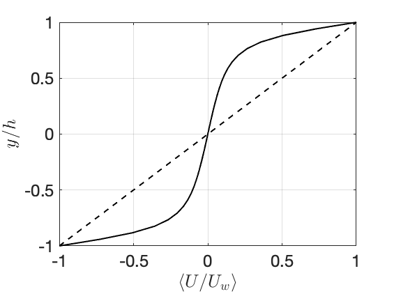
Figure 1: The mean turbulent velocity profile, $\overline{U}$, in a turbulent RNL simulation of pCf at $R=600$ in a channel with $L_{x}/h=1.75\pi$ and $L_{z}/h=1.2\pi$. The shear at the walls is $4.2~{}U_{w}/h$. The laminar Couette flow is shown for comparison (dashed).

From (5b) we obtain that the time mean state, $(\langle\mathbf{U}\rangle_{t},\langle C\rangle_{t})$ satisfies the equation

$$\overline{A}_{\alpha\gamma,k_{x}}(1)\overline{C}_{\gamma\beta,k_{x}}(1,2)+\overline{A}_{\beta\gamma,k_{x}}^{*}(2)\overline{C}_{\alpha\gamma,k_{x}}(1,2)=-\langle\tilde{A}_{\alpha\gamma,k_{x}}(1)\tilde{C}_{\gamma\beta,k_{x}}(1,2)+\tilde{A}_{\beta\gamma,k_{x}}^{*}(2)\tilde{C}_{\alpha\gamma,k_{x}}(1,2)\rangle_{t}~{},$$ (6)

where $\overline{C}$ is the time-mean second order cumulant, $\langle C\rangle_{t}$, $\overline{A}$ is the operator governing the linear evolution of fluctuations on the time-mean flow $\overline{U}(y)\hat{\mathbf{x}}\stackrel{{\scriptstyle\mathrm{def}}}{{=}}\langle\mathbf{U}\rangle_{t}$, and tilde denotes the departures from the time mean. We find that the r.h.s. of (6) does not vanish and consequently $(\langle\mathbf{U}\rangle_{t},\langle C\rangle_{t})$ is not a fixed point of the S3T SSD dynamics in post-transitional pCf turbulence. This time-mean state would have been a fixed point of the S3T SSD dynamics if the S3T SSD dynamics had a fixed point attractor (other than the laminar state), as is often the case in planetary turbulence. Instead, S3T dynamics demonstrates that this time-mean flow is unstable. Identification of this instability ensures that the ensemble statistical state cannot be associated with a stable flow to which it corresponds, as in the case of beta plane or pre-transitional boundary layer time mean states.

We have shown that the ensemble/time mean flow is not sustained by its consistent Reynolds stresses. However, it is a common practice to conjecture the existence of exogenous forces sustaining mean flows. Consistent with this common practice, we can study the S3T SSD stability properties of $(\langle\mathbf{U}\rangle_{t},\langle C\rangle_{t})$ by assuming that time-mean stresses sustain these states as equilibria and then determine the stability of these equilibria. This procedure might be realized physically by adding appropriate eddy viscosity to sustain the time-mean velocity as an equilibrium for the sake of studying the hydrodynamic stability properties of a flow, as has been done in the case of the Reynolds-Tiederman turbulent profile Reynolds and Tiederman (1967). We enforce that $(\langle\mathbf{U}\rangle_{t},\langle C\rangle_{t})$ form an equilibrium state by introducing stresses calculated from the simulation so that the SSD equilibrium conditions are satisfied:

$$\Delta\overline{U}_{\alpha}/R+\overline{F}_{\alpha}=0~{},\,$$ (7a)

$$\overline{A}_{\alpha\gamma,k_{x}}(1)\overline{C}_{\gamma\beta,k_{x}}(1,2)+\overline{A}_{\beta\gamma,k_{x}}^{*}(2)\overline{C}_{\alpha\gamma,k_{x}}(1,2)+\overline{Q}_{\alpha\beta,k_{x}}(1,2)=0~{},$$ (7b)

with both

$$\overline{F}_{\alpha}=-\frac{1}{2}\sum_{k_{x}}\mathop{\mathrm{Re}}\left(\partial_{\beta,1}\overline{C}_{\alpha\beta,k_{x}}(1,2)\right)_{1=2}-\langle\tilde{U}_{\beta}\partial_{\beta}\tilde{U}_{\alpha}\rangle_{t}+\partial_{\alpha}\langle P\rangle_{t}~{},$$ (8a)

$$\overline{Q}_{\alpha\beta,k_{x}}(1,2)=\langle\tilde{A}_{\alpha\gamma,k_{x}}(1)\tilde{C}_{\gamma\beta,k_{x}}(1,2)+\tilde{A}_{\beta\gamma,k_{x}}^{*}(2)\tilde{C}_{\alpha\gamma,k_{x}}(1,2)\rangle_{t}~{}.$$ (8b)

obtained from the simulations.

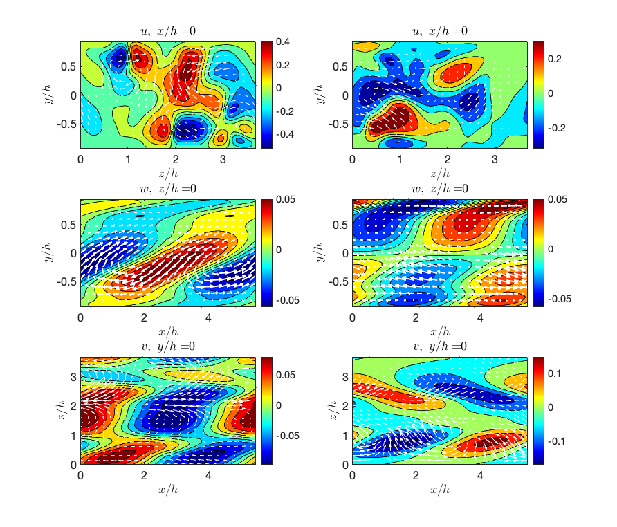
Figure 2: Columns showing snapshots of the velocity field with $k_{x}=2\pi h/L_{x}$ for fluctuations of the turbulent flow in an RNL simulation of pCf at $R=600$. The contour levels indicate the value of the fields. Top row: contours of $u^{\prime}$ velocity and vectors of $(w^{\prime},v^{\prime})$ on the $x/h=0$ plane. Maxima of $(u^{\prime},v^{\prime},w^{\prime})$ are $(0.46,0.13,0.08)$ (left panel) and $(0.40,0.21,0.12)$ (right panel). Middle row: contours of $w^{\prime}$ velocity and vectors of $(u^{\prime},v^{\prime})$ on the $z/h=0$ plane. Maxima of $(u^{\prime},v^{\prime},w^{\prime})$ are $(0.28,0.06,0.10)$ (left panel) and $(0.20,0.05,0.04)$ (right panel), Bottom row: contours of $v^{\prime}$ velocity and vectors of $(u^{\prime},w^{\prime})$ on the centerplane, $y/h=0$. Maxima of $(u^{\prime},v^{\prime},w^{\prime})$ are $(0.34,0.22,0.10)$ (left panel) and $(0.27,0.24,0.17)$ (right panel). Note that while the Reynolds stresses arising from averaging over these states are retained in $\overline{C}$, the phases determining the exact structures are not retained.

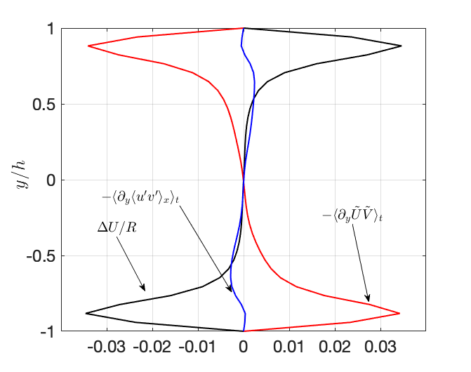
Figure 3: The force balance of the time-mean flow in pCf at $R=600$. The viscous force $R^{-1}d\overline{U}/dy^{2}$ is primarily balanced by the divergence of the time mean Reynolds stress of the fluctuations of the streamwise-mean flow $-\langle\partial_{y}\langle\tilde{U}\tilde{V}\rangle_{x}\rangle_{t}$. The divergence of the Reynolds stress of the streamwise-varying fluctuations, $-\langle\partial_{y}\langle u^{\prime}v^{\prime}\rangle_{x}\rangle_{t}$ is small.

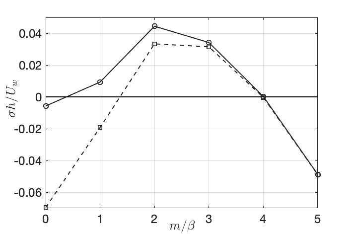
Figure 4: Growth rates of the most unstable S3T eigenmodes of the turbulent time-mean pCf mean flow shown in Fig. 1 as a function of the order of the spanwise harmonic, $m/\beta$, with $\beta=2\pi h/L_{z}$ the fundamental spanwise wavenumber. Solid line: growth rates of the antisymmetric in $y$ eigenfunctions. Dashed line: growth rates of the symmetric in $y$ eigenfunctions.

Having obtained in this way an equilibrium of the SSD we can determine its stability by considering the linear evolution of perturbations $\delta U$ and $\delta C_{k_{x}}$ in (5) (cf. Farrell and Ioannou (2012); Markeviciute and Kerswell (2023)). The perturbation equations that govern the $(\delta U,\delta C_{k_{x}})$ about the time-mean state $(\overline{U},\overline{C}_{k_{x}})$ are:

$$\partial_{t}\delta U_{\alpha}=-\overline{U}_{\beta}~{}\partial_{\beta}\delta U_{\alpha}-\delta U_{\beta}~{}\partial_{\beta}\overline{U}_{\alpha}+\Delta\delta U_{\alpha}/R-\partial_{\alpha}\delta P-\frac{1}{2}\sum_{k_{x}}\mathop{\mathrm{Re}}\left(\partial_{\beta,1}\delta C_{\alpha\beta,k_{x}}(1,2)\right)_{1=2}\ ,$$ (9a)

$$\partial_{t}\delta C_{\alpha\beta,k_{x}}(1,2)=\overline{A}_{\alpha\gamma,k_{x}}(1)~{}\delta C_{\gamma\beta,k_{x}}(1,2)+\overline{A}_{\beta\gamma,k_{x}}^{*}(2)~{}\delta C_{\alpha\gamma,k_{x}}(1,2)+$$

$$~{}~{}~{}~{}~{}~{}~{}~{}~{}~{}~{}~{}~{}~{}~{}~{}~{}~{}~{}~{}~{}\underbrace{\delta{A}_{\alpha\gamma,k_{x}}(1)~{}\overline{C}_{\gamma\beta,k_{x}}(1,2)+\delta{A}_{\beta\gamma,k_{x}}^{*}(2)~{}\overline{C}_{\alpha\gamma,k_{x}}(1,2)}_{S}\,$$ (9b)

$$\partial_{a}\delta U_{a}=0~{}~{},~{}~{}\hat{\partial}_{\alpha}(1)\delta C_{\alpha\beta,k_{x}}(1,2)=\hat{\partial}_{\beta}^{*}(2)\delta C_{\alpha\beta,k_{x}}(1,2)=0\ .$$ (9c)

The first equation (9a) governs the evolution of the perturbation of the first cumulant, while (9b) governs those of the second cumulant. The operator $\overline{A}_{k_{x}}$ is the operator that governs the evolution of perturbations about the time-mean flow $\overline{U}$, and $\delta{A}_{k_{x}}$ denotes the operator that governs the evolution of perturbations about the perturbed streamwise-mean flow $\delta{U}$. The term S in (9b), which describes the linear interaction between perturbations to the mean flow and the second cumulant of the unperturbed S3T equilibrium state, is responsible for the emergence of the new S3T instabilities. When $\overline{C}_{k_{x}}=0$ the first and second cumulant perturbation equations decouple and linear hydrodynamic stability of $\overline{U}$, which is determined from eigenalysis $\overline{A}_{k_{x}}$ in (9b), implies the linear S3T stability of the S3T state $(\overline{U},0)$. In general the $k_{x}$ in (9) are found to span only the small number of streamwise-vanumbers that comprise the active subspace sustaining the fluctuations and for which $\overline{C}_{k_{x}}\neq 0$. In the case discussed here the turbulent state is sustained with the single streamwise wavenumber $k_{x}=2\pi/L_{x}$. For the other $k_{x}$ that have $\overline{C}_{k_{x}}=0$, no investigation is necessary as S3T stability is implied from the hydrodynamic stability of the flow.

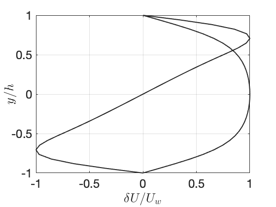
Figure 5: The structure of the $\delta U$ component of the first two least stable S3T spanwise constant ($m=0$) eigenmodes of the turbulent pCf, for which $\delta V=\delta W=0$. The time-mean flow when maintained to be a S3T equilibrium is stable to $m=0$ (spanwise constant) but unstable to spanwise varying perturbations, as shown in Fig. 4. The antisymmetric perturbation is the least stable with decay rate $\sigma=-0.006~{}U_{w}/h$ while the least stable symmetric perturbation has decay rate $\sigma=-0.07~{}U_{w}/h$. These stable $m=0$ modes do not correspond to the least stable eigenfunctions of the dynamics of relaxation to the time-mean flow, which are shown in Fig. 8.

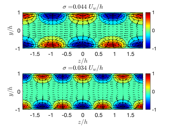
Figure 6: The structure of the first two most unstable eigenmodes of the turbulent pCf mean flow shown in Fig. 1 obtained by eigenanalysis of the operator governing the evolution of perturbations in the S3T equations. The most unstable eigenmode with spanwise wavenumber $m=2\beta$ (top panel) has growth rate $\sigma=0.04~{}U_{w}/h$, while the second most unstable eigenmode with $m=3\beta$ (bottom panel) has growth rate $\sigma=0.034~{}U_{w}/h$. The first cumulant component of the S3T eigenfunction has roll-streak structure. Shown are contours of the streamwise mean velocity, $\delta U$ (the contour level spacing is $0.2$), and velocity vectors of the components $(\delta V,\delta W)$ on the $(y/h,z/h)$ plane. Consistent with the lift-up mechanism, positive $\delta V$ is associated with negative $\delta U$. The maxima of $(\delta U,\delta V,\delta W)$ are proportional to $(1,0.23,0.26)$ in the $m=2\beta$ S3T eigenfunction and proportional to $(1,0.25,0.22)$ in the $m=3\beta$ S3T eigenfunction.

III Results

We consider a turbulent pCf at $R=600$ in a channel with $L_{x}/h=1.75\pi$, $L_{z}/h=1.2\pi$ in the quasi-linear approximation i.e. neglecting the fluctuation-fluctuation interaction in (1), as discussed in the previous section. The turbulent state supports fluctuations of only the single $k_{x}=2\pi h/L_{x}$ wavenumber.

We obtain the flow states for a period of $10^{4}~{}h/U_{w}$ time units with a discretization on $N_{y}=33$ grid points in $y$ and $N_{z}=48$ grid points in $z$. We have verified that the time period of the simulation is adequate for producing converged results . The time-mean turbulent flow $\overline{U}(y)$ is shown in Fig. 1, and the structure of two typical fluctuation states are shown in Fig. 2. $\overline{C}$ is the time-mean covariance of the velocities of the streamwise-varying flow obtained from all the individual snapshots that occur in the simulation. In the process of forming $\overline{C}$, the phase information associated with individual fluctuations is lost, while the time-mean Reynolds stresses that balance the time-mean flow are retained. Further insight into the maintenance of the time-mean flow can be obtained from the individual terms contributing to the maintenance. The time-mean flow force balance (7a) for the case of Couette turbulence simplifies to:

$$\underbrace{\frac{1}{R}\frac{d^{2}\overline{U}}{dy^{2}}}_{A}-\underbrace{\frac{d\langle\langle{u^{\prime}v^{\prime}}\rangle_{x}\rangle_{t}}{dy}}_{B}-\underbrace{\frac{d\langle{\tilde{U}\tilde{V}}\rangle_{t}}{dy}}_{C}=0~{},$$ (10)

with the viscous force (term A), by which the boundaries maintain the flow, being almost exclusively balanced by the time-mean Reynolds stress divergence of the streamwise constant time-varying velocity components (term C) (cf. Fig. 3), consistent with the mechanism of streak displacement by roll circulations in the 2D3C turbulence model of Gayme et al. (2010). It is remarkable that the component of the Reynolds stress divergence arising from the streamwise constant flow fluctuations (term C) so dominates the mean velocity force balance. This calls into question the adoption of spatially dependent diffusion as a mechanistic explanation for momentum fluxes maintaining time mean flows insofar as these fluxes are predicated on assuming they arise from small scale velocity correlations. The stress divergence arising from the time-mean eddy Reynolds stress of the streamwise varying components, obtained from the covariance $\overline{C}$ (term B), makes a minor contribution to the force balance (10).

While $\overline{C}$ is by necessity positive definite, being the time average of the instantaneous positive definite covariances of the fluctuations, this is not guaranteed for the time-mean $\overline{Q}$ obtained in (8b). We find that $\overline{Q}$ is non-positive definite, as was also found by Zare et al. (2017a) in a DNS of wall-bounded turbulence. This implies that if $\overline{Q}$ were to represent the spatial covariance of a stochastic excitation, this stochastic excitation must be temporally correlated (colored) Zare et al. (2017a).

The operator $\overline{A}_{k_{x}}$ in (7b) governing the evolution of perturbations about the time–mean flow $\langle\mathbf{U}\rangle_{t}\stackrel{{\scriptstyle\mathrm{def}}}{{=}}\overline{U}(y)$ is stable with the least damped mode at streamwise wavenumber $k_{x}=2\pi h/L_{x}$ decaying rate $\sigma=-0.11~{}U_{w}/h$. As is the case for the Reynolds-Tiederman mean-flow, the time-mean turbulent pCf flow, $\overline{U}(y)$, is far from a state of marginal hydrodynamic stability, violating the conjecture of Malkus that the time-mean flow is adjusted by turbulence to neutral stability, as occurs in Rayleigh-Bénard convection Malkus (1956); Reynolds and Tiederman (1967). However, here we show that the time-mean flow, although hydrodynamically stable, is unstable to the nonlinear instability revealed by the S3T dynamics.

To proceed with the S3T stability analysis of the turbulent state $(\langle\mathbf{U}\rangle_{t},\langle C\rangle_{t})$ we consider the stability of equations (9) governing cumulant perturbations about $(\langle\mathbf{U}\rangle_{t},\langle C\rangle_{t})$. The discretized linear operator that governs perturbations $(\delta U,\delta V,\delta W,\delta C_{k_{x}})$ in (9) has dimensionality $2N_{y}N_{z}(2N_{y}N_{z}+1)\times 2N_{y}N_{z}(2N_{y}N_{z}+1)$, which is $\approx 10^{7}\times 10^{7}$ in the model example we study, necessitating the use of the power method to obtain the fastest growing eigenvalues and eigenmodes of the equilibrium state, $(\langle\mathbf{U}\rangle_{t},\langle C\rangle_{t})$, as discussed in Farrell and Ioannou (2012); Farrell et al. (2017a). Due to the spanwise homogeneity of the background state the perturbation eigenmodes are harmonic in $z$ with mean flow components, $(\delta U_{m}(y),\delta V_{m}(y),\delta W_{m}(y))e^{imz}$, where $m$ is the spanwise wavenumber, with corresponding covariance $\delta C_{m,k_{x}}(y_{1},y_{2})e^{im(z_{1}-z_{2})}$. The growth rates of the most unstable S3T symmetric and antisymmetric in $y$ eigenfunctions as a function of $m$ are shown in Fig. 4. While the spanwise constant perturbations $(m=0)$ are S3T stable with structure shown in Fig. 5, the introduction of spanwise variation results in the time-mean flow being unstable to $m=1\beta,2\beta,3\beta$ S3T perturbations, with $\beta=2\pi h/L_{z}$ the fundamental spanwise wavenumber. The $(\delta U_{m}(y),\delta V_{m}(y),\delta W_{m}(y))e^{imz}$, component of the two most unstable eigenmodes of the perturbation S3T dynamics, with $m=2\beta$ and $m=3\beta$, are shown in Fig. 6. These unstable eigenmodes have the form of streamwise roll-streak (R-S) structures. This is also the case for the S3T eigenmodes of the laminar profile, but in contrast to the laminar flow S3T eigenmodes these R-S structures are confined to the near wall high shear regions of the mean turbulent profile. This universality of the structure of the S3T eigenfunctions reflects the universality in the mechanism of the S3T R-S instability Farrell and Ioannou (2012); Farrell et al. (2022). The two most unstable eigenmodes have real eigenvalues with growth rates $\sigma=0.04~{}U_{w}/h$ and $\sigma=0.034~{}U_{w}/h$ for spanwise wavenumber $m=2\beta$ and $m=3\beta$ respectively. Both eigenmodes are antisymmetric in $y$. Their symmetric counterpart eigenmodes are also unstable but with the smaller growth rates $\sigma=0.025~{}U_{w}/h$ and $\sigma=0.032~{}U_{w}/h$ respectively. As shown in Fig. 4, degeneracy of the growth rates between the symmetric and antisymmetric in $y$ modes is approached as $m$ increases. Degeneracy is expected as the velocity fields associated with the modes become more confined to their respective boundaries with either increase in $m$ or $R$.

We conclude that the S3T-SSD equilibrium state in pCf is unstable to perturbations with R-S structure and therefore can not be used to obtain the linear dynamics of perturbations from the mean statistical state by performing a perturbation analysis of the S3T SSD about the mean turbulent state. We note that the R-S unstable modes in turbulent flows depend only on the shear and similar unstable structures are expected to be found in other wall-bounded flows such as pPf and boundary layers. The fact that an ensemble mean state can be stable in ensemble dynamics while the same state is unstable to perturbation of each ensemble member individually can be understood by recalling the example of a mass-spring with random restoring force governed by the Mathieu equation Farrell and Ioannou (2002). Each realization of the state is unstable while the ensemble mean evolves as a stable harmonic oscillator with the average square frequency of the ensemble realizations. This example shows how the time-mean state may be an attractor for the ensemble mean but at the same time be a repeller for the perturbation dynamics as is the case for wall-turbulence.

IV Empirical determination of the effective linear dynamics of perturbations to the time-mean equilibrium state in a turbulent channel flow

Perturbation analysis of the S3T SSD equilibrium state provides comprehensive characterization of turbulent state stability in cases for which a stable S3T SSD equilibrium state exists. However, turbulent pCf and pPf lie on a transient chaotic attractor in statistical state space. Stability of the ensemble mean (or equivalently the time-mean) statistical state in these cases requires obtaining the perturbation dynamics averaged over the chaotic attractor. This can be accomplished by restricting attention to the time-mean flow component of the statistical state. As discussed in the introduction, IWCV found these first two eigenmodes and eigenvalues by averaging an ensemble of pPf DNS runs at $R_{\tau}=180$ in a channel with $L_{x}/h=8\pi$ and $L_{z}/h=4\pi$, $L_{y}/h=2$, which had been perturbed by the same initial streamwise flow perturbation, $\delta U(y)$. Here we obtain an approximate dynamical system in Langevin form for the relaxation of mean flow perturbations to the time-mean using an alternative method, called linear inverse modeling. The linear inverse model (LIM) obtains the effective dynamics of perturbations to the time-mean flow by observing the behavior of fluctuations to the time-mean velocity profile naturally occurring in the turbulence. In our study we first obtain using LIM the empirical dynamical system that governs the fluctuations from the streamwise-spanwise mean flow in the pCf simulation presented in the previous section, sampled every non-dimensional time unit, which we verified to adequately sample the temporal fluctuations of the streamwise and spanwise mean flow and also in a pPf at $R_{\tau}=180$ in a channel of $L_{x}/h=2\pi$ and $L_{z}/h=\pi$, $L_{y}/h=2$, with bulk velocity, $U_{b}$. The pPf data were obtained using a constant mass-flux DNS. The pPf and the pCf were integrated over a sufficient time ($6\times 10^{4}~{}h/U_{b}$ for the pPf and $10^{4}~{}h/U_{w}$ for the pCf) to obtain converged results as verified by using the data for half the interval.

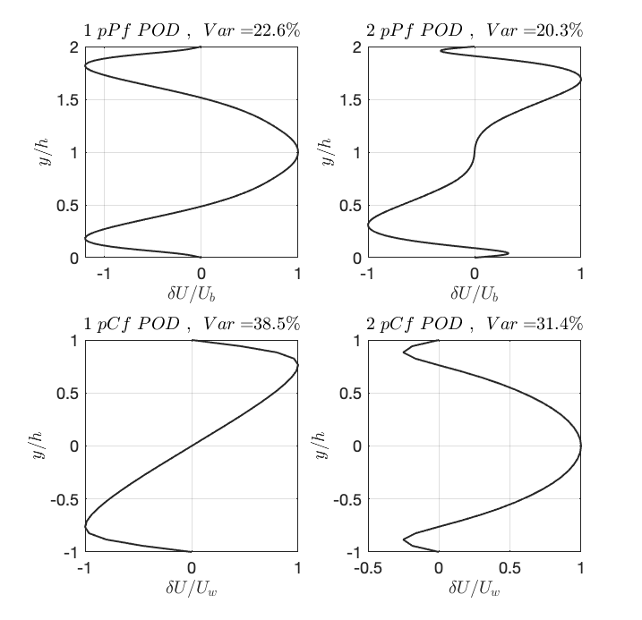
Figure 7: The structure of the first two POD modes of the mean flow fluctuations in pPf (top), and in pCf (bottom) Top left panel: the first POD mode of pPf accounts for $23\%$ of the energy of the fluctuations. Top right panel: the second POD of pCf accounts for $20\%$ of the energy of the fluctuations. Bottom left panel: the first POD mode of pCf accounts for $39\%$ of the energy of the fluctuations. Bottom right panel: the second POD of pCf accounts for $31\%$ of the energy of the fluctuations.

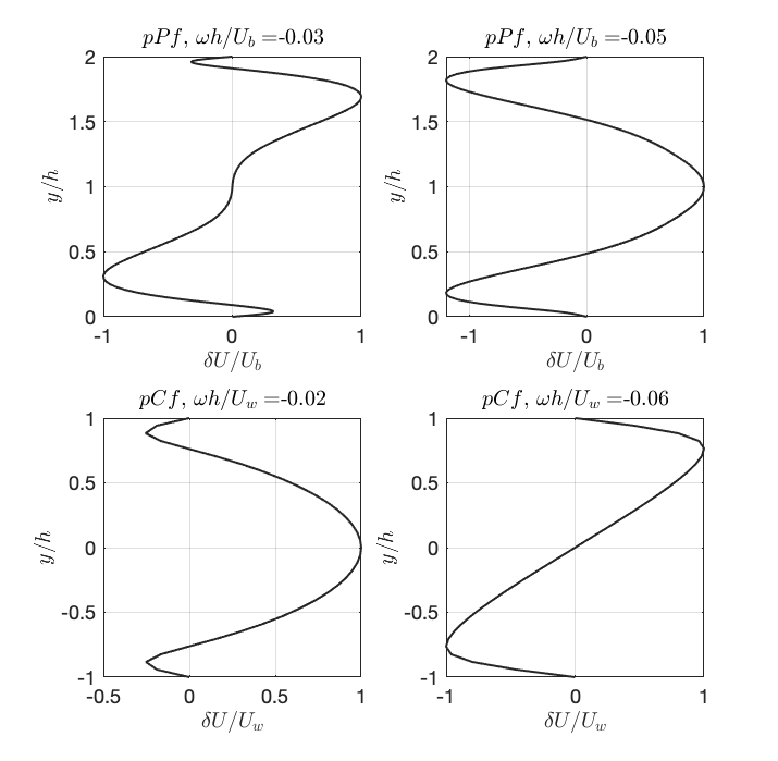
Figure 8: Structure of the eigenmodes of the $2\times 2$ LIM operator governing the relaxation of steamwise and spanwise mean flow fluctuations to the time-mean flow. Top left panel: the least damped mode in pPf is antisymmetric about the channel center and has eigenvalue $\omega h/U_{b}=-0.03$. Top right panel: the second least damped mode is symmetric and has eigenvalue $\omega h/U_{b}=-0.05$. Bottom left panel: the least damped mode in pCf is symmetric about the channel center and have eigenvalues $\omega h/U_{w}=-0.02~{}$. Bottom right panel: the second least damped mode is antisymmetric about the channel center and have eigenvalues $\omega h/U_{b}=-0.06$.

From the data we obtain the time series of the fluctuations $\delta U(y,t)$ about the time-mean flow with the asymptotic statistical symmetry of the time-mean flow, $\overline{U}(y)$, about the center-plane in the cross-flow direction in pPf and antisymmetry in pCf enforced by adding replicas of the mirror symmetric instantaneous mean flows about the center-plane in pPf and mirror antisymmetric replicas in pCf. Although the instantaneous realizations of the streamwise-spanwise averaged flow are not symmetrized, this symmetrizing operation results in the time-mean flow obtained from our finite data set, as well as in the time-mean statistical moments of the fluctuations to be exactly symmetric in pPf and antisymmetric in pCf. An important consequence of this symmetrization procedure is that it enforces in the data the known symmetries of the dynamics of pCf and pPf.

From the $\delta U(y,t)$ fluctuations we also obtain the time-mean fluctuation covariance:

$$C_{0}(1,2)=\langle\delta U(y_{1},t)\delta U(y_{2},t)\rangle_{t},$$ (11)

and the time-mean time-lagged covariances:

$$C_{\tau}(1,2)=\langle\delta U(y_{1},t+\tau)\delta U(y_{2},t)\rangle_{t}.$$ (12)

Due to the mean flow symmetrization procedure, the covariance $C_{0}$ and $C_{\tau}$ are symmetric about the $x-z$ plane at the channel center, i.e. they satisfy $C(y_{1},y_{2})=C(y_{1}^{s},y_{2}^{s})$, where $y_{i}^{s}$, $i=1,2$, is the symmetric coordinate of $y_{i}$ with respect to the channel center. The POD modes of the mean flow fluctuations are obtained from eigenanalysis of $C_{0}$. Due to the statistical symmetry reflected in $C_{0}$, the POD modes are necessarily either symmetric or antisymmetric.

LIM determines the best fit to our data by the linear stochastic system with Langevin form:

$$\frac{d~{}\delta U}{dt}=A~{}\delta U+\xi(t)~{},$$ (13)

where $\delta U$ is the column vector of the values at the $N_{y}$ wall-normal grid points, $A$ is the $N_{y}\times N_{y}$ matrix generator of the dynamics of fluctuations and $\xi(t)$ represents the spatial and temporal structure of the unresolved dynamics that are required to be parameterized as a zero mean temporally delta correlated Gaussian noise process satisfying $\langle\xi(y_{1},t)\xi(y_{2},t^{\prime})\rangle_{E}=\Xi(1,2)\delta(t-t^{\prime})$, with the full rank positive definite spatial covariance $\Xi(1,2)$ to be determined, along with the effective linear operator $A$, by inversion for the best fit to the dynamics (13). Note that LIM does not determine $\xi$, it determines only its spatial covariance $\Xi$. In LIM modeling the operator $A$ is discovered and is not assumed a priori to be either the operator $\overline{A}$ that governs perturbations about the mean flow, $\overline{U}$, or $\overline{A}$ modified by eddy viscosity as in the studies of Zare et al. (2017a); Hwang and Eckhardt (2020); Towne et al. (2020); Holford et al. (2023); Holford and Hwang (2023); Abootorabi and Zare (2023).

With a discretized representation the time lagged covariances of the velocity fluctuations, $C_{0}$ and $C_{\tau}$ in (11),(12), become matrices. Under the assumption that the stochastic excitation, $\xi$, in (13) is temporally white it can be shown (cf. DelSole (2004)) that:

$$C_{\tau}=e^{A\tau}C_{0}~{},\tau>0~{},$$ (14)

from which we obtain immediately that:

$$A=\frac{1}{\tau}\log(C_{\tau}C_{0}^{-1})~{},$$ (15)

The logarithm of any matrix $M$ that has a full basis of eigenvectors is $\log(M)=UDU^{-1}$, where $U$ is the matrix of the eigenvectors of $M$ and $D$ the diagonal matrix with diagonal elements the logarithms of the eigenvalues of $M$.

If there is an interval in $\tau$ for which, $\tau$ is both small enough to sample the dynamics and large enough that the correlation time of the fluctuations perturbing the eigenmodes can be represented by a Gaussian delta-correlated white noise process, so that in this interval $A$ is insensitive to $\tau$, then $A$ identifies the generator of the Langevin dynamics (13) rather than being merely the finite time map connecting $C_{0}$ to $C_{\tau}$ Papanicolaou and Kohler (1974); Penland and Sardeshmukh (1995); DelSole (2000); Penland (2019).

Boundedness of $C_{0}$ ensures the stability of the matrix $A$ and (13) requires that the covariance of the noise process $\Xi$ satisfies the Lyapunov equation:

$$AC_{0}+C_{0}A^{T}=-\Xi~{}.$$ (16)

$\Xi$ must be verified, for consistency, to be positive semi-definite given that it is the correlation of the forcing vector structures Penland and Sardeshmukh (1995). In this way LIM identifies the linear operator, $A$, that best fits the data while also determining the positive semi-definite spatial covariance, $\Xi$, of the effectively white temporal excitation of the fluctuations. By contrast, note that Zare et al. (2017a) constrain their stochastic model operator to be $\overline{A}$, which governs perturbations about the time-mean flow $\overline{U}$. The consequence is that the $\Xi$ that is obtained using (16) may not be positive definite. Such a non positive $\Xi$ is compatible with a set of stochastic models excited by colored noise Georgiou (2002); Zare et al. (2017a). To remove ambiguity among the members of this set Zare et al. (2017a) employ an optimization procedure. Moreover, Georgiou (2002); Zare et al. (2017b, a) show that each of these colored noise models with linear operator $A_{col}$ corresponds to a linear model with an appropriately modified operator $A_{white}$ driven by a white noise process. Importantly, LIM, removes the ambiguity in the choice of $A_{white}$ by determining the operator that best fits the data. LIM determines a unique operator by using the extra information encoded in the time lagged covariances, while Zare et al. (2017a) utilize only the information encoded in $C_{0}$. A clue to the underlying importance of identifying the unique LIM modified operator $A$ is offered in DelSole and Farrell (1996) who show that the modified $A$ in two-layer baroclinic turbulence model is the linear operator about the time mean flow, $\overline{A}$, corrected by the addition of a diffusion operator. This is consistent with the works of Hwang and Eckhardt (2020); Holford et al. (2023); Holford and Hwang (2023); Abootorabi and Zare (2023) who match the observed covariances by forcing white the linear operator about the mean flow, $\overline{A}$, modified by the inclusion of a diffusive operator with the Reynolds-Tiederman diffusion coefficient, indicating that the color of the stochastic forcing can be compensated for by inclusion of a parameterization of eddy viscosity in the form of a spatially varying diffusion. However, LIM allows going a step further by obtaining the unique form of this diffusion and by so doing providing an independent justification for the use of eddy diffusion as a parameterization of unresolved scales in turbulence models.

Another consideration for obtaining the effective dynamics is that the inverse of $C_{0}$ is ill-conditioned for data from a turbulent flow given that any finite time series can not resolve fluctuations of arbitrarily small scale and amplitude (cf. North et al. (1982)). Therefore, in order to obtain a converged dynamics we confine the representation of the dynamics to the subspace spanned by a set of dominant POD modes obtained from the covariance $C_{0}$ of the $\delta U$ fluctuations.

We first obtain the effective $2\times 2$ dynamical operator $A$ governing the dynamics of the fluctuations to the time-mean flow in the space of the top 2 POD modes in the pCf S3T and the pPf DNS, which account for $\approx 70\%$ and $\approx 40\%$ of the energy respectively. The top two POD modes are a symmetric and antisymmetric pair with structure shown in Fig. 7. We obtain the operator, $A$, from (15) and verify that the the noise covariance, $\Xi$, from (16) is positive definite. Insensitivity of the dynamics was obtained for time-lags around $\tau U_{b}/h=18$ in both pCf and pPf. The eigenmodes of $A$ are found to have the same structure as the POD modes used in the projection. The eigenvalue of the least damped antisymmetric mode is $\sigma=-0.03~{}U_{b}/h$ and that of the symmetric mode is $\sigma=-0.05~{}U_{b}/h$. The least damped eigenmode, shown in the top left panel of Fig. 8, is antisymmetric with respect to the channel center, consistently with the results of IWCV. However, our LIM analysis predicts a slower decay rate than theirs. The next in decay rate mode of $A$, shown in the top right panel of Fig. 8, is symmetric and its decay rate and structure are consistent with the least damped symmetric eigenmode of IWCV. The least damped eigenmodes in pCf are also real as shown in the lower panels of Fig. 8. The eigenvalue of the symmetric mode is $\sigma=-0.02~{}U_{w}/h$, and that of the asymmetric mode is $\sigma=-0.06~{}U_{w}/h$. While the POD modes have the same structure as the eigenmodes of $A$, in pPf the least damped antisymmetric mode of $A$ is excited less vigorously by $\Xi$, with the result that the dominant POD becomes the symmetric, although this is the more damped eigenmode of $A$. Similarly, in pCf the antisymmetric mode is favored by the excitation so that it accumulates more energy in the mean than does the least damped symmetric mode.

Coincidence of the modes of $A$ with the orthogonal POD modes imply the normality of $A$. Note that reflection symmetry of the ensemble dynamics about the cross-stream channel center requires that symmetric structures in the ensemble dynamics evolve to symmetric structures and antisymmetric to antisymmetric. Consequently, in the linear dynamics of the ensemble the eigenmodes of the dynamics are partitioned into a mutually orthogonal symmetric and antisymmetric set and the covariance of the excitation does not mix the symmetric and antisymmetric subspaces. An example of this property is the diagonal structure of both $A$ and of the spatial covariance, $\Xi$, in the $2\times 2$ projection of the dynamics. From this observation we also understand that any non-normality which may arise at higher truncations will be limited to the respective symmetric and antisymmetric subspaces (cf. Appendix for a discussion of the case of a $6\times 6$ truncation).

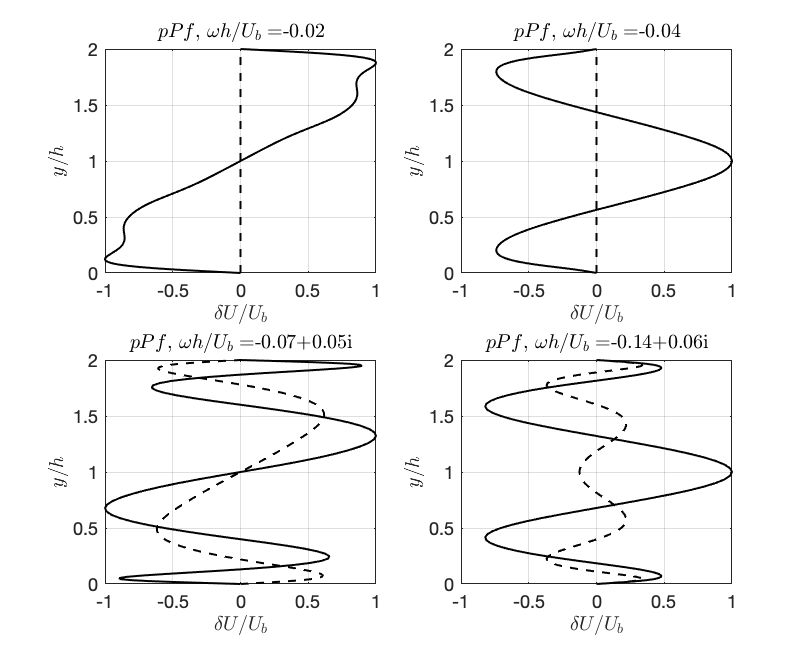
Figure 9: The structure of the real part (solid line) and the imaginary part (dashed line) of the 6 damped eigenmodes of the empirical operator $A_{6}$ of the pPf. Top left panel: the least damped mode is antisymmetric about the channel center and has eigenvalue $\omega h/U_{b}=-0.02$. Top right panel: the next least damped mode is symmetric and has eigenvalue $\omega h/U_{b}=-0.04$. Bottom left panel: the third and fourth least damped modes are antisymmetric about the channel center and have eigenvalues $\omega h/U_{b}=-0.07\pm 0.05i~{}$. Bottom right panel: the fifth and sixth least damped modes are symmetric about the channel center and have eigenvalues $\omega h/U_{b}=-0.14\pm 0.06i$. The structure of the complex valued eigenmodes periodically vary with a period of $T=O(100)~{}h/U_{b}$.

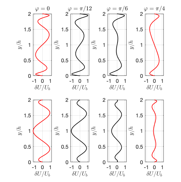
Figure 10: Evolution of the structure of the complex eigenmodes of $A_{6}$ over a quarter period of their oscillation. The decay is not included in this representation. Top panels: for the antisymmetric eigenmode shown in Fig. 9c with period $125~{}h/U_{b}$. Bottom panels: for the symmetric eigenmode in Fig. 9d. with period $105~{}h/U_{b}$.

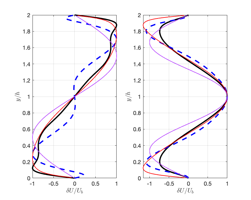
Figure 11: Comparison of the structure of the antisymmetric (left panel) and symmetric (right panel) least damped mode of $A_{6}$ (black line) and of the corresponding modes in diffusive models. With red lines: the least decaying modes of the Reynolds-Tiederman eddy-viscosity model at $R_{\tau}=180$ (red). With purple solid lines: the least damped modes of the purely diffusive model with $R=2767$, corresponding to the laminar Reynolds number associated with $R_{\tau}=180$. The structure of the top POD modes is indicated with the dashed blue line. The departure of the $A_{6}$ modes from the associated POD mode indicates the degree of non-normality of the ensemble dynamics of relaxation to the mean and the degree of non-commutation of $A_{6}$ with $\Xi_{6}$.

Given the constraints on the dynamics arising from projections onto a single symmetric and a single antisymmetric POD mode, we consider higher order truncations. As already discussed, non-orthogonality can only emerge among the antisymmetric (or symmetric) eigenmodes of $A$ and other antisymmetric (or symmetric) eigenmodes of $A$. We demonstrate the emergence of non-normality in the dynamics in the case of the pPf by retaining in the dynamics the first 6 POD modes, which together account for $90\%$ of the mean-flow fluctuation energy. The results that we present do not appreciably change when the dimension of the retained POD modes is increased to 10. With 6 POD modes we find that $\tau=18~{}h/U_{b}$ produces a $\tau$-insensitive dynamical operator, $A_{6}$, and converged positive definite covariance, $\Xi$ (cf. Appendix for details). We conclude that in pPf the dynamics of perturbations to the time mean flow is generated by the matrix $A_{6}$ the eigenvalues of which are: $-0.02~{}U_{b}/h$, $-0.04~{}U_{b}/h$, $(-0.07\pm 0.05i)~{}U_{b}/h$, $(-0.14\pm 0.06i)~{}U_{b}/h$. The least damped eigenmode, shown in the top left panel of Fig. 9, is antisymmetric with respect to the channel center, consistent with the results of IWCV. However, our LIM analysis predicts a slower decay rate than theirs for the same $R_{\tau}$, allbeit in a channel of 1/4th size. The next in decay rate mode of $A_{6}$ is symmetric in structure with decay rate and structure consistent with the real part of the least damped symmetric eigenmode of IWCV. Although the first two eigenvalues of $A_{6}$ are real and represent the ensemble mean relaxation of structures of fixed form to the mean flow with time scales of $\approx 50~{}h/U_{b}$ and $\approx 25~{}h/U_{b}$ respectively, the remaining eigenmodes represent a damped oscillatory relaxation to the mean flow which oscillates between the real part and the imaginary part of the eigenmode over $\approx 100~{}h/U_{b}$, which is the characteristic period of the SSP cycle Hamilton et al. (1995). The evolution of the oscillating structure of the two complex eigenmodes is shown in Fig. 10.

The operator $A_{6}$ governing the dynamics is non-normal in the energy norm, as was conjectured by IWCV. The inner product of the eigenmodes shows that there are substantial projections among modes in both the symmetric and antisymmetric subspace and therefore the operator $A_{6}$ is substantially non-normal (cf. Appendix). The difference in structure between the eigenmodes and the POD modes reflects both the degree of non-normality of $A_{6}$ and the degree of non-commutation of $A_{6}$ with the excitation covariance $\Xi_{6}$ North (1984); Monahan et al. (2009); in general the POD modes in this Langevin system coincide with the eigenmodes of the linear operator $A$ when $A$ is normal and $[A,\Xi]=0$ (see Appendix). Fig. 11 shows that the structure of the eigenmodes departs appreciably from that of the associated POD modes. Moreover, non-normality of the dynamics is not consistent with a strictly diffusive process. However, it could be argued that the flow relaxes through the smoothing that results from the advection induced by the random action of the streamwise roll motions over the ensemble realizations of the flow and therefore the dynamics might be modeled as a diffusion with an appropriate coefficient assuming diffusion to be broadly conceived as any transport process resulting in a linear flux/gradient relation. To evaluate this hypothesis we compare the decay rates and structures of the eigenmodes predicted by an eddy viscosity model in which the mean flow perturbations are governed by

$$\frac{\partial\delta U}{\partial t}=\frac{\partial}{\partial y}\left(\nu_{E}(y)\frac{\partial\delta U}{\partial y}\right)~{},$$ (17)

with $\nu_{e}(y)$ an eddy viscosity coefficient. We will obtain the eigenvalues and eigenmodes in the case of simple diffusion with $\nu_{e}(y)=1/R$, with $R$ the laminar value of the Reynolds number, and the eddy viscosity that sustains the Reynolds & Tiederman Reynolds and Tiederman (1967) turbulent profile in a pPf channel with walls at $y=0$ and $y=2$. This profile is maintained by $\nu_{E}=(1+E(y))/R_{\tau}$ and $E(y)=\left(\sqrt{1+e^{2}}-1\right)/2$, where

$$e(y)=\frac{kR_{\tau}}{3}(1-(y-1)^{2})(1+2(1+(y-1)^{2})(1-\exp(-R_{\tau}(1-|y-1|)/A))~{},$$ (18)

with $K=0.525$ and $A=37$ as is appropriate for $R_{\tau}=180$. The least damped modes comprise a symmetric/antisymmetric pair, shown in Fig. 11. These modes are qualitatively similar to the modes obtained by LIM (cf. Fig. 11), but lack the detailed structure of the LIM or IWCV eigenmodes. Also, the decay rates of the two least damped modes are underpredicted by a factor $O(10)$ in the case of the molecular viscosity parameterization, and overpredicted by a factor of $O(10)$ in the case of the eddy viscosity parameterization that produces the Reynolds-Tiederman turbulent mean flow. These results suggest caution in interpreting the eddy viscosity required to produce the observed mean flow to be an equivalent diffusion that is at the same time acting on smaller scale structures. This is consistent with the findings of Russo and Luchini Russo and Luchini (2016).

LIM not only predicts the decay rate of perturbations to the time-mean flow but also predicts the variance of the perturbations around the decaying trajectory. The Langevin dynamics of the fluctuations obtained using LIM predicts a slight non-normal modification of the exponential decay of the modes to the time-mean opposed by diffusive spreading of the modes away from the time-mean produced by the stochastic forcing. The resulting PDF for the case of the $2\times 2$ dynamics obtained by LIM, which is normal implying no mode coupling, can be obtained from the companion Fokker-Planck equation:

$$\frac{\partial f}{\partial t}=-\omega\frac{\partial(xf)}{\partial x}+D\frac{\partial^{2}f}{\partial x^{2}}~{},$$ (19)

in which $f$ is the perturbed mode probability distribution, $x$ is the value of the coefficient of the projection on the associated POD mode, and $D$ is the diffusion coefficient equal to half the corresponding diagonal element of the covariance, $\Xi$, that excites the associated eigenmode of $A$ with stable real eigenvalue, $\omega$ . The perturbed mode distribution drifts back to the equilibrium under the influence of $\omega$ around which it maintains the predicted asymptotic distribution:

$$f(x)=\frac{\sqrt{-\omega}}{\sqrt{2\pi D}}\exp\left(\frac{\omega}{2D}x^{2}\right)~{},~{}~{}(\omega<0).$$ (20)

The probability distributions for these cases is plotted in Fig. 12. Also shown is the PDF obtained by binning the simulation data. Clearly, even this $2\times 2$ LIM dynamics obtained by projection on the first 2 POD modes suffices to predict the observed distribution of the fluctuations.

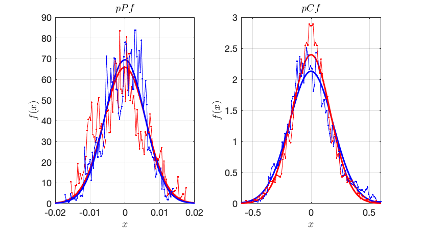
Figure 12: Comparison between the LIM prediction and the observed PDF of fluctuations. The predicted PDF was obtained from the $2\times 2$ LIM. Left panel: for the pPf shown separately are the probability of projection on the symmetric POD (red) and the antisymmetric POD (blue). The symmetric mode has $\omega=-0.05$ and $D=1.8e-06$ and the antisymmetric has $\omega=-0.03$ and $D=0.85e-06$. Right panel: for the pCf, the symmetric mode has $\omega=-0.02$ and $D=0.6e-03$ and the antisymmetric mode has $\omega=-0.06$ and $D=1.85e-03$.

V Conclusions

It is accepted that the ensemble mean state is a fixed point of the ensemble dynamics to which almost all perturbations relax. It is also believed that sufficiently small perturbations relax following a stable linear dynamics. Recently IWCV obtained from a perturbed DNS the dominant modes underlying this stable linear dynamics using an ensemble method. However, the interpretation of ensemble dynamics is not straightforward and in this case the ensemble converges to an unstable repeller of the realization dynamics rather than to a stable fixed point. This is common in ensemble dynamics, although apparently paradoxical, as the example of the mass-spring with random restoring force governed by the Mathieu equation discussed in the Formulation section demonstrates.

It is generally accepted that the ensemble mean state is stable in the sense of linear hydrodynamic stability. However, when account is taken of a set of nonlinear instabilities identified by S3T-SSD, it is a repeller in pPf and pCf turbulence. In this paper we have examined the implications of this ensemble mean flow instability for the dynamics of relaxation to the ensemble mean state. In the S3T SSD the mean state is the streamwise average, the fluctuations are the streamwise varying components, and the fluctuation-fluctuation interactions are neglected. A close approximation to the mean flow and the fluctuation covariance in the S3T SSD is obtained from a quasi-linear integration of pCf dynamics from which it is verified that the time-mean turbulent state is not a fixed point of the S3T dynamics. Moreover, even if the mean turbulent state is enforced to be an equilibrium, this equilibrium is S3T unstable.

It should be noted that this result applies to the case of post-transitional wall-bounded turbulence and should be contrasted to the case for pre-transitional pCf and to the turbulence that occurs in barotropic or baroclinic quasi-geostrophic models of planetary turbulence, in which often the time-mean turbulent state is a stable fixed point of both the ensemble and the S3T SSD dynamics. The SSD fixed point in these cases corresponds, in both the ensemble SSD and the S3T SSD, to the statistical mean turbulent state, both the ensemble mean and perturbations (up to second order Gaussian approximation in the case of the S3T SSD). This fixed point solution in the case of the planetary turbulence exhibits the characteristic structure of alternating zonal jets Farrell and Ioannou (2008, 2009b, 2017) together with the associated covariances which support the jets by upgradient Reynolds stresses Salyk et al. (2006). A familiar physical example of this SSD equilibrium is the zonal jets of Jupiter that have been demonstrated to have a fixed structure over at least decadal periods Ingersoll et al. (2004).

The difference between wall-bounded post-transitional turbulence and its pre-transitional and planetary counterparts is that in the latter cases the S3T SSD has an attracting fixed point which coincides with the ensemble/time-mean state of the turbulence and standard methods of eigenanalysis can be used to obtain the dynamics of perturbations back to the ensemble/time-mean state. In wall-turbulence the S3T trajectory lies on a transient chaotic attractor and eigenanalysis of the S3T state can not be performed to obtain the perturbation dynamics. However, nothing essential is lost as the perturbation dynamics can be obtained by averaging over the transient S3T attractor, which was accomplished using LIM analysis. Our results lend credence to the concept that the fundamental attractor of the turbulent state is identified by the S3T attractor in cumulant variables. When this attractor is visualized in velocity variables it corresponds to a turbulent state with the mean state containing the majority of the energy accompanied by a multivariate elliptical PDF of fluctuations in its immediate vicinity accounting for the remaining energy. Similarly, if we visualize the DNS attractor in velocity variables we find the majority of the energy to be contained in the mean flow with fluctuations in the vicinity accounting for the remaining energy. The S3T attractor identifies the structure and dynamics of this fundamental entity of the turbulence as comprising the first and second cumulants as the fundamental variables, visualized as the mean flow and the surrounding elliptical perturbation distribution, and their interaction as controlling the evolution of the turbulent state in the fundamental SSD variables or equivalently as visualized in velocity variables. Therefore the S3T SSD predicts both the underlying structure and evolution of the turbulent state in phase space.

Similarity between the dynamics of perturbations to the ensemble mean state in S3T SSD simulations, in which the structure and dynamics on the SSD attractor have been explicitly identified, and DNS suggests that the existence of the SSD transient attractor and the concept of averaging over this attractor in order to identify the dynamics of perturbations to the statistical time-mean state extends to DNS. These results suggest that the essentially complete characterization of turbulence in the S3T SSD, and especially the identification of a chaotic attractor in the phase space of the statistical state variables, can be profitably exploited to gain further insight into the dynamics of NS turbulence.

VI Appendix: The structure of the relaxation dynamics produced by LIM on 6 POD modes

When the mean-flow velocity fluctuations are projected on the top 6 POD modes ordered according to their contribution to the mean fluctuation energy, LIM identifies that the fluctuations are governed by operator:

$$A_{6}=\left(\begin{array}[]{cccccc}-0.021&0&0&0.048&0&-0.117\\ 0&-0.023&-0.040&0&-0.004&0\\ 0&0.024&-0.050&0&0.044&0\\ -0.035&0&0&-0.076&0&0.200\\ 0&-0.043&-0.038&0&-0.091&0\\ 0.024&0&0&-0.046&0&-0.239\end{array}\right)~{},$$

and are excited by a temporally delta-correlated white noise forcing with spatial covariance:

$$\Xi_{6}=10^{-5}\left(\begin{array}[]{cccccc}0.177&0&0&0.036&0&0.013\\ 0&0.15&0.04&0&0.15&0\\ 0&0.04&0.302&0&0.05&0\\ 0.036&0&0&0.34&0&-0.094\\ 0&0.15&0.05&0&0.26&0\\ 0.013&0&0&-0.094&0&0.475\end{array}\right)~{}.$$

Note that the POD modes, when ordered in variance, have the following symmetry: s,a,a,s,a,s respectively (“s” denotes symmetry about the $x-z$ center plane at $y/h=1$ and “a” antisymmetry). Because of the statistical symmetry of the fluctuations, interactions among them are restricted to the respective symmetric and antisymmetric subspaces, and consistently the only non-zero entries in the $A_{6}$ and $\Xi_{6}$ matrices are either in the coordinates of the symmetric modes corresponding to the POD modes 1,4,6 or those of the antisymmetric corresponding to the POD modes 2,3,5 .

That the dynamics is non-normal in the energy inner product can be ascertained by calculating the projections among the eigenmodes indicated by the matrix of the inner product, $u^{\dagger}u$:

$$u^{\dagger}u=\left(\begin{array}[]{cccccc}1&0&0.3+0.3i&0.3-0.3i&0&0\\ 0&1&0&0&0.7+0.05i&0.7-0.05i\\ 0.3-0.3i&0&1&0.3-0.3i&0&0\\ 0.3+0.3i&0&0.3+0.3i&1&0&0\\ 0&0.7-0.05i&0&0&1&0.9+0.05i\\ 0&0.7+0.05i&0&0&0.9-0.05i&1\end{array}\right)~{}.$$

Here the eigenmodes are ordered increasing in decay rate. The symmetric eigenmodes are 2,5,6 and the antisymmetric are 1,3,4 and it can be seen, as expected by the statistical symmetry of the dynamics, that non-normal interaction is confined to the mutually orthogonal symmetric and antisymmetric subspaces.

Non-normality of $A_{6}$ and non-commutation between $A_{6}$ and $\Xi_{6}$ results in the POD modes of the Langevin dynamics differing from the eigenmodes of the operator of the dynamics, $A_{6}$, as discussed by North (1984); Monahan et al. (2009). However, the statistical symmetry of the dynamics still constrain the POD modes to lie in the mutually orthogonal symmetric and the antisymmetric subspaces of the eigenmodes. The commutator between $A_{6}$ and $\Xi_{6}$ is:

$$[A_{6},\Xi_{6}]=\left(\begin{array}[]{cccccc}0.001&0&0&0.021&0&-0.044\\ 0&0.003&0.005&0&0.006&0\\ 0&0.004&0.007&0&0.004&0\\ 0.009&0&0&-0.026&0&0.015\\ 0&-0.008&0.006&0&-0.01&0\\ -0.015&0&0&0.022&0&0.025\end{array}\right)~{}.$$

The requirement for identity of the POD modes with the modes of the operator in general Langevin dynamics can be immedialtely seen as follows: the POD modes are the eigenmodes of the fluctuation covariance $C$, which is given in Langevin systems by $\int_{0}^{\infty}dt~{}e^{At}\Xi e^{A^{\dagger}t}$. Therefore, the eigenmodes of $C$ coincide with the eigenmodes of $A$ if $[A,A^{\dagger}]=0$, i.e. $A$ is normal, and $[A,\Xi]=0$, i.e. the forcing does not mix the eigenmodes of $A$.