DistHD: A Learner-Aware Dynamic Encoding Method for Hyperdimensional Classification

Abstract

The Internet of Things (IoT) has become an emerging trend that connects heterogeneous devices and enables them with new capabilities. Many applications exploit machine learning methodology to dissect collected data, and edge computing was introduced to enhance the efficiency and scalability in resource-constrained computing environments. Unfortunately, popular deep learning algorithms involve intensive computations that are overcomplicated for edge devices. Brain-inspired Hyperdimensional Computing (HDC) has been considered a promising approach to address this issue. However, existing HDC methods use static encoders, and thus require extremely high dimensionality and hundreds of training iterations to achieve reasonable accuracy. This results in a huge loss of efficiency and severely impedes the application of HDC algorithms in power-limited machines. In this paper, we propose $\mathsf{DistHD}$, a novel HDC framework with a unique dynamic encoding technique consisting of two parts: top-2 classification and dimension regeneration. Our top-2 classification provides top-2 labels for each data sample based on cosine similarity, and dimension regeneration identifies and regenerates dimensions that mislead the classification and reduce the learning quality. The highly parallel algorithm of $\mathsf{DistHD}$ effectively accelerates the learning process and achieves the desired accuracy with considerably lower dimensionality. Our evaluation on a wide range of practical classification tasks shows that $\mathsf{DistHD}$ is capable of achieving on average $2.12\%$ higher accuracy than state-of-the-art (SOTA) HDC approaches while reducing dimensionality by $8.0\times$. It delivers $5.97\times$ faster training and $8.09\times$ faster inference than SOTA learning algorithms. Additionally, the holographic distribution of patterns in high dimensional space provides $\mathsf{DistHD}$ with $12.90\times$ higher robustness against hardware errors than SOTA DNNs. $\mathsf{DistHD}$ has been open-sourced to enable future research in this field.

I Introduction

The Internet of Things (IoT) has recently become an emerging trend for its extraordinary potential to connect various heterogeneous smart sensors and devices and enable them with new capabilities. Many IoT applications exploit machine learning (ML) algorithms to dissect collected data and perform learning and cognitive tasks. However, the excellent learning quality of popular ML approaches, including deep neural networks (DNNs), often comes at the expense of high computational and memory requirements, involving millions of parameters that need to be iteratively refined over multiple time periods [1]. One common approach is to leverage cloud computing by sending data from the network edge to the centralized location in the cloud. Unfortunately, this potential solution results in significant efficiency loss, multiple scalability issues, and serious privacy concerns [2]. Edge computing, a novel computing paradigm performing calculations in proximity to data sources, has since been introduced to address these issues. However, accommodating the high resource requisite of traditional learning methodologies on less powerful computing platforms remains a critical challenge to surmount [1]. Considering the increasingly massive amount of information nowadays, the power and memory limitations of embedded devices, and the potential instabilities of IoT systems, a more lightweight, efficient, and robust learning algorithm is of absolute necessity [3].

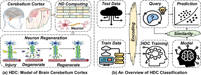
Figure 1: An Overview of Brain Cerebellum Cortex and HDC Classification

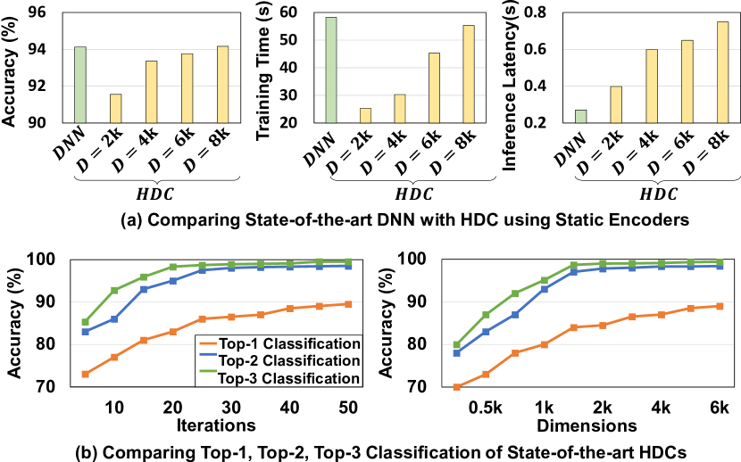
Figure 2: Motivation for Dynamic Encoding and Top-2 Classification

In contrast to traditional artificial intelligence methodologies, HDC is considered a promising learning approach for less powerful computing platforms for its (i) high computational efficiency ensuring real-time learning [4], (ii) strong robustness to noise – a key strength for IoT systems [5], and (iii) lightweight hardware implementation enabling efficient execution on edge device [6]. As demonstrated in Fig. 1(a), HDC is motivated by the neuroscience observation that the cerebellum cortex in the human brain is capable of effortlessly and efficiently processing memory, perception, and cognition information without much concern for noisy or broken neuron cells. Closely mimicking the information representation and memorization functionalities of human brains, HDC encodes low-dimensional inputs to hypervectors with $10^{4}$ or more elements to perform various learning tasks [7] as shown in Fig. 1(b). HDC then conducts highly parallel and well-defined operations and has been proven to achieve high-quality results in classification and regression learning tasks with comparable accuracy to state-of-the-art (SOTA) DNNs and SVMs. Additionally, the notably faster convergence and higher efficiency offered by HDC provide a powerful solution for today’s embedded devices with limited storage, battery, and resources [4, 6, 5].

Despite the enormous success in the development of HDC, as demonstrated in Fig. 2(a), existing HDC algorithms require extremely high dimensionality ($D$) to outperform DNNs. Consequently, not only is the learning efficiency considerably lowered with large numbers of unnecessary computations involved, but the system efficiency is also compromised due to the increased data size and communication cost [5]. This severely impedes the feasibility and scalability of HDC in resource-constrained computing devices, especially for learning tasks including massive amounts of data and requiring real-time analysis. We observed that one of the main causes is that the encoding module of existing HDC approaches lacks the capability to utilize and adapt to information learned during the training process. On contrary, as demonstrated in Fig.1(a), neurons in human brains dynamically change and regenerate all the time and provide more useful functionality when they learn new information [8]. While the goal of HDC is to exploit the high-dimensionality of randomly generated base hypervectors to represent the information as a pattern of neural activity, it remains challenging for existing HDC algorithms to support a similar behavior as brain neural regeneration.

One interesting observation of SOTA HDC approaches is that they provide considerably higher accuracy and faster convergence for top-2 classification than top-1 classification, as shown in Fig. 2(b). Here we define a top-k classification for a given data point as correct if the true label is one of the k most similar classes selected. Additionally, the accuracy difference between top-2-classification and top-3 classification is noticeably smaller than that between top-1 classification and top-2-classification. Based on this observation, in this paper, we propose $\mathsf{DistHD}$, a new HDC framework with an innovative encoding technique that utilizes and adapts to information learned from every training iteration. $\mathsf{DistHD}$ aims at identifying dimensions that mislead the classification and decrease the learning accuracy, and regenerating them for a more positive impact on the learning quality. The main contributions of the paper are listed below:

• We propose a novel dynamic encoding technique for HDC combining top-2 classification and dimension regeneration optimizations. To the best of our knowledge, $\mathsf{DistHD}$ is the first HDC algorithm with a dynamic encoding module that identifies and regenerates dimensions hurting the classification accuracy to enhance learning quality. $\mathsf{DistHD}$ achieves on average $2.12\%$ higher classification accuracy than SOTA HDCs while reducing the number of needed dimensions by $8.0\times$. This ensures accurate performance for classification tasks on resource-constrained devices.

• The highly parallel and matrix-wise operations of $\mathsf{DistHD}$ ensures a considerable acceleration for performing classification tasks in both high-performance and resource-constrained computing environments. $\mathsf{DistHD}$ delivers $5.97\times$ faster training than SOTA DNNs and $8.09\times$ faster inference than SOTA HDC algorithms.

• The holographic distribution of patterns in high-dimension space enables $\mathsf{DistHD}$ with notably higher robustness. Our proposed model demonstrates on average $12.90\times$ higher robustness against hardware errors than SOTA DNNs. This ensures the effective execution of classification tasks on noisy IoT devices.

The rest of the paper is organized as follows: in Section II, we briefly introduce recent works in edge-based learning and HDC. We then explain our proposed methodology in detail in Section III, and evaluate our model in terms of accuracy, efficiency, and robustness against noise in Section IV. We conclude our work in Section V.

II Related Works

II-A IoT and Edge-based Learning

The rapid development of IoT has engendered a number of innovative works on the feasibility and scalability of edge-based learning. Prior works have demonstrated that machine learning algorithms (including DNNs) can possibly be customized for learning on edge computing devices. Various frameworks and libraries have been developed for learning on the edge, including TinyML [9], TensorFlow Lite [10], edge-ml [11], X-Cube-AI [12], etc. These frameworks are all machine learning or deep learning based tools. Many of these learning methods require a large number of training samples and long training cycles, and may not meet the tight constraints of ultra-low-power edge platforms. On the other hand, people propose techniques that improve learning efficiency on the edge, leveraging learning structures and target platform properties. Representative examples include split computing [13], federated learning [14, 15], knowledge distillation [16], etc. These techniques are orthogonal to our method and can potentially be integrated with our learning solution.

II-B Hyperdimensional Computing

Prior studies have exhibited enormous success in various applications of HDCs, such as brain-like reasoning [17], bio-signal processing [18], and human-activity recognition [19]. A few endeavors have been made towards developing novel architecture to accelerate HDC inference tasks [20]. However, popular HDC methods use pre-generated static encoders and thus require extremely high dimensionality to achieve acceptable accuracy [21]. NeuralHD [7], a recently proposed dynamic encoding approach, successfully compressed dimensionality by eliminating dimensions with minor impacts on distinguishing patterns. However, its proposed model takes a significantly longer time than SOTA HDC algorithms [6] to reach convergence, and it lacks an effective technique to enhance its encoding module with information learned during the training process. In contrast, we propose $\mathsf{DistHD}$, aiming at fully exploiting information learned from each iteration and achieving adequate accuracy with much faster convergence and lower dimensionality.

III Methodology

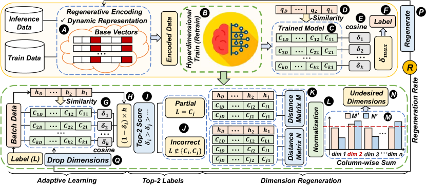
Figure 3: An Overview of $\mathsf{DistHD}$ Workflow

Popular HDC algorithms use static encoding techniques where the pre-generated base vectors lack the capacity to adapt to information learned during the training process. The goal of our proposed $\mathsf{DistHD}$ is to effectively exploit information learned from each training iteration to identify dimensions that reduce the learning quality and regenerate them. As demonstrated in Fig. 3, $\mathsf{DistHD}$ starts with encoding data points into high-dimensional space with existing encoding methods depending on the data type $(\leavevmode\hbox to7.69pt{\vbox to7.69pt{\text{[drawing]}}})$. $\mathsf{DistHD}$ then conducts two innovative steps, top-2 classification and dimension regeneration, to enable its encoding module and base vectors with adaptivity to each partially trained model. In each iteration of top-2 classification, $\mathsf{DistHD}$ first applies a highly efficient adaptive learning algorithm over the encoded data $(\leavevmode\hbox to7.4pt{\vbox to7.4pt{\text{[drawing]}}})$, and then utilizes the partially trained model to compute the top two most similar classes for each data point $(\leavevmode\hbox to5.49pt{\vbox to5.49pt{\text{[drawing]}}})$. In dimension regeneration, we calculate two distance matrices $(\leavevmode\hbox to7.91pt{\vbox to7.91pt{\text{[drawing]}}})$ based on results from the top-2 classification, and identify $(\leavevmode\hbox to7.69pt{\vbox to7.69pt{\text{[drawing]}}})$ and eliminate $(\leavevmode\hbox to9.3pt{\vbox to9.3pt{\text{[drawing]}}})$ undesired dimensions that mislead the classification tasks. To further improve the learning quality, we regenerate those dimensions $(\leavevmode\hbox to7.2pt{\vbox to7.2pt{\text{[drawing]}}})$ for a more positive impact on the classification. Note that all the operations in this section can be done in a highly parallel matrix-wise way, as multiple training samples can be grouped into a matrix of row hypervectors.

III-A HDC Preliminaries

Motivated by the high-dimensional information representation and memorization functionalities in human brains, HDC maps inputs onto hyperdimensional space as hypervectors $(\leavevmode\hbox to7.69pt{\vbox to7.69pt{\text{[drawing]}}})$, each of which contains thousands of elements. One unique property of the hyperdimensional space is the existence of a large number of nearly orthogonal hypervectors, enabling highly parallel operations such as similarity calculations, bundlings, and bindings. Mathematically, consider random bipolar hypervectors ${\mathcal{H}}_{1}$ and ${\mathcal{H}}_{2}$ with dimension $\mathcal{D}$, i.e., ${\mathcal{H}}_{1},{\mathcal{H}}_{2}\in\{-1,1\}^{\mathcal{D}}$, when $\mathcal{D}$ is large enough, the dot product ${\mathcal{H}}_{1}\cdot{\mathcal{H}}_{2}\approx 0$. Similarity: calculation of the distance between the query hypervector and the class hypervector (noted as $\delta(\cdot,\cdot)$). For real-valued hypervectors, a common measure is cosine similarity, i.e.

$$\delta({\mathcal{H}},{\mathcal{C}_{l}})=\frac{{\mathcal{H}}\cdot{\mathcal{C}_{l}}}{\|{\mathcal{H}}\|\cdot\|{\mathcal{C}_{l}}\|}=\frac{{\mathcal{H}}}{\|{\mathcal{H}}\|}\cdot\frac{{\mathcal{C}_{l}}}{\|{\mathcal{C}_{l}}\|}\propto{\mathcal{H}}\cdot{\mathcal{N}_{l}}$$ (1)

where ${\mathcal{H}}\cdot{\mathcal{C}_{l}}$ is the dot product between ${\mathcal{H}}$ and a class hypervector ${\mathcal{C}_{l}}$, and ${\mathcal{N}_{l}}$ represents the normalized class hypervector, i.e., $\frac{\mathcal{C}_{l}}{\|{\mathcal{C}_{l}}\|}$. Here $\|{\mathcal{H}}\|$ is a constant factor when comparing a query with all classes and thus can be eliminated. The calculation of cosine similarity can hence be simplified to a dot product operation. For bipolar hypervectors, it is simplified to the Hamming distance. Bundling (+): element-wise addition of multiple hypervectors, e.g., ${\mathcal{H}}_{bundle}={\mathcal{H}}_{1}+{\mathcal{H}}_{2}$, generating a hypervector with the same dimension as inputs. In high-dimensional space, bundling works as a memory operation and provides an easy way to check the existence of a query hypervector in a bundled set. In the previous example, $\delta({\mathcal{H}}_{bundle},{\mathcal{H}}_{1})\gg 0$ while $\delta({\mathcal{H}}_{bundle},{\mathcal{H}}_{3})\approx 0$, (${\mathcal{H}}_{3}\neq{\mathcal{H}}_{1},{\mathcal{H}}_{2})$. Binding (*): element-wise multiplication associating two hypervectors to create another near-orthogonal hypervector, i.e. ${\mathcal{H}}_{bind}={\mathcal{H}}_{1}*{\mathcal{H}}_{2}.$ Due to reversibility, in bipolar cases, ${\mathcal{H}}_{bind}*{\mathcal{H}}_{1}={\mathcal{H}}_{2}$, information from both hypervectors can be preserved. After generating all the encoded hypervectors of inputs for each class, HDC training can take place. We elaborate our training framework in section III-B and III-C. The inference phase of HDC consists of two steps: (i) encode $(\leavevmode\hbox to7.69pt{\vbox to7.69pt{\text{[drawing]}}})$ inference data with the same encoder utilized in training to generate a query hypervector ${\mathcal{Q}}$ $(\leavevmode\hbox to7.8pt{\vbox to7.8pt{\text{[drawing]}}})$, and (ii) calculate the distance or cosine similarity between ${\mathcal{Q}}$ and each class hypervector $(\leavevmode\hbox to7.2pt{\vbox to7.2pt{\text{[drawing]}}})$. We then classify the query ${\mathcal{Q}}$ to the class where it achieves the highest cosine similarity. $(\leavevmode\hbox to7.02pt{\vbox to7.02pt{\text{[drawing]}}})$.

III-B Top2-Classification

As explained in Section I, SOTA HDC algorithms provide outstanding learning quality for top-2-classification while considerably weaker performance for top-1-classification. Inspired by this observation, our proposed $\mathsf{DistHD}$ first trains the model with an efficient and lightweight adaptive learning algorithm ( , ), and utilize the partially trained model in each iteration to identify the top two most similar classes for every data point( ). In this way, we can identify ( ) dimensions that mislead our model to select the incorrect labels and regenerate ( ) those dimensions to enhance accuracy.

Algorithm 1 Adaptive Learning

1:Training data points $\mathcal{H}(\mathcal{H}_{1},\mathcal{H}_{2},\ldots,\mathcal{H}_{n})$ with $q$ features and $k$ classes, labels for each data point $\mathcal{L}(\mathcal{L}_{1},\mathcal{L}_{2},\ldots,\mathcal{L}_{n})$, base vectors $\mathcal{B}$ ($\mathcal{B}_{1},\mathcal{B}_{2},\ldots,\mathcal{B}_{q}$) each with dimension $\mathcal{D}$, class hypervectors $\mathcal{C}$ ($\mathcal{C}_{1},\mathcal{C}_{2},\ldots\mathcal{C}_{k}$), learning rate $\eta$.

2:Class hypervectors $\mathcal{C}$ after one training iteration.

3:$\mathcal{H}^{\prime}=\mathcal{H}\cdot\mathcal{B}$ (matrix multiplication), dim$(\mathcal{H}^{\prime})=n\times\mathcal{D}$

4:for each $\mathcal{H}_{i}\in\mathcal{H}^{\prime}$ do

5:    $\mathcal{C}_{i}=\max\{\delta(\mathcal{H}_{i},\mathcal{C}_{1}),\delta(\mathcal{H}_{i},\mathcal{C}_{2}),\ldots,\delta(\mathcal{H}_{i},\mathcal{C}_{k})\}$

6:    if $\mathcal{L}_{i}=\mathcal{C}_{i}$ then

7:         continue

8:    else if $\mathcal{L}_{i}\neq\mathcal{C}_{i}\land\mathcal{L}_{i}=\mathcal{C}_{j}(i\neq j)$ then

9:         $\mathcal{C}_{i}\leftarrow\mathcal{C}_{i}-\eta\cdot[1-\delta(\mathcal{H}_{i},\mathcal{C}_{i})]\times\mathcal{H}_{i}$

10:         $\mathcal{C}_{j}\leftarrow\mathcal{C}_{j}+\eta\cdot[1-\delta(\mathcal{H}_{i},\mathcal{C}_{j})]\times\mathcal{H}_{i}$     

11:return $\mathcal{C}$

Adaptive Learning: As demonstrated in Algorithm 1, our adaptive learning starts with encoding training data onto hyperdimensional space with a matrix multiplication of training data and base vectors (line 3). To reduce model saturation, we bundle encoded data points by scaling a proper weight to each of them depending on how much new information is added to class hypervectors. For instance, for a new encoded training sample $\mathcal{H}$, we update the model base on its cosine similarities (equation (1)) with all class hypervectors (line 5). If ${\mathcal{H}}$ has the highest cosine similarity with class $\mathcal{L}_{i}$ while it actually has label $\mathcal{L}_{j}$, the model updates $(\leavevmode\hbox to7.69pt{\vbox to7.69pt{\text{[drawing]}}})$ as Algorithm 1 line 9 - 10. A large $\delta_{l}$, indicating the input data point is common or already exists in the model, updates the model by adding a very small portion of the encoded query ($1-\delta_{l}\approx 0$). In contrast, a small $\delta_{l}$, indicating a noticeably new pattern that is uncommon or does not already exist in the model, updates the model with a large factor ($1-\delta_{l}\approx 1$).

Top-2 Labels: In every training iteration, after applying the adaptive learning algorithm, we utilize the partially trained model to identify the top two most similar labels ( ) for each data point in order to identify the misleading dimensions in the next step (section III-C). For instance, as demonstrated in Algorithm 2, for a given data point ${\mathcal{H}}$, we calculate its cosine similarity (equation (1)) with all class hypervectors (line 4). Suppose we get $\delta(\mathcal{H},\mathcal{C}_{i})>\delta(\mathcal{H},\mathcal{C}_{j})>\ldots>\delta(\mathcal{H},\mathcal{C}_{k})$, then the top-2 labels for $\overrightarrow{\mathcal{H}}$ here are $\mathcal{C}_{i}$ and $\mathcal{C}_{j}$ (line 5).

Algorithm 2 Identifying Undesired Dimensions

1:Encoded training data points $\mathcal{H}(\mathcal{H}_{1},\mathcal{H}_{2},\ldots,\mathcal{H}_{n})$ with dimension $\mathcal{D}$, correct labels $\mathcal{L}(\mathcal{L}_{1},\mathcal{L}_{2},\ldots,\mathcal{L}_{n})$ for all data points, class hypervectors $\mathcal{C}$ ($\mathcal{C}_{1},\mathcal{C}_{2},\ldots,\mathcal{C}_{k}$), weight parameters $\alpha,\beta,\theta(\theta<\beta)$, regeneration rate $\mathcal{R}$.

2:Undesired dimensions $\mathcal{U}$ to drop.

3:for each $\mathcal{H}_{i}\in\mathcal{H}$ do

4:    $\Delta=\{\delta(\mathcal{H}_{i},\mathcal{C}_{1}),\delta(\mathcal{H}_{i},\mathcal{C}_{2}),\ldots,\delta(\mathcal{H}_{i},\mathcal{C}_{k})\}$

5:    $\mathcal{C}_{i}=\max({\Delta}),\mathcal{C}_{j}=\max({\Delta}\backslash{\mathcal{C}_{i}})$

6:    if $\mathcal{L}_{i}=\mathcal{C}_{i}$ then

7:         continue

8:    else if $\mathcal{L}_{i}=\mathcal{C}_{j}$ then

9:         $m=\lvert\mathcal{H}_{i}-\mathcal{C}_{j}\lvert,m_{1}=\lvert\mathcal{H}_{i}-\mathcal{C}_{i}\lvert$ (elementwise)

10:         $\mathcal{M}_{i}=\alpha\cdot m-\beta\cdot m_{1}$

11:    else if $(\mathcal{L}_{i}\neq\mathcal{C}_{i})\land(\mathcal{L}_{i}\neq\mathcal{C}_{j})$ then

12:         $n=\lvert\mathcal{H}_{i}-\mathcal{L}_{i}\lvert,n_{1}=\lvert\mathcal{H}_{i}-\mathcal{C}_{i}\lvert,n_{2}=\lvert\mathcal{H}_{i}-\mathcal{C}_{j}\lvert$

13:         $\mathcal{N}_{i}=\alpha\cdot n_{1}+\beta\cdot n_{2}-\theta\cdot n$     

14:$\mathcal{M}=\{\mathcal{M}_{1},\mathcal{M}_{2},\ldots,\mathcal{M}_{p}\},\mathcal{N}=\{\mathcal{N}_{1},\mathcal{N}_{2},\ldots,\mathcal{N}_{q}\}$

15:$\mathcal{M}=\textrm{Normalize}(\mathcal{M}),\mathcal{N}=\textrm{Normalize}(\mathcal{N})$

16:$\mathcal{M}^{\prime}=\textrm{sum}(\mathcal{M},\textrm{columnwise}),\mathcal{N}^{\prime}=\textrm{sum}(\mathcal{N},\textrm{columnwise})$

17:$\mathcal{U}=\{\textrm{argsort}(\mathcal{M}^{\prime})[0:\mathcal{R}\%\cdot\mathcal{D}]\}\cap\{\textrm{argsort}(\mathcal{N}^{\prime})[0:\mathcal{R}\%\cdot\mathcal{D}]\}$

18:return $\mathcal{U}$

III-C Dimension Regeneration

Identifying Undesired Dimensions: In each training iteration, we separate results provided by top-2-classification (section III-B) into three categories: correct, partially correct, and incorrect. For instance, for a given data point ${\mathcal{H}}$, suppose it has the highest cosine similarity with $\mathcal{C}_{i}$ and the second-highest cosine similarity score with $\mathcal{C}_{j}$. We classify the result as correct if its true label is $\mathcal{C}_{i}$ and as partially correct if its true label is $\mathcal{C}_{j}$. We classify the result as incorrect if its true label is neither $\mathcal{C}_{i}$ nor $\mathcal{C}_{j}$. We then ignore data points classified as correct in this iteration, and select the undesired dimensions utilizing those classified as partially correct and incorrect ( ). As demonstrated in Algorithm 2, for each data point $\mathcal{H}$ classified as partially correct, we calculate the distance of each dimension between its hypervector and its true label $\mathcal{C}_{j}$ with $\lvert\mathcal{H}-\mathcal{C}_{j}\lvert$ and $\mathcal{C}_{i}$, where it has the highest similarity score, with $\lvert\mathcal{H}-\mathcal{C}_{i}\lvert$, respectively (line 9). To identify dimensions of $\mathcal{H}$ that are closest to the wrong label $\mathcal{C}_{i}$ and farthest away from the true label $\mathcal{C}_{j}$, we search for dimensions that maximize $\lvert\mathcal{H}-\mathcal{C}_{j}\lvert$ and minimize $\lvert\mathcal{H}-\mathcal{C}_{i}\lvert$. This is equivalent to search for dimensions that maximize both $\lvert\mathcal{H}-\mathcal{C}_{j}\lvert$ and $-\lvert\mathcal{H}-\mathcal{C}_{i}\lvert$. We thus define distance matrix $\mathcal{M}$, where each row vector is defined as $\mathcal{M}_{i}=\alpha\cdot\lvert{\mathcal{H}}-\mathcal{C}_{j}\lvert-\beta\cdot\lvert{\mathcal{H}}-\mathcal{C}_{i}\lvert$ where $\alpha$ and $\beta$ are weight parameters (line 10). In this way, we effectively avoid selecting dimensions storing common information across the two classes, as eliminating these dimensions can potentially decrease classification accuracy for other data points. Similarly, for each data point $\mathcal{H}^{\prime}$ marked as incorrect, we calculate the distance of each dimension between its hypervector and its true label $\mathcal{C}_{l}$, $\mathcal{C}_{i}$, and $\mathcal{C}_{j}$, respectively (line 12). We then define a distance matrix $\mathcal{N}$ where each row is defined as $\mathcal{N}_{i}=\alpha\cdot\lvert\mathcal{H}-\mathcal{C}_{l}\lvert-\beta\cdot\lvert\mathcal{H}^{\prime}-\mathcal{C}_{i}\lvert-\theta\cdot\lvert\mathcal{H}^{\prime}-\mathcal{C}_{j}\lvert$ with weight parameters $\alpha$, $\beta$ (line 13), and $\theta$, aiming to search for dimensions that farthest from the true label and closest to the wrong labels $\mathcal{C}_{i}$ and $\mathcal{C}_{j}$(line 10). After calculating both distance matrices $\mathcal{M}$ and $\mathcal{N}$, we normalize them and sum up each row vector for each matrix in a column-wise way to obtain two $1\times\mathcal{D}$ distance vectors $\mathcal{M}^{\prime}$ and $\mathcal{N}^{\prime}$ (line17). To avoid over-eliminating dimensions, we only drop dimensions that have large values in both $\mathcal{M}^{\prime}$ and $\mathcal{N}^{\prime}$ (Fig. 3, ). We conduct this step by choosing the intersection part of the top $\mathcal{R}\%$ dimensions of $\mathcal{M}$ and $\mathcal{N}$ with the largest values (line 17), where $\mathcal{R}$ is the regeneration rate.

Dimension Regeneration: To improve classification accuracy, $\mathsf{DistHD}$ regenerates those dimensions selected to drop $(\leavevmode\hbox to7.69pt{\vbox to7.69pt{\text{[drawing]}}})$, so that the new dimensions can potentially have a more positive impact on the classification and better differentiate patterns. For classification tasks, considering the non-linear relationship between features, we utilize an encoding method inspired by the Radial Basis Function (RBF)[21]. Mathematically, for a feature vector $\mathcal{F}=\{f_{1},f_{2},\ldots,f_{n}\}(f_{i}\in\mathds{R})$ with $n$ features, we generate the corresponding hypervector $\mathcal{H}=\{h_{1},h_{2},\ldots,h_{\mathcal{D}}\}(0\leq h_{i}\leq 1,h_{i}\in\mathds{R})$ with ${\mathcal{D}}$ dimensions by calculating a dot product of feature vector with a randomly generated vector as $h_{i}=\cos(\mathcal{B}_{i}\cdot\mathcal{F}+c)\times\sin(\mathcal{B}_{i}\cdot\mathcal{F})$, where $\mathcal{B}_{i}=\{b_{1},b_{2},\ldots,b_{n}\}$ is a randomly generated base vector with $b_{i}\sim\textit{Gaussian}(\mu=0,\sigma=1)\textrm{ and }c\sim\textit{Uniform}[0,2\pi].$ During regeneration, $\mathsf{DistHD}$ replaces the base vector of the selected dimension in the encoding module with another randomly generated vector from the Gaussian distribution.

Weight Parameters: We define weight parameters $\alpha$, $\beta$, and $\theta$ when calculating the distance matrices $\mathcal{M}$ and $\mathcal{N}$ in Algorithm 2. $\alpha$ scales weights of dimensions being far away from correct labels while $\beta$ and $\theta$ provide weights for dimensions being close to wrong labels. Specifically, larger $\alpha$ values provide results with more sensitivity by reducing the probability of a data sample being not classified to its true label, i.e. the false negative rate (FNR). In contrast, larger $\beta$ and $\theta$ values provide results with more specificity by reducing the probability of a data sample being classified into wrong classes, i.e. the false positive rate (FPR). Mathematically, sensitivity and specificity are defined as:

$$\begin{split}\textit{sensitivity}=\frac{\textit{True Positive}}{\textit{True Positive + False Negative}}=1-\textit{FNR}\\ \textit{specificity}=\frac{\textit{True Negative}}{\textit{True Negative + False Positive}}=1-\textit{FPR}\end{split}$$

The weight parameters can be adjusted according to the diverse needs of different learning tasks. We demonstrate trade-offs between sensitivity and specificity in section IV-B.

IV Experimental Result

TABLE I: Datasets ($n$: number of features, $k$: number of classes)

	$n$	$k$	Train Size	Test Size	Description
MNIST	784	10	60,000	10,000	Handwritten Recognition [22]
UCIHAR	561	12	6,213	1,554	Mobile Activity Recognition [23]
ISOLET	617	26	6,238	1,559	Voice Recognition[24]
PAMAP2	54	5	233,687	115,101	Activity Recognition(IMU) [25]
DIABETES	49	3	66,000	34,000	Outcomes of Diabetic Patients  [26]

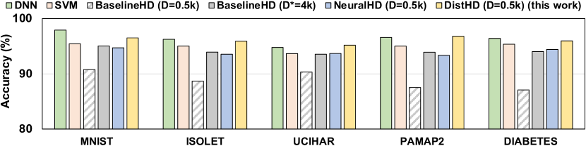
Figure 4: Comparing Classification Accuracy of $\mathsf{DistHD}$ with State-of-the-art Learning Algorithms

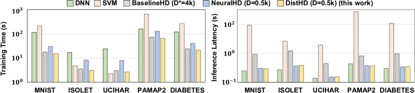
Figure 5: Comparing Training and Inference Efficiency of $\mathsf{DistHD}$ with State-of-the-art Learning Algorithms

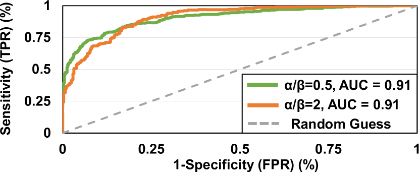
Figure 6: ROC curve of $\mathsf{DistHD}$ using different weight parameters $\alpha$ and $\beta$

IV-A Experimental Setup

We evaluated the effectiveness of our proposed $\mathsf{DistHD}$ learning framework with CPU (Intel Core i9-12900) on widely-used machine learning datasets listed in TABLE I. The $\mathsf{DistHD}$ code was written in Python with NumPy and optimized for performance. We compare $\mathsf{DistHD}$ with state-of-the-art (SOTA) DNNs [27], SVMs [28], SOTA HDC algorithms [21] in terms of accuracy, training and inference efficiency, and robustness against hardware noise. We also compare $\mathsf{DistHD}$ with NeuralHD [7], a recently proposed dynamic encoding technique for HDC aiming at dimension reduction.

IV-B DistHD Accuracy

DistHD vs. SOTA ML Algorithms: We compare the classification accuracy of $\mathsf{DistHD}$ with SOTA learning algorithms, including SOTA deep neural networks (DNNs) and support vector machines (SVMs). The SOTA DNN algorithm is trained with TensorFlow [27] while SVM is trained with the scikit-learn library [28]. We utilize the common practice of grid search to identify the best hyper-parameters for each model. As demonstrated in Fig. 4, $\mathsf{DistHD}$ provides comparable accuracy to SOTA DNNs and 1.17% higher accuracy than SVMs.

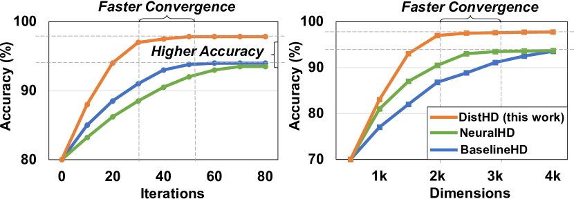
Figure 7: Comparing Convergence Speed of $\mathsf{DistHD}$ with other HDC algorithms

DistHD vs. SOTA HDCs: We compare the accuracy of $\mathsf{DistHD}$ with SOTA HDC algorithms that are incapable of regenerating dimensions (baselineHD) [6] and a recently proposed HDC learning approach using a dynamic encoder (NeuralHD) [7]. The results of baselineHD are reported in two dimensionality: (i) Physical dimensionality ($\mathcal{D}=0.5$k) of NeuralHD and $\mathsf{DistHD}$, a compressed dimensionality designed for resource-constrained computing devices. (ii) Effective dimensionality ($\mathcal{D}^{*}=4\textrm{k}$), defined as the sum of the physical dimensions $(\mathcal{D})$ of $\mathsf{DistHD}$ with the regenerated dimensions throughout the retraining iterations. Mathematically, $\mathcal{D}^{*}=\mathcal{D}+\mathcal{D}\times\mathcal{R}\%\times\textit{Number of Iterations}$, where $\mathcal{R}$ is the regeneration rate. We train each HDC model until it reaches convergence. As shown in Fig. 7, baselineHD and NeuralHD converge at lower accuracy than DistHD due to lacking the capability to fully utilize the information learned during the training process. As demonstrated in Fig. 4, $\mathsf{DistHD}$ ($\mathcal{D}=0.5$k) delivers on average $6.96\%$ and $1.88\%$ higher accuracy than baselineHD ($\mathcal{D}=0.5\textrm{k}$) and NeuralHD ($\mathcal{D}=0.5\textrm{k}$), respectively. Additionally, $\mathsf{DistHD}$ achieves $1.82\%$ higher accuracy than baselineHD ($\mathcal{D}^{*}=4\textrm{k}$). This indicates that $\mathsf{DistHD}$ is capable of outperforming SOTA HDC in terms of accuracy while reducing physical dimensionality by $8.0\times$ on average.

Sensitivity vs. Specificity: We present trade-offs between sensitivity and specificity using ROC curves and area under ROC curves (AUC) in Fig. 6. For two groups of parameters showing comparable accuracy and AUC, with the decrease of the specificity, the model with larger $\alpha$ shows a sharper increase in sensitivity and is more likely to provide higher sensitivity for classification tasks. In contrast, the model with larger $\beta$ loses less specificity with the increase of sensitivity and is more likely to deliver results with higher specificity. We can tune our weight parameters according to the diverse needs of learning tasks for the best outcomes.

IV-C DistHD Efficiency

For fairness, we compare the training and inference efficiency of the SOTA DNN, SVM, baselineHD ($\mathcal{D}^{*}=4\textrm{k}$), NeuralHD ($\mathcal{D}=0.5\textrm{k}$), and $\mathsf{DistHD}$ ($\mathcal{D}=0.5\textrm{k}$) as they achieve comparable accuracy according to Fig. 4. As shown in Fig. 5, SVMs take a significantly longer time for both training and inference for large datasets such as PAMAP and DIABETES. $\mathsf{DistHD}$ delivers considerably higher efficiency than SOTA DNNs ($5.97\times$ faster training, comparable inference latency), SVMs, and SOTA HDC ($1.15\times$ faster training, $8.09\times$ faster inference). $\mathsf{DistHD}$ also delivers a $2.32\times$ speedup in training compared to NeuralHD. $\mathsf{DistHD}$ achieves such high training efficiency due to its capability to reach convergence with noticeably fewer iterations and lower dimensionality than other HDC algorithms, as demonstrated in Fig. 7. Additionally, $\mathsf{DistHD}$ delivers short inference latency since it requires significantly lower dimensionality, effectively accelerating the process of encoding query vectors and calculating similarity scores.

IV-D Robustness of DistHD against Hardware Noises

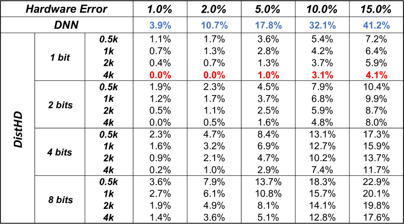
Figure 8: Comparing Quality Loss of $\mathsf{DistHD}$ with DNNs

One of the main advantages of $\mathsf{DistHD}$ is its high robustness against noise and failure. In $\mathsf{DistHD}$, each hypervector stores information across all its components so that no component is more responsible for storing any more information than another, making each hypervector robust against errors. Here we compare the robustness of $\mathsf{DistHD}$ and DNN to hardware noise in Fig. 8 by showing the average quality loss of the DNN and $\mathsf{DistHD}$ under different percentages of hardware errors. The error rate refers to the percentage of random bit flips on memory storing DNN and $\mathsf{DistHD}$ models. For fairness, all DNN weights are quantized to their effective 8-bit representation. In DNN, random bit flip results in significant quality loss as corruptions on most significant bits can cause major weight changes. In contrast, $\mathsf{DistHD}$ provides significantly higher robustness to noise due to its redundant and holographic distribution of patterns in high-dimensional space. Additionally, all dimensions equally contribute to storing information, and thus failure on partial data will not result in the loss of entire information.

$\mathsf{DistHD}$ demonstrates the maximum robustness using hypervectors with $4\textrm{k}$ dimensions in 1-bit precision, that is on average $12.90\times$ higher robustness than DNN. Increasing precision lowers the robustness of $\mathsf{DistHD}$ since random flips on more significant bits will introduce more loss of accuracy. For instance, for $10\%$ bit flips in hardware, $\mathsf{DistHD}$ using 1-bit precision and $4\textrm{k}$ dimensions provides $10.35\times$ and $4.13\times$ higher robustness than DNN and $\mathsf{DistHD}$ using 8 bits with the same dimensionality, respectively. Additionally, higher dimensionality improves the robustness of $\mathsf{DistHD}$ against noise due to more redundant and holographic information distribution. For example, for $10\%$ hardware error, $\mathsf{DistHD}$ using $4\textrm{k}$ dimensions and 8-bit precision achieves $1.43\times$ higher robustness than $\mathsf{DistHD}$ using $0.5\textrm{k}$ dimensions with the same bitwidth.

V Conclusion

In this paper, we propose $\mathsf{DistHD}$, an accurate, efficient, and robust HDC learning framework. With a powerful dynamic encoding technique, $\mathsf{DistHD}$ identifies and regenerates dimensions that mislead the classification and reduce the learning accuracy. Our evaluations on a wide range of machine learning datasets demonstrate that $\mathsf{DistHD}$ delivers on average $2.12\%$ higher accuracy than SOTA HDC algorithms and reduces the dimensionality by $8.0\times$. It also significantly outperforms SOTA DNNs and HDCs in terms of both training and inference efficiency. Additionally, the holographic distribution of patterns in high dimensional space provides $\mathsf{DistHD}$ with $12.90\times$ higher robustness than SOTA DNNs. The performance of $\mathsf{DistHD}$ makes it an outstanding solution for edge platforms.

VI Acknowledgements

This work was supported in part by National Science Foundation #2127780, Semiconductor Research Corporation (SRC), Office of Naval Research, grants #N00014-21-1-2225 and #N00014-22-1-2067, the Air Force Office of Scientific Research under award #FA9550-22-1-0253, and generous gifts from Xilinx and Cisco.

References

• [1] Jiasi Chen and Xukan Ran. Deep learning with edge computing: A review. Proceedings of the IEEE, 2019.
• [2] Weisong Shi et al. Edge computing: Vision and challenges. IEEE Internet of Things journal, 2016.
• [3] Jianli Pan et al. Future edge cloud and edge computing for internet of things applications. Internet of Things Journal, 2017.
• [4] Lulu Ge and Keshab K Parhi. Classification using hyperdimensional computing: A review. IEEE Circuits and Systems Magazine, 2020.
• [5] Mohsen Imani, Yeseong Kim, et al. A framework for collaborative learning in secure high-dimensional space. In CLOUD. IEEE, 2019.
• [6] Abbas Rahimi et al. A robust and energy-efficient classifier using brain-inspired hyperdimensional computing. In ISLPED, 2016.
• [7] Zhuowen Zou et al. Scalable edge-based hyperdimensional learning system with brain-like neural adaptation. In SC, 2021.
• [8] Birgitte Bo Andersen et al. Aging of the human cerebellum: a stereological study. Journal of Comparative Neurology, 2003.
• [9] Pete Warden et al. TinyML. O’Reilly Media, Incorporated, 2019.
• [10] Robert David et al. Tensorflow lite micro: Embedded machine learning for tinyml systems. Proceedings of MLSys, 2021.
• [11] Fouad Sakr, Francesco Bellotti, Riccardo Berta, and Alessandro De Gloria. Machine learning on mainstream microcontrollers. Sensors, 2020.
• [12] X-Cube-AI: AI expansion pack for STM32CubeMX. https://www.st.com/en/embedded-software/x-cube-ai.html.
• [13] Jong Hwan Ko et al. Edge-host partitioning of deep neural networks with feature space encoding for resource-constrained internet-of-things platforms. In AVSS. IEEE, 2018.
• [14] Keith Bonawitz et al. Practical secure aggregation for privacy-preserving machine learning. In ACM SIGSAC CCS, 2017.
• [15] Tian Li et al. Federated learning: Challenges, methods, and future directions. Signal Processing Magazine, 2020.
• [16] Haoyu Luo et al. Keepedge: A knowledge distillation empowered edge intelligence framework for visual assisted positioning in uav delivery. Transactions on Mobile Computing, 2022.
• [17] P. Poduval et al. GrapHD: Graph-based hyperdimensional memorization for brain-like cognitive learning. Frontiers in Neuroscience, 2022.
• [18] Alessio Burrello et al. Laelaps: An energy-efficient seizure detection algorithm from long-term human ieeg recordings without false alarms. In DATE. IEEE, 2019.
• [19] Yeseong Kim et al. Efficient human activity recognition using hyperdimensional computing. In IoT, 2018.
• [20] Mohsen Imani et al. Exploring hyperdimensional associative memory. In HPCA. IEEE, 2017.
• [21] Ali Rahimi and Benjamin Recht. Random features for large-scale kernel machines. Advances in neural information processing systems, 2007.
• [22] Dan Ciregan, Ueli Meier, and Jürgen Schmidhuber. Multi-column deep neural networks for image classification. In CVPR. IEEE, 2012.
• [23] Davide Anguita et al. Human activity recognition on smartphones using a multiclass hardware-friendly support vector machine. In IWAAL. Springer, 2012.
• [24] Hansheng Lei et al. Half-against-half multi-class support vector machines. In International Workshop on Multiple Classifier Systems. Springer, 2005.
• [25] Attila Reiss et al. Introducing a new benchmarked dataset for activity monitoring. In ISWC. IEEE, 2012.
• [26] Beata Strack et al. Impact of hba1c measurement on hospital readmission rates: analysis of 70,000 clinical database patient records. BioMed research international, 2014.
• [27] Hind Taud et al. Multilayer perceptron (mlp). In Geomatic approaches for modeling land change scenarios. Springer, 2018.
• [28] Marti A. Hearst et al. Support vector machines. Intelligent Systems and their applications, 1998.