KGS: Causal Discovery Using Knowledge-guided Greedy Equivalence Search

Abstract

Learning causal relationships solely from observational data provides insufficient information about the underlying causal mechanism and the search space of possible causal graphs. As a result, often the search space can grow exponentially for approaches such as Greedy Equivalence Search (GES) that uses a score-based approach to search the space of equivalence classes of graphs. Prior causal information such as the presence or absence of a causal edge can be leveraged to guide the discovery process towards a more restricted and accurate search space. In this study, we present KGS, a knowledge-guided greedy score-based causal discovery approach that uses observational data and structural priors (causal edges) as constraints to learn the causal graph. KGS is a novel application of knowledge constraints that can leverage any of the following prior edge information between any two variables: the presence of a directed edge, the absence of an edge, and the presence of an undirected edge. We extensively evaluate KGS across multiple settings in both synthetic and benchmark real-world datasets. Our experimental results demonstrate that structural priors of any type and amount are helpful and guide the search process towards an improved performance and early convergence.

1 Introduction

Causal discovery (CD) deals with unfolding the causal relationships among entities in a system. The causes and their corresponding effects are inferred from data, and represented using a causal graph that consists of nodes representing domain variables, and arrows indicating the direction of the relationship between those variables. There exist different approaches to discover the causal structure from data among which the constraint-based (Spirtes et al. [2000], Colombo et al. [2012]) and score-based approaches (Chickering [2002], Chickering and Meek [2015]) are the most prominent ones. Constraint-based approaches perform a series of conditional independence tests to find the causal relationships from data. Whereas, the score-based approaches search over the space of possible graphs to find the graph that best describes the data. Often, these approaches use a search process such as a greedy, A*, or any other heuristic search (Kleinegesse et al. [2022]) combined with a score function such as BIC, AIC, MDL, BDeu, etc. (Meek [2013]) to score all the candidate graphs. The final outcome is one or more causal graphs with the highest score.

Among the score-based approaches, a commonly used approach is the Greedy Equivalence Search (GES) (Chickering [2002]) that searches over the space of equivalence classes of causal graphs. It is an iterative process that starts with an empty network and greedily adds edges one at a time until it reaches the local maximum. Then it continues with a series of greedy deletions of edges until the score keeps improving. Although it is widely used, there are some major disadvantages of this search technique. First, the search space becomes exponential when the number of possible candidate states increases rapidly with the increase in the number of variables (Chickering and Meek [2015], Chickering [2020]). This is because it considers all possible combinations of candidate search states. Hence, a large number of combinations must be considered as the number of variables keep growing, resulting in an exponential growth of the search space (Chickering and Meek [2015]). Even for sparse graphs, the search space is large enough to negatively impact the efficiency and performance of the algorithm. Second, the score needs to be computed for each possible graph which makes it computationally expensive (Chickering and Meek [2015], Chickering [2020]). The situation worsens while traversing the search space of densely-connected models. Because it drastically increases the number of times the algorithm needs to compute the score as it considers almost every node in the respective graph subspace (Chickering [2020]). Furthermore, the search process is typically repeated multiple times, which adds to the overall cost.

To address these challenges in GES, existing causal information can be efficiently used during the discovery process. Often in many domains, there exists some prior information about the causal relationships between some of the variables. This information may be obtained from multiple sources such as domain experts’ opinion, research articles, randomized control trials (RCTs), systematic reviews, and other domain sources. Currently, most of the existing causal discovery approaches are data-driven, rely heavily on the data samples, and do not always consider the available causal knowledge (Kleinegesse et al. [2022]). However, researchers are now getting interested to augment structure learning with known information about causal edges and study their effectiveness to mitigate various practical challenges of causal discovery solely from observational data (Chowdhury et al. [2023]). GES may also be benefited when prior knowledge about some of the causal relationships is used in the form of additional constraints Chickering [2002]. Knowledge constraints may restrict the search space by shifting the focus to a smaller set of potential solutions, thereby, providing a better understanding of the context in which the search is being performed. This may lead towards early convergence resulting in a lower computational cost by reducing the search time, as well as the number of search states that need to be explored. This eventually lowers the number of score calculations too.

To the best of our knowledge, there is no comprehensive study focussing on the application and impact of leveraging the existing causal knowledge in a Greedy score-based causal discovery approach. Therefore, in this work, we present a Knowledge-guided Greedy Equivalence Search (KGS), which leverages knowledge constraints in GES in a systematic way and study how these additional constraints help to guide the search process. We consider three types of causal-edge constraints: (i) Directed edges ($\rightarrow$), (ii) Forbidden edges ($\not\to$), and (iii) Undecided edges (–). These types of prior information about the causal relationships are often available. Here, directed edge and forbidden edge refers to the existence or absence of a causal relationship respectively, and undecided edge refers to the presence of a causal relationship whose direction is unknown. We evaluate the performance of KGS with the three types of edges as well as a combination of all the edges on three synthetic and three benchmark real datasets. We also compare the performances of KGS with GES and present a comparative analysis of how variation in structural prior influences the search process in terms of both graph discovery and computational efficiency. We further study how varying the amount of leveraged knowledge affects the performance of the graph discovery. To summarize, we aim to answer the following questions in this study: 1) How do knowledge constraints affect the learned graph’s accuracy in greedy equivalence search?, 2) Which type of knowledge constraint is the most effective?, 3) How does varying the amount of knowledge influence the performance?, and 4) Do knowledge constraints helps to achieve an early convergence to the optimal causal graph and improves computational efficiency? Our main contributions are summarized below:

• We present KGS, a novel application of causal constraints that leverages available information about different types of edges (directed, forbidden, and undecided) in a Greedy score-based causal discovery approach.

• We demonstrate how the search space as well as scoring candidate graphs can be reduced when different edge constraints are leveraged during a search over equivalence classes of causal networks.

• Through an extensive set of experiments in both synthetic and benchmark real-world settings, we show how different types of prior knowledge can impact the discovery process of graphs of varied densities (small, medium, and large networks).

• We also show the influence of changing the proportion of knowledge constraints on the structure recovery through a set of experiments.

2 Related Works

Conventional CD approaches include Constraint-based approaches that tests for conditional independencies among variables (Spirtes et al. [2000], Spirtes [2001]) and Score-based approaches that scores candidate causal graphs to find the one that best fits the data (Chickering [2002], Chickering and Meek [2015]). Hybrid methods leverage conditional independence tests to learn the skeleton graph and prune a large portion of the search space combined with a score-based search to find the causal DAG (Tsamardinos et al. [2006], Li et al. [2022]). Other common approaches include function-based methods that represent variables as a function of its parents and an independent noise term (Shimizu et al. [2006],Hoyer et al. [2008]). Some recent popular gradient-based approaches use neural networks and a modified definition of the acyclicity constraint (Zheng et al. [2018], Yu et al. [2019], Lachapelle et al. [2019] etc.) that transforms the combinatorial search to a continuous optimization search. These approaches do not consider to leverage any knowledge constraints in the search process. However, multiple studies (Fenton and Neil [2018], Chowdhury et al. [2023]) mention the importance of considering existing causal information when learning causal representation models. Meek [2013] was one of the earliest to suggest orientation rules for incorporating prior knowledge in constraint-based causal discovery approaches. In recent years, there has been an increasing amount of interest in the incorporation of knowledge into causal structure learning (Perković et al. [2017]). Amirkhani et al. [2016] investigated the influence of the same kinds of prior probability on edge inclusion or exclusion from numerous experts which were applied to two variants of the Hill Climbing algorithm. Andrews et al. [2020] incorporates tiered background knowledge in the constraint-based FCI algorithm where they mention that prior knowledge allows for the identification of additional causal links. Fang and He [2020] explores the task of estimating all potential causal effects from observational data using direct and non ancestral causal information. Recently, Hasan and Gani [2022] proposed a generalized framework that uses prior knowledge as constraints to penalize an RL-based search algorithm which outputs the best rewarded causal graph. Kleinegesse et al. [2022] shows that even small amounts of prior knowledge can speed up and improve the performance of A*-based causal discovery. Chowdhury et al. [2023] studies the impact of expert causal knowledge in a continuous optimization-based causal algorithm and suggests that the practitioners should consider utilizing prior knowledge whenever available. Although different approaches have explored the incorporation of prior knowledge in multiple ways, to the best of our knowledge there is no approach that studies the impact and application of different edge constraints in a greedy score-based causal discovery approach.

3 Background

3.1 Causal Graphical Model (CGM)

A directed acyclic graph (DAG) is a type of graph $G$ in which the edges $e$ are directed (→) and there are no cycles. A Causal Graphical Model (CGM) consists of a DAG $G$ and a joint distribution $P$ over a set of random variables $X=(X_{1},X_{2},…,X_{d})$ where $P$ is Markovian with respect to $G$ (Fang and He [2020]). In a CGM, the nodes represent variables X, and the arrows represent causal relationships between them. The joint distribution $P$ can be factorized as follows where $pa(x_{i},G)$ denotes the parents of $x_{i}$ in $G$.

$$P(x_{1},…,x_{d})=\prod_{i=1}^{n}P(x_{i}|pa(x_{i},G)$$ (1)

A set of DAGs having the same conditional independencies belong to the same equivalence class. DAGs can come in a variety of forms based on the kinds of edges they contain. A Partially Directed Graph (PDAG) contains both directed and undirected edges. A Completed PDAG (CPDAG) consists of directed edges that exist in every DAG $G$ belonging to the same equivalence class and undirected edges that are reversible in $G$.

3.2 Score-based Causal Discovery

A score-based causal discovery approach typically searches over the equivalence classes of DAGs to learn the causal graph $G$ that best fits the observed data $D$ as per a score function $S(G,D)$ which returns the score $S$ of $G$ given data $D$ (Chickering [2002], Chowdhury et al. [2023]). Here, the optimization problem for structure learning is as follows:

$$\underset{\text{subject to }G\in D}{\mathop{\min}_{G}}S(G,X)$$ (2)

Typically, any score-based approach has two main components: (i) a search strategy - to traverse the search space of candidate graphs $G$, and (ii) a score function - to evaluate the candidate causal graphs.

Score-function. A scoring function $S(G,D)$ maps causal DAGs $G$ to a numerical score, based on how well $G$ fits to a given dataset $D$. A commonly used scoring function to select causal models is the Bayesian Information Criterion (BIC) (Schwarz [1978]) which is defined below:

$$S_{BIC}=-2*loglikelihood+k*log(n),$$ (3)

where $n$ is the sample size used for training and $k$ is the total number of parameters.

3.3 Greedy Equivalence Search (GES)

GES (Chickering [2002]) is one of the oldest score-based causal discovery methods that employ a greedy search over the space of equivalence classes of DAGs. Each search state is represented by a CPDAG where edge modification operators such as insert and delete operators allow for single-edge additions and deletions respectively. Primarily GES operates in two phases: (i) Forward Equivalence Search (FES) and (ii) Backward Equivalence Search (BES). The first phase FES starts with an empty (i.e., no-edge) CPDAG, and greedily adds edges by considering every single-edge addition that could be performed to every DAG $G$ in the current equivalence class. This phase continues until it reaches a local maximum. After that the second phase BES starts where at each step, it considers all possible single-edge deletions. This continues until there is an improvement of the score. Finally, GES terminates once the second phase reaches a local maximum. GES assumes a decomposable score function $S(G,D)$ which is expressed as a sum of the scores of individual nodes and their parents.

$$S(G,D)=\sum_{i=1}^{d}s(x_{i},pa(x_{i},G))$$ (4)

A problem with GES is that the number of search states that it needs to evaluate scales exponentially with the number of nodes $d$ in the graph (Chickering and Meek [2015]). This results in a vast search space, and also scoring a large number of graphs which adds to the overall cost as score computation is an expensive step.

4 Knowledge-Guided Greedy Equivalence Search

In this section, we introduce our approach Knowledge-guided GES abbreviated as KGS, that uses a set of user-defined knowledge constraints to search for a causal graph that best fits the data and knowledge constraints. The constraints allow KGS to complete the search process using a reduced set of modification operators. KGS primarily works in three steps: (i) knowledge organization, (ii) forward search and (iii) backward search as shown in Algorithm 1 and described in Subsection 4.2.

4.1 Types of Knowledge Constraints

We consider the following types of knowledge constraints (causal edges) between the nodes of a causal graph $G$:
(i) Directed edge (d-edge): The existence of a directed edge (→) from node $X_{i}$ (cause) to node $X_{j}$ (effect). This signifies that these nodes are causally related and $X_{i}$ is the cause of the effect $X_{j}$.
(ii) Forbidden edge (f-edge): The absence of an edge or causal link ($\not\to$) between two nodes $X_{i}$ and $X_{j}$. It signifies the non-existence of a causal relationship between the nodes.
(iii) Undecided edge (u-edge): These are the type of edges whose existence is known, however, their directions are unknown. It signifies the presence of an undirected edge (–) between two nodes $X_{i}$ and $X_{j}$ without any information about the direction of causality.

Assumptions. In this study, we make the following assumptions. First, we assume that there are no hidden variables or selection bias. Second, we assume that the knowledge constraints are 100% true without any bias or error. Third, there can’t be any conflict among the knowledge constraints. That is the same constraint can’t fall into multiple categories. An edge can’t be directed and undecided at the same time.

4.2 Knowledge Incorporation strategy

In this subsection we discuss the steps of KGS in detail.

Step-1: Knowledge Organization. In this step, a knowledge set K is formulated using the available prior causal edges $e_{k}$. The knowledge set is basically a $d\times d$ matrix with entries denoting the prior edges. As per our assumption of bias-free knowledge, only edges that are $100\%$ reliable must be used in this process. Depending on the type of knowledge (directed, forbidden or undecided edge), a $d\times d$ matrix is formed where the entries with ‘1’ indicate a directed edge, ‘2’ for forbidden edge and ‘3’ for undecided edge. Other entries with no information about the edge are denoted by ‘0’. KGS can be used with any one of the three types of knowledge or even with a combination of all of them.

Input: Data $D$, Prior causal edges $E_{k}$.

Output: Causal CPDAG $C$.

Initialize vertex set $V=\{1,...,d\}$ and edge set $E=\emptyset$

Construct knowledge set $K\leftarrow E_{k}$        

$E=E\cup K$

$C$ ($V$, $E$) $\leftarrow$ a CPDAG with $v\in V$ and $e\in E$

$S$ $\leftarrow$ $S_{BIC}(C)$     //Initialize score

    //forward search starts

for each $i$ $\in$ $V$ do

       for each $j$ $\in$ $V$ do

             $I$ $\leftarrow$ $K$-consistent insert operators

            if $i\not\to j\notin K$ then

                  

                  $C^{{}^{\prime}}\leftarrow C\cup(i\rightarrow j)$

                   Compute $S^{{}^{\prime}}\leftarrow S_{BIC}(C^{{}^{\prime}})$

                   if $S^{{}^{\prime}}>S$ then

                         $C\leftarrow C^{{}^{\prime}}$

                         $S$ $\leftarrow$ $S^{{}^{\prime}}$

                   end if

                  

             end if

            

       end for

      

end for

    //backward search starts

for each $i$ $\in$ $V$ do

       for each $j$ $\in$ $V$ do

             $D$ $\leftarrow$ $K$-consistent delete operators

            if $i\rightarrow j$ or $i-j$ $\notin$ $K$ then

                  

                  $C^{{}^{\prime}}\leftarrow C\cup(i\not\to j)$

                  Compute $S^{{}^{\prime}}\leftarrow S_{BIC}(C^{{}^{\prime}})$

                  if $S^{{}^{\prime}}>S$ then

                         $C\leftarrow C^{{}^{\prime}}$

                        $S$ $\leftarrow$ $S^{{}^{\prime}}$

                   end if

                  

             end if

            

       end for

      

end for

return $C$

Algorithm 1 Knowledge-guided GES (KGS)

Step-2: Forward Search. To improve the forward search where edges that provide the current best gain are greedily added, instead of starting with a no-edge model, we start with an initial graph which is a CPDAG that consists of the edges $e_{k}$ present in the knowledge set K. KGS tries to restrict the initial vast set of insert operators based on the directed or undecided edges available in K. This helps in reducing the initial large number of candidate states that were needed to be examined when there is no knowledge constraint. Furthermore, the insert operators that conflict with the forbidden edges in K are completely ignored during the forward search and only $K$-consistent insert operators $I$ are used. This ensures that for any two nodes ($X_{i}$, $X_{j}$) with a $\not\to$ edge in $K$, no unnecessary search is conducted to add an edge between them. This causes the reduction of many search states that might have been explored previously if no knowledge constraints were leveraged. Precisely, it rules out all of the candidate graphs which violate these edges. Going forward in each iteration we choose the candidate graph that gives the highest increment in score, i.e. the graph whose score $S^{{}^{\prime}}$ is better than the current best score $S$, and update the model with the changes done. When there is no further refinement of the score ($S^{{}^{\prime}}$ $<$ $S$), the forward stage stops and the search continues further to the next step.

Step-3: Backward Search. To further refine the graph obtained in the previous phase, we iteratively delete edges and remove the conflicting delete operators to restrict the unnecessary search states. Particularly, the operators that contradict with the directed or undecided edges present in $K$ are ruled out and only $K$-consistent delete operators $D$ are used. Similar to the earlier step, the removal of an edge is allowed only when it improves the score. This process terminates if there is no further improvement in score. Finally, the output is the current graph as the estimated causal DAG.

The time complexity of the Algorithm 1 is $O(n^{2})$ in the worst case since both the loops are nested loops.

4.3 Computational benefits

A potential practical problem GES has is the vast search space that grows exponentially with the increasing number of variables. However, with the use of any available knowledge constraints, this vast growth in the search space can be controlled to a good degree. The forward and backward phases in KGS take into account the user-defined knowledge constraints which influences in shifting the overall search strategy to a more accurate trajectory than GES. Let us consider the case of a 3-node graph in Figure 1. If GES starts with zero knowledge constraints (empty CPDAG), then the space of its DAG equivalence classes consists of a total 25 possible DAGs to choose from. Now, we suppose we are aware of the prior knowledge that a directed edge Y→Z exists for the 3-node graph of Figure 1. Thus, with this prior information, KGS starts with a single-edge model instead of the zero-edge model, and the space of equivalence classes of DAGs are reduced to 8 possible states only. Since we are assuming constraints that are fully accurate, we can prune away the contradictory DAGs, leaving only DAGs that are consistent with the prior knowledge. Thus, it needs to score a much lower number of graphs than earlier due to the guidance of a single edge only. Also, it need not perform expensive score function evaluations for those DAGs that have been pruned away, which may result in significant computational gains. Since in the worst case scenario, the number of search states that GES needs to evaluate can be exponential to the number of nodes (Chickering and Meek [2015]), it is computationally beneficial even if a little amount of knowledge is used to guide or restrict the vast space. Chickering [2002] mentions that enormous savings can be gained by not generating candidates that we are aware of being invalid. Chickering [2002] also suggests that we can prune neighbors heuristically to make the search practical. Leveraging existing knowledge about the causal edges can work as a heuristic because it may help to restrict the search only through equivalence classes where the member DAGs are knowledge consistent.

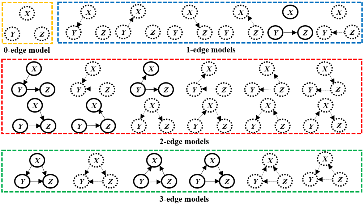
Figure 1: Reduction of the initial search space of a 3-node graph due to leveraging a single causal knowledge (directed edge). Here, the dotted graphs can be ignored based on the prior knowledge $Y\rightarrow Z$ and the bolded graphs are the ones to be considered for initiating the search.

5 Experiments

Table 1: Synthetic dataset results (metric values) averaged over 5 runs with the best results for each dataset boldfaced.

	SHD			TPR			FDR			Run Time (s)
	d-10	d-40	d-100	d-10	d-40	d-100	d-10	d-40	d-100	d-10	d-40	d-100
GES	6	60	107	0.67	0.81	0.84	0.71	0.5	0.41	6.7	2380.7	176552.4
KGS-d	2	30	43	1	0.89	0.95	0.52	0.3	0.2	5.2	1535.9	34417.7
KGS-f	4	52	95	0.8	0.82	0.91	0.6	0.44	0.36	6.1	1312.3	44541.6
KGS-u	2	54	105	1	0.82	0.86	0.5	0.45	0.39	6.3	1833.3	106053.5
KGS-c	2	39	70	1	0.87	0.93	0.51	0.36	0.3	5.3	992.8	39203.8

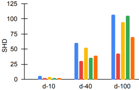
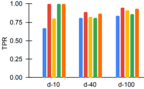
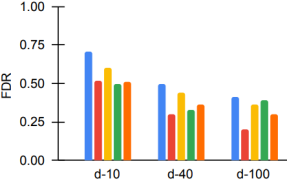
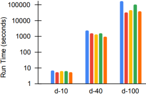
Figure 2: SHD (lower better), TPR (higher better), FDR (lower better) and Run Time (log scale) plots of all the approaches on the synthetic datasets with $d$ = 10, 40, and 100.

We conduct a set of comprehensive experimental evaluations to demonstrate the effectiveness of our proposed approach. We study the impact of directed, forbidden and undecided edges separately as well as the impact of a combination of the three types of edges. We report the performance by comparing the estimated graphs with their ground truths $G_{T}$. We distinguish the experiments with directed, forbidden and undecided edges by naming them as KGS-d, KGS-f and KGS-u respectively. Furthermore, the experiment that uses a combination of all of these edges is named KGS-c. We compare the performance of KGS-d, KGS-f, KGS-u and KGS-c with the baseline approach GES on both synthetic and benchmark real-world datasets. For each experiment, we randomly sample a fixed number (precisely 25%) of edge constraints from the ground-truth network $G_{T}$. As a score function we use a BIC score as it is a standard one as well as the most commonly used score for causal discovery.

Metrics. For performance evaluation, we use three common causal discovery metrics: (i) Structural Hamming Distance (SHD) which denotes the total number of edge additions, deletions and reversals required to transform the estimated graph $G$ to the ground-truth DAG $G_{T}$, (ii) True Positive Rate (TPR) that denotes the ratio of discovered true edges with respect to the total number of edges discovered and (iii) False Discovery Rate (FDR) which denotes the proportion of the estimated false edges. Lower the values of SHD and FDR, and a higher TPR resembles a better causal graph. We also report the run time (in seconds) of each experiment to see if there is any improvement in terms of computational efficiency. The reported metric values are the mean values (averaged over 5 seeds/runs).

Setup. The experiments are conducted on a 4-core Intel Core i5 1.60 GHz CPU cluster, with each process having access to 4 GB RAM. We implemented KGS by extending the publicly available python implementation of GES in the causal-learn package. The source code and experimental datasets are provided as supplementary materials.

Table 2: Real datasets results averaged over 5 seeds with the best performances for each dataset boldfaced.

	SHD			TPR			FDR			Run Time (s)
	Child	Alarm	Hepar2	Child	Alarm	Hepar2	Child	Alarm	Hepar2	Child	Alarm	Hepar2
GES	34	56	70	0.38	0.74	0.5	0.89	0.61	0.23	93.3	762.1	3326.1
KGS-d	25	51	58	0.6	0.84	0.6	0.79	0.57	0.21	40.2	734.3	3225.1
KGS-f	26	48	67	0.62	0.82	0.51	0.79	0.54	0.19	35.1	428.4	1785.6
KGS-u	22	52	59	0.6	0.81	0.57	0.78	0.58	0.2	55.8	747.5	3260.5
KGS-c	23	47	61	0.62	0.79	0.55	0.74	0.55	0.19	33.5	452.4	1774.1

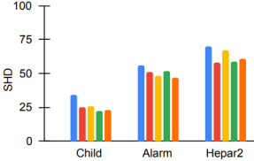
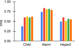
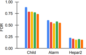
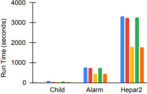
Figure 3: SHD (lower better), TPR (higher better), FDR (lower better) and Run Time (in sec.) plots of all the approaches on the real datasets : Child ($d=20$), Alarm ($d=37$), and Hepar2 ($d=70$).

5.1 Synthetic Data

For synthetic datasets, we employ a similar experimental setup as (Zheng et al. [2018]) and generate random graphs with nodes $d={10,40,100}$ using the Erdős–Rényi (ER) model. The number of nodes are chosen as such to ensure that our approach is tested against networks of all sizes: small, medium and large. Each graph has an edge density of $e$ = 2$d$ where uniform random weights $W$ are assigned to the edges. Data $X$ is generated by taking $n=1000$ i.i.d samples from the linear structural equation model (SEM) $X=W^{T}X+z$, where $z$ is a Gaussian noise term.

Table 1 presents the performance on synthetic datasets (d-10, d-40 and d-100). From Table 1, we can see that clearly knowledge constraints have a positive impact on causal discovery due to the promising metric values. Although the extent of the impact varies for each type of knowledge, it is quite evident from the empirical results that any type of knowledge is beneficial in improving the search quality of GES. In terms of SHD and TPR, KGS-d seems to do better than others for networks of all sizes. This implies that directed edges improve accuracy the most as they provide a more concise or restrained information about the causal relationship than the other constraints. Also, in terms of FDR KGS-d has the best value for two out of three datasets. Overall, it seems that directed edges are more beneficial for producing better graphs with less false positives. KGS-u performs well in terms of all the metrics for the small network only. For networks of larger sizes, it does not perform significantly well. This can be due to the fact that the undecided edges provide partial information as it allows for any one of the two edge possibilities between two random variables $X_{i}$ and $X_{j}$. Either the edge direction can be from $X$ to $Y$ or $Y$ to $X$. The performance of KGS-f suggests that forbidden edges are less effective compared to constraints that provide direct information about the causal edges. This is reasonable as there are relatively more forbidden edges than the directed or undirected edges in a causal graph. The performance of KGS-c is moderately good. In terms of SHD, TPR, and FDR, KGS-c mostly seems to have the second best results which is quite understandable as it has the combined effects of all types of edges. In terms of run time, KGS-d have the fastest speed for the datasets d-10 and d-100. For d-40, KGS-c have the best run time. It seems that as the network density increases, there is a significant difference in the run time of GES and different versions of KGS. For denser graphs (d-40 and d-100), knowledge constraints seems to help a lot in a faster convergence with good margin.

5.2 Real Data

For experimentation with real-world datasets, we evaluate our approach on benchmark causal graphs from the Bayesian Network Repository (BnLearn) (Scutari [2009]). It includes causal graphs inspired by real-world applications that are used as standards in literature. We evaluate GES and all the versions of KGS on 3 different networks namely Child, Alarm and Hepar2 from BnLearn. These networks have available ground-truths and they vary in node and edge densities (small, medium & large networks). The corresponding datasets are available in the causal-learn package. We briefly introduce the networks below:

(i) CHILD (Spiegelhalter et al. [1993]) is a medical Bayesian network for diagnosing congenital heart disease in a new born "blue baby". It is a small network with $d=20$ nodes and $e=25$ edges. The dataset includes patient demographics, physiological features and lab test reports.
(ii) ALARM (Beinlich et al. [1989]) is a healthcare application that sends cautionary alarm messages for patient monitoring. It is used to study probabilistic reasoning techniques in belief networks. The ground-truth graph is a medium sized network with $d=37$ nodes and $e=46$ edges.
(iii) HEPAR2 (Onisko [2003]) is a probabilistic causal model for liver disorder diagnosis. It is a Bayesian network that tries to capture the causal relationships among different risk factors, diseases, symptoms, and test results. It is a large network with $d=70$ nodes and $e=123$ edges.

Table 5 present the results on real datasets. From Table 5 we see that w.r.t SHD, all versions of KGS performs considerably better than GES. KGS-u, KGS-c and KGS-d have the best values of SHD for the Child, Alarm and Hepar2 datasets respectively. Compared to GES, the improvement margin in SHD for all of them is atleast by 10 which is quite impresssive. Overall, none of the SHDs of the estimated graphs by GES is better than KGS. In case of true positives, KGS-d seems to perform really well as it has the best TPR for two out of the three datasets (Alarm and Hepar2). For Child dataset, KGS-f and KGS-c have the highest TPR 0.62 and the TPRs of all the versions of KGS are larger than GES by a good margin. Overall, all versions of KGS have better TPRs than GES for all datasets. For false discoveries, KGS-f and KGS-c performs better than others as both have best FDRs for two out of three real datasets. KGS-c has a 15% improvement in FDR compared to GES for the Child dataset and KGS-f has a 7% lower FDR than GES for Alarm dataset. For Hepar2, the improvement margin is low (4%) which is still significant. In terms of run time, KGS-c is mostly faster than others with the lowest run time for two datasets (Child and Hepar2). For the other dataset Alarm, KGS-f is the fastest. One thing is common w.r.t. run time for all the 3 real datasets. The run time for KGS-f and KGS-c is quite close in all of these datasets. It signifies that forbidden edges may allow the search process to converge faster. Although forbidden edge constraints are not the best among all the edge constraints in terms of the accuracy metrics, they seem to perform well w.r.t faster convergence.

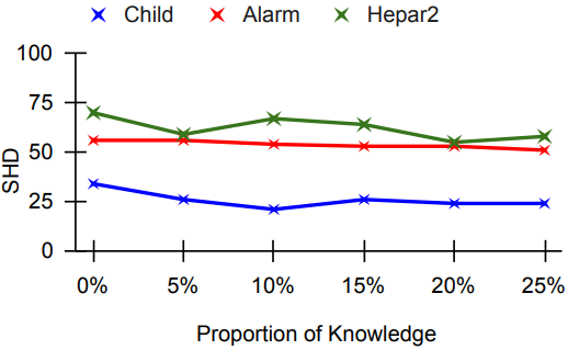
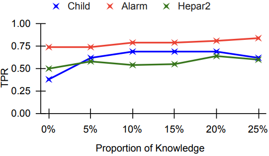
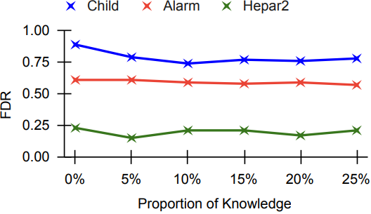
Figure 4: Variation in SHD (lower better), TPR (higher better), and FDR (lower better) due to changing the proportion of knowledge constraints.

5.3 Variation of Knowledge Proportion

We perform an experiment by leveraging different amount of prior edges to investigate two aspects: (i) Do raising the amount of knowledge improves the discovery? and (ii) How varying the amount of knowledge affects the structure search. This experiment is done on the real datasets by varying the amount of directed edges from 0 to 25 percent. Each time the amount of prior knowledge is raised by 5%. From the plots in Figure 4, we see that using any amount of prior knowledge is always better than using no knowledge at all (0 percent). This is because all of the metrics SHD, TPR and FDR have better values for the experiments where at least some knowledge is used. Although in some cases the improvement can be very less or same (TPR of the experiments 0 % and 5 % for Alarm), in no cases there is a negative impact of using knowledge. Another finding from the plots is that increasing the amount of knowledge is not always proportional to better metric values. The drop in SHD and FDR, and also, the rise in TPR due to the changing % of knowledge is quite unsteady. However, it seems like leveraging any amount of causal knowledge is always better than leveraging no knowledge at all.

Table 3: Correction ($C$) of edges after graph estimation.

Data	Method	$K$	TP	TP$\in$$K$	$C$	TP after $C$ (TPC)	FP	FN
d-10	GES	–	4	2	3	4+3 = 7	10	2
	KGS-d	5	6	3	2	6+2 = 8	5	0
Child	GES	–	5	2	4	5+4 = 9	39	8
	KGS-d	6	8	4	2	8+2 = 10	28	5

5.4 Manual Correction of Edges

We perform a sanity check to ensure if graphs discovered by KGS are better than those of GES even after manual correction of the estimated edges belonging to the knowledge set $K$. As part of our sanity check, we investigate the number of edges required to be corrected in the graphs produced by GES and KGS. A lower number of corrections to be done and a higher number of true positives signifies a better performance. We perform this check for the directed edges experiment (KGS-d) on one synthetic (d-10) and one real dataset (Child). From Table 3, we see that for d-10 and Child, the set of prior directed edges for KGS-d contains $K$ = 5 and $K$ = 6 edges respectively and GES uses no prior knowledge constraints. With this experimental setting, GES discovers less true positive edges (column TP) than KGS-d. The column TP $\in K$ denotes the number of discovered TP edges that are also element of $K$. Thus, the no. of manual corrections is $C$ = $K$ - (TP $\in$ $K$). Here, we see that GES requires more edge corrections ($C$) than KGS-d. As a result, the total TPs after manual corrections (TP_C) are higher for KGS-d than GES. This is the case for small networks. For medium to larger networks this difference in TPs can be higher. In terms of false positives (FP), KGS-d performs quite better than GES as their is a significant reduction in the number of estimated FP edges. Also, the false negatives (FN) are lower in KGS-d than GES for both the datasets. To summarize, guidance from prior knowledge is significant for conducting an efficient search w.r.t. true and false discoveries as well as estimating a more accurate graph than the one produced by GES without any knowledge guidance.

6 Conclusion

In this study, we introduce KGS, which presents a novel application of prior edge constraints in a score-based causal search process. We evaluate KGS’s performance on a variety of synthetic and real-world datasets, including networks of different sizes and edge densities. The encouraging results across multiple settings demonstrate the robustness and flexibility of our approach. Particularly, KGS-d, that leverages directed edges performs the best in most cases for improving the graphical accuracy as well as for faster convergence. This is quite understandable as directed edges provide a complete information about the causal relation between variables. Overall, any type of edge information improves the accuracy of the graph discovery as well as the run time compared to the performance of GES which uses no knowledge. Hence, it is evident that prior knowledge is helpful for guiding the search to a better trajectory. There are some limitations of this study. First, in this study, we consider only those causal knowledge that is completely true. That is any biased knowledge is out of the scope of this work. Second, this approach has a limited application when there is no prior knowledge available. Although it is often the case that at least some prior knowledge about any domain is available. In future, we want to extend this study to address biases in prior knowledge and also, study the effects of localizing the knowledge to a sub-area of the network and see how it impacts the discovery in other areas.

APPENDIX

Appendix A Additional simulation results

We present the total number of estimated models by the different versions of KGS and GES for both synthetic and real datasets in Table 4. The total estimated models signify the number of models or graphs that were required to be estimated by the algorithm before reaching convergence (final best scored causal graph). A lower number of this metric signifies a better performance by the approach, and also a lower number of calls to the scoring function.

Table 4: Total estimated models before convergence with best results boldfaced for each of the datasets.

Estimated Models (lower better)
Methods	d-10	d-40	d-100	Child	Alarm	Hepar2
GES	20	152	333	49	84	83
KGS-d	15	101	220	34	74	66
KGS-f	19	131	300	40	81	80
KGS-u	16	135	313	33	74	73
KGS-c	16	100	290	34	70	66

A.1 EXPERIMENTAL RESULTS of Varying the knowledge proportion

We present the details of all the metric values for the experiment done with varying the amount of prior knowledge in Table 5. This experiment is done by varying the amount of constraints (directed edges) from 0 to 25 percent each time by raising the amount of knowledge by 5%. The results show that any amount of knowledge is good for improving search accuracy and hence should be leveraged during the search process. Although it is surprising that the increment in knowledge is not directly proportional to the increment in discovery accuracy. Still leveraging any percentage of knowledge is better than using no knowledge at all.

Table 5: Results (metric values) of the experiment done by varying the knowledge proportion.

Datasets	Proportion of Knowledge	SHD (lower better)	TPR (higher better)	FDR (lower better)	Estimated models (lower better)
Child	0%	34	0.38	0.89	49
	5%	26	0.62	0.79	39
	10%	21	0.69	0.74	36
	15%	26	0.69	0.77	37
	20%	24	0.69	0.76	35
	25%	24	0.62	0.78	34
Alarm	0%	56	0.74	0.61	84
	5%	56	0.74	0.61	82
	10%	54	0.79	0.59	83
	15%	53	0.79	0.58	76
	20%	53	0.81	0.59	77
	25%	51	0.84	0.57	74
Hepar2	0%	70	0.5	0.23	83
	5%	59	0.58	0.15	81
	10%	67	0.54	0.21	76
	15%	64	0.55	0.21	73
	20%	55	0.64	0.17	71
	25%	58	0.6	0.21	66

A.2 Performance of baseline causal discovery approaches

We report the performance of different baseline causal discovery approaches such as PC (constraint-based), LiNGAM (FCM-based) and NOTEARS (continuous optimization-based) on the synthetic and real datasets to see their comparative performance with respect to GES and KGS. We briefly discuss the methods below:

(i) PC algorithm: The Peter-Clark (PC) algorithm (Spirtes et al. [2000]) is a very common constraint-based causal discovery approach that largely depends on conditional independence (CI) tests to find the underlying causal graph. Primarily, it works in three steps: (i) Skeleton construction, (ii) V-structures determination, and (iii) Edge orientations.

(ii) LiNGAM: Linear Non-Gaussian Acyclic Model (LiNGAM) uses a statistical method known as independent component analysis (ICA) to discover the causal structure from observational data. It makes some strong assumptions such as the data generating process is linear, there are no unobserved confounders, and noises have non-Gaussian distributions with non-zero variances (Shimizu et al. [2006]). DirectLiNGAM (dLiNGAM) is an efficient variant of the LiNGAM approach that uses a direct method for learning a linear non-Gaussian structural equation model (Shimizu et al. [2011]). The direct method estimates causal ordering and connection strengths based on non-Gaussianity.

(iii) NOTEARS: DAGs with NO TEARS (Zheng et al. [2018]) is a recently developed causal discovery algorithm that reformulates the structure learning problem as a purely continuous constrained optimization task. It uses an algebraic characterization of DAGs and defines a novel characterization of acyclicity that allows for a smooth global search, instead to a combinatorial search.

For experimental purpose, the implementations of the algorithms have been adopted from the gCastle (Zhang et al. [2021] repository. From the results reported in Table 6, we see that in few cases NOTEARS performs slightly better than KGS particularly for SHD and FDR metrics. However, it performs poorly in terms of discovering the true edges (TPR). Also, it could not even estimate a single graph for the case of Hepar2 dataset. The dLiNGAM approach performs better than KGS only twice, once w.r.t. SHD and once w.r.t FDR. Otherwise its performance is mostly moderate. PC does not perform well in case of any of the metrics at all. The boldfaced results in the table are the ones that are better than that of KGS for the corresponding datasets.

Table 6: Performance metrics of the baseline approaches on the synthetic and real datasets.

	d-10			d-40			d-100			Child			Alarm			Hepar2
Method	SHD	TPR	FDR	SHD	TPR	FDR	SHD	TPR	FDR	SHD	TPR	FDR	SHD	TPR	FDR	SHD	TPR	FDR
PC	13	0.42	0.47	74	0.5	0.49	187	0.47	0.5	43	0.24	0.86	55	0.67	0.6	172	0.35	0.75
dLiNGAM	18	0.37	0.53	169	0.4	0.79	246	0.6	0.6	28	0.12	0.82	40	0.39	0.5	110	0.1	0.07
NOTEARS	3	0.8	0.1	78	0.6	0.49	472	0.66	0.75	22	0.16	0.63	41	0.17	0.38	123	-	-

Appendix B Performance metrics details

• Structural Hamming Distance (SHD): SHD is the sum of the edge additions (A), deletions (D) or reversals (R) that are required to convert the estimated graph into the true causal graph (Zheng et al. [2018], Cheng et al. [2022]). To estimate SHD it is required to determine the missing edges, extra edges and edges with wrong direction in the estimated graph compared to the true graph. Lower the SHD closer is the graph to the true graph and vice versa. The formula to calculate SHD is given below:

$$SHD=A+D+R$$ (5)

• True Positive Rate (TPR): TPR denotes the proportion of the true edges in the actual graph that are correctly identified as true in the estimated graph. A higher value of the TPR metric means a better causal discovery.

$$TPR=\frac{TP}{TP+FN}$$ (6)

Here, TP means the true positives or the number of correctly identified edges and FN or false negatives denote the number of unidentified causal edges.

• False Discovery Rate (FDR): FDR is the ratio of false discoveries among all discoveries (Zheng et al. [2018]). FDR represents the fraction of the false edges over the sum of the true and false edges. Lower the FDR, better is the outcome of causal discovery.

$$FDR=\frac{FP}{TP+FP}$$ (7)

Here, FP or false positives represent the number of wrongly identified directed edges.

Appendix C Code and Data

The code for reproducing KGS and the datasets used in this study are publicly available in the following GitHub link: https://github.com/UzmaHasan/KGS-Causal-Discovery-Using-Constraints.

References

- Amirkhani et al. [2016] Hossein Amirkhani, Mohammad Rahmati, Peter JF Lucas, and Arjen Hommersom. Exploiting experts’ knowledge for structure learning of bayesian networks. IEEE transactions on pattern analysis and machine intelligence, 39(11):2154–2170, 2016.
- Andrews et al. [2020] Bryan Andrews, Peter Spirtes, and Gregory F Cooper. On the completeness of causal discovery in the presence of latent confounding with tiered background knowledge. In International Conference on Artificial Intelligence and Statistics, pages 4002–4011. PMLR, 2020.
- Beinlich et al. [1989] Ingo A Beinlich, Henri Jacques Suermondt, R Martin Chavez, and Gregory F Cooper. The alarm monitoring system: A case study with two probabilistic inference techniques for belief networks. In AIME 89, pages 247–256. Springer, 1989.
- Cheng et al. [2022] Lu Cheng, Ruocheng Guo, Raha Moraffah, Paras Sheth, Kasim Selcuk Candan, and Huan Liu. Evaluation methods and measures for causal learning algorithms. IEEE Transactions on Artificial Intelligence, 2022.
- Chickering [2002] David Maxwell Chickering. Optimal structure identification with greedy search. Journal of machine learning research, 3(Nov):507–554, 2002.
- Chickering and Meek [2015] David Maxwell Chickering and Christopher Meek. Selective greedy equivalence search: Finding optimal bayesian networks using a polynomial number of score evaluations. arXiv preprint arXiv:1506.02113, 2015.
- Chickering [2020] Max Chickering. Statistically efficient greedy equivalence search. In Conference on Uncertainty in Artificial Intelligence, pages 241–249. PMLR, 2020.
- Chowdhury et al. [2023] Jawad Chowdhury, Rezaur Rashid, and Gabriel Terejanu. Evaluation of induced expert knowledge in causal structure learning by notears. arXiv preprint arXiv:2301.01817, 2023.
- Colombo et al. [2012] Diego Colombo, Marloes H Maathuis, Markus Kalisch, and Thomas S Richardson. Learning high-dimensional directed acyclic graphs with latent and selection variables. The Annals of Statistics, pages 294–321, 2012.
- Fang and He [2020] Zhuangyan Fang and Yangbo He. Ida with background knowledge. In Conference on Uncertainty in Artificial Intelligence, pages 270–279. PMLR, 2020.
- Fenton and Neil [2018] Norman Fenton and Martin Neil. Risk assessment and decision analysis with Bayesian networks. Crc Press, 2018.
- Hasan and Gani [2022] Uzma Hasan and Md Osman Gani. Kcrl: A prior knowledge based causal discovery framework with reinforcement learning. Proceedings of Machine Learning Research, 182(2022):1–24, 2022.
- Hoyer et al. [2008] Patrik Hoyer, Dominik Janzing, Joris M Mooij, Jonas Peters, and Bernhard Schölkopf. Nonlinear causal discovery with additive noise models. Advances in neural information processing systems, 21, 2008.
- Kleinegesse et al. [2022] Steven Kleinegesse, Andrew R Lawrence, and Hana Chockler. Domain knowledge in a*-based causal discovery. arXiv preprint arXiv:2208.08247, 2022.
- Lachapelle et al. [2019] Sébastien Lachapelle, Philippe Brouillard, Tristan Deleu, and Simon Lacoste-Julien. Gradient-based neural dag learning. arXiv preprint arXiv:1906.02226, 2019.
- Li et al. [2022] Yan Li, Rui Xia, Chunchen Liu, and Liang Sun. A hybrid causal structure learning algorithm for mixed-type data. 2022.
- Meek [2013] Christopher Meek. Causal inference and causal explanation with background knowledge. arXiv preprint arXiv:1302.4972, 2013.
- Onisko [2003] Agnieszka Onisko. Probabilistic causal models in medicine: Application to diagnosis of liver disorders. In Ph. D. dissertation, Inst. Biocybern. Biomed. Eng., Polish Academy Sci., Warsaw, Poland, 2003.
- Perković et al. [2017] Emilija Perković, Markus Kalisch, and Maloes H Maathuis. Interpreting and using cpdags with background knowledge. arXiv preprint arXiv:1707.02171, 2017.
- Schwarz [1978] Gideon Schwarz. Estimating the dimension of a model. The annals of statistics, pages 461–464, 1978.
- Scutari [2009] Marco Scutari. Learning bayesian networks with the bnlearn r package. arXiv preprint arXiv:0908.3817, 2009.
- Shimizu et al. [2006] Shohei Shimizu, Patrik O Hoyer, Aapo Hyvärinen, Antti Kerminen, and Michael Jordan. A linear non-gaussian acyclic model for causal discovery. Journal of Machine Learning Research, 7(10), 2006.
- Shimizu et al. [2011] Shohei Shimizu, Takanori Inazumi, Yasuhiro Sogawa, Aapo Hyvärinen, Yoshinobu Kawahara, Takashi Washio, Patrik O Hoyer, and Kenneth Bollen. Directlingam: A direct method for learning a linear non-gaussian structural equation model. The Journal of Machine Learning Research, 12:1225–1248, 2011.
- Spiegelhalter et al. [1993] David J Spiegelhalter, A Philip Dawid, Steffen L Lauritzen, and Robert G Cowell. Bayesian analysis in expert systems. Statistical science, pages 219–247, 1993.
- Spirtes [2001] Peter Spirtes. An anytime algorithm for causal inference. In International Workshop on Artificial Intelligence and Statistics, pages 278–285. PMLR, 2001.
- Spirtes et al. [2000] Peter Spirtes, Clark N Glymour, Richard Scheines, and David Heckerman. Causation, prediction, and search. MIT press, 2000.
- Tsamardinos et al. [2006] Ioannis Tsamardinos, Laura E Brown, and Constantin F Aliferis. The max-min hill-climbing bayesian network structure learning algorithm. Machine learning, 65(1):31–78, 2006.
- Yu et al. [2019] Yue Yu, Jie Chen, Tian Gao, and Mo Yu. Dag-gnn: Dag structure learning with graph neural networks. In International Conference on Machine Learning, pages 7154–7163. PMLR, 2019.
- Zhang et al. [2021] Keli Zhang, Shengyu Zhu, Marcus Kalander, Ignavier Ng, Junjian Ye, Zhitang Chen, and Lujia Pan. gcastle: A python toolbox for causal discovery. arXiv preprint arXiv:2111.15155, 2021.
- Zheng et al. [2018] Xun Zheng, Bryon Aragam, Pradeep K Ravikumar, and Eric P Xing. Dags with no tears: Continuous optimization for structure learning. Advances in Neural Information Processing Systems, 31, 2018.