Spatio-temporal fluctuations of interscale and interspace energy transfer dynamics in homogeneous turbulence

Abstract

We study fluctuations of all co-existing energy exchange/transfer/transport processes in stationary periodic turbulence including those which average to zero and are not present in average cascade theories. We use a Helmholtz decomposition of accelerations which leads to a decomposition of all terms in the Kármán-Howarth-Monin-Hill (KHMH) equation (scale-by-scale two-point energy balance) causing it to break into two energy balances, one resulting from the integrated two-point vorticity equation and the other from the integrated two-point pressure equation. The various two-point acceleration terms in the Navier-Stokes difference (NSD) equation for the dynamics of two-point velocity differences have similar alignment tendencies with the two-point velocity difference, implying similar characteristics for the NSD and KHMH equations. We introduce the two-point sweeping concept and show how it articulates with the fluctuating interscale energy transfer as the solenoidal part of the interscale transfer rate does not fluctuate with turbulence dissipation at any scale above the Taylor length but with the sum of the time-derivative and the solenoidal interspace transport rate terms. The pressure fluctuations play an important role in the interscale and interspace turbulence transfer/transport dynamics as the irrotational part of the interscale transfer rate is equal to the irrotational part of the interspace transfer rate and is balanced by two-point fluctuating pressure work. We also study the homogeneous/inhomogeneous decomposition of interscale transfer. The statistics of the latter are skewed towards forward cascade events whereas the statistics of the former are not. We also report statistics conditioned on intense forward/backward interscale transfer events.

1 Introduction

Modeling of turbulence dissipation is a cornerstone of one-point turbulent flow prediction methods based on the Reynolds Averaged Navier Stokes (RANS) equations such as the widely used $k-\varepsilon$ and the $k-\omega$ models (see Pope (2000), Leschziner (2016)) and also of two-point turbulence flow prediction methods based on filtered Navier Stokes equations, namely Large Eddy Simulations (LES) (see Pope (2000), Sagaut (2000)). The mechanism of turbulence dissipation away from walls is the turbulence cascade (Pope, 2000; Vassilicos, 2015). Indeed, without cascade, the larger turbulent eddies which constitute the most energetic part of the turbulence, would take much longer to lose their energy than just one or a few eddy turnover times. The physical understanding of this cascade which, to this day, has underpinned these prediction methods is based on Kolmogorov’s average cascade in statistically homogeneous and stationary turbulence. Notwithstanding recent advances which have shown that the turbulence dissipation and cascade are different from Kolmogorov’s both in non-stationary (see e.g. Vassilicos (2015); Goto & Vassilicos (2016); Steiros (2022)) and in non-homogeneous turbulence (Chen et al., 2021; Chen & Vassilicos, 2022), Kolmogorov’s cascade is in fact valid only as an average cascade even in homogeneous stationary turbulence. Turbulence has been known to be intermittent since the late 1940s (see Frisch (1995) and references therein), and this intermittency has mainly been taken into account as structure function exponent corrections to Kolmogorov’s average picture. However, Yasuda & Vassilicos (2018) studied intermittent fluctuations without reference to structure function exponents which require high Reynolds numbers to be well defined and to be predicted from Kolmogorov’s theory or various intermittency-accounting variants of this theory (see Frisch (1995) and references therein). They concentrated their attention on the actual fundamental basis of Kolmogorov’s theory which is scale-by-scale equilibrium for statistically homogeneous and stationary turbulence, and not on the theory’s structure function and energy spectrum scaling consequences. The scale-by-scale equilibrium implied by statistical homogeneity and stationarity is that the average interscale turbulence energy transfer rate is balanced by nothing more than average scale-by-scale viscous diffusion rate, average turbulence dissipation rate and average energy input rate by a stirring force, irrespective of Reynolds number (except that the Reynolds number needs to be large enough for the presence of random fluctuations). It is most natural for a study of intermittency to start with the fluctuations around this balance, which means that along with the fluctuations of interscale transfer, dissipation, diffusion and energy input, all other fluctuating turbulent energy change rates need to be taken into account as well even if their spatio-temporal average is zero in statistically stationary homogeneous turbulence. The intermittency corrections to Kolmogorov’s average cascade theory which have been developed since the 1960s (e.g. see Frisch (1995); Sreenivasan & Antonia (1997)) are often based on the intermittent fluctuations of the local (in space and time) turbulence dissipation rate, yet Yasuda & Vassilicos (2018) demonstrated that these dissipation fluctuations are much less intense than the fluctuations of other turbulent energy change rates such as the non-linear interspace energy transfer rate (which is a scale-by-scale rate of turbulent transport in physical space), the fluctuating work resulting from the correlation of the fluctuating pressure gradient with the fluctuating velocity and the time-derivative of the scale-by-scale turbulent kinetic energy. Yasuda & Vassilicos (2018) made these observations using Direct Numerical Simulations (DNS) of statistically stationary periodic turbulence at low to moderate Taylor length-based Reynolds numbers from about 80 to 170. Even though their Reynolds numbers were not high enough to test the high Reynolds number scaling consequences of Kolmogorov’s theory, they observed an energy spectrum with a near-decade power law range where the power law exponent was not too far from Kolmogorov’s $-5/3$. However, they did not observe a significant range of scales where the scale-by-scale equilibrium reduces to a scale-by-scale balance between average interscale turbulence energy transfer rate and average turbulence dissipation as predicted by the Kolmogorov theory for statistically stationary homogeneous turbulence at asymptotically high Reynolds numbers. This high Reynolds number scale-by-scale equilibrium is the trademark of the Kolmgorov average cascade and is typically not put in question by existing intermittency corrections to Kolmogorov’s theory (e.g. see Frisch (1995)).

Given the low to moderate Reynolds numbers of the DNS used by Yasuda & Vassilicos (2018), their observations concern interscale turbulence energy transfers more than the turbulence cascade per se if the concept of turbulence cascade is taken to have meaning only at very large Reynolds numbers. They demonstrated that an interscale transfer picture appears that is radically different from Kolmogorov’s if the average is lifted and all spatio-temporal intermittent fluctuations are taken into account. This different picture involves highly fluctuating processes which vanish on average in statistically stationary and homogeneous turbulence and are not taken into account by the Kolmogorov theory for that very reason. We stress once more that Yasuda & Vassilicos (2018) made this demonstration in statistically homogeneous and stationary turbulence, the very type of turbulence where Kolmogorov’s theory has been designed for.

It is hard to imagine that the complex turbulence energy transfer picture educed by the DNS of Yasuda & Vassilicos (2018) does not survive at asympotically high Reynolds numbers because it is known that the small-scale turbulence becomes increasingly intermittent with increasing Reynolds number (e.g. see Frisch (1995); Sreenivasan & Antonia (1997)). A DNS study at higher Reynolds numbers is nevertheless needed to ascertain this point. However, this is not the study proposed in this paper. In this paper our aim is to gain deeper insight into the fluctuating energy transfer picture revealed by the DNS of Yasuda & Vassilicos (2018) and we do this in terms of Helmholtz decomposed solenoidal and irrotational acceleration fields. Given that the computational cost involved in this Helmholtz decomposition is high (see following two sections) it is not possible for us to carry out our study for a variety of increasing Reynolds numbers and thereby combine it with a Reynolds number dependence study. We therefore limit ourselves to Reynolds numbers comparable to those of Yasuda & Vassilicos (2018).

The radically different turbulence energy transfer picture which appears when all intermittent turbulence fluctuations are taken into account exhibits correlations between fluctuations of different processes: in particular, the fluctuating pressure-velocity term mentioned above is correlated with the interscale energy transfer rate, and the time derivative of the turbulent kinetic energy below a certain two-point length $r$ is correlated with the inter-space energy transport rate at the same length $r$. Yasuda & Vassilicos (2018) explained the former correlation as resulting from the link between non-linearity and non-locality (via the pressure field) and the latter correlation as reflecting the passive sweeping of small turbulent eddies by large ones (Tennekes, 1975). However, this sweeping (also termed “random Taylor hypothesis”) has been studied by reference to the one-point incompressible Navier-Stokes equation (e.g. Tennekes (1975), Tsinober et al. (2001)) rather than the two-point Kármán-Howarth-Monin-Hill (KHMH) equation, used by Yasuda & Vassilicos (2018) in their study of the fluctuating turbulence cascade. The KHMH equation is a scale-by-scale energy budget local in space and time, directly derived from the incompressible Navier-Stokes equations for the instantaneous velocity field (see Hill (2002)) without decomposition (e.g. Reynolds decomposition), without averages (e.g. Reynolds averages), and without any assumption made about the turbulent flow (e.g. homogeneity, isotropy, etc.). The initial trigger of the present paper is to substantiate the claim of Yasuda & Vassilicos (2018) concerning correlations being caused by random sweeping by translating the sweeping analysis of Tsinober et al. (2001) to the KHMH equation. It is in doing so that we espouse the Helmholtz decomposition which Tsinober et al. (2001) introduced for the analysis of the acceleration field. We apply it to the two-point Navier-Stokes difference (NSD) equation (which is the equation governing the dynamics of two-point velocity differences) and the KHMH equation which derives from it. This decomposition into solenoidal and irrotational terms breaks the Navier-Stokes equation into two equations, one being the irrotational balance between non-linearity and non-locality (pressure) and the other being the solenoidal balance between local unsteadiness and advection which encapsulates the sweeping. With this decomposition we substantiate all the correlations observed by Yasuda & Vassilicos (2018) between different KHMH terms representing different energy change processes, not only the ones caused by sweeping. In fact, we educe the relation between interspace turbulence energy transfer/transport and two-point sweeping (i.e. the random Taylor hypothesis that we generalise to two-point statistics), and we extend the correlation study to solenoidal and irrotational sub-terms of the KHMH equation which leads to even stronger correlations than those found by Yasuda & Vassilicos (2018). This approach sheds some light on the way that two-point sweeping and interscale energy transfer relate to each other. We then ask whether the scale-by-scale equilibrium which is at the basis of Kolmogorov’s theory and which disappears when the average is lifted does nevertheless exist locally at relatively high energy transfer events, a question which leads us to consider whether two-point sweeping also holds at such events. Finally, we study the recently introduced decomposition (Alves Portela et al., 2020) of the interscale transfer rate into a homogeneous and an inhomogeneous interscale transfer component. We analyse their fluctuations and the correlations of these fluctuations, both unconditionally and conditionally on relatively rare intense interscale transfer events.

In the following section we introduce our direct numerical simulations (DNSs) of forced periodic turbulence. Subsection 3.1 is a reminder of the application of this decomposition to the one-point Navier-Stokes equation by Tsinober et al. (2001). In this sub-section we also validate our DNS by retrieving the conclusions of Tsinober et al. (2001) on sweeping and by comparing our DNS results on one-point acceleration dynamics to theirs. In subsections 3.2-3.3 we apply the Helmholtz decomposition to the two-point NSD equation for the case of homogeneous/periodic turbulence and in subsection 3.4 we derive from the Helmholtz decomposed Navier-Stokes difference equations corresponding KHMH equations. Subsection 3.4 formalises the connection between the NS and KHMH dynamics, clarifies under which conditions a link exists between NS and KHMH dynamics and provides results on scale and Reynolds number dependencies of the KHMH dynamics. By considering the NSD dynamics in terms of solenoidal and irrotational dynamics, we derive two new KHMH equations. In section 4 we use these two new KHMH equations to obtain new results on the fluctuating cascade dynamics across scales both unconditionally and conditionally on rare extreme interscale energy transfer events. In section 5 we analyse the inhomogeneous and homogeneous contributions to the interscale energy transfer rate. Finally, section 6 summarises our results.

2 DNS of body-forced period turbulence

$N$	$\langle\Rey_{\lambda}\rangle_{t}$	$\nu/10^{3}$	$k_{\text{max}}\langle\eta\rangle_{t}$	$2\upi/\langle L\rangle_{t}$	$\langle\lambda\rangle/\langle L\rangle_{t}$	$T_{s}/T$	$\Delta T/T$
256	112	1.80	1.88	5.6	3.5	21	0.01
512	174	0.72	1.89	5.4	5.2	27	0.12

Table 1: Specifications of the numerial simulations. $N$ denotes the number of grid points in each Cartesian coordinate, $Re_{\lambda}$ the Taylor-scale Reynolds number, $\nu$ the kinematic viscosity, $k_{\text{max}}=\sqrt{2}/3N$ is the highest resolved wavenumber, $\eta$ and $\lambda$ are, respectively, the Kolmogorov and Taylor lengths and $\langle\ldots\rangle_{t}$ denotes a time-average. $L$ is the integral lengths calculated from the three-dimensional energy spectrum $E(k,t)$: $L(t)=(3\pi/4)\int_{0}^{\infty}k^{-1}E(k,t)dk/K(t)$ where $K(t)$ is the kinetic energy per unit mass. $T_{s}$ denotes the total sampling time over which converged statistics are calculated by sampling randomly in space-time, $\Delta T$ denotes the time between samples and $T\equiv\langle L\rangle_{t}/\sqrt{2/3\langle K\rangle_{t}}$ is the turnover time.

Our study requires turbulence data from a turbulent flow where the Kolmogorov equilibrium theory for statistically homogeneous and stationary turbulence is applicable. We therefore follow Yasuda & Vassilicos (2018) and perform Direct Numerical Simulations of body-forced periodic Navier-Stokes turbulence with the same pseudo-spectral code that they used. This code solves numerically the vorticity equation

$$\frac{\partial\boldsymbol{\omega}}{\partial t}=\nabla_{\boldsymbol{x}}\times(\boldsymbol{u}\times\boldsymbol{\omega})+\nu\nabla_{\boldsymbol{x}}^{2}\boldsymbol{\omega}+\nabla_{\boldsymbol{x}}\times\boldsymbol{f},$$ (1)

subjected to the continuity equation

$$\nabla_{\boldsymbol{x}}\cdot\boldsymbol{u}=0,$$ (2)

where $\boldsymbol{u}(\boldsymbol{x},t)$, $\boldsymbol{f}(\boldsymbol{x},t)$ and $\boldsymbol{\omega}(\boldsymbol{x},t)$ are the velocity, force and vorticity fields respectively and $\nu$ is the kinematic viscosity. All fields are $2\pi$-periodic in each one of the three orthogonal spatial coordinates $x_{1}$, $x_{2}$ and $x_{3}$, and $\boldsymbol{x}=(x_{1},x_{2},x_{3})$. The pseudo-spectral method is fully dealised with a combination of phase-shifting and spherical truncation (Patterson & Orszag, 1971). The forcing method is a negative damping forcing (Linkmann & Morozov, 2015; McComb et al., 2015b)

$$\widehat{\boldsymbol{f}}(\boldsymbol{k},t) =(\epsilon_{W}/2K_{f})\widehat{\boldsymbol{u}}(\boldsymbol{k},t) \text{for}\ 0<|\boldsymbol{k}|<k_{f},$$ (3)

$$=0 \text{otherwise},$$ (4)

where $\widehat{\boldsymbol{f}}(\boldsymbol{k},t)$ and $\widehat{\boldsymbol{u}}(\boldsymbol{k},t)$ are the Fourier transforms of $\boldsymbol{f}(\boldsymbol{x},t)$ and $\boldsymbol{u}(\boldsymbol{x},t)$ respectively, $k_{f}$ is the cutoff wavenumber, $\epsilon_{W}$ is the energy input rate per unit mass and $K_{f}$ is the kinetic energy per unit mass in the wavenumber band $0<|\boldsymbol{k}|<k_{f}$. Note that this forcing is incompressible and has therefore no irrotational part. The addition of a potential, i.e. irrotational, term to the forcing would effectively just be subsumed into the pressure required to keep the flow incompressible.

We perform two DNS of forced periodic/homogeneous turbulence with forcing parameters $\epsilon_{W}=0.1$ and $k_{f}=2.5$ at both simulation sizes $256^{3}$ and $512^{3}$. Average statistics are given in table 1. For these two simulation sizes respectively, deviations around these averages are as follows: the standard deviations of $L$ are $0.007L_{b}$ and $0.006L_{b}$ (where $L_{b}=2\pi$) and the maximum $L$ values are $0.188L_{b}$ and $0.202L_{b}$; the standard deviations of $\lambda$ are $2.5\%$ and $3.7\%$ of $\langle\lambda\rangle_{t}$; and the standard deviation of $k_{\text{max}}\eta$ are $0.025$ and $0.035$.

McComb et al. (2015a) performed DNS with identical combinations of $N$, $\nu$ and forcing as in our simulations. The time-averaged Taylor-scale Reynolds numbers $\langle\Rey_{\lambda}\rangle_{t}$, the ratios of the box size to the time-averaged integral length $2\pi/\langle L\rangle_{t}$ and the time-averaged Kolmogorov microscales $\langle\eta\rangle_{t}$ are all very similar (and $\langle\ldots\rangle_{t}$ denotes a time-average). This study reports slightly poorer small-scale resolution $k_{\text{max}}\langle\eta\rangle_{t}$ than ours due to their more severe spherical truncation.

We have also verified that the results do not significantly change when the flow is forced at small wavenumbers with an ABC forcing with $A=B=C$ (Podvigina & Pouquet, 1994). In contrast to the negative damping forcing, this forcing is independent of time and of the velocity field and is also maximally helical as $\nabla_{\boldsymbol{x}}\times\boldsymbol{f}$ is parallel to $\boldsymbol{f}$ (Galanti & Tsinober, 2000). The helicity input of the ABC forcing has been studied in the context of the energy cascade in terms of its effect on the dissipation coefficient in Linkmann (2018).

Our Reynolds numbers are relatively limited due to the high computational expense of our NSD and KHMH post-processing (which is typically at least one order of magnitude more expensive than the DNS). We detail the computational expense of the post-processing once the relevant terms have been introduced in section 3.3.

In the following section we show how we apply the Helmholtz decomposition to the KHMH equation. We start in subsection 3.1 by applying this decomposition to the one-point Navier-Stokes equation following Tsinober et al. (2001). In this sub-section we also validate our DNS by retrieving the conclusions of Tsinober et al. (2001), in particular on sweeping, and by comparing our DNS results on one-point acceleration dynamics to theirs. In subsections 3.2 and 3.3 we apply the Helmholtz decomposition to the two-point Navier-Stokes difference equation for the case of homogeneous/periodic turbulence and in subsection 3.4 we derive from the Helmholtz-decomposed Navier-Stokes difference equations corresponding KHMH equations.

3 Helmholtz decomposition of two-point Navier-Stokes dynamics and corresponding turbulent energy exchanges

3.1 Solenoidal and irrotational acceleration fluctuations

The Helmholtz decomposition states that a twice continously differentiable $3$D vector field $\boldsymbol{q}(\boldsymbol{x},t)$ defined on a domain $V\subseteq\mathbb{R}^{3}$ can be expressed as the sum of an irrotational vector field $\boldsymbol{q}_{I}(\boldsymbol{x},t)$ and a solenoidal vector field $\boldsymbol{q}_{S}(\boldsymbol{x},t)$ (Helmholtz, 1867; Stewart, 2012; Bhatia et al., 2013)

$$\boldsymbol{q}_{I}(\boldsymbol{x},t)=-\nabla_{\boldsymbol{x}}\phi(\boldsymbol{x},t),\quad\boldsymbol{q}_{S}(\boldsymbol{x},t)=\nabla_{\boldsymbol{x}}\times\boldsymbol{B}(\boldsymbol{x},t),$$ (5)

where $\phi(\boldsymbol{x},t)$ is a scalar potential and $\boldsymbol{B}(\boldsymbol{x},t)$ is a vector potential. The Helmholtz decomposition and its interpretation can be applied to any vector field $\boldsymbol{q}(\boldsymbol{x},t)$ satisfying the above conditions, and Tsinober et al. (2001) applied it to fluid accelerations and the incompressible Navier-Stokes equation.

The solenoidal and irrotational Navier-Stokes equations in homogeneous/periodic turbulence can be derived from the incompressible Navier-Stokes equation in Fourier space (see appendix A). After transformation back to physical space, one obtains

$$\frac{\partial\boldsymbol{u}}{\partial t}+(\boldsymbol{u}\cdot\nabla_{\boldsymbol{x}}\boldsymbol{u})^{T} =\nu\nabla_{\boldsymbol{x}}^{2}\boldsymbol{u}+\boldsymbol{f}^{T},$$ (6)

$$(\boldsymbol{u}\cdot\nabla_{\boldsymbol{x}}\boldsymbol{u})^{L} =-\frac{1}{\rho}\nabla_{\boldsymbol{x}}p+\boldsymbol{f}^{L},$$ (7)

where superscripts $L$ and $T$ denote fields obtained from longitudinal and transverse parts of respective Fourier vector fields (see appendix A for precise definitions and (Pope, 2000; Stewart, 2012)), $p=p(\boldsymbol{x},t)$ is the pressure field and $\rho$ is the density. For any periodic vector field $\boldsymbol{q}$, $\boldsymbol{q}^{L}$ equals the irrotational field $\boldsymbol{q}_{I}$ and $\boldsymbol{q}^{T}$ equals the solenoidal field $\boldsymbol{q}_{S}$ (see appendix A and Stewart (2012)). From equations (6)-(7), one arrives at (Tsinober et al., 2001)

$$\frac{\partial\boldsymbol{u}}{\partial t}+(\boldsymbol{u}\cdot\nabla_{\boldsymbol{x}}\boldsymbol{u})_{S} =\nu\nabla_{\boldsymbol{x}}^{2}\boldsymbol{u}+\boldsymbol{f}_{S},$$ (8)

$$(\boldsymbol{u}\cdot\nabla_{\boldsymbol{x}}\boldsymbol{u})_{I} =-\frac{1}{\rho}\nabla_{\boldsymbol{x}}p+\boldsymbol{f}_{I},$$ (9)

which we refer to as Tsinober equations. (8) contains only solenoidal vector fields and (9) contains only irrotational vector fields. Note that in the case of an incompressible periodic velocity field, the velocity field is solenoidal, i.e. $\boldsymbol{u}=\boldsymbol{u}_{S}$. This follows immediately from the scalar potential $\phi$ being the solution to $\nabla_{\boldsymbol{x}}^{2}\phi=0$ with periodic boundary conditions for $\nabla_{\boldsymbol{x}}\phi$, yielding $\phi=const$.

In appendix C we show that (8) is the integrated vorticity equation and that (9) is the integrated Poisson equation for pressure. The procedure presented in appendix C for obtaining the Tsinober equations is also used in this same appendix to obtain generalised Tsinober equations for non-homogeneous/non-periodic turbulence with arbitrary boundary conditions.

	$\boldsymbol{a}_{c}$	$\boldsymbol{a}_{l}$	$\boldsymbol{a}_{c_{S}}$	$\boldsymbol{a}_{c_{I}}$	$\boldsymbol{a}_{p}$	$\boldsymbol{a}$	$\boldsymbol{a}_{\nu}$	$\boldsymbol{f}$	$\langle\Rey_{\lambda}\rangle_{t}$
$\langle\boldsymbol{q}^{2}\rangle/(3\langle\epsilon\rangle^{3/2}\nu^{-1/2})$	8.47	5.87	5.93	2.55	2.55	2.60	0.05	0.007	112
$\langle\boldsymbol{q}^{2}\rangle/(3\langle\epsilon\rangle^{3/2}\nu^{-1/2})$	14.28	11.21	11.26	3.03	3.03	3.09	0.05	0.005	174
$\langle\boldsymbol{q}^{2}\rangle/\langle\boldsymbol{a}_{c}^{2}\rangle$	1	0.69	0.70	0.30	0.30	0.31	0.0062	0.00081	112
$\langle\boldsymbol{q}^{2}\rangle/\langle\boldsymbol{a}_{c}^{2}\rangle$	1	0.78	0.79	0.21	0.21	0.22	0.0038	0.00032	174

Table 2: Normalised average magnitudes $\langle\boldsymbol{q}^{2}\rangle/(3\langle\epsilon\rangle^{3/2}\nu^{-1/2})$ and $\langle\boldsymbol{q}^{2}\rangle/\langle\boldsymbol{a}_{c}^{2}\rangle$ for Navier-Stokes accelerations and forces $\boldsymbol{q}$ defined in the fourth paragraph of 3.1 for our two $\langle\Rey_{\lambda}\rangle_{t}$. The accelerations and forces $\boldsymbol{q}$ are listed on the top row, $\boldsymbol{q}^{2}\equiv q_{i}q_{i}$, $\epsilon$ denotes the viscous dissipation rate and $\langle\ldots\rangle$ denotes a spatio-temporal average.

Following the notation of Tsinober et al. (2001), we define $\boldsymbol{a}_{l}\equiv\partial\boldsymbol{u}/\partial t$, $\ \boldsymbol{a}_{c}\equiv\boldsymbol{u}\cdot\nabla_{\boldsymbol{x}}\boldsymbol{u}$, $\ \boldsymbol{a}\equiv\boldsymbol{a}_{l}+\boldsymbol{a}_{c}$, $\ \boldsymbol{a}_{p}\equiv-1/\rho\nabla_{\boldsymbol{x}}p$ and $\ \boldsymbol{a}_{\nu}\equiv\nu\nabla_{\boldsymbol{x}}^{2}\boldsymbol{u}$. In such notation, equations (8)-(9) are $\boldsymbol{a}_{l}+\boldsymbol{a}_{c_{S}}=\boldsymbol{a}_{\nu}+\boldsymbol{f}_{S}$ and $\boldsymbol{a}_{c_{I}}=\boldsymbol{a}_{p}+\boldsymbol{f}_{I}$. Tsinober et al. (2001) in fact wrote these equations for statistically homogeneous/periodic Navier-Stokes turbulence without body forces, i.e. with $\boldsymbol{f}=0$. In general, however, the body forcing can be considered, as in the present work, to be non-zero and typically incompressible, i.e. $\boldsymbol{f}_{I}=\boldsymbol{0}$ but $\boldsymbol{f}_{s}\not\equiv\boldsymbol{0}$, given that a compressible component of the forcing can be subsumed into the pressure field in incompressible turbulence. In body-forced statistically stationary homogeneous/periodic turbulence, the average forcing magnitude $\langle\boldsymbol{f}^{2}\rangle$, where the brackets denote spatio-temporal averaging, tends to be small compared to $\langle\boldsymbol{a}_{\nu}^{2}\rangle$ when the forcing is applied only to the largest scales (Vedula & Yeung, 1999). Given that $\langle\boldsymbol{f}\cdot\boldsymbol{u}\rangle=\langle\epsilon\rangle$, where $\epsilon$ is the local turbulence dissipation rate, $\boldsymbol{f}^{2}$ can be quite small if $\boldsymbol{f}$ is not close to orthogonal to the velocity field. This is indeed the case with the negative damping and ABC forcings used in this study. In cases where $\boldsymbol{f}$ is close to orthogonal to the velocity field, which is conceivable in electromagnetic situations (Lorentz force), $\boldsymbol{f}^{2}$ needs to be large enough for $\langle\boldsymbol{f}\cdot\boldsymbol{u}\rangle$ to balance $\langle\epsilon\rangle$. In this study we have not considered such forcings and some of our results might not be applicable to such situations. Our results for the forcings we used indicate that $\langle\boldsymbol{f}^{2}\rangle$ is indeed much smaller than $\langle\boldsymbol{a}_{\nu}^{2}\rangle$ (see results from our DNS in table 2) and the probability to find values of $\boldsymbol{f}^{2}$ large enough to be comparable to the other terms in the Tsinober equations is extremely small (see results from our DNS in figure 1 and table 3 where we see, in particular, that $|\boldsymbol{f}|>0.1|\boldsymbol{a}_{c_{S}}|$ in $15.3\%$ and $6.3\%$ of the spatio-temporal domain for the two Reynolds numbers respectively, the percentage being smaller for the higher Reynolds number. If we consider $|\boldsymbol{f}|>\sqrt{0.1}|\boldsymbol{a}_{c_{S}}|\approx 0.32|\boldsymbol{a}_{c_{S}}|$, we see that this is only satisfied in $0.8\%$ and $0.3\%$ of the spatio-temporal domain respectively. Furthermore, figure 1 and table 3 show that $\boldsymbol{f}$ is also typically much smaller than $\boldsymbol{a}_{\nu}$. We can therefore write $\boldsymbol{a}_{l}+\boldsymbol{a}_{c_{S}}\approx\boldsymbol{a}_{\nu}$, this being a good approximation in the majority of the flow for the majority of the time. With $\boldsymbol{a}_{c_{I}}=\boldsymbol{a}_{p}$ given that $\boldsymbol{f}_{I}=\boldsymbol{0}$, these two equations are very close to the way that Tsinober et al. (2001) originally wrote them ($\boldsymbol{a}_{l}+\boldsymbol{a}_{c_{S}}=\boldsymbol{a}_{\nu}$ and $\boldsymbol{a}_{c_{I}}=\boldsymbol{a}_{p}$ for the ${\bf f}\equiv 0$ case) and we can therefore expect our DNS to retrieve the DNS results and conclusions of Tsinober et al. (2001).

$\alpha$	0.001	0.01	0.1	1
Prob($\boldsymbol{a}_{\nu}^{2}>\alpha\boldsymbol{a}_{c_{S}}^{2}$)	(0.893, 0.808)	(0.441, 0.308)	(0.068, 0.037)	(0.004, 0.002)
Prob($\boldsymbol{f}^{2}>\alpha\boldsymbol{a}_{c_{S}}^{2}$)	(0.707, 0.476)	(0.155, 0.063)	(0.008, 0.003)	($3*10^{-4}$, $9*10^{-5}$)

Table 3: Probabilities of events $\boldsymbol{q}^{2}>\alpha\boldsymbol{p}^{2}$ for NS terms $(\boldsymbol{q},\boldsymbol{p})$ with $\alpha$ specified on the top row. The two probability values in the brackets for each $(\boldsymbol{q},\boldsymbol{p},\alpha)$ combination refer to $\langle\Rey_{\lambda}\rangle_{t}=112$ and $\langle\Rey_{\lambda}\rangle_{t}=174$ respectively.

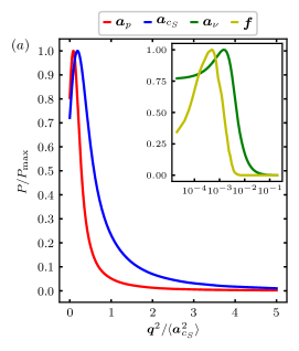
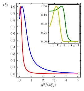
Figure 1: Probability density functions (PDFs) $P$ of Navier-Stokes acceleration and force magnitudes $\boldsymbol{q}^{2}$ for terms $\boldsymbol{q}$ listed at the top of $(a)$. $P_{\text{max}}$ for the PDF of $\boldsymbol{q}^{2}$ denotes its maximum value. $(a)$ $\langle\Rey_{\lambda}\rangle_{t}=112$, $(b)$ $\langle\Rey_{\lambda}\rangle_{t}=174$.

The DNS of Tsinober et al. (2001) showed that $\boldsymbol{a}_{\nu}$ is typically negligible (i.e. in a statistical sense, not everywhere at any time in the flow) compared to all the other acceleration terms in the Tsinober equations, namely $\boldsymbol{a}_{l}$, $\boldsymbol{a}_{c_{S}}$, $\boldsymbol{a}_{c_{I}}$ and $\boldsymbol{a}_{p}$. This is confirmed by our DNS results in tables 2-3 and in figure 1 which are for similar Reynolds numbers to those of Tsinober et al. (2001) and where we report rms values, and probabilities of various acceleration terms. It is worth noting that $\boldsymbol{a}_{\nu}$ is not everywhere always negligible, at these Reynolds numbers at least. For example, $|\boldsymbol{a}_{\nu}|>0.1|\boldsymbol{a}_{c_{S}}|$ in $44.1\%$ and $30.8\%$ of the space-time domain for our lower and higher Reynolds number respectively; and if we consider $|\boldsymbol{a}_{\nu}|>0.32|\boldsymbol{a}_{c_{S}}|$, this is satisfied in $6.8\%$ and $3.7\%$ of cases. Note that the DNS results of Tsinober et al. (2001) suggest that the viscous force typically decreases in magnitude compared to $\boldsymbol{a}_{c_{S}}$ as the Reynolds number increases and our results for our two Reynolds numbers agree with this trend. One may therefore expect the the first of the two Tsinober equations for homogeneous/periodic turbulence with the kind of forcing we consider here to typically reduce to

$$\boldsymbol{a}_{l}+\boldsymbol{a}_{c_{S}}\approx 0,$$ (10)

at high enough Reynold numbers, the approximation being valid in the sense that the neglected terms are significantly smaller than the retained ones in the majority of the flow for the majority of the time. There exist, however, some relatively rare spacio-temporal events where the neglegted viscous force and/or body force are significant (for example, as stated a few lines above, $|\boldsymbol{a}_{\nu}|$ is larger than $0.32|\boldsymbol{a}_{c_{S}}|$ in $6.8\%$ and $3.7\%$ of all spatio-temporal events for our lower and higher Reynolds numbers respectively) and where the right hand side of (10) is therefore not zero. In fact, many of these relatively rare events can be expected to account for some or even much of the average turbulence dissipation which is a sum of squares of fluctuating velocity gradients. More generally, one cannot use equation (10) to derive statistics of fluctuating velocity gradients, as in Tang et al. (2022) for example.

The second of the two Tsinober equations, namely

$$\boldsymbol{a}_{c_{I}}=\boldsymbol{a}_{p},$$ (11)

is exact everywhere and at any time and we keep it as it is.

$\langle\Rey_{\lambda}\rangle_{t}$	$\langle\cos$($\boldsymbol{a}_{c_{I}}$, $\boldsymbol{a}_{p})\rangle$	$\langle\cos$($\boldsymbol{a}$, $\boldsymbol{a}_{p})\rangle$	$\langle\cos$($\boldsymbol{a}_{l}$, $\boldsymbol{a}_{c_{S}})\rangle$	$\langle\cos$($\boldsymbol{a}_{l}$, $\boldsymbol{a}_{c})\rangle$	$\langle\cos$($\boldsymbol{a}_{c}$, $\boldsymbol{a}_{p})\rangle$
112	0.9999	0.972	-0.985	-0.726	0.388
174	0.9999	0.975	-0.990	-0.796	0.308

Table 4: NS average alignments $\langle\cos(\boldsymbol{q},\boldsymbol{p})\rangle$ for NS acceleration pairs $(\boldsymbol{q},\boldsymbol{p})$.

Equations (10)-(11) suggest similar magnitudes and strong alignment between $\boldsymbol{a}_{l}$ and $-\boldsymbol{a}_{c_{S}}$ and equal magnitudes as well as perfect alignment between $\boldsymbol{a}_{c_{I}}$ and $\boldsymbol{a}_{p}$. Such magnitudes and alignments were observed in the DNS of Tsinober et al. (2001) and are also strongly confirmed by our own DNS in table 4 ($\boldsymbol{a}_{c_{S}}$ and $\boldsymbol{a}_{c_{I}}$ are calculated on the basis of equation (44) in appendix A and aliasing errors associated with non-linear terms are removed by phase-shifting and truncation (Patterson & Orszag, 1971)). As suggested by previous DNS and experimental results (e.g. Tsinober et al. (2001); Chevillard et al. (2005); Yeung et al. (2006)), and as also supported by our own DNS results in tables 2 and 4, $\boldsymbol{a}\approx\boldsymbol{a}_{p}$ and $\langle\boldsymbol{a}_{l}^{2}\rangle/\langle\boldsymbol{a}^{2}\rangle\sim\langle\Rey_{\lambda}\rangle_{t}^{1/2}$ In fact, the scaling $\langle\boldsymbol{a}_{l}^{2}\rangle/\langle\boldsymbol{a}^{2}\rangle\sim\langle\Rey_{\lambda}\rangle_{t}^{1/2}$ follows from the analysis of Tennekes (1975) who expressed the concept of passive sweeping by pointing out that ”at high Reynolds number the dissipative eddies flow past an Eulerian observer in a time much shorter than the time scale which characterizes their own dynamics”. It then follows from equations (10)-(11), from $\langle\boldsymbol{a}_{l}^{2}\rangle/\langle\boldsymbol{a}^{2}\rangle\sim\langle\Rey_{\lambda}\rangle_{t}^{1/2}$ and from $\langle\boldsymbol{a}_{p}^{2}\rangle\approx\langle\boldsymbol{a}^{2}\rangle$ that $\langle\boldsymbol{a}_{c_{S}}^{2}\rangle/\langle\boldsymbol{a}_{c_{I}}^{2}\rangle\sim\langle\Rey_{\lambda}\rangle_{t}^{1/2}$ with increasing $\langle Re_{\lambda}\rangle_{t}$, i.e., $\boldsymbol{a}_{c}$ becomes increasingly solenoidal with increasing $\langle Re_{\lambda}\rangle_{t}$. In this way, the anti-alignment in (10) leads to an increasing anti-alignment tendency between $\boldsymbol{a}_{l}$ and $\boldsymbol{a}_{c}$ with increasing Reynolds number, which is consistent with the notion of passive sweeping of small eddies by large ones, i.e. the random Taylor hypothesis of Tennekes (1975). These observations and conclusions were all made by Tsinober et al. (2001) and their DNS who showed, in particular, that the Taylor length-based Reynolds number does not need to be so large to make them, and are now confirmed by our DNS in table 2.

As a final point, it is a general property of isotropic random vector fields $\boldsymbol{q}$ that $\langle\boldsymbol{q}_{I}(\boldsymbol{x},t)\cdot\boldsymbol{q}_{S}(\boldsymbol{x}+\boldsymbol{r},t)\rangle_{x}=0$ for any $\boldsymbol{r}$ (including $\boldsymbol{r}=0$), where $\langle...\rangle_{\boldsymbol{x}}$ signifies a spatial average (Monin et al., 1975). Thus, $\langle\boldsymbol{a}_{c}^{2}\rangle=\langle\boldsymbol{a}_{c_{I}}^{2}\rangle+\langle\boldsymbol{a}_{c_{S}}^{2}\rangle$ if the small-scale turbulence is isotropic. Both our DNS and the DNS of Tsinober et al. (2001) confirm this equality. From this equality and from (10), $\langle\boldsymbol{a}_{c_{S}}^{2}\rangle/\langle\boldsymbol{a}_{c_{I}}^{2}\rangle\sim\langle\Rey_{\lambda}\rangle_{t}^{1/2}$, (11), $\boldsymbol{a}\approx\boldsymbol{a}_{p}$ and $\langle\boldsymbol{a}^{2}\rangle\gg\langle\boldsymbol{a}_{\nu}^{2}\rangle\gg\langle\boldsymbol{f}^{2}\rangle$, we have all in all

$$\langle\boldsymbol{a}_{c}^{2}\rangle\geq\langle\boldsymbol{a}_{c_{S}}^{2}\rangle\approx\langle\boldsymbol{a}_{l}^{2}\rangle\gg\langle\boldsymbol{a}_{c_{I}}^{2}\rangle=\langle\boldsymbol{a}_{p}^{2}\rangle\approx\langle\boldsymbol{a}^{2}\rangle\gg\langle\boldsymbol{a}_{\nu}^{2}\rangle\gg\langle\boldsymbol{f}^{2}\rangle,$$ (12)

for large enough $\langle\Rey_{\lambda}\rangle_{t}$. The average magnitude ordering in (12) is confirmed in our DNS (see table 2) and the DNS of Tsinober et al. (2001) even though the Reynolds numbers of these DNS are moderate and so the difference between $\langle\boldsymbol{a}_{c_{I}}^{2}\rangle$ and $\langle\boldsymbol{a}_{l}^{2}\rangle$ is not so large. Tsinober’s way to formulate sweeping is encapsulated in $\langle\boldsymbol{a}_{c_{S}}^{2}\rangle\approx\langle\boldsymbol{a}_{l}^{2}\rangle\gg\langle\boldsymbol{a}_{c_{I}}^{2}\rangle=\langle\boldsymbol{a}_{p}^{2}\rangle\approx\langle\boldsymbol{a}^{2}\rangle$ and in the alignments implied by equations (10)-(11) which are also statistically confirmed by our DNS in table 4.

3.2 From one-point to two-point Navier-Stokes dynamics in periodic/homogeneous turbulence

The Navier-Stokes difference (NSD) equation at centroid $\boldsymbol{x}$ and separation vector $\boldsymbol{r}$ is derived by subtracting the Navier-Stokes (NS) equation at location $\boldsymbol{x}^{+}=\boldsymbol{x}+\boldsymbol{r}/2$ from the NS equation at location $\boldsymbol{x}^{-}=\boldsymbol{x}-\boldsymbol{r}/2$. Defining $\delta\boldsymbol{q}(\boldsymbol{x},\boldsymbol{r},t)\equiv\boldsymbol{q}(\boldsymbol{x}+\boldsymbol{r}/2,t)-\boldsymbol{q}(\boldsymbol{x}-\boldsymbol{r}/2,t)$ for any NS term $\boldsymbol{q}(\boldsymbol{x},t)$, the NSD equation (Hill, 2002) reads

$$\frac{\partial\delta\boldsymbol{u}}{\partial t}+\delta\boldsymbol{a}_{c}=-\frac{1}{\rho}\nabla_{\boldsymbol{x}}\delta p+\delta\boldsymbol{a}_{\nu}+\delta\boldsymbol{f},$$ (13)

The NSD equation governs the evolution of $\delta\boldsymbol{u}$, which can be thought of as pertaining to the momentum at scales smaller or comparable to $|\boldsymbol{r}|$. We derive the solenoidal NSD equation by subtracting equation (8) at $\boldsymbol{x}-\boldsymbol{r}/2$ from the same equation at $\boldsymbol{x}+\boldsymbol{r}/2$. The same operation is used to derive the irrotational NSD equation. The resulting equations read

$$\frac{\partial\delta\boldsymbol{u}}{\partial t}+\delta\boldsymbol{a}_{c_{S}} =\delta\boldsymbol{a}_{\nu}+\delta\boldsymbol{f}_{S},$$ (14)

$$\delta\boldsymbol{a}_{c_{I}} =-\frac{1}{\rho}\nabla_{\boldsymbol{x}}\delta p+\delta\boldsymbol{f}_{I},$$ (15)

where $\delta\boldsymbol{a}_{c_{S}}(\boldsymbol{x},\boldsymbol{r},t)\equiv\boldsymbol{a}_{c_{S}}(\boldsymbol{x}+\boldsymbol{r}/2,t)-\boldsymbol{a}_{c_{S}}(\boldsymbol{x}-\boldsymbol{r}/2,t)$ and $\delta\boldsymbol{a}_{c_{I}}(\boldsymbol{x},\boldsymbol{r},t)\equiv\boldsymbol{a}_{c_{I}}(\boldsymbol{x}+\boldsymbol{r}/2,t)-\boldsymbol{a}_{c_{I}}(\boldsymbol{x}-\boldsymbol{r}/2,t)$ and note that these terms refer to solenoidal and irrotational terms in $\boldsymbol{x}$-space rather than $\boldsymbol{r}$-space. The forcings we consider have no irrotational part and so $\delta\boldsymbol{f}_{I}=0$. At the moderate $\langle\Rey_{\lambda}\rangle_{t}$ of our DNS, the approximate equation (10) is valid in the sense explained in the text which accompanies it in the previous sub-section, i.e. for a majority of spacio-temporal events. If the magnitude of the separation vector $\boldsymbol{r}$ is not too small for viscosity to matter directly nor too large for the forcing to be directly present, we may safely subtract equation (10) at $\boldsymbol{x}-\boldsymbol{r}/2$ from equation (10) at $\boldsymbol{x}+\boldsymbol{r}/2$ to obtain an approximation to (14) for sufficiently high Reynolds number: this is the first of the two equations below where $\delta\boldsymbol{a}_{l}\equiv\partial\delta\boldsymbol{u}/\partial t$:

$$\delta\boldsymbol{a}_{l}+\delta\boldsymbol{a}_{c_{S}} \approx 0,$$ (16)

$$\delta\boldsymbol{a}_{c_{I}} =-\frac{1}{\rho}\nabla_{\boldsymbol{x}}\delta p.$$ (17)

The second equation, equation (17), follows directly from (15) with $\delta\boldsymbol{f}_{I}=0$ without any restriction on either $\boldsymbol{r}$ or Reynolds number and is exact.

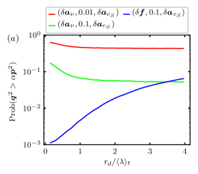
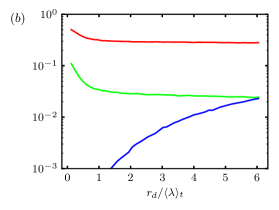
Figure 2: Navier-Stokes difference (NSD) exceedance probabilities $\text{Prob}(\boldsymbol{q}^{2}>\alpha\boldsymbol{p}^{2})$ for the NSD terms on top of ($a$) as a function of separation length $r_{d}=|\boldsymbol{r}|$. The legend entries read $(\boldsymbol{q},\alpha,\boldsymbol{p})$ for the NSD terms introduced in the first paragraph of 3.2. ($a$) $\langle\Rey_{\lambda}\rangle_{t}=112$, $\langle L\rangle_{t}=3.5\langle\lambda\rangle_{t}$. $(b)$ $\langle\Rey_{\lambda}\rangle_{t}=174$, $\langle L\rangle_{t}=5.2\langle\lambda\rangle_{t}$. NSD terms are sampled at scale $r_{d}=|\boldsymbol{r}|$ at random orientations $\boldsymbol{r}$.

Like equation (10), (16) can be expected to be valid broadly except where and when $\delta\boldsymbol{a}_{\nu}+\delta\boldsymbol{f}_{S}$ is large enough not to be negligible. Figure 2 shows statistically converged estimations of exceedance probabilities of NSD viscous and external force terms which suggest that (16) is indeed a good approximation for most of space and time at the Reynolds numbers of our two DNS, at the very least for separation distances larger than $\langle\lambda\rangle_{t}$ and smaller than $\langle L\rangle_{t}$. With regards to the forcing, $\text{Prob}(|\delta\boldsymbol{f}|>0.32|\delta\boldsymbol{a}_{c_{S}}|)$ is typically of the order of $1\%$, in particular for our higher Reynolds number. With regards to the viscous force, $\text{Prob}(|\delta\boldsymbol{a}_{\nu}|>0.32|\delta\boldsymbol{a}_{c_{S}}|)$ is typically of the order of $5\%$ for $r\geq\langle\lambda\rangle_{t}$ and even less for our higher Reynolds number.

The link between non-linearity and non-locality (via the pressure field) invoked in the two-point analysis of Yasuda & Vassilicos (2018) has its root in equation (17) which parallels (11) and states that $\delta\boldsymbol{a}_{c_{I}}$ and $\delta\boldsymbol{a}_{p}$ are perfectly aligned and have the same magnitudes. Furthermore, similarly to the way that equation (10) supports the concept of sweeping of small turbulent eddies by large ones in the usual one-point sense, (16) suggests similar magnitudes for and strong alignment between $\delta\boldsymbol{a}_{l}$ and $-\delta\boldsymbol{a}_{c_{S}}$. A two-point concept of sweeping similar to the one of Tennekes (1975) which relies on alignment between $\delta\boldsymbol{a}_{l}$ and $-\delta\boldsymbol{a}_{c}$ should also require that $\delta\boldsymbol{a}_{c}$ tends towards $\delta\boldsymbol{a}_{c_{s}}$ with increasing Reynolds number, i.e. that $\delta\boldsymbol{a}_{c}$ becomes increasingly solenoidal. We therefore seek to obtain inequalities and approximate equalities similar to (12). Note that equations (16)-(17) immediately imply $\langle\delta\boldsymbol{a}_{c_{S}}^{2}\rangle\approx\langle\delta\boldsymbol{a}_{l}^{2}\rangle$, $\langle\delta\boldsymbol{a}_{c_{I}}^{2}\rangle=\langle\delta\boldsymbol{a}_{p}^{2}\rangle$ and $\langle\delta\boldsymbol{a}_{p}^{2}\rangle\approx\langle\delta\boldsymbol{a}^{2}\rangle$. It therefore remains to argue that $\langle\delta\boldsymbol{a}_{c}^{2}\rangle\geq\langle\delta\boldsymbol{a}_{c_{S}}^{2}\rangle\gg\langle\delta\boldsymbol{a}_{c_{I}}^{2}\rangle$ which is exactly what we need to complete the new concept of two-point sweeping.

We start from

$$\langle\delta\boldsymbol{q}\cdot\delta\boldsymbol{q}\rangle(\boldsymbol{r}) =\langle\boldsymbol{q}^{+}\cdot\boldsymbol{q}^{+}\rangle-\langle\boldsymbol{q}^{+}\cdot\boldsymbol{q}^{-}\rangle+\langle\boldsymbol{q}^{-}\cdot\boldsymbol{q}^{-}\rangle-\langle\boldsymbol{q}^{-}\cdot\boldsymbol{q}^{+}\rangle,$$ (18)

$$=2\big{[}\langle\boldsymbol{q}\cdot\boldsymbol{q}\rangle-\langle\boldsymbol{q}^{+}\cdot\boldsymbol{q}^{-}\rangle(\boldsymbol{r})\big{]},$$ (19)

where $\boldsymbol{q}^{+}\equiv\boldsymbol{q}(\boldsymbol{x}+\boldsymbol{r}/2)$ and $\boldsymbol{q}^{-}\equiv\boldsymbol{q}(\boldsymbol{x}-\boldsymbol{r}/2)$ and where we used $\langle\boldsymbol{q}^{+}\cdot\boldsymbol{q}^{+}\rangle=\langle\boldsymbol{q}^{-}\cdot\boldsymbol{q}^{-}\rangle=\langle\boldsymbol{q}\cdot\boldsymbol{q}\rangle$ because of statistical homogeneity/periodicity. Previous studies (Hill & Thoroddsen, 1997; Vedula & Yeung, 1999; Xu et al., 2007; Gulitski et al., 2007) demonstrated that fluid accelerations, pressure-gradients and viscous forces have limited spatial correlations in terms of alignments at scales larger than $\langle\lambda\rangle_{t}$ for moderate and high $\langle\Rey_{\lambda}\rangle_{t}$. Thus, if we assume the two-point term to be negligible compared to the one-point term in Eq. (19) for scales $|\boldsymbol{r}|$ larger than $\langle\lambda\rangle_{t}$, we have that $\langle\delta\boldsymbol{q}\cdot\delta\boldsymbol{q}\rangle(\boldsymbol{r})$ is approximately equal to $2\langle\boldsymbol{q}\cdot\boldsymbol{q}\rangle$ for $|\boldsymbol{r}|$ larger than $\langle\lambda\rangle_{t}$. From (12) we therefore obtain

$$\langle\delta\boldsymbol{a}_{c}^{2}\rangle\geq\langle\delta\boldsymbol{a}_{c_{S}}^{2}\rangle\approx\langle\delta\boldsymbol{a}_{l}^{2}\rangle\gg\langle\delta\boldsymbol{a}_{c_{I}}^{2}\rangle=\langle\delta\boldsymbol{a}_{p}^{2}\rangle\approx\langle\delta\boldsymbol{a}^{2}\rangle\gg\langle\delta\boldsymbol{a}_{\nu}^{2}\rangle\gg\langle\delta\boldsymbol{f}^{2}\rangle,$$ (20)

for $|\boldsymbol{r}|$ larger than $\langle\lambda\rangle_{t}$, but $\langle\delta\boldsymbol{a}_{c}^{2}\rangle\geq\langle\delta\boldsymbol{a}_{c_{S}}^{2}\rangle$ and $\langle\delta\boldsymbol{a}_{c_{I}}^{2}\rangle=\langle\delta\boldsymbol{a}_{p}^{2}\rangle$ are in fact valid for any $\boldsymbol{r}$. Inequality $\langle\delta\boldsymbol{a}_{c}^{2}\rangle\geq\langle\delta\boldsymbol{a}_{c_{S}}^{2}\rangle$ follows from $\langle\delta\boldsymbol{a}_{c}^{2}\rangle=\langle\delta\boldsymbol{a}_{c_{I}}^{2}\rangle+\langle\delta\boldsymbol{a}_{c_{S}}^{2}\rangle$ which itself follows from $\langle\boldsymbol{a}_{c_{I}}(\boldsymbol{x},t)\cdot\boldsymbol{a}_{c_{S}}(\boldsymbol{x}+\boldsymbol{r},t)\rangle_{x}=0$ for any $\boldsymbol{r}$ if the turbulence is isotropic (Monin et al., 1975). Equality $\langle\delta\boldsymbol{a}_{c_{I}}^{2}\rangle=\langle\delta\boldsymbol{a}_{p}^{2}\rangle$ follows directly from (17) which is exact and holds for any $\boldsymbol{r}$ and any Reynolds number. Of equalities/inequalities (20), the ones that we did not already directly derive from/with equations (16)-(17) are $\langle\delta\boldsymbol{a}_{c}^{2}\rangle\geq\langle\delta\boldsymbol{a}_{c_{S}}^{2}\rangle\gg\langle\delta\boldsymbol{a}_{c_{I}}^{2}\rangle$ and $\langle\delta\boldsymbol{a}_{\nu}^{2}\rangle\gg\langle\delta\boldsymbol{f}^{2}\rangle$. The present way to formulate the new concept of two-point sweeping follows from Tsinober’s way to formulate sweeping and is encapsulated in $\langle\delta\boldsymbol{a}_{c_{S}}^{2}\rangle\approx\langle\delta\boldsymbol{a}_{l}^{2}\rangle\gg\langle\delta\boldsymbol{a}_{c_{I}}^{2}\rangle=\langle\delta\boldsymbol{a}_{p}^{2}\rangle\approx\langle\delta\boldsymbol{a}^{2}\rangle$ and in the alignments implied by equations (16)-(17). We confirm equations (16)-(17)-(20) with our DNS in the remainder of this subsection.

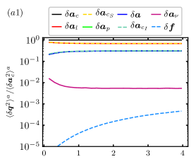
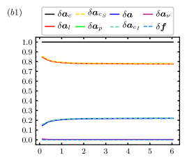
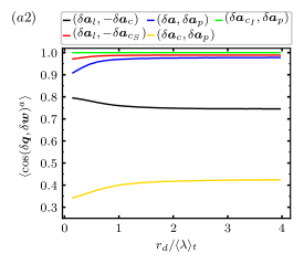
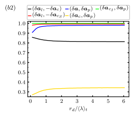
Figure 3: ($a1$,$b1$) spatio-temporal averages of spherically averaged NSD magntiudes $(\delta\boldsymbol{q}^{2})^{a}\equiv(\upi r_{d}^{2})^{-1}\iiint_{|\boldsymbol{r}|=r_{d}}\delta\boldsymbol{q}(\boldsymbol{x},\boldsymbol{r},t)\cdot\delta\boldsymbol{q}(\boldsymbol{x},\boldsymbol{r},t),\ d\boldsymbol{r}$ for NSD terms $\delta\boldsymbol{q}$ listed on top of the figures as a function of $r_{d}$: ($a1$) $\langle\Rey_{\lambda}\rangle_{t}=112$, ($b1$) $\langle\Rey_{\lambda}\rangle_{t}=174$. The magnitudes of the terms $\delta\boldsymbol{a}_{l}$ and $\delta\boldsymbol{a}_{c_{S}})$ overlap and the magntiudes of the terms $(\delta\boldsymbol{a}_{p}$, $\delta\boldsymbol{a}$ and $\delta\boldsymbol{a}_{c_{I}})$ also overlap. ($a2$, $b2$) average NSD alignments between NSD terms $(\delta\boldsymbol{q},\delta\boldsymbol{w})$ listed on top of the figures as a function of $r_{d}$: ($a2$) $\langle\Rey_{\lambda}\rangle_{t}=112$, ($b2$) $\langle\Rey_{\lambda}\rangle_{t}=174$.

To test (20) with our DNS data in a manageable way, we calculate spatio-temporal averages of $\boldsymbol{r}$-orientation-averaged quantities

$$(\delta\boldsymbol{q}\cdot\delta\boldsymbol{q})^{a}(\boldsymbol{x},r_{d},t)\equiv\frac{1}{\upi r_{d}^{2}}\iiint_{|\boldsymbol{r}|=r_{d}}\delta\boldsymbol{q}(\boldsymbol{x},\boldsymbol{r},t)\cdot\delta\boldsymbol{q}(\boldsymbol{x},\boldsymbol{r},t),\ d\boldsymbol{r},$$ (21)

which we plot in figure 3($a1$,$a2$) as ratios of such quantities versus two-point length $r_{d}$. In figure 3($a1$,$a2$) we plot spatio-temporal averages of $\boldsymbol{r}$-orientation-averaged quantities (21) for various acceleration/force terms in the NSD and the Helmholtz decomposed NSD equations. A comparison of relative magnitudes in the plots of figure 3($a1$,$a2$) with relative magnitudes in table 2 makes it clear that the results are consistent with (20) and $\langle\delta\boldsymbol{q}\cdot\delta\boldsymbol{q}\rangle(\boldsymbol{r})/\langle\boldsymbol{q}\cdot\boldsymbol{q}\rangle$ close to $2$ for $r_{d}\geq\langle\lambda\rangle_{t}$ at both $\langle Re_{\lambda}\rangle_{t}$ to a good degree of accuracy ($\langle\delta\boldsymbol{q}\cdot\delta\boldsymbol{q}\rangle(\boldsymbol{r})/\langle\boldsymbol{q}\cdot\boldsymbol{q}\rangle$ increases from 1.8 to 2.0 as $r_{d}$ grows from $\langle\lambda\rangle_{t}$ to $\langle L\rangle_{t}$). Note, in particular, that in Figure 3($a1$,$b1$) the average quantities corresponding to $\delta\boldsymbol{a}_{l}$ and $\delta\boldsymbol{a}_{c_{S}}$ overlap and those corresponding to $\delta\boldsymbol{a}_{p}$, $\delta\boldsymbol{a}$ and $\delta\boldsymbol{a}_{c_{I}}$ also overlap. At scales below $\langle\lambda\rangle_{t}$, the average relative magnitudes change slightly, but the NSD magnitude separations still abide by (20), the NSD analogue to (12), at all scales.

In figure 3($b1$,$b2$) we use our DNS data to plot spatio-temporal averages of $\boldsymbol{r}$-orientation-averaged cosines of angles between various NSD terms $\delta\boldsymbol{q}$ and $\delta\boldsymbol{w}$ to test for average alignments as a function of $r_{d}$. These alignment results are of course in perfect agreement with (17) but they are also in good agreement with (16) and acceptable agreement with $\delta\boldsymbol{a}\approx\delta\boldsymbol{a}_{p}$ (the cosine of the angle between these two acceleration vectors is higher than $0.9$ for all $r_{d}$). They also show that we should not expect $\delta\boldsymbol{a}_{l}$ to be extremely well aligned with $-\delta\boldsymbol{a}_{c}$ at our moderate Reynolds numbers. This demonstrates the pertinence of the solenoidal-irrotational decomposition which has revealed very good alignments at our moderate Reynolds numbers for which there are significantly weaker alignments without this decomposition.

In conclusion, figure 3 provides strong support for equations (16)-(17)-(20) which establish the two-point link between non-linearity and non-locality, and also a concept of two-point sweeping.

3.3 Interscale transfer and physical space transport accelerations

The convective non-linearity is responsible for non-linear turbulence transport through space and non-linear transfer through scales. We want to separate these two effects and therefore decompose the two-point non-linear acceleration term $\delta\boldsymbol{a}_{c}$ into an interscale transfer acceleration $\boldsymbol{a}_{\mathit{\Pi}}$ and a physical space transport acceleration $\boldsymbol{a}_{\mathcal{T}}$ (Hill, 2002), i.e $\delta\boldsymbol{a}_{c}=\boldsymbol{a}_{\mathit{\Pi}}+\boldsymbol{a}_{\mathcal{T}}$ with

$$\boldsymbol{a}_{\mathcal{T}}(\boldsymbol{x},\boldsymbol{r},t)=\frac{1}{2}(\boldsymbol{u}^{+}+\boldsymbol{u}^{-})\cdot\nabla_{\boldsymbol{x}}\delta\boldsymbol{u},\quad\boldsymbol{a}_{\mathit{\Pi}}(\boldsymbol{x},\boldsymbol{r},t)=\delta\boldsymbol{u}\cdot\nabla_{\boldsymbol{r}}\delta\boldsymbol{u}.$$ (22)

With this decomposition of the non-linear term, the NSD equation (13) reads

$$\frac{\partial\delta\boldsymbol{u}}{\partial t}+\boldsymbol{a}_{\mathit{\Pi}}+\boldsymbol{a}_{\mathcal{T}}=-\frac{1}{\rho}\nabla_{\boldsymbol{x}}\delta p+\delta\boldsymbol{a}_{\nu}+\delta\boldsymbol{f}.$$ (23)

We note relations $\boldsymbol{a}_{\mathit{\Pi}}=\delta\boldsymbol{a}_{C}+u^{+}_{j}\partial\boldsymbol{u}^{-}/\partial x^{-}_{j}-u^{-}_{j}\partial\boldsymbol{u}^{+}/\partial x^{+}_{j}$ and $\boldsymbol{a}_{\mathcal{T}}=\delta\boldsymbol{a}_{C}-u^{+}_{j}\partial\boldsymbol{u}^{-}/\partial x^{-}_{j}+u^{-}_{j}\partial\boldsymbol{u}^{+}/\partial x^{+}_{j}$ which can be easily used to show that $\langle\boldsymbol{a}_{\mathit{\Pi}}^{2}\rangle$ and $\langle\boldsymbol{a}_{\mathcal{T}}^{2}\rangle$ tend towards each other as the amplitude of the separation vector $\boldsymbol{r}$ grows above the integral length scale. We report DNS evidence of this tendency, below in this paper.

We want to consider the effects of the interscale transfer and interspace transport terms in the solenoidal and irrotational NSD dynamics and we therefore need to break down the NSD equation (23) into two equations, one irrotational and one solenoidal. We therefore perform Helmholtz decompositions in centroid space $\boldsymbol{x}$ for a given separation $\boldsymbol{r}$ at time $t$, for example $\delta\boldsymbol{q}(\boldsymbol{x},\boldsymbol{r},t)=\delta\boldsymbol{q}_{\overline{I}}(\boldsymbol{x},\boldsymbol{r},t)+\delta\boldsymbol{q}_{\overline{S}}(\boldsymbol{x},\boldsymbol{r},t)$ where $\delta\boldsymbol{q}_{\overline{I}}(\boldsymbol{x},\boldsymbol{r},t)$ and $\delta\boldsymbol{q}_{\overline{S}}(\boldsymbol{x},\boldsymbol{r},t)$ are, respectively, the irrotational and solenoidal parts in centroid space of $\delta\boldsymbol{q}(\boldsymbol{x},\boldsymbol{r},t)$. This decomposition in centroid space differs in general from the difference of the Helmholtz decomposed terms in the NS equations which gives equations (14)-(15), but in periodic/homogeneous turbulence $\delta\boldsymbol{q}_{I}=\delta\boldsymbol{q}_{{\overline{I}}}$ and $\delta\boldsymbol{q}_{S}=\delta\boldsymbol{q}_{{\overline{S}}}$ (see appendix B). Furthermore, from $\delta\boldsymbol{a}_{c}=\boldsymbol{a}_{\mathit{\Pi}}+\boldsymbol{a}_{\mathcal{T}}$ immediately follow $\delta\boldsymbol{a}_{c_{\overline{S}}}=\boldsymbol{a}_{\mathit{\Pi}_{\overline{S}}}+\boldsymbol{a}_{\mathcal{T}_{\overline{S}}}$ and $\delta\boldsymbol{a}_{c_{\overline{I}}}=\boldsymbol{a}_{\mathit{\Pi}_{\overline{I}}}+\boldsymbol{a}_{\mathcal{T}_{\overline{I}}}$. Thus, we can rewrite the NSD solenoidal and irrotational equations (14)-(15) as

$$\boldsymbol{a}_{\mathit{\Pi}_{\overline{I}}}+\boldsymbol{a}_{\mathcal{T}_{\overline{I}}} =\delta\boldsymbol{a}_{p},$$ (24)

$$\delta\boldsymbol{a}_{l}+\boldsymbol{a}_{\mathit{\Pi}_{\overline{S}}}+\boldsymbol{a}_{\mathcal{T}_{\overline{S}}} =\delta\boldsymbol{a}_{\nu}+\delta\boldsymbol{f},$$ (25)

in periodic/homogeneous turbulence.

We emphasize that the interscale transfer term $\boldsymbol{a}_{\mathit{\Pi}_{\overline{S}}}$ is related non-locally in space to two-point vortex stretching and compression terms governing the evolution of vorticity difference $\delta\boldsymbol{\omega}$. This follows from the fact that, as for the Tsinober equations, the NSD solenoidal equation is an integrated vorticity difference equation. We provide mathematical detail on the connection between $\boldsymbol{a}_{\mathit{\Pi}_{\overline{S}}}$ and $\delta\boldsymbol{\omega}$ in appendix C. This relation between $\boldsymbol{a}_{\mathit{\Pi}_{\overline{S}}}$ and the vorticity difference dynamics provides an instantaneous connection between the interscale momentum dynamics and two-point vorticity stretching and compression dynamics.

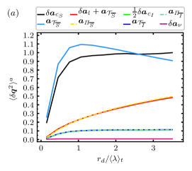
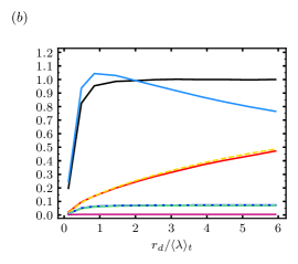
Figure 4: Average magnitudes $\langle\delta\boldsymbol{q}^{2}\rangle^{a}$ of NSD terms present in the irrotational and solenoidal NSD equations (25)-(26) listed on top of $(a)$. All values have been normalised with $\langle\delta\boldsymbol{a}_{c_{S}}^{2}\rangle^{a}$ at the largest considered separation $r_{d}$. The magnitudes of the terms $(\delta\boldsymbol{a}_{l}+\boldsymbol{a}_{\mathcal{T}_{\overline{S}}}$ and $\boldsymbol{a}_{\mathit{\Pi}_{\overline{S}}})$ overlap and the magnitudes of the terms $(1/2\delta\boldsymbol{a}_{c_{I}}$, $\boldsymbol{a}_{\mathcal{T}_{\overline{I}}}$ and $\boldsymbol{a}_{\mathit{\Pi}_{\overline{I}}})$ also overlap. ($a$) $\langle\Rey_{\lambda}\rangle_{t}=112$, ($b$) $\langle\Rey_{\lambda}\rangle_{t}=174$.

Equation (24) can also be obtained by integrating the Poisson equation for $\delta p$ in centroid space similarly to equation (25) which, as already mentioned, can be obtained by integrating the vorticity difference equation in that same space. We use this approach in appendix C to derive these equations for periodic/homogeneous turbulence but also their generalised form for non-homogeneous turbulence. By deriving the exact equations for $\boldsymbol{a}_{\mathcal{T}_{\overline{I}}}(\boldsymbol{x},\boldsymbol{r},t)$ and $\boldsymbol{a}_{\mathit{\Pi}_{\overline{I}}}(\boldsymbol{x},\boldsymbol{r},t)$ in Fourier centroid space we show in appendix B that we have $\boldsymbol{a}_{\mathcal{T}_{\overline{I}}}(\boldsymbol{x},\boldsymbol{r},t)=\boldsymbol{a}_{\mathit{\Pi}_{\overline{I}}}(\boldsymbol{x},\boldsymbol{r},t)$ in periodic/homogeneous turbulence. This result combined with (24) yields

$$\boldsymbol{a}_{\mathit{\Pi}_{\overline{I}}}=\boldsymbol{a}_{\mathcal{T}_{\overline{I}}}=\frac{1}{2}\delta\boldsymbol{a}_{p}=\frac{1}{2}\delta\boldsymbol{a}_{c_{I}},$$ (26)

in periodic/homogeneous turbulence. In figure 4 we plot spatio-temporal averages of $\boldsymbol{r}$-orientation-averaged quantities (21) for various acceleration/force terms in the NSD and the Helmholtz decomposed NSD equations and in figure 5 we plot spatio-temporal averages of $\boldsymbol{r}$-orientation-averaged cosines of angles between various two-point acceleration terms in these equations. The overlapping magnitudes in figure 4 and the average alignments in figure 5 confirm (26), or rather validate our DNS given that (26) is exact.

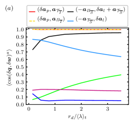
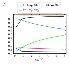
Figure 5: Average alignments of NSD terms $(\delta\boldsymbol{q},\delta\boldsymbol{w})$ listed on top of ($a$) and $(b)$. The average alignments of $(\delta\boldsymbol{a}_{p},\boldsymbol{a}_{\mathcal{T}_{\overline{I}}})$ and $(\delta\boldsymbol{a}_{p},\boldsymbol{a}_{\mathit{\Pi}_{\overline{I}}})$ overlap: ($a$) $\langle\Rey_{\lambda}\rangle_{t}=112$, ($b$) $\langle\Rey_{\lambda}\rangle_{t}=174$.

The computational procedure to calculate the various $\boldsymbol{r}$-orientation-averaged terms in these figures is computationally expensive. To calculate the NSD irrotational and solenoidal parts of the interscale and interspace transport terms at a given time $t$ and separation $\boldsymbol{r}$, we use the pseudo-spectral algorithm of Patterson & Orszag (1971) with one phase-shift and spherical truncation. We apply this algorithm to $\delta u_{j}$ and $\partial\delta u_{i}/\partial r_{j}$ for the interscale transfer and for $(u_{j}^{+}+u_{j}^{-})/2$ and $\partial\delta u_{i}/\partial x_{j}$ for the interspace transfer. Hence, we express these vectors/tensors in Fourier-space (see equations (61)-(64) in appendix B) and apply the pseudo-spectral method of Patterson & Orszag (1971) to calculate $\widehat{\boldsymbol{a}_{\mathcal{T}}}(\boldsymbol{k},\boldsymbol{r},t)$ and $\widehat{\boldsymbol{a}_{\mathit{\Pi}}}(\boldsymbol{k},\boldsymbol{r},t)$ without aliasing errors. We next decompose these fields to irrotational and solenoidal fields with the projection operator and inverse these fields to physical space to obtain $\boldsymbol{a}_{\mathit{\Pi}_{\overline{S}}}(\boldsymbol{x},\boldsymbol{r},t)$, $\boldsymbol{a}_{\mathit{\Pi}_{\overline{I}}}(\boldsymbol{x},\boldsymbol{r},t)$, $\boldsymbol{a}_{\mathcal{T}_{\overline{S}}}(\boldsymbol{x},\boldsymbol{r},t)$ and $\boldsymbol{a}_{\mathcal{T}_{\overline{I}}}(\boldsymbol{x},\boldsymbol{r},t)$. These fields can then be sampled over $\boldsymbol{x}$ to calculate e.g. $\boldsymbol{a}_{\mathit{\Pi}_{\overline{S}}}^{2}(\boldsymbol{x},\boldsymbol{r},t)$ or KHMH terms such as $2\delta\boldsymbol{u}\cdot\boldsymbol{a}_{\mathit{\Pi}_{\overline{S}}}(\boldsymbol{x},\boldsymbol{r},t)$ (see section 3.4). If we assume that the cost of a DNS time-step is similar to the cost of the pseudo-spectral method to calculate the NS non-linear term, the calculation of solenoidal and irrotational interspace and interscale transfers for one $t$ and one $\boldsymbol{r}$ has similar cost to one DNS time-step. The total cost of the pseudo-spectral post-processing method is proportional to the total number $N_{r}$ of separation vectors $\boldsymbol{r}$ that we use in our spherical averaging across scales $r_{d}$ and to the total number $T_{s}/\Delta T$ of samples in time (see table 1). With a total number of separation vectors $N_{r}\sim 10^{3}-10^{4}$ and our $T_{s}/\Delta T$ values, the total cost of the pseudo-spectral post-processing method in terms of DNS time-steps is at least one order of magnitude larger than the cost of the DNS itself. This high post-processing cost limits the $\langle\Rey_{\lambda}\rangle_{t}$ values of this study.

The NSD solenoidal equation (25) describes a balance between the time-derivative, solenoidal interscale transfer, solenoidal interspace transport, viscous and forcing terms. From the point we made in the sentence directly following equation (23), we expect $\langle\boldsymbol{a}_{\mathcal{T}_{\overline{S}}}^{2}\rangle$ and $\langle\boldsymbol{a}_{\mathit{\Pi}_{\overline{S}}}^{2}\rangle$ to tend to become equal to each other as the amplitude of $\boldsymbol{r}$ tends to values significantly larger than $\langle L\rangle_{t}$. Figure 4 confirms this trend for the orientation-averaged fluctuation magnitudes of $\boldsymbol{a}_{\mathcal{T}_{\overline{S}}}$ and $\boldsymbol{a}_{\mathit{\Pi}_{\overline{S}}}$. With decreasing $r_{d}$, $\langle\boldsymbol{a}_{\mathit{\Pi}_{\overline{S}}}^{2}\rangle^{a}$ decreases relative to $\langle\boldsymbol{a}_{\mathcal{T}_{\overline{S}}}^{2}\rangle$. At all scales $r_{d}\geq\langle\lambda\rangle_{t}$ the fluctuation magnitudes of $\boldsymbol{a}_{\mathcal{T}_{\overline{S}}}$ and $\boldsymbol{a}_{\mathit{\Pi}_{\overline{S}}}$ are one order of magnitude larger than those of the viscous term $\delta\boldsymbol{a}_{\nu}$ and this separation is greater for the larger $\langle\Rey_{\lambda}\rangle_{t}$. The fluctuation magnitudes of $\delta\boldsymbol{a}_{\nu}$ are themselves much larger than those of $\delta\boldsymbol{f}$ (not shown in figure 4 for not overloading the figure but see figure 3($a1$)). These observations suggest that the solenoidal NSD equation (25) reduces to the approximate

$$\delta\boldsymbol{a}_{l}+\boldsymbol{a}_{\mathcal{T}_{\overline{S}}}\approx-\boldsymbol{a}_{\mathit{\Pi}_{\overline{S}}},$$ (27)

where this equation is understood as typical in terms of fluctuation magnitudes: i.e. in most regions of the flow for the majority of the time, the removed terms are at least one order of magnitude smaller than the retained terms. (As for the NS dynamics, we do expect dynamically important regions localised in space and time where the dynamics differ from (27).) Figure 4 confirms equation (27) in this sense and shows that the relatively rare spatio-temporal events which are neglected when writing equation (27) are indeed present as the fluctuation magnitudes do show a very small deviation from equation (27). An additional important observation to be made from figure 4 is that $\delta\boldsymbol{a}_{c_{S}}$ tends to become increasingly dominated by $\boldsymbol{a}_{\mathcal{T}_{\overline{S}}}$ rather than $\boldsymbol{a}_{\mathit{\Pi}_{\overline{S}}}$ as $r_{d}$ decreases.

Equation (27) is the same as equation (16), and similarly to figure 3 which provides support for equation (16), figures 4 and 5 provide strong support for equation (27), in particular for $r_{d}>\langle\lambda\rangle_{t}$. It is interesting to note that the average alignment between the left and the right hand side of equation (27) lies between 90% and 100% (typically 95%) for $r_{d}>\langle\lambda\rangle_{t}$. Whilst this is strong support for approximate equation (27), the fact that the alignment is not 100% is a reminder of the nature of the approximation, i.e. that relatively rare spatio-temporal events do exist where the viscous and/or driving forces are not negligible.

At length-scales $r_{d}\leq\langle\lambda\rangle_{t}$, the alignment between $\delta\boldsymbol{a}_{l}$ and $-\boldsymbol{a}_{\mathcal{T}_{\overline{S}}}$ improves while the alignment between $\delta\boldsymbol{a}_{l}+\boldsymbol{a}_{\mathcal{T}_{\overline{S}}}$ and $-\boldsymbol{a}_{\mathit{\Pi}_{\overline{S}}}$ worsens with decreasing $r_{d}$ (see figure 5) presumably because of direct dissipation and diffusion effects, so that $\delta\boldsymbol{a}_{l}+\boldsymbol{a}_{\mathcal{T}_{\overline{S}}}\approx 0$ becomes a better approximation than equation (27) at $r_{d}<0.5\langle\lambda\rangle_{t}$. This observation is consistent with our parallel observation that the magnitude of $\boldsymbol{a}_{\mathcal{T}_{\overline{S}}}$ increases while the magnitude of $\boldsymbol{a}_{\mathit{\Pi}_{\overline{S}}}$ decreases with decreasing $r_{d}$ and that $\delta\boldsymbol{a}_{c_{S}}$ in equation (16) tends to be dominated by $\boldsymbol{a}_{\mathcal{T}_{\overline{S}}}$ at the very smallest scales.

On the other end of the spectrum, i.e. as the length scale $r_{d}$ grows towards $\langle L\rangle_{t}$, the alignment between $\delta\boldsymbol{a}_{l}$ and $-\boldsymbol{a}_{\mathcal{T}_{\overline{S}}}$ worsens while the alignment between $\delta\boldsymbol{a}_{l}$ and $-\boldsymbol{a}_{\mathit{\Pi}_{\overline{S}}}$ improves (see figure 5), both reaching a comparable level of alignment/misalignment which contribute together to keep approximation (27) statistically well satisfied with 95% alignment between $\delta\boldsymbol{a}_{l}+\boldsymbol{a}_{\mathcal{T}_{\overline{S}}}$ and $-\boldsymbol{a}_{\mathit{\Pi}_{\overline{S}}}$.

The strong anti-alignment between $\boldsymbol{a}_{\mathcal{T}_{\overline{S}}}$ and $\delta\boldsymbol{a}_{l}$, increasingly so at smaller $r_{d}$ (see figure 5) expresses the sweeping of the two-point momentum difference $\delta\boldsymbol{u}$ at scales $r_{d}$ and smaller by the mainly large scale velocity $(\boldsymbol{u}^{+}+\boldsymbol{u}^{-})/2$. Note that this two-point sweeping differs from anti-alignment between $\delta\boldsymbol{a}_{l}$ and $\delta\boldsymbol{a}_{c}$ for two reasons. Firstly, by using the Helmholtz decomposition we have removed the pressure effect embodied in the $\boldsymbol{a}_{c_{I}}$ contribution to $\boldsymbol{a}_{c}$ which balances the pressure-gradient. This was first understood in Tsinober et al. (2001) in a one-point setting and is here extended to a two-point setting. Secondly, $\delta\boldsymbol{a}_{c_{S}}$ is the sum of an interspace transport $\boldsymbol{a}_{\mathcal{T}_{\overline{S}}}$ and an interscale transfer term $\boldsymbol{a}_{\mathit{\Pi}_{\overline{S}}}$ such that the interpretation of two-point sweeping as anti-alignment between $\boldsymbol{a}_{c_{S}}$ and $\boldsymbol{a}_{l}$ as sweeping cannot be exactly accurate. The advection of $\delta\boldsymbol{u}$ by the large scale velocity is attributable to $\boldsymbol{a}_{\mathcal{T}_{\overline{S}}}$, and figure 5 shows that the two-point sweeping anti-alignment between $\delta\boldsymbol{a}_{l}$ and $\boldsymbol{a}_{\mathcal{T}_{\overline{S}}}$ increases with decreasing $r_{d}$.

The sweeping anti-alignment between $\delta\boldsymbol{a}_{l}$ and $\boldsymbol{a}_{\mathcal{T}_{\overline{S}}}$ is by no means perfect even if it reaches about 90% accuracy at $r_{d}<\langle\lambda\rangle_{t}$, as is clear from the similar magnitudes and very strong alignment tendency between $\delta\boldsymbol{a}_{l}+\boldsymbol{a}_{\mathcal{T}_{\overline{S}}}$ and $-\boldsymbol{a}_{\mathit{\Pi}_{\overline{S}}}$ at scales $|\boldsymbol{r}|\geq\langle\lambda\rangle_{t}$ (see figures 4 and 5). Note, in passing, that the Lagrangian solenoidal acceleration $\delta\boldsymbol{a}_{l}+\boldsymbol{a}_{\mathcal{T}_{\overline{S}}}$ and $\boldsymbol{a}_{\mathit{\Pi}_{\overline{S}}}$ are both Galilean invariant. Equation (27) may be interpreted to mean that the Lagrangian solenoidal acceleration of $\delta\boldsymbol{u}$ (which is actually solenoidal) moving with the mainly large scale velocity $(\boldsymbol{u}^{+}+\boldsymbol{u}^{-})/2$, namely $\delta\boldsymbol{a}_{l}+\boldsymbol{a}_{\mathcal{T}_{\overline{S}}}$, is evolving in time and space in response to $-\boldsymbol{a}_{\mathit{\Pi}_{\overline{S}}}$: when there is an influx of momentum from larger scales there is an increase in $\delta\boldsymbol{a}_{l}+\boldsymbol{a}_{\mathcal{T}_{\overline{S}}}$ and $\delta\boldsymbol{u}$ and vice versa.

3.4 From NSD dynamics to KHMH dynamics in homogeneous/periodic turbulence

The scale-by-scale evolution of $|\delta\boldsymbol{u}|^{2}$ locally in space and time is governed by a KHMH equation. This makes KHMH equations crucial tools for examining the turbulent energy cascade. The original KHMH equation and the new solenoidal and irrotational KHMH equations that we derive below are simply projections of the corresponding NSD equations onto $2\delta\boldsymbol{u}$. Hence, KHMH dynamics depend on NSD dynamics and the various NSD terms’ alignment or non-alignment tendencies with $2\delta\boldsymbol{u}$. In this subsection we present five KHMH results all clearly demarcated and identified in italics.

By contracting the NSD equation (13) with $2\delta\boldsymbol{u}$, one obtains the KHMH equation (Hill, 2002; Yasuda & Vassilicos, 2018):

$$\frac{\partial}{\partial t}|\delta\boldsymbol{u}|^{2}+\frac{u_{k}^{+}+u_{k}^{-}}{2}\frac{\partial}{\partial x_{k}}|\delta\boldsymbol{u}|^{2}+\frac{\partial}{\partial r_{k}}\big{(}\delta u_{k}|\delta\boldsymbol{u}|^{2}\big{)}=-\frac{2}{\rho}\frac{\partial}{\partial x_{k}}\big{(}\delta u_{k}\delta p\big{)}+2\nu\frac{\partial^{2}}{\partial r_{k}^{2}}|\delta\boldsymbol{u}|^{2}\\ +\frac{\nu}{2}\frac{\partial^{2}}{\partial x_{k}^{2}}|\delta\boldsymbol{u}|^{2}-\bigg{[}2\nu\big{(}\frac{\partial u_{i}^{+}}{\partial x_{k}^{+}}\big{)}^{2}+2\nu\big{(}\frac{\partial u_{i}^{-}}{\partial x_{k}^{-}}\big{)}^{2}\bigg{]}+2\delta u_{k}\delta f_{k},$$ (28)

where no fluid velocity decomposition nor averaging operations have been used. In line with the naming convention of Yasuda & Vassilicos (2018) this equation can be written

$$\mathcal{A}_{t}+\mathcal{T}+\mathit{\Pi}=\mathcal{T}_{p}+\mathcal{D}_{r,\nu}+\mathcal{D}_{x,\nu}-\mathcal{\epsilon}+\mathcal{I},$$ (29)

where the first, second and third terms on the left hand sides of equations (28) and (29) correspond to each other and so do the first, second, third, fourth and fifth terms on the right hand sides. Preempting notation used further down in this paper, equation (29) is also written $\mathcal{A}=\mathcal{T}_{p}+\mathcal{D}+\mathcal{I}$ or $\mathcal{A}_{t}+\mathcal{A}_{c}=\mathcal{T}_{p}+\mathcal{D}+\mathcal{I}$ where $\mathcal{A}_{c}\equiv\mathcal{T}+\mathit{\Pi}$, $\mathcal{A}\equiv\mathcal{A}_{t}+\mathcal{A}_{c}$ and $\mathcal{D}\equiv\mathcal{D}_{r,\nu}+\mathcal{D}_{x,\nu}-\mathcal{\epsilon}$.

To examine the KHMH dynamics in terms of irrotational and solenoidal dynamics we contract the irrotational and solenoidal NSD equations with $2\delta\boldsymbol{u}$ to derive what we refer to as irrotational and solenoidal KHMH equations. Each of the KHMH terms can be subdivided into a contribution from the NSD irrotational part and a contribution from the NSD solenoidal part of the respective term in the NSD equation. A solenoidal KHMH term corresponding to a $\delta\boldsymbol{q}(\boldsymbol{x},\boldsymbol{r},t)$ or $\boldsymbol{q}(\boldsymbol{x},\boldsymbol{r},t)$ term in equation (25) equals $\mathcal{Q}_{\overline{S}}=2\delta\boldsymbol{u}\cdot\delta\boldsymbol{q}_{\overline{S}}$ or $\mathcal{Q}_{\overline{S}}=2\delta\boldsymbol{u}\cdot\boldsymbol{q}_{\overline{S}}$, and an irrotational KHMH term corresponding to a $\delta\boldsymbol{q}(\boldsymbol{x},\boldsymbol{r},t)$ or $\boldsymbol{q}(\boldsymbol{x},\boldsymbol{r},t)$ term in equation (26) equals $\mathcal{Q}_{\overline{I}}=2\delta\boldsymbol{u}\cdot\delta\boldsymbol{q}_{\overline{I}}$ or $\mathcal{Q}_{\overline{I}}=2\delta\boldsymbol{u}\cdot\boldsymbol{q}_{\overline{I}}$. With $\mathcal{Q}=2\delta\boldsymbol{u}\cdot\delta\boldsymbol{q}$ or $\mathcal{Q}=2\delta\boldsymbol{u}\cdot\boldsymbol{q}$, we have $\mathcal{Q}=\mathcal{Q}_{\overline{I}}+\mathcal{Q}_{\overline{S}}$. The irrotational and solenoidal KHMH equations for periodic/homogeneous turbulence follow from equations (25) and (26) respectively and read

$$\mathcal{A}_{t}+\mathcal{T}_{\overline{S}}+\mathit{\Pi}_{\overline{S}} =\mathcal{D}_{r,\nu}+\mathcal{D}_{x,\nu}-\mathcal{\epsilon}+\mathcal{I},$$ (30)

$$\mathit{\Pi}_{\overline{I}}=\mathcal{T}_{\overline{I}} =\frac{1}{2}\mathcal{T}_{p},$$ (31)

where use has been made of the fact that the velocity and velocity difference fields are solenoidal. These two equations are our first KHMH result.

Space-local changes in time of $|\delta\boldsymbol{u}|^{2}$, expressed via $\mathcal{A}_{t}$, are only due to solenoidal KHMH dynamics in equation (30) which include interspace transport, interscale transport, viscous and forcing effects. The irrotational KHMH equation (31) formulates how the imposition of incompressibility by the pressure field affects interspace and interscale dynamics and, in turn, energy cascade dynamics. Generalised solenoidal and irrotational KHMH equations also valid for non-periodic/non-homogeneous turbulence are given in appendix C.

We first consider the spatio-temporal average of these equations in statistically steady forced periodic/homogeneous turbulence. As $\langle\mathcal{T}_{p}\rangle=0$, we obtain from equation (31), $\langle\mathit{\Pi}_{\overline{I}}\rangle=\langle\mathcal{T}_{\overline{I}}\rangle=0$. As $\langle\mathcal{T}_{\overline{S}}\rangle+\langle\mathcal{T}_{\overline{I}}\rangle=\langle\mathcal{T}\rangle=0$, we have $\langle\mathcal{T}_{\overline{S}}\rangle=0$, such that the spatio-temporal average of (30) reads

$$\langle\mathit{\Pi}\rangle=\langle\mathit{\Pi}_{\overline{S}}\rangle=\langle\mathcal{D}_{r,\nu}\rangle-\langle\mathcal{\epsilon}\rangle+\langle\mathcal{I}\rangle.$$ (32)

If an intermediate inertial subrange of scales $|\boldsymbol{r}|$ can be defined where viscous diffusion and forcing are negligible, equation (32) reduces to $\langle\mathit{\Pi}_{\overline{S}}\rangle\approx-\langle\mathcal{\epsilon}\rangle$ in that range. This theoretical conclusion (which is not part of our DNS study) is the backbone of the Kolmogorov (1941a, b, c) theory for high Reynolds number statistically homogeneous stationary small-scale turbulence with the additional information that the part of the average interscale transfer rate involved in Kolmogorov’s equilibrium balance is the solenoidal interscale transfer rate only. This is our second KHMH result. On average, there is a cascade of turbulence energy from large to small scales where the rate of interscale transfer is dominated by two-point vortex stretching (see appendix C for the relation between the solenoidal interscale transfer and vortex stretching) and is equal to $-\langle\mathcal{\epsilon}\rangle$ independently of $|\boldsymbol{r}|$ over a range of scales where viscous diffusion and forcing are negligible.

In this paper we concentrate on the fluctuations around the average picture described by the scale-by-scale equilibrium (32) for any Reynolds number. If we subtract the spatio-temporal average solenoidal KHMH equation (32) from the solenoidal KHMH equation (30) and use the generic notation $\mathcal{Q}^{{}^{\prime}}\equiv\mathcal{Q}-\langle\mathcal{Q}\rangle$, we attain the fluctuating solenoidal KHMH equation

$$\mathcal{A}_{t}+\mathcal{T}_{\overline{S}}+\mathit{\Pi}_{\overline{S}}^{{}^{\prime}}=\mathcal{D}_{r,\nu}^{{}^{\prime}}+\mathcal{D}_{x,\nu}-\mathcal{\epsilon}^{{}^{\prime}}+\mathcal{I}^{{}^{\prime}}.$$ (33)

This equation governs the fluctuations of the KHMH solenoidal dynamics around its spatio-temporal average. Clearly, if these non-equilibrium fluctuations are large relative to their average values, the average picture expressed by equation (32) is not characteristic of the interscale transfer dynamics. We now study the KHMH fluctuations in statistically stationary periodic/homogeneous turbulence on the basis of equations (31) and (33). Concerning equation (31), note that $\mathit{\Pi}_{\overline{I}}^{{}^{\prime}}=\mathit{\Pi}_{\overline{I}}$, $\mathcal{T}_{\overline{I}}^{{}^{\prime}}=\mathcal{T}_{\overline{I}}$ and $\mathcal{T}_{p}^{{}^{\prime}}=\mathcal{T}_{\overline{p}}$.

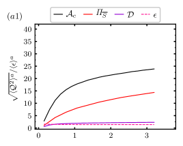
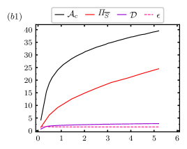
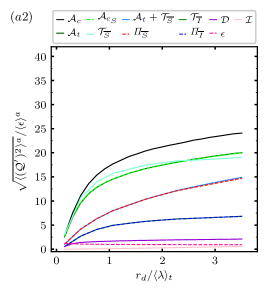
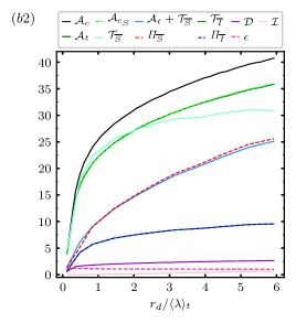
Figure 6: ($a1$, $b1$) KHMH average square magnitudes $\langle\mathcal{Q}^{2}\rangle^{a}$ and ($a2$, $b2$) KHMH average square fluctuating magnitudes $\langle(\mathcal{Q}^{{}^{\prime}})^{2}\rangle^{a}$, where $\mathcal{Q}^{{}^{\prime}}=\mathcal{Q}-\langle\mathcal{Q}\rangle$, for the KHMH terms $\mathcal{Q}$ listed above the figures and introduced in the third and fourth paragraph of 3.4. All entries are normalised with $\langle\mathcal{\epsilon}\rangle^{a}$ (see equations (28)-(29)). The following pairs of KHMH terms have overlapping magnitudes in $(a2,b2)$: $\mathcal{A}_{t}$ and $\mathcal{A}_{c_{S}}$; $\mathcal{A}_{t}+\mathcal{T}_{\overline{S}}$ and $\mathit{\Pi}_{\overline{S}}$; $\mathcal{T}_{\overline{I}}$ and $\mathit{\Pi}_{\overline{I}}$. ($a1$, $a2$) $\langle\Rey_{\lambda}\rangle_{t}=112$, ($b1$,$b2$) $\langle\Rey_{\lambda}\rangle_{t}=174$.

We start by determining the relative fluctuation magnitudes of the spatio-temporal fluctuations of each term in the KHMH equations (31) and (33). These relative fluctuation magnitudes can emulate those of respective terms in the NSD equations under the following sufficient conditions: (i) the fluctuations are so intense that they dwarf averages, so that $\langle(\mathcal{Q}^{\prime})^{2}\rangle\approx\langle\mathcal{Q}^{2}\rangle$; (ii) the mean square of any KHMH term $\mathcal{Q}=2\delta\boldsymbol{u}\cdot\delta\boldsymbol{q}$ corresponding to a NSD term $\delta\boldsymbol{q}(\boldsymbol{x},\boldsymbol{r},t)$ (equivalently $\mathcal{Q}=2\delta\boldsymbol{u}\cdot\boldsymbol{q}$ corresponding to $\boldsymbol{q}(\boldsymbol{x},\boldsymbol{r},t)$) can be approximated as

$${\langle\mathcal{Q}^{2}\rangle(\boldsymbol{r})\approx 4\langle|\delta\boldsymbol{u}|^{2}\rangle\langle|\delta\boldsymbol{q}|^{2}\rangle\langle\text{cos}^{2}(\theta_{q})\rangle,}$$ (34)

where the approximate equality results from a degree of decorrelation and $\theta_{q}$ is the angle between $\delta\boldsymbol{q}(\boldsymbol{x},\boldsymbol{r},t)$ (or $\boldsymbol{q}(\boldsymbol{x},\boldsymbol{r},t)$) and $\delta\boldsymbol{u}(\boldsymbol{x},\boldsymbol{r},t)$; (iii) $\langle\text{cos}^{2}(\theta_{q})\rangle$ is not very sensitive to the choice of NSD term $\delta\boldsymbol{q}$ (or $\boldsymbol{q}$). Under these conditions, we get

$${\frac{\langle(2\delta\boldsymbol{u}\cdot\delta\boldsymbol{q})^{2}\rangle(\boldsymbol{r})}{\langle(2\delta\boldsymbol{u}\cdot\delta\boldsymbol{w})^{2}\rangle(\boldsymbol{r})}\approx\frac{\langle|\delta\boldsymbol{u}|^{2}\rangle\langle|\delta\boldsymbol{q}|^{2}\rangle\langle\text{cos}^{2}(\theta_{q})\rangle(\boldsymbol{r})}{\langle|\delta\boldsymbol{u}|^{2}\rangle\langle|\delta\boldsymbol{w}|^{2}\rangle\langle\text{cos}^{2}(\theta_{w})\rangle(\boldsymbol{r})}\approx\frac{\langle|\delta\boldsymbol{q}|^{2}\rangle(\boldsymbol{r})}{\langle|\delta\boldsymbol{w}|^{2}\rangle(\boldsymbol{r})}},$$ (35)

which means that KHMH relative fluctuation magnitudes and NSD relative fluctuation magnitudes are approximately identical. The first approximate equality in (35) follows directly from (34) and the second approximate equality follows from hypothesis (iii) that $\text{cos}^{2}(\theta_{q})$ and $\text{cos}^{2}(\theta_{w})$ are about equal.

We test hypothesis (i) by comparing the plots in figure 6($a1$, $b1$) with those in figure 6($a2$, $b2$). Figure 6($a1$, $b1$) shows average magnitudes of KHMH spatio-temporal fluctuations for terms with non-zero spatio-temporal averages. Comparing with figure 6($a2$, $b2$), we find $\langle(\mathcal{Q}^{\prime})^{2}\rangle^{a}\approx\langle\mathcal{Q}^{2}\rangle^{a}$, i.e. hypothesis (i), for all four terms plotted in figure 6($a1$, $b1$) at all length scales $r_{d}$ considered. Note that this does not hold for $\mathcal{D}_{r,\nu}^{{}^{\prime}}$ and $\mathcal{I}^{{}^{\prime}}$ which are the only KHMH fluctuations such that $\sqrt{\langle(\mathcal{Q}^{\prime})^{2}\rangle^{a}}/\langle\mathcal{\epsilon}\rangle^{a}$ is smaller (in fact significantly smaller) than $1$ at all scales. Figure 6 makes it also clear that the magnitudes of the fluctuations of all other KHMH terms (solenoidal and irrotational) are much higher than those of the turbulence dissipation at all scales $r_{d}>0.5\langle\lambda\rangle_{t}$, and more so for the higher of the two Reynolds numbers. For scales $r_{d}\geq\langle\lambda\rangle_{t}$, the largest average fluctuating magnitudes are those of $\mathcal{A}_{c}^{{}^{\prime}}$, followed closely by $\mathcal{A}_{t}$ and $\mathcal{T}_{\overline{S}}$. Next come the magnitudes of $\mathit{\Pi}_{\overline{S}}^{{}^{\prime}}$ and $\mathcal{A}_{t}+\mathcal{T}_{\overline{S}}$. Thereafter follow the irrotational terms $\mathit{\Pi}_{\overline{I}}=\mathcal{T}_{\overline{I}}$ $(=0.5\mathcal{T}_{p})$ and finally the viscous, dissipative and forcing terms $\mathcal{D}^{{}^{\prime}},\mathcal{\epsilon}^{{}^{\prime}}$ and $\mathcal{I}^{{}^{\prime}}$ in that order. This order of fluctuations is our third KHMH result. An average description of the interscale turbulent energy transfer dynamics in terms of its spatio-temporal average cannot, therefore, be accurate. In order to characterise these dynamics, attention must be directed at most if not all KHMH term fluctuations, and in fact to much more than just the turbulence dissipation fluctuations given that they are among the weakest.

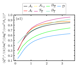
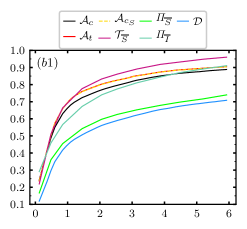
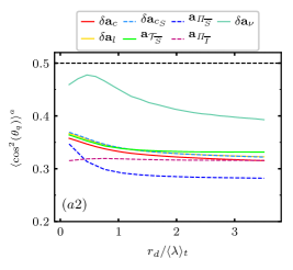
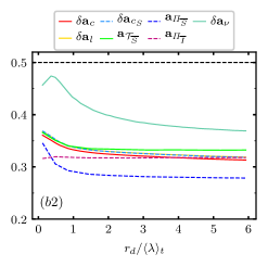
Figure 7: Test of the assumptions (ii) and (iii) in the seventh paragraph of subsection 3.4 related to relations (34)-(35) connecting NSD and KHMH relative magnitudes. ($a1$,$b1$) Test of assumption (ii) by taking the ratio of the left-hand and right-hand sides of (34) for the KHMH terms $\mathcal{Q}$ listed above the figures. ($a2$,$b2$) test of assumption (iii) used in (35) by comparing the behaviour of $\langle\cos^{2}(\theta_{q})\rangle^{a}$ for the various NSD terms listed above the figures. The black horizontal line $0.5$ corresponds to the value of $\langle\cos^{2}(\theta_{q})\rangle$ if $\theta_{q}$ is uniformly distributed. ($a1,a2$) $\langle\Rey_{\lambda}\rangle_{t}=112$, ($b1,b2$) $\langle\Rey_{\lambda}\rangle_{t}=174$.

Next, we test hypothesis (ii) by testing the validity of (34) and hypothesis (iii) concerning approximately similar $\text{cos}^{2}(\theta_{q})$ behaviour for different KHMH terms. In figure 7($a1$, $b1$) we plot ratios of right hand sides to left hand sides of equation (34) and see that (34) is not valid, but that it is nevertheless about 65% to 98% accurate for $r_{d}\geq\langle\lambda\rangle_{t}$. Note that (34) might be sufficient but that it is by no means necessary for the left-most and the right-most sides of (35) to approximately balance. In those cases where the variations between the ratios plotted in figure 7($a1$, $b1$) are not too large and the assumption of approximately similar $\text{cos}^{2}(\theta_{q})$ for different KHMH terms more or less holds, the left-most and the right-most sides of (35) can approximately balance.

Incidentally, figure 7($a2$, $b2$) also shows that the angles $\theta_{q}$ are not random but that they are more likely to be small rather than large in an approximately similar way for all important NSD terms: $\text{cos}^{2}(\theta_{q})$ ranges between about 0.28 and 0.36 for all NSD terms (except the viscous acceleration difference and the viscous force difference) at all scales $r_{d}$. These values are much smaller than 0.5, the value that $\text{cos}^{2}(\theta_{q})$ would have taken if the angles $\theta_{q}$ were random. There is therefore an alignment tendency between $\delta\boldsymbol{u}$ and NSD terms which is similar for all the important NSD terms, thereby allowing the balance between the left-most (ratio of KHMH terms) and the right-most (ratio of NSD terms) sides of (35) to approximately hold as seen by comparing the plots ($a1$)-($b1$) (mean square NSD terms) with the plots ($a2$)-($b2$) (mean square KHMH terms) in figure 8. (Note that the viscous term is bounded from above, $\langle\mathcal{D}^{2}\rangle(\boldsymbol{r})\leq 4\langle|\delta\boldsymbol{u}|^{2}|\delta\boldsymbol{a}_{\nu}|^{2}\rangle$, which indicates limited magnitudes compared to the irrotational and the dominant solenoidal terms because of the limited magnitude of $\langle\delta\boldsymbol{a}_{\nu}^{2}\rangle$. The limited fluctuations of the viscous terms are clearly seen in figure 6.)

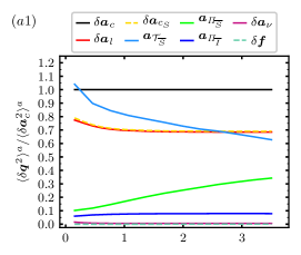
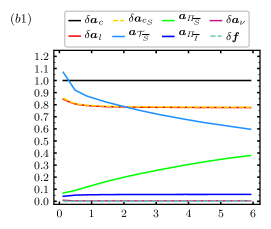
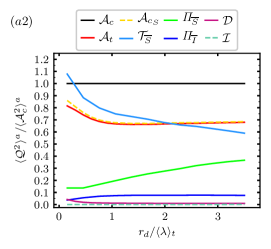
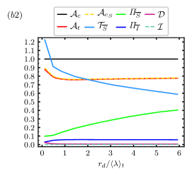
Figure 8: NSD and KHMH relative average square magnitudes (which should be similar on the basis of (35)) for the terms listed above the figures: ($a1$) NSD and ($a2$) KHMH for $\langle\Rey_{\lambda}\rangle_{t}=112$, ($b1$) NSD and ($b2$) KHMH for $\langle\Rey_{\lambda}\rangle_{t}=174$.

Figure 8 does indeed confirm the close correspondence between NSD and KHMH statistics which is a significant step further from the correspondence reported earlier in this paper between NS and NSD statistics. We can therefore use the approximate NSD relation (27) to deduce the following approximate KHMH relation:

$$\mathcal{A}_{t}+\mathcal{T}_{\overline{S}}+\mathit{\Pi}_{\overline{S}}^{{}^{\prime}} \approx 0,$$ (36)

understood in the sense that it holds in the majority of the domain for the majority of the time but that there surely exist relatively rare events within the flow where this approximate KHMH relation is violated.

This approximate equation $\mathcal{A}_{t}+\mathcal{T}_{\overline{S}}+\mathit{\Pi}_{\overline{S}}^{{}^{\prime}}\approx 0$ can be considered to be our fourth KHMH result. It is consistent with the order of fluctuation magnitudes in figure 8 which shows, in agreement with the NSD - KHMH correspondence just established, that the largest fluctuating magnitudes are those of $\mathcal{A}_{c}$, followed by the fluctuating magnitudes of $\mathcal{T}_{\overline{S}}$, $\mathcal{A}_{t}$ and $\mathcal{A}_{c_{S}}$ ($\mathcal{A}_{c_{S}}=\mathcal{T}_{\overline{S}}+\mathit{\Pi}_{\overline{S}}$). Note though that there is a cross over at about $r_{d}\approx 2\langle\lambda\rangle_{t}$ for both Reynolds numbers considered here between the fluctuation magnitudes of $\mathcal{T}_{\overline{S}}$ and those of $\mathcal{A}_{t}$ and $\mathcal{A}_{c_{S}}$ which are about equal to each other in agreement with equation (36).

The fluctuation magnitudes of $\mathit{\Pi}_{\overline{S}}$ and $\mathit{\Pi}_{\overline{I}}$ are both smaller than those just mentioned, and those of $\mathit{\Pi}_{\overline{I}}$ are significantly smaller than those of $\mathit{\Pi}_{\overline{S}}$. Even smaller, are the fluctuation magnitudes of $\mathcal{D}$ and $\mathcal{I}$, in that order. In agreement with (20), our third and fourth KHMH conclusions incorporate the following:

$$\langle\mathcal{A}_{t}^{2}\rangle\approx\langle\mathcal{A}_{c_{S}}^{2}\rangle\gg\langle\mathcal{T}_{p}^{2}\rangle=4\langle\mathit{\Pi}_{\overline{I}}^{2}\rangle=4\langle\mathcal{T}_{\overline{I}}^{2}\rangle=\langle\mathcal{A}_{c_{I}}^{2}\rangle\gg\langle\mathcal{D}^{2}\rangle\gg\langle\mathcal{I}^{2}\rangle,$$ (37)

where $\mathcal{A}_{c_{I}}=\mathcal{T}_{\overline{I}}+\mathit{\Pi}_{\overline{I}}$.

An additional significant observation from figure 8 which we can count as our fifth KHMH result is that, as $r_{d}$ decreases towards about $0.5\langle\lambda\rangle_{t}$, the fluctuation magnitude of $\mathcal{A}_{c_{S}}=\mathcal{T}_{\overline{S}}+\mathit{\Pi}_{\overline{S}}$ remains about constant but that of $\mathcal{T}_{\overline{S}}$ increases while that of $\mathit{\Pi}_{\overline{S}}$ decreases. (At scale $r_{d}$ smaller than $0.5\langle\lambda\rangle_{t}$, the fluctuation magnitudes of both $\mathcal{A}_{c_{S}}$ and $\mathcal{T}_{\overline{S}}$ increase with diminishing $r_{d}$ whereas those of $\mathit{\Pi}_{\overline{S}}$ remain about constant.) The convective non-linearity is increasingly of the spatial transport type and diminishingly of the interscale transfer type as the two-point separation length decreases.

We now consider correlations between different intermediate and large scale fluctuating KHMH terms in light of equations (31) and (36).

4 Fluctuating KHMH dynamics in homogeneous/periodic turbulence

4.1 Correlations

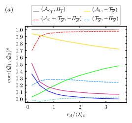
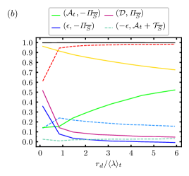
Figure 9: Spherically averaged correlation coefficients between KHMH terms $(\mathcal{Q}_{1},\mathcal{Q}_{2})$ listed above the plots $(a)$ and $(b)$. They are plotted as functions of scale $r_{d}$. ($a$) $\langle\Rey_{\lambda}\rangle_{t}=112$, ($b$) $\langle\Rey_{\lambda}\rangle_{t}=174$.

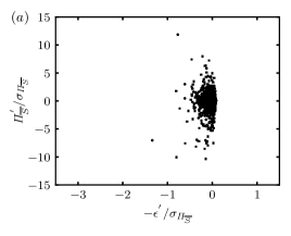
Figure 10: Scatter plots of $\mathit{\Pi}_{\overline{S}}^{{}^{\prime}}$ and $\-\mathcal{\epsilon}^{{}^{\prime}}$ at random orientations $\boldsymbol{r}$ with $r_{d}/\langle\lambda\rangle_{t}=(1.45,3.1)$ for $(a,b)$, $\sigma_{\mathit{\Pi}_{\overline{S}}}$ is the standard deviation of $\mathit{\Pi}_{\overline{S}}$ and $\langle\Rey_{\lambda}\rangle_{t}=174$.

We start this section by assessing the existence or non-existence of local (in space and time) equilibrium between interscale transfer and dissipation at some intermediate scales. In figure 9 we plot correlations between various KHMH terms. In particular, this figure shows that the correlation coefficient between $\mathit{\Pi}_{\overline{S}}^{{}^{\prime}}$ and $-\mathcal{\epsilon}^{{}^{\prime}}$ lies well below $0.1$ for all scales $r_{d}\geq\langle\lambda\rangle_{t}$. The scatter plots of these quantities in figure 10 confirm the absence of local relation between interscale transfer rate and dissipation rate. For example, for a given local/instantaneous dissipation fluctuation, the corresponding local/instantaneous interscale transfer rate fluctuation can be close to equally positive or negative. There is no local equilibrium between these quantities as they fluctuate at scales $r_{d}\geq\langle\lambda\rangle_{t}$. Such a correlation should of course not necessarily be expected. However, as $r_{d}$ decreases below $\langle\lambda\rangle_{t}$, the correlations between $\mathit{\Pi}_{\overline{S}}^{{}^{\prime}}$ and either $-\mathcal{\epsilon}^{{}^{\prime}}$ or $\mathcal{D}^{{}^{\prime}}$ increase up to values between about $0.3$ and about $0.5$. This increased correlation may suggest a feeble tendency towards local/instantaneous equilibrium between interscale transfer rate and dissipation rate at scales $r_{d}<\langle\lambda\rangle_{t}$. However, these scales are strongly affected by direct viscous processes and can therefore not be inertial range scales.

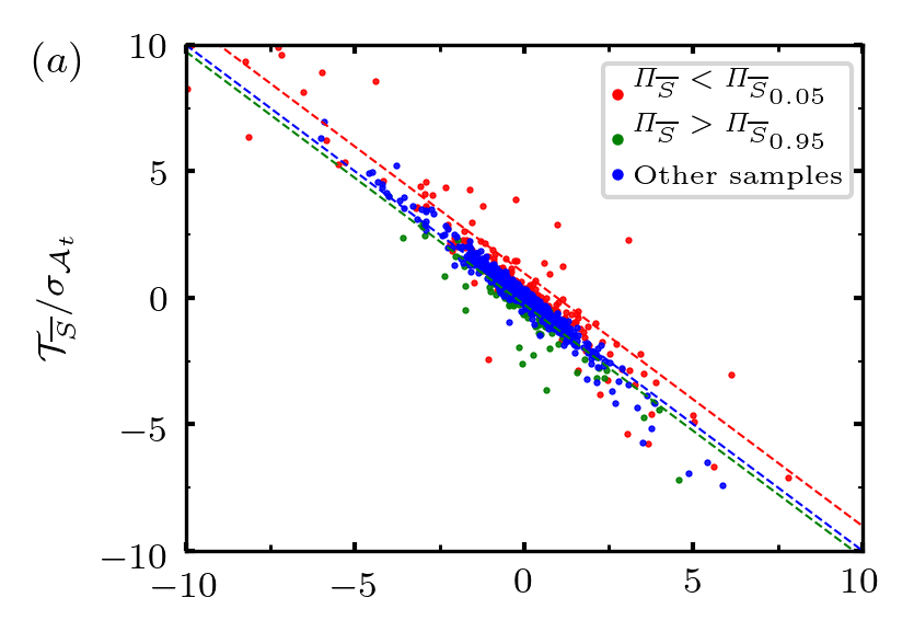
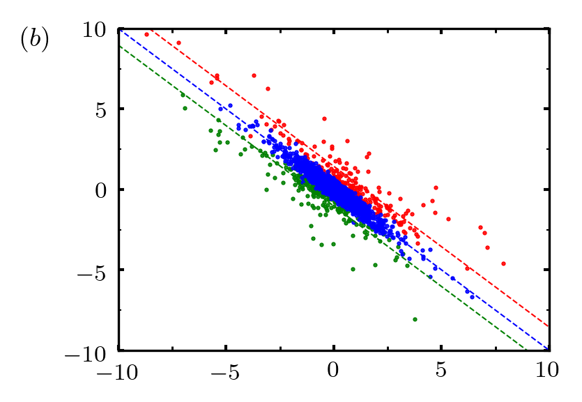
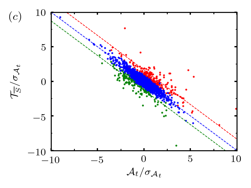
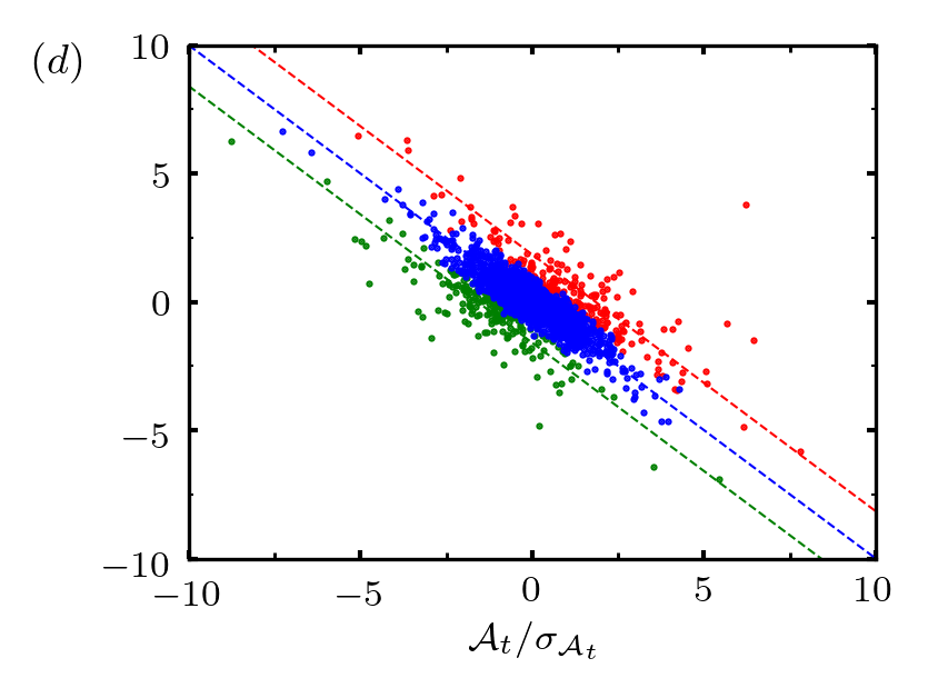
Figure 11: Scatter plots of $\mathcal{A}_{t}$ and $\mathcal{T}_{\overline{S}}$ at random orientations $\boldsymbol{r}$ normalised by $\sigma_{\mathcal{A}_{t}}$ and $\sigma_{\mathcal{T}_{\overline{S}}}$, their respective standard deviations. $\mathit{\Pi}_{\overline{S}_{0.05}}$ is the value of $\mathit{\Pi}_{\overline{S}}$ at the respective $r_{d}$ for which $5\%$ of the samples are more negative than $\mathit{\Pi}_{\overline{S}_{0.05}}$ and $\mathit{\Pi}_{\overline{S}_{0.95}}$ is the value of $\mathit{\Pi}_{\overline{S}}$ for which $95\%$ of the samples are more positive than $\mathit{\Pi}_{\overline{S}_{0.95}}$. The events $\mathit{\Pi}_{\overline{S}}<\mathit{\Pi}_{\overline{S}_{0.05}}$ and $\mathit{\Pi}_{\overline{S}}>\mathit{\Pi}_{\overline{S}_{0.95}}$ are marked in red and green respectively, while the remaining events are marked in blue. The red line marks $\mathcal{A}_{t}=-\mathcal{T}_{\overline{S}}-\langle\mathit{\Pi}_{\overline{S}}|\mathit{\Pi}_{\overline{S}}<\mathit{\Pi}_{\overline{S}_{0.05}}\rangle$, where $\langle\mathit{\Pi}_{\overline{S}}|\mathit{\Pi}_{\overline{S}}<\mathit{\Pi}_{\overline{S}_{0.05}}\rangle$ is the average value of $\mathit{\Pi}_{\overline{S}}$ conditioned on $\mathit{\Pi}_{\overline{S}}<\mathit{\Pi}_{\overline{S}_{0.05}}$. The green line marks $\mathcal{A}_{t}=-\mathcal{T}_{\overline{S}}-\langle\mathit{\Pi}_{\overline{S}}|\mathit{\Pi}_{\overline{S}}>\mathit{\Pi}_{\overline{S}_{0.95}}\rangle$ and the blue line marks $\mathcal{A}_{t}=-\mathcal{T}_{\overline{S}}$ (with all terms appropriately normalised with $\sigma_{\mathcal{A}_{t}}$ and $\sigma_{\mathcal{T}_{\overline{S}}}$). $r_{d}/\langle\lambda\rangle_{t}=(0.12,1.45,3.1,5.2)$ for $(a,b,c,d)$ and $\langle\Rey_{\lambda}\rangle_{t}=174$.

Following the question of local/instantaneous equilibrium, we now look for local/instantaneous sweeping. Figure 9 shows strong anti-correlation between $\mathcal{A}_{t}$ and $\mathcal{T}_{\overline{S}}$, increasingly so as $r_{d}$ decreases from large to small scales. Along with the fifth KHMH result at the end of the previous section (that the fluctuation magnitudes of $\mathcal{A}_{t}$ and $\mathcal{T}_{\overline{S}}$ become increasingly comparable as $r_{d}$ decreases), this anti-correlation tendency suggests a tendency towards $\mathcal{A}_{t}+\mathcal{T}_{\overline{S}}\approx 0$ at decreasing scales in agreement with the concept of two-point sweeping introduced in section 3.2. In other words, the sweeping of $|\delta\boldsymbol{u}|^{2}$ by the mainly large scale advection velocity $(\boldsymbol{u}^{+}+\boldsymbol{u}^{-})/2$ becomes increasingly strong with decreasing $r_{d}$. The scatter plots of $\mathcal{A}_{t}$ and $\mathcal{T}_{\overline{S}}$ in figure 11 make this local/instantaneous two-point sweeping tendency with decreasing $r_{d}$ very evident, but also indicate that significant values of positive or negative $\mathit{\Pi}_{\overline{S}}$ can cause increasing deviations from $\mathcal{A}_{t}+\mathcal{T}_{\overline{S}}\approx 0$ as $r_{d}$ increases. Note $\mathcal{A}_{t}+\mathcal{T}_{\overline{S}}+\mathit{\Pi}_{\overline{S}}\approx 0$ as indicated by the correlation coefficients in figure 9 between $\mathcal{A}_{t}+\mathcal{T}_{\overline{S}}$ and $-\mathit{\Pi}_{\overline{S}}$ (which exceed $0.95$ for $r_{d}\geq\langle\lambda\rangle_{t}$ at our Reynolds numbers) and by their overlapping fluctuation magnitudes in figure 6($a2$,$b2$). The fluctuations of $\mathit{\Pi}_{\overline{S}}$ increase in magnitude as $r_{d}$ increases and so do high values of $\mathit{\Pi}_{\overline{S}}$ too. The scatter plots in figure 11 highlight how the $5\%$ most negative $\mathit{\Pi}_{\overline{S}}$ events (values of $\mathit{\Pi}_{\overline{S}}$ for which the probability that $\mathit{\Pi}_{\overline{S}}$ is smaller than a negative value $\mathit{\Pi}_{\overline{S}_{0.05}}$ is 0.05) and the $5\%$ most positive $\mathit{\Pi}_{\overline{S}}$ events (values of $\mathit{\Pi}_{\overline{S}}$ for which the probability that $\mathit{\Pi}_{\overline{S}}$ is larger than a positive value $\mathit{\Pi}_{\overline{S}_{0.95}}$ is also 0.05) cause significant deviations from ”perfect sweeping” $\mathcal{A}_{t}=-\mathcal{T}_{\overline{S}}$, increasingly so for increasing $r_{d}$, in agreement with $\mathcal{A}_{t}+\mathcal{T}_{\overline{S}}+\mathit{\Pi}_{\overline{S}}\approx 0$.

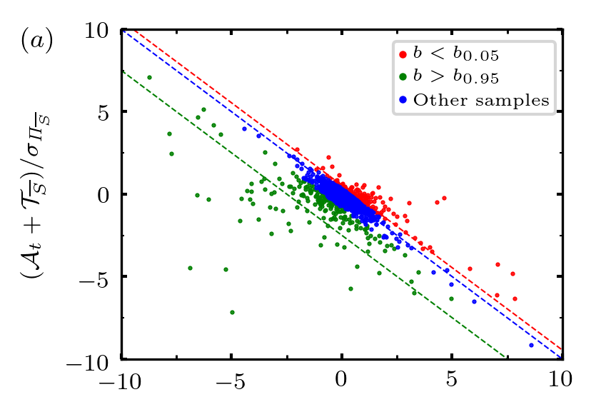
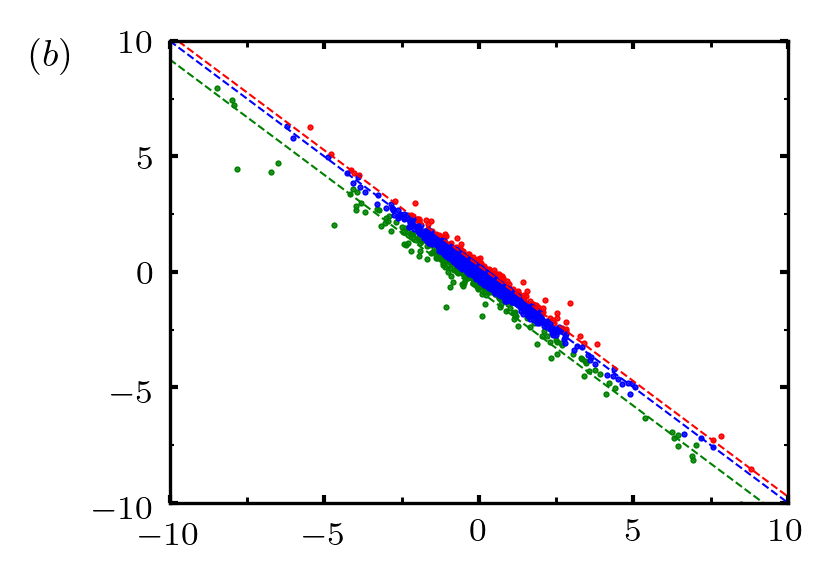
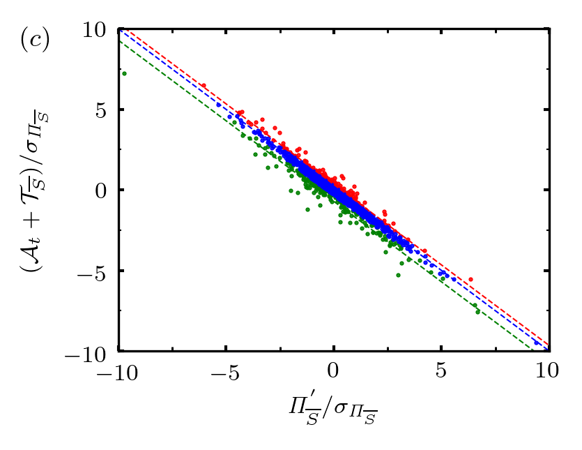
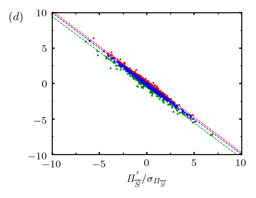
Figure 12: Scatter plots of $\mathcal{A}_{t}+\mathcal{T}_{\overline{S}}$ and $\mathit{\Pi}_{\overline{S}}^{{}^{\prime}}$ at random orientations $\boldsymbol{r}$. The residual $-b\equiv\mathcal{A}_{t}+\mathcal{T}_{\overline{S}}+\mathit{\Pi}_{\overline{S}}^{{}^{\prime}}$ and the values $b_{0.05}$ and $b_{0.95}$ are defined analogously as for $\mathit{\Pi}_{\overline{S}_{0.05}}$ and $\mathit{\Pi}_{\overline{S}_{0.95}}$ in the previous figure. The events $b<b_{0.05}$ and $b>b_{0.95}$ are marked in red and green respectively, while the remaining events are marked in blue. The red line marks $\mathcal{A}_{t}+\mathcal{T}_{\overline{S}}=-\mathit{\Pi}_{\overline{S}}^{{}^{\prime}}-\langle b|b<b_{0.05}\rangle$, the green line $\mathcal{A}_{t}+\mathcal{T}_{\overline{S}}=-\mathit{\Pi}_{\overline{S}}^{{}^{\prime}}-\langle b|b>b_{0.95}\rangle$ and the blue line $\mathcal{A}_{t}+\mathcal{T}_{\overline{S}}=-\mathit{\Pi}_{\overline{S}}^{{}^{\prime}}$ (with all terms appropriately normalised with $\sigma_{\mathit{\Pi}_{\overline{S}}}$). $r_{d}/\langle\lambda\rangle_{t}=(0.12,1.45,3.1,5.2)$ for $(a,b,c,d)$ and $\langle\Rey_{\lambda}\rangle_{t}=174$.

The scatter plots in figure 12 show that it is only in relatively rare circumstances that $\mathcal{A}_{t}+\mathcal{T}_{\overline{S}}+\mathit{\Pi}_{\overline{S}}\approx 0$ is significantly inaccurate for scales $r_{d}\geq\langle\lambda\rangle_{t}$. Similarly to NSD dynamics, $\mathcal{A}_{t}+\mathcal{T}_{\overline{S}}$ can be viewed as a Lagrangian time-rate of change of $|\delta\boldsymbol{u}|^{2}$ moving with $(\boldsymbol{u}^{+}+\boldsymbol{u}^{-})/2$. As more than average $|\delta\boldsymbol{u}|^{2}$ is cascaded from larger to smaller scales at a particular location $(\mathit{\Pi}_{\overline{S}}^{{}^{\prime}}<0)$, $\mathcal{A}_{t}+\mathcal{T}_{\overline{S}}$ increases; and as more than average $|\delta\boldsymbol{u}|^{2}$ is inverse cascaded from smaller to larger scales $(\mathit{\Pi}_{\overline{S}}^{{}^{\prime}}>0)$, $\mathcal{A}_{t}+\mathcal{T}_{\overline{S}}$ decreases. $\mathit{\Pi}_{\overline{S}}^{{}^{\prime}}$ is to a large extent determined by $\boldsymbol{a}_{\mathit{\Pi}_{\overline{S}}}$ which, as we show in appendix C, is a non-local function in space of the vortex stretching and compression dynamics determining the two-point vorticity difference $\delta\boldsymbol{\omega}$.

A fairly complete way to summarise the details of the balance $\mathcal{A}_{t}+\mathcal{T}_{\overline{S}}+\mathit{\Pi}_{\overline{S}}\approx 0$ at scales $r_{d}\geq\langle\lambda\rangle_{t}$ is by noting that, as $r_{d}$ decreases towards $\langle\lambda\rangle_{t}$, (i) the fluctuation magnitude of $\mathcal{T}_{\overline{S}}$ tends to become comparable to that of $\mathcal{A}_{t}$ while that of $\mathit{\Pi}_{\overline{S}}$ decreases by comparison, (ii) the correlation coefficient between $\mathcal{A}_{t}$ and $-\mathcal{T}_{\overline{S}}$ increases towards $0.9$, and also (iii) (not mentioned till now but evident in figure 9) the correlation coefficient between $\mathcal{A}_{t}$ and $-\mathit{\Pi}_{\overline{S}}$ decreases towards values below $0.2$.

4.2 Conditional correlations

At scales $r_{d}$ below $\langle\lambda\rangle_{t}$, the relation $\mathcal{A}_{t}+\mathcal{T}_{\overline{S}}+\mathit{\Pi}_{\overline{S}}\approx 0$ becomes less accurate as the correlation coefficient between $\mathcal{A}_{t}+\mathcal{T}_{\overline{S}}$ and $-\mathit{\Pi}_{\overline{S}}$ drops from $0.95$ to $0.7$ with decreasing $r_{d}$, reflecting the increase of correlation between $\mathcal{\epsilon}$ and $-\mathit{\Pi}_{\overline{S}}$ and the even higher increase towards values close to $0.5$ of the correlation coefficient between $\mathcal{D}$ and $\mathit{\Pi}_{\overline{S}}$. This increase of correlation appears to reflect the impact of relatively rare yet intense local/instantaneous occurances of interscale transfer rate as shown in figure 13 where we plot correlations conditional on relatively rare interscale events where the magnitudes of the spherically-averaged interscale transfer rates are higher than 95% of all interscale transfer rates of same sign (positive for backward and negative for forward transfer) in our overall spatio-temporal sample. This impact is highest at scales smaller than $\langle\lambda\rangle_{t}$ where the correlation coefficient conditioned on intense forward or backward interscale transfer rate events of $\pm\mathit{\Pi}_{\overline{S}}$ and either $\mathcal{\epsilon}$ or $\mathcal{D}$ can be as high as $0.7$ ($+\mathit{\Pi}_{\overline{S}}$ in the case of backward events and $-\mathit{\Pi}_{\overline{S}}$ in the case of forward events which causes significantly higher correlations between $\mathcal{A}_{t}+\mathcal{T}_{\overline{S}}$ and either $-\mathcal{\epsilon}$ or $\mathcal{D}$ in the case of backward events than in the case of forward events as seen in figure 13). However, the impact of such relatively rare events is also manifest at scales larger than $\langle\lambda\rangle_{t}$ (see figure 13) where the conditioned correlation coefficient is significantly higher than the unconditioned one in figure 9. Interestingly, conditioning on these relatively rare events does not change the correlation coefficients of $\mathcal{A}_{t}+\mathcal{T}_{\overline{S}}$ with $-\mathit{\Pi}_{\overline{S}}^{{}^{\prime}}$ except at scales $r_{d}$ smaller than $\langle\lambda\rangle_{t}$ where, consistently with the increased conditioned correlations between $-\mathit{\Pi}_{\overline{S}}$ and $\mathcal{D}$, they are smaller than the unconditional correlation coefficients of $\mathcal{A}_{t}+\mathcal{T}_{\overline{S}}$ with $-\mathit{\Pi}_{\overline{S}}^{{}^{\prime}}$, particularly at relatively rare forward interscale events where this conditional correlation drops to values close to $0.3$ at scales well below $\langle\lambda\rangle_{t}$.

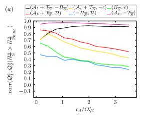
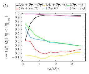
Figure 13: ($a$) Correlation coefficients among the $5\%$ strongest spherically averaged backward interscale transfer events $\mathit{\Pi}_{\overline{S}}^{a}>\mathit{\Pi}_{\overline{S}_{0.95}}^{a}$ for KHMH terms $(\mathcal{Q}_{1}^{a},\mathcal{Q}_{2}^{a})$ listed on top of the figure. ($b$) Correlation coefficients among the $5\%$ strongest spherically averaged forward interscale transfer events $\mathit{\Pi}_{\overline{S}}^{a}<\mathit{\Pi}_{\overline{S}_{0.05}}^{a}$ for KHMH terms $(\mathcal{Q}_{1}^{a},\mathcal{Q}_{2}^{a})$ listed on top of the figure. $\langle\Rey_{\lambda}\rangle_{t}=112$. (Corresponding plots for $\langle\Rey_{\lambda}\rangle_{t}=174$ are omitted because they are very similar.)

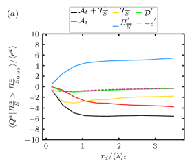
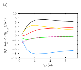
Figure 14: ($a$) Spatio-temporal averages of KHMH terms $\mathcal{Q}^{a}$ conditioned on the $5\%$ strongest spherically averaged backward ($a$) and forward $(b)$ interscale transfer events. The KHMH terms are listed above figure $(a)$ and $\langle\Rey_{\lambda}\rangle_{t}=112$.(Corresponding plots for $\langle\Rey_{\lambda}\rangle_{t}=174$ are omitted because they are very similar.)

Given that our relatively rare intense interscale transfer rates can be the seat of some correlation between $\mathit{\Pi}_{\overline{S}}$ and either $-\mathcal{\epsilon}$ or $\mathcal{D}$ particularly for $r_{d}<\langle\lambda\rangle_{t}$ , and given that $\mathcal{A}_{t}+\mathcal{T}_{\overline{S}}\approx 0$ is a good approximation at scales smaller than $\langle\lambda\rangle_{t}$, do we have approximate two-point sweeping and approximate equilibrium $\mathit{\Pi}_{\overline{S}}\approx\mathcal{D}$ if we condition on relatively rare forward or backward interscale transfer rate events? In fact the conditional correlations between $\mathcal{A}_{t}$ and $-\mathcal{T}_{\overline{S}}$ are very high (close to and above 0.95) at all scales (see figure 13), higher than the corresponding unconditional correlations. However, the conditional averages of $\mathcal{A}_{t}$ and $-\mathcal{T}_{\overline{S}}$ shown in figure 14 are also significantly different at all scales, implying that these strong conditional correlations do not actually amount to two-point sweeping at relatively rare forward and backward events. Furthermore, if we condition on high negative/positive values of $\mathit{\Pi}_{\overline{S}}$, the averages of both $\mathcal{A}_{t}$ and $\mathcal{T}_{\overline{S}}$ are positive/negative (figure 14), even though these conditional averages do tend to $0$ as $r_{d}$ tends to $0$. This has two implications. (i) It implies that, even though $\mathcal{A}_{t}$ and $-\mathcal{T}_{\overline{S}}$ are very well correlated at these relatively rare events, $\mathcal{A}_{t}+\mathcal{T}_{\overline{S}}$ fluctuates around a constant $C$ where $C>0$ if we condition the fluctuations on relatively rare negative $\mathit{\Pi}_{\overline{S}}$ but $C<0$ if we condition them on relatively rare positive $\mathit{\Pi}_{\overline{S}}$ ($C=0$ if we do not condition). This amounts to a systematic deviation on the average from two-point sweeping even though the strong correlation between the high magnitude fluctuations of $\mathcal{A}_{t}$ and $-\mathcal{T}_{\overline{S}}$ point at a tendency towards sweeping which is frustrated by the presence of the comparatively low non-zero local $\mathit{\Pi}_{\overline{S}}$. Given equation (33), the presence of this non-zero constant $C$ (clearly non-zero for all scales, and non-zero but tending towards zero as $r_{d}$ tends to $0$ well below $\langle\lambda\rangle_{t}$) means that the equilibrium $\mathit{\Pi}_{\overline{S}}\approx\mathcal{D}$ for scales smaller than $\langle\lambda\rangle_{t}$ does not hold either, even at scales smaller than $\langle\lambda\rangle_{t}$ where the conditional correlation between $\mathit{\Pi}_{\overline{S}}$ and $\mathcal{D}$ is significant. In fact, figure 14 shows that the conditional averages of $\mathit{\Pi}_{\overline{S}}^{\prime}$ are much larger than those of both $\mathcal{D}^{\prime}$ and $-\mathcal{\epsilon}^{{}^{\prime}}$; they are much closer to those of $\mathcal{A}_{t}+\mathcal{T}_{\overline{S}}$.

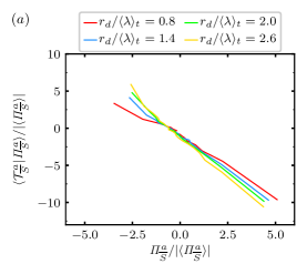
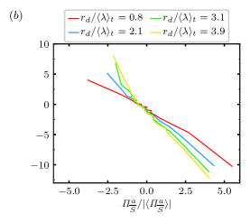
Figure 15: Spatio-temporal averages of $\mathcal{T}_{\overline{S}}^{a}$ across scales $r_{d}$ conditioned on $\mathit{\Pi}_{\overline{S}}^{a}$ being within a certain range of $\mathit{\Pi}_{\overline{S}}^{a}$ values and we consider $20$ such ranges of increasing values of $\mathit{\Pi}_{\overline{S}}^{a}$: the $5\%$ smallest/most negative $\mathit{\Pi}_{\overline{S}}^{a}$, the $5\%$ to $10\%$ smallest/most negative $\mathit{\Pi}_{\overline{S}}^{a}$ values and so on until the $5\%$ largest/most positive $\mathit{\Pi}_{\overline{S}}^{a}$ values. ($a$) $\langle\Rey\rangle_{t}=112$, ($b$) $\langle\Rey\rangle_{t}=174$.

(ii) The second implication of the conditional signs of $\mathcal{T}_{\overline{S}}$ is the existence of a relation between conditional average of solenoidal interspace transfer rate $\mathcal{T}_{\overline{S}}$ and the solenoidal interspace transfer rate $\mathit{\Pi}_{\overline{S}}$ on which the average is conditioned: when one is positive/negative the other is negative/positive, and we also find that their absolute magnitudes increase together (see figure 15). This is an observation which may prove important in the future for both subgrid scale modeling and the detailed study of the very smallest scales of turbulence fluctuations.

In conclusion, $\mathit{\Pi}_{\overline{S}}$ does not fluctuate with neither $-\mathcal{\epsilon}$ nor $\mathcal{D}$. Instead, $\mathit{\Pi}_{\overline{S}}$ and $\mathcal{A}_{t}+\mathcal{T}_{\overline{S}}$ fluctuate together at all scales, in particular scales larger than $\langle\lambda\rangle_{t}$, and even at relatively rare interscale transfer events. At scales smaller than $\langle\lambda\rangle_{t}$, we have a general tendency towards two-point sweeping if we do not condition on particular events. At our relatively rare interscale transfer events this correlation tendency (now conditional) is in fact amplified but there is nevertheless a systematic average deviation from two-point sweeping consistent with the absence of equilibrium $\mathit{\Pi}_{\overline{S}}\approx\mathcal{D}$ at these events. Finally, a relation exists between interspace and interscale transfer rates because the average interspace transfer rate conditioned on positive/negative values of interscale transfer rate is negative/positive. It must be stressed, however, that this relation does not imply an anticorrelation between interscale and interspace transport rates. The unconditioned correlation coefficients between $-\mathit{\Pi}_{\overline{S}}$ and $\mathcal{T}_{\overline{S}}$ are around $0.2$ (see figure 9), and we checked that this $0.2$ correlation does not change significantly if we condition on relatively rare intense occurances of interscale transfer rate.

5 Inhomogeneity contribution to interscale transfer

5.1 Average values and PDFs

The decomposition $\mathit{\Pi}=\mathit{\Pi}_{\overline{I}}+\mathit{\Pi}_{\overline{S}}$ helped us distinguish between the solenoidal vortex stretching/compression and the pressure-related aspects of the interscale transfer. As recently shown by Alves Portela et al. (2020), the interscale transfer rate $\mathit{\Pi}$ can also be decomposed in a way which brings out the fact that it has a direct inhomogeneity contribution to it. This last part of the present study is an examination of the decomposition introduced by Alves Portela et al. (2020) which is $\mathit{\Pi}=\mathit{\Pi}_{I}+\mathit{\Pi}_{H}$ where

$$\mathit{\Pi}_{I} =\ \ \frac{1}{2}\delta u_{i}\frac{\partial}{\partial x_{i}}(u_{k}^{+}u_{k}^{+}-u_{k}^{-}u_{k}^{-}),$$ (38)

$$\mathit{\Pi}_{H} =-2\delta u_{i}\frac{\partial}{\partial r_{i}}(u_{k}^{-}u_{k}^{+}).$$ (39)

$\mathit{\Pi}_{I}$ can be locally/instantaneously non-zero only in the presence of a local/instantaneous inhomogeneity. However, it averages to zero, i.e. $\langle\mathit{\Pi}_{I}\rangle=0$, in periodic/statistically homogeneous turbulence. Note that $\mathit{\Pi}=\mathit{\Pi}_{I}=\mathit{\Pi}_{H}=0$ at $\boldsymbol{r}=\boldsymbol{0}$. With $\boldsymbol{r}$-orientation-averaging, the decomposition $\mathit{\Pi}^{a}=\mathit{\Pi}_{I}^{a}+\mathit{\Pi}_{H}^{a}$ is unique in the sense that any potentially suitable (e.g. such that it equals $0$ at $\boldsymbol{r}=\boldsymbol{0}$) $\boldsymbol{x}$-gradient term added to $\mathit{\Pi}_{I}$ vanishes after $\boldsymbol{r}$-orientation-averaging (see Alves Portela et al. (2020)).

An equivalent expression for $\mathit{\Pi}_{I}$ which immediately reveals where the decomposition $\mathit{\Pi}=\mathit{\Pi}_{I}+\mathit{\Pi}_{H}$ comes from is $\mathit{\Pi}_{I}=\delta u_{i}\frac{\partial}{\partial r_{i}}(u_{k}^{+}u_{k}^{+}+u_{k}^{-}u_{k}^{-})$. Given that the total interscale transfer rate is $\mathit{\Pi}=\delta u_{i}\frac{\partial}{\partial r_{i}}(\delta u_{k}\delta u_{k})$, the $\mathit{\Pi}_{I}$ part of the interscale transfer concerns the transfered energy differences coming mostly from differences between velocity amplitudes, i.e. local/instantaneous inhomogeneities of “turbulence intensity” in the flow; the $\mathit{\Pi}_{H}$ part of the interscale transfer concerns transfered energy differences coming mostly from differences between velocity orientations. Consistently with its link to local/instantaneous non-homogeneity, $\mathit{\Pi}_{I}$ can be written in the form ((38)) making it clear that $\mathit{\Pi}_{I}$ is zero where and when fluctuating velocity magnitudes are locally uniform.

In comparing the decompositions $\mathit{\Pi}=\mathit{\Pi}_{\overline{S}}+\mathit{\Pi}_{\overline{I}}$ and $\mathit{\Pi}=\mathit{\Pi}_{I}+\mathit{\Pi}_{H}$, it is worth noting that $\mathit{\Pi}_{I}=\mathit{\Pi}_{I_{\overline{I}}}$ given that $\mathit{\Pi}_{I_{\overline{S}}}=0$ from its centroid gradient form (see equation (38)). It therefore follows that

$$\mathit{\Pi}_{\overline{S}} =\mathit{\Pi}_{H_{\overline{S}}},$$ (40)

$$\mathit{\Pi}_{\overline{I}} =\mathit{\Pi}_{I}+\mathit{\Pi}_{H_{\overline{I}}}.$$ (41)

The inhomogeneity-based interscale transfer rate influences only the irrotational part of the total interscale transfer rate whereas $\mathit{\Pi}_{H}$ influences both the irrotational and the solenoidal parts. As $\langle\mathit{\Pi}_{I}\rangle=0$ and $\langle\mathit{\Pi}_{\overline{I}}\rangle=0$, it follows that $\langle\mathit{\Pi}_{H_{\overline{I}}}\rangle=0$. More to the point, $\langle\mathit{\Pi}_{\overline{S}}\rangle$ equals $\langle\mathit{\Pi}_{H_{\overline{S}}}\rangle$ and so equation (32) reduces to

$$\langle\mathit{\Pi}\rangle=\langle\mathit{\Pi}_{H_{\overline{S}}}\rangle=\langle\mathcal{D}_{r,\nu}\rangle-\langle\mathcal{\epsilon}\rangle+\langle\mathcal{I}\rangle.$$ (42)

The part of the interscale transfer rate which is present in the average interscale transfer/cascade dynamics is in fact $\mathit{\Pi}_{H_{\overline{S}}}$.

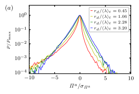
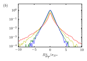
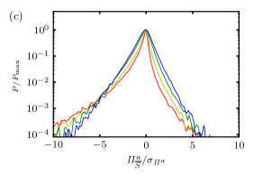
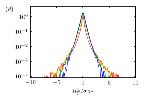
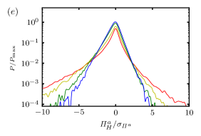
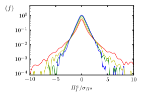
Figure 16: ($a,b,c,d,e,f$) PDFs of $\mathit{\Pi}$ decompositions $(\mathit{\Pi},\mathit{\Pi}_{H_{\overline{I}}},\mathit{\Pi}_{\overline{S}},\mathit{\Pi}_{\overline{I}},\mathit{\Pi}_{H},\mathit{\Pi}_{I})$ at $\langle\Rey_{\lambda}\rangle_{t}=112$. $\sigma_{\mathit{\Pi}^{a}}$ denotes the standard deviation of $\mathit{\Pi}^{a}$ and $P_{\text{max}}$ denotes the maximum value of the PDF of $\mathit{\Pi}^{a}$. The inhomogeneity and homogeneity interscale transfer rates $\mathit{\Pi}_{I}$ and $\mathit{\Pi}_{H}$ are defined in equations (38)-(39) and the irrotational part of the homogeneity interscale transfer rate $\mathit{\Pi}_{H_{\overline{I}}}$ in equation (41).

Given that the average interscale transfer is controlled by $\mathit{\Pi}_{H_{\overline{S}}}=\mathit{\Pi}_{\overline{S}}$, it is worth asking whether the well-known negative skewness of the PDF of $\mathit{\Pi}^{a}$ (e.g. see Yasuda & Vassilicos (2018) and references therein) is also present in the PDF of $\mathit{\Pi}_{\overline{S}}^{a}$ or/and whether it is spread across different terms of our two interscale transfer rate decompositions. In figure 16 we plot the PDFs of $\mathit{\Pi}^{a}$ and of the different $\boldsymbol{r}$-orientation-averaged terms in the decompositions of $\mathit{\Pi}$ that we use. It is clear that the PDFs of $\mathit{\Pi}$ and $\mathit{\Pi}_{\overline{S}}$ are nearly identical whilst the PDFs of $\mathit{\Pi}_{H}$ are different though also negatively skewed. The PDFs of $\mathit{\Pi}_{H_{\overline{I}}}$, $\mathit{\Pi}_{\overline{I}}$ and $\mathit{\Pi}_{I}$ are not significantly skewed. In figure 17 we plot the skewnes factors of the various interscale transfer terms as well as some other KHMH terms. The inhomogeneity interscale transfer $\mathit{\Pi}_{I}$ has close to zero skewness across scales. Both $\mathit{\Pi}_{\overline{S}}$ and $\mathit{\Pi}_{H}$ are negatively skewed, the former more so than the latter. Given equations (40)-(41) and $\mathit{\Pi}_{H}=\mathit{\Pi}_{\overline{S}}+\mathit{\Pi}_{H_{\overline{I}}}$, this difference in skewness factors is due to the irrotational part of $\mathit{\Pi}_{H}$ which is not significantly skewed and reduces the skewness of $\mathit{\Pi}_{H}$ relative to that of $\mathit{\Pi}_{\overline{S}}$. All in all, the skewness towards forward rather than inverse interscale transfers is present in its homogeneous and solenoidal components but is absent in its non-homogeneous and irrotational parts.

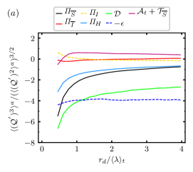
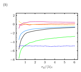
Figure 17: Skewness factors for KHMH terms $\mathcal{Q}$ listed on top of $(a)$: ($a$) $\langle\Rey_{\lambda}\rangle_{t}=112$, ($b$) $\langle\Rey_{\lambda}\rangle_{t}=174$.

Figure 17 also shows that $\mathcal{A}_{t}+\mathcal{T}_{\overline{S}}$ is slightly positively skewed with flatness factors of approximately $0.5$ at scales $r_{d}\geq\langle\lambda\rangle_{t}$ and close to 0 or below at scales below $\langle\lambda\rangle_{t}$. The skewness factor of $-\mathit{\Pi}_{\overline{S}}$ with which $\mathcal{A}_{t}+\mathcal{T}_{\overline{S}}$ is very well correlated (as we have seen in the previous section) is about the same at scales close to the integral scale but steadily increases to values well above $0.5$ as $r$ decreases, reaching nearly $6.0$ at scales close to $0.5\langle\lambda\rangle_{t}$. This is a concrete illustration of the fact already mentioned earlier in this paper that $\mathcal{A}_{t}+\mathcal{T}_{\overline{S}}\approx-\mathit{\Pi}_{\overline{S}}$ is a very good approximation for most locations and most times but not all. Given the very significantly increased correlation/anti-correlation of $\mathit{\Pi}_{\overline{S}}$ with both $\mathcal{D}$ and $\mathcal{\epsilon}$ at relatively intense forward/inverse interscale transfer events and with decreasing scale $r_{d}$, it is natural to expect the skewness factor of $\mathit{\Pi}_{\overline{S}}$ to veer towards the skewness factors of $\mathcal{D}$ and $-\mathcal{\epsilon}$ which, as can be seen in figure 17, are highly negative with values between $-3.0$ and $-7.0$.

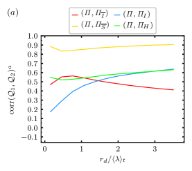
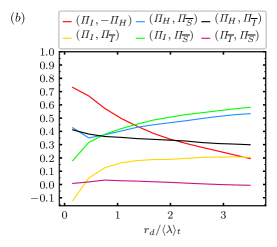
Figure 18: Correlation coefficients between various $\mathit{\Pi}$ decompositions $(\mathcal{Q}_{1},\mathcal{Q}_{2})$ listed on top of the figures at $\langle\Rey_{\lambda}\rangle_{t}=112$. (Corresponding plots for $\langle\Rey_{\lambda}\rangle_{t}=174$ are omitted because they are very similar.)

5.2 Correlations

We now consider the local/instantaneous relations between the various interscale transfer terms in terms of correlation coefficients plotted in figure 18$a$. First, note the very strong correlation between $\mathit{\Pi}$ and $\mathit{\Pi}_{\overline{S}}$ and the moderate correlation between $\mathit{\Pi}$ and $\mathit{\Pi}_{\overline{I}}$. Even though $\mathit{\Pi}$ and $\mathit{\Pi}_{\overline{S}}$ are highly correlated, we cannot ignore $\mathit{\Pi}_{\overline{I}}$ and cannot write $\mathit{\Pi}\approx\mathit{\Pi}_{\overline{S}}$. As seen earlier in the paper, we cannot ignore $\mathit{\Pi}_{\overline{I}}$ because it is the part of the interscale transfer which balances the pressure term, but we have also seen that the fluctuation magnitude of $\mathit{\Pi}_{\overline{S}}$ is significantly higher than the fluctuation magnitude of $\mathit{\Pi}_{\overline{I}}$. However, even if smaller, the fluctuation magnitude of $\mathit{\Pi}_{\overline{I}}$ is not neglible. There is no correlation between $\mathit{\Pi}_{\overline{S}}$ and $\mathit{\Pi}_{\overline{I}}$ (see figure 18b), and so $\mathit{\Pi}$ correlates with both $\mathit{\Pi}_{\overline{S}}$ (strongly) and $\mathit{\Pi}_{\overline{I}}$ (moderately) for different independent reasons. $\mathit{\Pi}$ feels the influence of solenoidal vortex stretching/compression via $\mathit{\Pi}_{\overline{S}}$ and the influence of pressure fluctuations via $\mathit{\Pi}_{\overline{I}}$, the former influencing $\mathit{\Pi}$ more than the latter.

Figure 18a also shows significantly smaller correlations between $\mathit{\Pi}$ and $\mathit{\Pi}_{H}$ than between $\mathit{\Pi}$ and $\mathit{\Pi}_{\overline{S}}$. This must be due to a decorrelating effect of $\mathit{\Pi}_{H_{\overline{I}}}$ as $\mathit{\Pi}_{H}=\mathit{\Pi}_{\overline{S}}+\mathit{\Pi}_{H_{\overline{I}}}$. The correlations between $\mathit{\Pi}$ and $\mathit{\Pi}_{I}$ are even smaller at the smaller scales but at integral size scales these correlations are equal to those between $\mathit{\Pi}$ and $\mathit{\Pi}_{H}$ (figure 18a).

Figure 18b reveals a strong anti-correlation between $\mathit{\Pi}_{I}$ and $\mathit{\Pi}_{H}$ at the small scales and a weak one at the large scales. As the scales decrease, the interscale transfers of fluctuating velocity differences caused by local/instantaneous non-homogeneities and the interscale transfers of fluctuating velocity differences caused by orientation differences get progressively more anti-correlated. This anti-correlation tendency results in $\mathit{\Pi}_{H}$ and $\mathit{\Pi}_{I}$ having larger fluctuation magnitudes than $\mathit{\Pi}$ at smaller scales, in particular scales smaller than $\langle\lambda\rangle_{t}$ (verified with our DNS data but not shown here for economy of space).

The other significant correlations revealed in figure 18b are those between $\mathit{\Pi}_{H}$ and $\mathit{\Pi}_{\overline{S}}$ and those between $\mathit{\Pi}_{I}$ and $\mathit{\Pi}_{\overline{S}}$, particularly as $r_{d}$ increases from around/below $\langle\lambda\rangle_{t}$ to the integral length scale. These correlations relate to the very stong correlations between $\mathit{\Pi}$ and $\mathit{\Pi}_{\overline{S}}$ but are weaker. One can imagine that $\mathit{\Pi}_{\overline{S}}$ correlates with $\mathit{\Pi}_{H}$ sometimes and with $\mathit{\Pi}_{I}$ some other times, but not too often with both given that $\mathit{\Pi}_{I}$ and $\mathit{\Pi}_{H}$ tend to be anti-correlated, and that this happens in a way subjected to a continuously strong correlation between $\mathit{\Pi}=\mathit{\Pi}_{H}+\mathit{\Pi}_{I}$ and $\mathit{\Pi}_{\overline{S}}$.

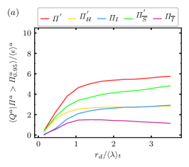
Figure 19: Average values of $\mathit{\Pi}$ decompositions conditioned on ($a$) intense backward events, ($b$) intense forward events at $\langle\Rey_{\lambda}\rangle_{t}=112$. The top of $(a)$ lists the $\mathit{\Pi}$ decompositions. (Corresponding plots for $\langle\Rey_{\lambda}\rangle_{t}=174$ are omitted because they are very similar.)

We finally consider in figure 19 the average contributions of the various $\mathit{\Pi}$-decomposition terms conditional on relatively rare intense $\mathit{\Pi}$-events. We calculate averages conditioned on $5\%$ most negative (forward transfer) $\mathit{\Pi}_{\overline{S}}$ events (values of $\mathit{\Pi}_{\overline{S}}$ for which the probability that $\mathit{\Pi}_{\overline{S}}$ is smaller than a negative value $\mathit{\Pi}_{\overline{S}_{0.05}}$ is 0.05) and on $5\%$ most positive $\mathit{\Pi}_{\overline{S}}$ (inverse transfer) events (values of $\mathit{\Pi}_{\overline{S}}$ for which the probability that $\mathit{\Pi}_{\overline{S}}$ is larger than a positive value $\mathit{\Pi}_{\overline{S}_{0.95}}$ is also 0.05). All these averages tend to $0$ as $r_{d}$ tends to $0$ below $\langle\lambda\rangle_{t}$. The largest such conditional averages are those of $\mathit{\Pi}^{\prime}$ followed by those of $\mathit{\Pi}_{\overline{S}}^{{}^{\prime}}$. This is the forward-skewed part of the interscale transfer (in terms of PDFs) and it is dominant at both forward and backward intense interscale transfer events. The weakest such conditional averages are those of $\mathit{\Pi}_{\overline{I}}$ for all $r_{d}$ and both forward and inverse extreme interscale transfer events. This is consistent with our observation in section 3.4 that the unconditional fluctuation magnitude of $\mathit{\Pi}_{\overline{I}}$ is smaller that the unconditional fluctuation magnitudes of $\mathit{\Pi}$ followed by those of $\mathit{\Pi}_{\overline{S}}$.

The most interesting point to notice in figure 19, however, is the difference between conditional averages of $\mathit{\Pi}_{H}^{{}^{\prime}}$ and $\mathit{\Pi}_{I}$ when conditioned on intense foward or intense inverse interscale transfer events. Whilst the conditional averages of these two quantities are about the same at intense inverse events, they differ substantially at forward transfer events where the conditional average of $-\mathit{\Pi}_{H}^{{}^{\prime}}$ is substantially higher that the conditional average of $-\mathit{\Pi}_{I}$ except close to the integral length-scale.

6 Conclusions

The balance between space-time-averaged interscale energy transfer rate on the one hand and space-time-averaged viscous diffusion, turbulence dissipation rate and power input on the other does not represent in any way the actual energy transfer dynamics in statistically stationary homogeneous/periodic turbulence. In this paper we have studied the fluctuations of two-point acceleration terms in the NSD equation and their relation to the various terms of the KHMH equation and we now give a summary of results in eleven points.

1. The various corresponding terms in the NSD and KHMH equations behave similarly relative to each other because the two-point velocity difference has a similar tendency of alignment with each one of the acceleration terms of the NSD equation.

2. The terms in the two-point energy balance which fluctuate with the highest magnitudes are $\mathcal{A}_{c}^{{}^{\prime}}$ followed closely by the time-derivative term $\mathcal{A}_{t}$ and the solenoidal interspace transfer rate $\mathcal{T}_{\overline{S}}$. The fluctuation intensity of $\mathcal{A}_{t}+\mathcal{T}_{\overline{S}}$ is much reduced by comparison to both these terms (two-point sweeping) and is comparable to the fluctuation intensity of the solenoidal interscale transfer rate. The solenoidal interscale transfer rate, which averages according to equation (32), does not fluctuate with viscous diffusion and/or turbulence dissipation with which it is negligibly correlated at scales larger than $\langle\lambda\rangle_{t}$ and rather weakly correlated at scales smaller than $\langle\lambda\rangle_{t}$. Its fluctuation magnitude is also significantly larger than that of $\mathcal{D}_{r,\nu}$, $-\mathcal{\epsilon}$ and $\mathcal{I}$ at all scales. Instead, the solenoidal interscale transfer rate fluctuates with $\mathcal{A}_{t}+\mathcal{T}_{\overline{S}}$ with which it is extremely well correlated at length scales larger than $\langle\lambda\rangle_{t}$ and very significantly correlated at length scales smaller than $\langle\lambda\rangle_{t}$.

3. In fact, for scales larger than $\langle\lambda\rangle_{t}$, the relation

$$\mathcal{A}_{t}+\mathcal{T}_{\overline{S}}+\mathit{\Pi}_{\overline{S}}^{{}^{\prime}} \approx 0,$$ (43)

is a good approximation for most times and most locations in the flow. $\mathcal{A}_{t}+\mathcal{T}_{\overline{S}}$ can be viewed as a Lagrangian time-rate of change of $|\delta\boldsymbol{u}|^{2}$ moving with $(\boldsymbol{u}^{+}+\boldsymbol{u}^{-})/2$. As more than average $|\delta\boldsymbol{u}|^{2}$ is cascaded from larger to smaller scales at a particular location $(\mathit{\Pi}_{\overline{S}}^{{}^{\prime}}<0)$, $\mathcal{A}_{t}+\mathcal{T}_{\overline{S}}$ increases; and as more than average $|\delta\boldsymbol{u}|^{2}$ is inverse cascaded from smaller to larger scales $(\mathit{\Pi}_{\overline{S}}^{{}^{\prime}}>0)$, $\mathcal{A}_{t}+\mathcal{T}_{\overline{S}}$ decreases. The relatively rare space-time events which do not comply with this relation are responsible for the different skewness factors of the PDFs of $\mathcal{A}_{t}+\mathcal{T}_{\overline{S}}$ (small, mostly positive, skewness factor) and of $\mathit{\Pi}_{\overline{S}}^{{}^{\prime}}$ (negative skewness factor reaching increasingly large negative values with decreasing scale).

4. As the length scale (i.e. two point separation length) decreases, the correlation between $\mathcal{A}_{t}$ and $-\mathcal{T}_{\overline{S}}$ increases and so do their fluctuation magnitudes relative to the fluctuation magnitude of $\mathit{\Pi}_{\overline{S}}^{{}^{\prime}}$ which reaches to be an order of magnitude smaller by comparison. In this limit, the correlation between $\mathcal{A}_{t}$ and $-\mathit{\Pi}_{\overline{S}}$ decreases. At length scales smaller than $\langle\lambda\rangle_{t}$ the correlation between $\mathcal{A}_{t}$ and $-\mathcal{T}_{\overline{S}}$ is extremely good indicating a tendency towards two-point sweeping. However, the correlation between $\mathcal{A}_{t}+\mathcal{T}_{\overline{S}}$ and $\mathit{\Pi}_{\overline{S}}^{{}^{\prime}}$ remains strong even if reduced from its near perfect values at length scales larger than $\langle\lambda\rangle_{t}$ and there remains a small difference of fluctuation magnitudes between $\mathcal{A}_{t}$ and $\mathcal{T}_{\overline{S}}$ which is mostly related to the small fluctuation magnitude of $\mathit{\Pi}_{\overline{S}}^{{}^{\prime}}$. At the other end of the length scale range, i.e. as the length scale tends towards the integral scale and larger, the fluctuation magnitudes of $\mathcal{T}_{\overline{S}}$ and $\mathit{\Pi}_{\overline{S}}^{{}^{\prime}}$ tend to become the same.

5. The irrotational part of the interscale transfer rate has zero spatio-temporal average but is exactly equal to the irrotational part of the interspace transfer rate and half the two-point pressure work term in the KHMH equation. A complete dynamic picture of the interscale transfer rate needs to also take this into account, even though the fluctuation magnitudes of these irrotational terms are smaller than the ones of the terms discussed in the previous paragraph. In fact, the exact relation $\mathit{\Pi}_{\overline{I}}=\mathcal{T}_{\overline{I}}=\frac{1}{2}\mathcal{T}_{p}$ explains the significant correlation between interscale transfer rate $\mathit{\Pi}$ and $\mathcal{T}_{p}$ reported by Yasuda & Vassilicos (2018).

6. The increase towards small correlations at length scales below $\langle\lambda\rangle_{t}$ between $\mathit{\Pi}_{\overline{S}}$ and both $\mathcal{D}_{r,\nu}$ and $-\mathcal{\epsilon}$ is accountable to the significant correlations between these terms at these viscous scales when conditioned on relatively rare intense $\mathit{\Pi}_{\overline{S}}$ events, both forward cascading events with negative values of $\mathit{\Pi}_{\overline{S}}$ of high magnitude and backward cascading events with positive values of $\mathit{\Pi}_{\overline{S}}$ of high magnitude. The choice of $\mathit{\Pi}_{\overline{S}}$ to identify relatively rare intense events is predicated on the fact that the PDFs of $\mathit{\Pi}_{\overline{S}}$ are negatively skewed similarly to the PDFs of $\mathit{\Pi}$, whereas the PDFs of $\mathit{\Pi}_{\overline{I}}$ are not. The solenoidal part of the interscale transfer rate derives from the integrated two-point vorticity equation and includes non-local vortex stretching/compression effects at all scales whereas the irrotational part of the interscale transfer rate derives from the integrated Poisson equation for two-point pressure fluctuations.

7. At these relatively rare intense interscale transfer rate events, the tendency for two-point sweeping may appear increased because of the extremely good conditional correlation between $\mathcal{A}_{t}$ and $-\mathcal{T}_{\overline{S}}$ at all length-scales, however $\mathcal{A}_{t}$ and $-\mathcal{T}_{\overline{S}}$ have also very significantly different average values given the high absolute values of $\mathit{\Pi}_{\overline{S}}$ at these relatively rare interscale transfer events. This implies that there is neither local/instantaneous sweeping nor local/instantaneous balance between $\mathit{\Pi}_{\overline{S}}$ and $\mathcal{D}$ or $\mathit{\Pi}_{\overline{S}}$ and $-\mathcal{\epsilon}$ at these relatively rare intense events, a conclusion confirmed by the observation that the conditional averages and the conditional fluctuation magnitudes of $\mathit{\Pi}_{\overline{S}}$ are much higher than those of $\mathcal{D}$ and $-\mathcal{\epsilon}$ in absolute values.

8. Another property of these relatively rare intense solenoidal interscale transfer rate events is that the conditional averages of solenoidal interscale and interspace transfer rates have opposite signs when sampling on these events. There is therefore a relation between them which may however be concealed by the fact that the fluctuation magnitudes of the interspace transport rate are higher than those of the interscale transfer rate.

9. We have also considered the decomposition into homogeneous and inhomogeneous interscale transfer rates recently introduced by Alves Portela et al. (2020) and have studied their fluctuations in statistically stationary homogeneous turulence. The PDFs of the homogeneous interscale transfer rate are skewed towards forward cascade events whereas the PDFs of the inhomogeneous interscale transfer rate are not significantly skewed. However, the skewness factors of the PDFs of the homogeneous interscale transfer rate are not as high as those of both the full and the solenoidal interscale transfer rates. Relating to this, $\mathit{\Pi}$ is highly correlated with $\mathit{\Pi}_{\overline{S}}$ more than with $\mathit{\Pi}_{\overline{I}}$, $\mathit{\Pi}_{H}$ and $\mathit{\Pi}_{I}$ with all of which $\mathit{\Pi}$ is, nevertheless, significantly correlated.

10. There is an increasing correlation between $\mathit{\Pi}_{I}$ and $-\mathit{\Pi}_{H}$ as the length-scale decreases, in particular below $\langle\lambda\rangle_{t}$ where it reaches values above 0.6. The interscale transfer of velocity difference energy caused by local inhomogeneities in fluctuating velocity magnitudes tends to cancel the interscale transfer of fluctuating velocity difference energy caused by misalignments between the two neighboring fluctuating velocities, in particular at length scales below $\langle\lambda\rangle_{t}$. As a result, the fluctuation magnitudes of $\mathit{\Pi}$ are smaller than those of both $\mathit{\Pi}_{I}$ and $-\mathit{\Pi}_{H}$.

11. Finally, the decomposition $\mathit{\Pi}=\mathit{\Pi}_{I}+\mathit{\Pi}_{H}$ can be used to physically distinguish between intense forward and intense inverse interscale transfer events. The averages of $\mathit{\Pi}_{H}^{{}^{\prime}}$ and $\mathit{\Pi}_{I}$ when conditioned on intense inverse interscale transfer events are about the same, but they differ substantially when conditioned on intense forward interscale transfer events where the conditional average of $-\mathit{\Pi}_{H}^{{}^{\prime}}$ is substantially higher that the conditional average of $-\mathit{\Pi}_{I}$ except close to the integral length-scale.

Future subgrid scale models for Large Eddy Simulations (LES) which are dynamic reduced order approaches to turbulent flows and their fluctuating large scales cannot rely on average cascade phenomenology describing spatio-temporal averages and should benefit from detailed descriptions of the fluctuating dynamics of interscale and interspace energy transfers such as the one presented in this paper. Whilst LES models based on local equilibrium such as the Smagorinsky model can reproduce structure function exponents and correlations between velocity increments and subgrid-scale energy transfers as shown by Linkmann et al. (2018), Dairay et al. (2017) have found that the Smagorinsky model is unable to ensure regularisation and is very sensitive to numerical errors. Furthermore, the recent review by Moser et al. (2021) makes it clear that the need for new subgrid models which can faithfully operate with coarse resolutions remains unanswered. The results in the present paper suggest that LES models based on local equilibrium (e.g. the Smagorinsky model) cannot be fully suitable for calculating fluctuations in subgrid stresses, a weakness which may become increasingly evident with coarser resolution. On the other hand, the good correlations between subgrid stresses from similarity models (Bardina et al., 1980; Cimarelli et al., 2019) and subgrid stresses from DNS suggest that these models might indeed approximate (unawarely) at least some of the cascade dynamics reported in this paper, for example the fact that $\mathcal{A}_{t}+\mathcal{T}_{\overline{S}}+\mathit{\Pi}_{\overline{S}}^{{}^{\prime}}\approx 0$ holds in most of the flow most of the time. This relation incorporates both forward and backward interscale transfers, yet a recent work by Vela-Martín (2022) argues that backscatter represents spatial fluxes and can therefore be ignored. It is not yet clear how such a claim can be understood in the context of the present paper’s results. Some new questions are therefore now raised concerning LES subgrid stess modeling which also need to be addressed in future work.

[Acknowledgements]We thank Professor S. Goto for allowing us to use his parallelised pseudo-spectral DNS code for periodic turbulence.

[Funding]HSL and JCV acknowledge support from EPSRC award number EP/L016230/1. JCV also acknowledges the Chair of Excellence CoPreFlo funded by I-SITE-ULNE (grant no. R-TALENT-19-001-VASSILICOS); MEL (grant no. CONVENTION-219-ESR-06) and Region Hauts de France (grant no. 20003862).

[Declaration of Interests]The authors report no conflict of interest.

Appendix A The Helmholtz decomposition in Fourier space

In this appendix we list the Helmholtz decomposition for periodic fields and note how this decomposition relates to the more general solution to the Helmholtz decomposition in the case of incompressible fields and fields which can be written as gradients of scalar fields.

Let $\boldsymbol{q}(\boldsymbol{x},t)$ be a periodic, twice continuously differentiable $3$D vector field with the Helmholtz decomposition $\boldsymbol{q}(\boldsymbol{x},t)=\boldsymbol{q}_{I}(\boldsymbol{x},t)+\boldsymbol{q}_{S}(\boldsymbol{x},t)$, where $\boldsymbol{q}_{I}(\boldsymbol{x},t)=-\nabla_{\boldsymbol{x}}\phi(\boldsymbol{x},t)$, $\boldsymbol{q}_{S}(\boldsymbol{x},t)=\nabla_{\boldsymbol{x}}\times\boldsymbol{B}(\boldsymbol{x},t)$. The scalar and vector potentials $\phi$ and $\boldsymbol{B}$ are unique within constants when $\nabla_{\boldsymbol{x}}\cdot\boldsymbol{q}$ and $\nabla_{\boldsymbol{x}}\times\boldsymbol{q}$ are known in the domain and $\boldsymbol{q}$ is known at the boundary (Bhatia et al., 2013). $\boldsymbol{q}(\boldsymbol{x},t)$ has the Fourier representation $\widehat{\boldsymbol{q}}(\boldsymbol{k},t)$, which can be decomposed into a component parallel to $\boldsymbol{k}$ (the longitudinal $\widehat{\boldsymbol{q}}^{L}$) and transverse to $\boldsymbol{k}$ (the transverse $\widehat{\boldsymbol{q}}^{T}$)

$$\widehat{\boldsymbol{q}}^{L}(\boldsymbol{k},t)=\frac{\boldsymbol{k}[\widehat{\boldsymbol{q}}(\boldsymbol{k},t)\cdot\boldsymbol{k}]}{k^{2}}\ ,\quad\widehat{\boldsymbol{q}}^{T}(\boldsymbol{k},t)=\widehat{\boldsymbol{q}}(\boldsymbol{k},t)-\widehat{\boldsymbol{q}}^{L}(\boldsymbol{k},t)\ .$$ (44)

It can be easily shown (see e.g. Stewart (2012)) that the irrotational part of $\boldsymbol{q}$ equals its longitudinal part $\boldsymbol{q}_{I}=\boldsymbol{q}^{L}$ and that the solenoidal part of $\boldsymbol{q}$ equals its transverse part $\boldsymbol{q}_{S}=\boldsymbol{q}^{T}$. Hence, (44) provides the Fourier representation of the Helmholtz decomposition of $\boldsymbol{q}$.

The Helmholtz decomposition can also be written for very general boundary conditions as (Sprössig, 2010)

$$\boldsymbol{q}_{IV}(\boldsymbol{x},t) =\frac{1}{4\upi}\int_{V}d\boldsymbol{y}\frac{\boldsymbol{x}-\boldsymbol{y}}{|\boldsymbol{x}-\boldsymbol{y}|^{3}}[\nabla_{\boldsymbol{y}}\cdot\boldsymbol{q}(\boldsymbol{y},t)],$$ (45)

$$\boldsymbol{q}_{IB}(\boldsymbol{x},t) =-\frac{1}{4\upi}\int_{S}dS_{\boldsymbol{y}}\frac{\boldsymbol{x}-\boldsymbol{y}}{|\boldsymbol{x}-\boldsymbol{y}|^{3}}[\widehat{\boldsymbol{n}}_{\boldsymbol{y}}\cdot\boldsymbol{q}(\boldsymbol{y},t)],$$ (46)

$$\boldsymbol{q}_{SV}(\boldsymbol{x},t) =-\frac{1}{4\upi}\int_{V}d\boldsymbol{y}\frac{\boldsymbol{x}-\boldsymbol{y}}{|\boldsymbol{x}-\boldsymbol{y}|^{3}}\times[\nabla_{\boldsymbol{y}}\times\boldsymbol{q}(\boldsymbol{y},t)],$$ (47)

$$\boldsymbol{q}_{SB}(\boldsymbol{x},t) =\frac{1}{4\upi}\int_{S}dS_{\boldsymbol{y}}\frac{\boldsymbol{x}-\boldsymbol{y}}{|\boldsymbol{x}-\boldsymbol{y}|^{3}}\times[\widehat{\boldsymbol{n}}_{\boldsymbol{y}}\times\boldsymbol{q}(\boldsymbol{y},t)].$$ (48)

where $\boldsymbol{q}_{I}=\boldsymbol{q}_{IV}+\boldsymbol{q}_{IB}$, $\boldsymbol{q}_{S}=\boldsymbol{q}_{SV}+\boldsymbol{q}_{SB}$ and $\widehat{\boldsymbol{n}}_{\boldsymbol{y}}$ denotes the unit surface normal at $\boldsymbol{y}$ and $dS_{\boldsymbol{y}}$ is the differential surface element at $\boldsymbol{y}$. For periodic vector fields $\boldsymbol{q}(\boldsymbol{x},t)$ that are incompressible or that can be written as the gradient of a scalar, this solution simplifies. In the case of a field $\boldsymbol{q}(\boldsymbol{x},t)$ which is incompressible $\nabla_{\boldsymbol{x}}\cdot\boldsymbol{q}(\boldsymbol{x},t)=0$, it can be shown that $\widehat{\boldsymbol{q}}(\boldsymbol{k},t)\cdot\boldsymbol{k}=0$ for every $\boldsymbol{k}$ (Pope, 2000). By inspection of (44), it is clear that this condition yields $\widehat{\boldsymbol{q}}^{L}(\boldsymbol{k},t)=0$ for every $\boldsymbol{k}$ such that $\widehat{\boldsymbol{q}}(\boldsymbol{k},t)=\widehat{\boldsymbol{q}}(\boldsymbol{k},t)^{T}$. By applying the Fourier transform to this relation and apply $\boldsymbol{q}^{T}(\boldsymbol{x},t)=\boldsymbol{q}_{S}(\boldsymbol{x},t)$ from above, we have that $\boldsymbol{q}(\boldsymbol{x},t)=\boldsymbol{q}_{S}(\boldsymbol{x},t)$ for incompressible periodic vector fields. In the case of $\boldsymbol{q}(\boldsymbol{x},t)=\nabla_{\boldsymbol{x}}\psi(\boldsymbol{x,t})$, where $\psi(\boldsymbol{x},t)$ is some scalar field, it can be shown that $\widehat{\boldsymbol{q}}(\boldsymbol{k},t)=i\boldsymbol{k}\widehat{\psi}(\boldsymbol{k},t)$ (Pope, 2000). If we insert this expression into the definition of $\widehat{\boldsymbol{q}}^{L}(\boldsymbol{k},t)$, it follows that $\widehat{\boldsymbol{q}}(\boldsymbol{k},t)=\widehat{\boldsymbol{q}}^{L}(\boldsymbol{k},t)$, which implies that $\boldsymbol{q}(\boldsymbol{x},t)=\boldsymbol{q}_{I}(\boldsymbol{x},t)$. If these properties are combined with equations (45)-(48), we have that a periodic incompressible vector field will have $\boldsymbol{q}_{IB}=\boldsymbol{q}_{IV}=0$ and that a periodic vector field that can be written as a gradient of a scalar field has $\boldsymbol{q}_{SB}=\boldsymbol{q}_{SV}=0$.

Appendix B Irrotational and solenoidal NSD tranport terms in Fourier space

We start this appendix with demonstrating that $\delta\boldsymbol{q}_{I}=\delta\boldsymbol{q}_{\overline{I}}$ and $\delta\boldsymbol{q}_{S}=\delta\boldsymbol{q}_{\overline{S}}$ for a periodic vector field $\boldsymbol{q}$ (see the second pararaph of section 3.3). The field $\boldsymbol{q}$ has the Fourier representation

$$\boldsymbol{q}(\boldsymbol{x},t)=\sum_{\boldsymbol{k}}\widehat{\boldsymbol{q}}(\boldsymbol{k},t)e^{i\boldsymbol{k}\cdot\boldsymbol{x}},$$ (49)

with the shifted fields

$$\boldsymbol{q}^{+}(\boldsymbol{x},\boldsymbol{r},t)=\boldsymbol{q}(\boldsymbol{x}+\boldsymbol{r}/2,t) =\sum_{\boldsymbol{k}}\widehat{\boldsymbol{q}}(\boldsymbol{k},t)e^{i\boldsymbol{k}\cdot(\boldsymbol{x}+\boldsymbol{r}/2)},$$ (50)

$$\boldsymbol{q}^{-}(\boldsymbol{x},\boldsymbol{r},t)=\boldsymbol{q}(\boldsymbol{x}-\boldsymbol{r}/2,t) =\sum_{\boldsymbol{k}}\widehat{\boldsymbol{q}}(\boldsymbol{k},t)e^{i\boldsymbol{k}\cdot(\boldsymbol{x}-\boldsymbol{r}/2)},$$ (51)

which have the Fourier coefficients

$$\widehat{\boldsymbol{q}^{+}}(\boldsymbol{k},\boldsymbol{r},t) =\widehat{\boldsymbol{q}}(\boldsymbol{k},t)e^{i\boldsymbol{k}\cdot\boldsymbol{r}/2},$$ (52)

$$\widehat{\boldsymbol{q}^{-}}(\boldsymbol{k},\boldsymbol{r},t) =\widehat{\boldsymbol{q}}(\boldsymbol{k},t)e^{-i\boldsymbol{k}\cdot\boldsymbol{r}/2}.$$ (53)

From the definition of the irrotational part of a vector field in (44), it follows

$$\delta\boldsymbol{q}_{I}(\boldsymbol{x},\boldsymbol{r},t) =\boldsymbol{q}_{I}^{+}(\boldsymbol{x},\boldsymbol{r},t)-\boldsymbol{q}_{I}^{-}(\boldsymbol{x},\boldsymbol{r},t),$$ (54)

$$=\sum_{\boldsymbol{k}}[\widehat{\boldsymbol{q}^{+}_{I}}(\boldsymbol{k},\boldsymbol{r},t)-\widehat{\boldsymbol{q}^{-}_{I}}(\boldsymbol{k},\boldsymbol{r},t)]e^{i\boldsymbol{k}\cdot\boldsymbol{x}},$$ (55)

$$=\sum_{\boldsymbol{k}}\frac{\boldsymbol{k}}{k^{2}}[\widehat{\boldsymbol{q}}(\boldsymbol{k},t)\cdot\boldsymbol{k}](e^{i\boldsymbol{k}\cdot\boldsymbol{r}/2}-e^{-i\boldsymbol{k}\cdot\boldsymbol{r}/2})e^{i\boldsymbol{k}\cdot\boldsymbol{x}},$$ (56)

$$=\sum_{\boldsymbol{k}}\frac{\boldsymbol{k}}{k^{2}}[\widehat{\boldsymbol{q}}(\boldsymbol{k},t)\cdot\boldsymbol{k}]2i\sin(\boldsymbol{k}\cdot\boldsymbol{r}/2)e^{i\boldsymbol{k}\cdot\boldsymbol{x}}.$$ (57)

Similarly, we can write

$$\delta\boldsymbol{q}(\boldsymbol{x},\boldsymbol{r},t) =\boldsymbol{q}^{+}(\boldsymbol{x},\boldsymbol{r},t)-\boldsymbol{q}^{-}(\boldsymbol{x},\boldsymbol{r},t),$$ (58)

$$=\sum_{\boldsymbol{k}}\widehat{\boldsymbol{q}}(\boldsymbol{k},t)2i\sin(\boldsymbol{k}\cdot\boldsymbol{r}/2)e^{i\boldsymbol{k}\cdot\boldsymbol{x}},$$ (59)

and then calculate its irrotational centroid part

$$\delta\boldsymbol{q}_{\overline{I}}(\boldsymbol{x},\boldsymbol{r},t)=\sum_{\boldsymbol{k}}\frac{\boldsymbol{k}}{k^{2}}[\widehat{\boldsymbol{q}}(\boldsymbol{k},t)\cdot\boldsymbol{k}]2i\sin(\boldsymbol{k}\cdot\boldsymbol{r}/2)e^{i\boldsymbol{k}\cdot\boldsymbol{x}},$$ (60)

which shows that $\delta\boldsymbol{q}_{I}(\boldsymbol{x},\boldsymbol{r},t)=\delta\boldsymbol{q}_{\overline{I}}(\boldsymbol{x},\boldsymbol{r},t)$. By combining this with $\delta\boldsymbol{q}=\delta\boldsymbol{q}_{I}+\delta\boldsymbol{q}_{S}=\delta\boldsymbol{q}_{\overline{I}}+\delta\boldsymbol{q}_{\overline{S}}$, we have also $\delta\boldsymbol{q}_{S}(\boldsymbol{x},\boldsymbol{r},t)=\delta\boldsymbol{q}_{\overline{S}}(\boldsymbol{x},\boldsymbol{r},t)$, which is what we wanted to show.

Next we demonstrate that $\boldsymbol{a}_{\mathit{\Pi}_{\overline{I}}}(\boldsymbol{k},\boldsymbol{r},t)=\boldsymbol{a}_{\mathcal{T}_{\overline{I}}}(\boldsymbol{x},\boldsymbol{r},t)$ in homogeneous/periodic turbulence. We list the following expressions for the vectors and tensors related to these two terms

$$\widehat{\delta u_{j}}(\boldsymbol{k},\boldsymbol{r},t) =2i\sin(\boldsymbol{k}\cdot\boldsymbol{r}/2)\widehat{u}_{j}(\boldsymbol{k},t),$$ (61)

$$\widehat{(u_{j}^{+}+u_{j}^{-})/2}(\boldsymbol{k},\boldsymbol{r},t) =\cos(\boldsymbol{k}\cdot\boldsymbol{r}/2)\widehat{u}_{j}(\boldsymbol{k},t),$$ (62)

$$\widehat{\frac{\partial\delta u_{i}}{\partial r_{j}}}(\boldsymbol{k},\boldsymbol{r},t) =ik_{j}\cos(\boldsymbol{k}\cdot\boldsymbol{r}/2)\widehat{u}_{i}(\boldsymbol{k},t),$$ (63)

$$\widehat{\frac{\partial\delta u_{i}}{\partial x_{j}}}(\boldsymbol{k},\boldsymbol{r},t) =-2k_{j}\sin(\boldsymbol{k}\cdot\boldsymbol{r}/2)\widehat{u}_{i}(\boldsymbol{k},t).$$ (64)

By use of these equations, we have that the Fourier coefficients of the transport terms read

$$\widehat{\boldsymbol{a}_{\mathcal{T}}}(\boldsymbol{k},\boldsymbol{r},t)=\sum_{\boldsymbol{k}=\boldsymbol{k}^{{}^{\prime}}+\boldsymbol{k}^{{}^{\prime\prime}}}-2\sin(\boldsymbol{k}^{{}^{\prime\prime}}\cdot\boldsymbol{r}/2)\cos(\boldsymbol{k}^{{}^{\prime}}\cdot\boldsymbol{r}/2)\widehat{u}_{j}(\boldsymbol{k}^{{}^{\prime}})k_{j}^{{}^{\prime\prime}}\widehat{\boldsymbol{u}}(\boldsymbol{k}^{{}^{\prime\prime}}),$$ (65)

$$\widehat{\boldsymbol{a}_{\mathit{\Pi}}}(\boldsymbol{k},\boldsymbol{r},t)=\sum_{\boldsymbol{k}=\boldsymbol{k}^{{}^{\prime}}+\boldsymbol{k}^{{}^{\prime\prime}}}-2\sin(\boldsymbol{k}^{{}^{\prime}}\cdot\boldsymbol{r}/2)\cos(\boldsymbol{k}^{{}^{\prime\prime}}\cdot\boldsymbol{r}/2)\widehat{u}_{j}(\boldsymbol{k}^{{}^{\prime}})k_{j}^{{}^{\prime\prime}}\widehat{\boldsymbol{u}}(\boldsymbol{k}^{{}^{\prime\prime}}).$$ (66)

Their irrotational parts are given per (44)

$$\widehat{\boldsymbol{a}_{\mathcal{T}_{\overline{I}}}}(\boldsymbol{k},\boldsymbol{r},t)=-\frac{\boldsymbol{k}}{k^{2}}\sum_{\boldsymbol{k}=\boldsymbol{k}^{{}^{\prime}}+\boldsymbol{k}^{{}^{\prime\prime}}}2\sin(\boldsymbol{k}^{{}^{\prime\prime}}\cdot\boldsymbol{r}/2)\cos(\boldsymbol{k}^{{}^{\prime}}\cdot\boldsymbol{r}/2)\widehat{u}_{j}(\boldsymbol{k}^{{}^{\prime}})k_{j}^{{}^{\prime\prime}}\widehat{u}_{l}(\boldsymbol{k}^{{}^{\prime\prime}})k^{{}^{\prime}}_{l},$$ (67)

$$\widehat{\boldsymbol{a}_{\mathit{\Pi}_{\overline{I}}}}(\boldsymbol{k},\boldsymbol{r},t)=-\frac{\boldsymbol{k}}{k^{2}}\sum_{\boldsymbol{k}=\boldsymbol{k}^{{}^{\prime}}+\boldsymbol{k}^{{}^{\prime\prime}}}2\sin(\boldsymbol{k}^{{}^{\prime}}\cdot\boldsymbol{r}/2)\cos(\boldsymbol{k}^{{}^{\prime\prime}}\cdot\boldsymbol{r}/2)\widehat{u}_{j}(\boldsymbol{k}^{{}^{\prime}})k_{j}^{{}^{\prime\prime}}\widehat{u}_{l}(\boldsymbol{k}^{{}^{\prime\prime}})k^{{}^{\prime}}_{l}.$$ (68)

If we employ the trigonometric identity $\sin x\cos y=\frac{1}{2}[\sin(x+y)+\sin(x-y)]$, we get

$$\widehat{\boldsymbol{a}_{\mathcal{T}_{\overline{I}}}}(\boldsymbol{k},\boldsymbol{r},t)=-\frac{\boldsymbol{k}}{k^{2}}\sum_{\boldsymbol{k}=\boldsymbol{k}^{{}^{\prime}}+\boldsymbol{k}^{{}^{\prime\prime}}}[\sin(\boldsymbol{k}\cdot\boldsymbol{r}/2)+\sin(\boldsymbol{k}^{{}^{\prime\prime}}\cdot\boldsymbol{r}/2-\boldsymbol{k}^{{}^{\prime}}\cdot\boldsymbol{r}/2)]\widehat{u}_{j}(\boldsymbol{k}^{{}^{\prime}})k_{j}^{{}^{\prime\prime}}\widehat{u}_{l}(\boldsymbol{k}^{{}^{\prime\prime}})k^{{}^{\prime}}_{l},$$ (69)

$$\widehat{\boldsymbol{a}_{\mathit{\Pi}_{\overline{I}}}}(\boldsymbol{k},\boldsymbol{r},t)=-\frac{\boldsymbol{k}}{k^{2}}\sum_{\boldsymbol{k}=\boldsymbol{k}^{{}^{\prime}}+\boldsymbol{k}^{{}^{\prime\prime}}}[\sin(\boldsymbol{k}\cdot\boldsymbol{r}/2)-\sin(\boldsymbol{k}^{{}^{\prime\prime}}\cdot\boldsymbol{r}/2-\boldsymbol{k}^{{}^{\prime}}\cdot\boldsymbol{r}/2)]\widehat{u}_{j}(\boldsymbol{k}^{{}^{\prime}})k_{j}^{{}^{\prime\prime}}\widehat{u}_{l}(\boldsymbol{k}^{{}^{\prime\prime}})k^{{}^{\prime}}_{l}.$$ (70)

Consider the term $\sin(\boldsymbol{k}^{{}^{\prime\prime}}\cdot\boldsymbol{r}/2-\boldsymbol{k}^{{}^{\prime}}\cdot\boldsymbol{r}/2)\widehat{u}_{j}(\boldsymbol{k}^{{}^{\prime}})k_{j}^{{}^{\prime\prime}}\widehat{u}_{l}(\boldsymbol{k}^{{}^{\prime\prime}})k^{{}^{\prime}}_{l}$. If one adds this term with the wavenumber triad $\boldsymbol{k}^{{}^{\prime}}=\boldsymbol{k}^{a}$ and $\boldsymbol{k}^{{}^{\prime\prime}}=\boldsymbol{k}^{b}\neq\boldsymbol{k}^{a}$ with the same term with the wavenumber triad $\boldsymbol{k}^{{}^{\prime}}=\boldsymbol{k}^{b}$ and $\boldsymbol{k}^{{}^{\prime\prime}}=\boldsymbol{k}^{a}$ the result is zero. Furthermore, in the case of $\boldsymbol{k}^{a}=\boldsymbol{k}^{b}$ this term is zero per incompressibility. This yields that this term does not contribute instantaneously in the above expressions such that we attain the final result (see section 3.3 and equation (26))

$$\widehat{\boldsymbol{a}_{\mathcal{T}_{\overline{I}}}}(\boldsymbol{k},\boldsymbol{r},t)=\widehat{\boldsymbol{a}_{\mathit{\Pi}_{\overline{I}}}}(\boldsymbol{k},\boldsymbol{r},t)=-\frac{\boldsymbol{k}}{k^{2}}\sin(\boldsymbol{k}\cdot\boldsymbol{r}/2)\sum_{\boldsymbol{k}=\boldsymbol{k}^{{}^{\prime}}+\boldsymbol{k}^{{}^{\prime\prime}}}\widehat{u}_{j}(\boldsymbol{k}^{{}^{\prime}})k_{j}^{{}^{\prime\prime}}\widehat{u}_{l}(\boldsymbol{k}^{{}^{\prime\prime}})k^{{}^{\prime}}_{l}.$$ (71)

Appendix C Irrotational and solenoidal dynamics in non-homogeneous turbulence

Here we deduce the generalised Tsinober equations and the irrotational and solenoidal NSD and KHMH equations applicable to non-homogeneous turbulence. Consider the twice continously differentiable vector field vector field $\boldsymbol{q}(\boldsymbol{x},t)$ defined on a domain $V\subseteq\mathbb{R}^{3}$ with the bounding surface $S$. This field can be uniquely decomposed into the irrotational and solenoidal vector fields

$$\boldsymbol{q}(\boldsymbol{x},t)=\boldsymbol{q}_{I}(\boldsymbol{x},t)+\boldsymbol{q}_{S}(\boldsymbol{x},t)=-\nabla_{\boldsymbol{x}}\boldsymbol{\phi}(\boldsymbol{x},t)+\nabla_{\boldsymbol{x}}\times\boldsymbol{B}(\boldsymbol{x},t),$$ (72)

The solution to this problem under very general conditions (Sprössig, 2010) is $\boldsymbol{q}_{I}=\boldsymbol{q}_{IV}+\boldsymbol{q}_{IB}$ and $\boldsymbol{q}_{S}=\boldsymbol{q}_{SV}+\boldsymbol{q}_{SB}$, where the solenoidal and irrotational volume and boundary terms are given in equations (45)-(48).

Consider an incompressible fluid that satisfies the incompressible vorticity equation

$$\nabla_{\boldsymbol{y}}\times\big{(}\frac{\partial\boldsymbol{u}}{\partial t}+\boldsymbol{u}\cdot\nabla_{\boldsymbol{y}}\boldsymbol{u}-\nu\nabla_{\boldsymbol{y}}^{2}\boldsymbol{u}-\boldsymbol{f}\big{)}=0.$$ (73)

By comparing this equation with (47), it is clear that the vorticity equation can be used to derive an evolution equation for the solenoidal volume parts of the NS terms. We can apply the following operator to this equation

$$-\frac{1}{4\upi}\int_{V}d\boldsymbol{y}\frac{\boldsymbol{x}-\boldsymbol{y}}{|\boldsymbol{x}-\boldsymbol{y}|^{3}}\times\Big{[}\nabla_{\boldsymbol{y}}\times\big{(}\frac{\partial\boldsymbol{u}}{\partial t}+(\boldsymbol{u}\cdot\nabla_{\boldsymbol{y}})\boldsymbol{u}-\nu\nabla_{\boldsymbol{y}}^{2}\boldsymbol{u}-\boldsymbol{f}\big{)}\Big{]}=0,$$ (74)

and use (47) to rewrite this equation as

$$(\frac{\partial\boldsymbol{u}}{\partial t})_{SV}+(\boldsymbol{u}\cdot\nabla_{\boldsymbol{x}}\boldsymbol{u})_{SV}=(\nu\nabla_{\boldsymbol{x}}^{2}\boldsymbol{u})_{SV}+\boldsymbol{f}_{SV}.$$ (75)

We can in a similar manner obtain the evolution equation for the irrotational volume NS terms from the Poisson equation for pressure

$$\frac{1}{4\upi}\int_{V}d\boldsymbol{y}\frac{\boldsymbol{x}-\boldsymbol{y}}{|\boldsymbol{x}-\boldsymbol{y}|^{3}}\Big{[}\nabla_{\boldsymbol{y}}\cdot\big{(}\boldsymbol{u}\cdot\nabla_{\boldsymbol{y}}\boldsymbol{u}+\frac{1}{\rho}\nabla_{\boldsymbol{y}}p-\boldsymbol{f}\big{)}\Big{]}=0,$$ (76)

which yields

$$(\boldsymbol{u}\cdot\nabla_{\boldsymbol{x}}\boldsymbol{u})_{IV}=(-\frac{1}{\rho}\nabla_{\boldsymbol{x}}p)_{IV}+\boldsymbol{f}_{IV},$$ (77)

The equations (75) and (77) state that in all incompressible turbulent flows the solenoidal accelerations from volume contributions balance with solenoidal forces from volume contributions and irrotational accelerations from volume contributions balance with irrotational forces from volume contributions. The former can be viewed as an integrated vorticity equation which dictates a part of the solenoidal NS dynamics, while the latter equation as an integrated pressure Poisson equation which dictates a part of the irrotational NS dynamics. Due to the non-local character of the solenoidal and irrotational volume terms, we reformulate these equations in terms of full NS term minus boundary terms. E.g., for the time-derivative $(\frac{\partial\boldsymbol{u}}{\partial t})_{SV}=\frac{\partial\boldsymbol{u}}{\partial t}-(\frac{\partial\boldsymbol{u}}{\partial t})_{IB}-(\frac{\partial\boldsymbol{u}}{\partial t})_{SB}$. The irrotational volume component (see (45)) involves an integral of the divergence of the respective term ($\nabla_{\boldsymbol{y}}\cdot\boldsymbol{q}(\boldsymbol{y})$). Thus, due to incompressibility, the time derivative and viscous terms have zero volume irrotational components, $(\frac{\partial\boldsymbol{u}}{\partial t})_{IV}=(\nu\nabla_{\boldsymbol{x}}^{2}\boldsymbol{u})_{IV}=0$. The solenoidal volume component (see (47)) involves an integral of the curl of the respective term, and as the curl of the pressure gradient equals zero, this term will have a zero solenoidal volume component, $(-\frac{1}{\rho}\nabla_{\boldsymbol{x}}p)_{SV}=0$. We rewrite the solenoidal volume terms in equation (75) in terms of combinations of full terms and boundary terms to obtain

$$\frac{\partial\boldsymbol{u}}{\partial t}+((\boldsymbol{u}\cdot\nabla_{\boldsymbol{x}})\boldsymbol{u})_{S}=\nu\nabla_{\boldsymbol{x}}^{2}\boldsymbol{u}+\boldsymbol{f}_{S}+\\ (\frac{\partial\boldsymbol{u}}{\partial t})_{IB}-(\nu\nabla_{\boldsymbol{x}}^{2}\boldsymbol{u})_{IB}+(\frac{\partial\boldsymbol{u}}{\partial t})_{SB}+((\boldsymbol{u}\cdot\nabla_{\boldsymbol{x}})\boldsymbol{u})_{SB}-(\nu\nabla_{\boldsymbol{x}}^{2}\boldsymbol{u})_{SB}-\boldsymbol{f}_{SB}\ ,$$ (78)

where the sum of the four rightmost terms on the RHS equals $(-\frac{1}{\rho}\nabla_{\boldsymbol{x}}p)_{SB}$ as the NS equations are satisfied at the boundary. By using this simplification and writing out all the boundary terms, we arrive at

$$\frac{\partial\boldsymbol{u}}{\partial t}+((\boldsymbol{u}\cdot\nabla_{\boldsymbol{x}})\boldsymbol{u})_{S}=\nu\nabla_{\boldsymbol{x}}^{2}\boldsymbol{u}+\boldsymbol{f}_{S}\\ -\frac{1}{4\upi}\int_{S}dS_{\boldsymbol{y}}\frac{\boldsymbol{x}-\boldsymbol{y}}{|\boldsymbol{x}-\boldsymbol{y}|^{3}}[\widehat{\boldsymbol{n}}_{\boldsymbol{y}}\cdot(\frac{\partial\boldsymbol{u}}{\partial t}-\nu\nabla_{\boldsymbol{y}}^{2}\boldsymbol{u})]-\frac{1}{4\upi}\int_{S}dS_{\boldsymbol{y}}\frac{\boldsymbol{x}-\boldsymbol{y}}{|\boldsymbol{x}-\boldsymbol{y}|^{3}}\times[\widehat{\boldsymbol{n}}_{\boldsymbol{y}}\times\nabla_{\boldsymbol{y}}\frac{1}{\rho}p].$$ (79)

By rewriting the irrotational volume components in equation (77) in terms of the full terms and the boundary terms, we have

$$((\boldsymbol{u}\cdot\nabla_{\boldsymbol{x}})\boldsymbol{u})_{I}=-\frac{1}{\rho}\nabla_{\boldsymbol{x}}p+\boldsymbol{f}_{I}+((\boldsymbol{u}\cdot\nabla_{\boldsymbol{x}})\boldsymbol{u})_{IB}-(-\frac{1}{\rho}\nabla_{\boldsymbol{x}}p)_{IB}-\boldsymbol{f}_{IB}-(-\frac{1}{\rho}\nabla_{\boldsymbol{x}}p)_{SB},$$ (80)

where the sum of the irrotational boundary terms equals $-(\frac{\partial\boldsymbol{u}}{\partial t})_{IB}+(\nu\nabla_{\boldsymbol{x}}^{2}\boldsymbol{u})_{IB}$ by the NS equations at the boundary. If we use this relation and write out all boundary terms, we have

$$((\boldsymbol{u}\cdot\nabla_{\boldsymbol{x}})\boldsymbol{u})_{I}=-\frac{1}{\rho}\nabla_{\boldsymbol{x}}p+\boldsymbol{f}_{I}\\ +\frac{1}{4\upi}\int_{S}dS_{\boldsymbol{y}}\frac{\boldsymbol{x}-\boldsymbol{y}}{|\boldsymbol{x}-\boldsymbol{y}|^{3}}[\widehat{\boldsymbol{n}}_{\boldsymbol{y}}\cdot(\frac{\partial\boldsymbol{u}}{\partial t}-\nu\nabla_{\boldsymbol{y}}^{2}\boldsymbol{u})]+\frac{1}{4\upi}\int_{S}dS_{\boldsymbol{y}}\frac{\boldsymbol{x}-\boldsymbol{y}}{|\boldsymbol{x}-\boldsymbol{y}|^{3}}\times[\widehat{\boldsymbol{n}}_{\boldsymbol{y}}\times\nabla_{\boldsymbol{y}}\frac{1}{\rho}p].$$ (81)

The equations (79) and (81) are generalisations of equations (8)-(9) for homogeneous/periodic turbulence and these equations are valid for all incompressible turbulent flows. The difference from homogeneous/periodic turbulence is the collection of boundary terms

$$\boldsymbol{R}(\boldsymbol{x},t) \equiv\frac{1}{4\upi}\int_{S}dS_{\boldsymbol{y}}\frac{\boldsymbol{x}-\boldsymbol{y}}{|\boldsymbol{x}-\boldsymbol{y}|^{3}}[\boldsymbol{n}_{\boldsymbol{y}}\cdot(\frac{\partial\boldsymbol{u}}{\partial t}-\nu\nabla_{\boldsymbol{y}}^{2}\boldsymbol{u})]+\frac{1}{4\upi}\int_{S}dS_{\boldsymbol{y}}\frac{\boldsymbol{x}-\boldsymbol{y}}{|\boldsymbol{x}-\boldsymbol{y}|^{3}}\times[\boldsymbol{n}_{\boldsymbol{y}}\times\nabla_{\boldsymbol{y}}\frac{1}{\rho}p],$$ (82)

$$=-(\boldsymbol{a}_{l})_{IB}+(\boldsymbol{a}_{\nu})_{IB}-(\boldsymbol{a}_{p})_{SB},$$ (83)

which yields the final expressions for the general irrotational and solenoidal NS equations

$$\frac{\partial\boldsymbol{u}}{\partial t}+((\boldsymbol{u}\cdot\nabla_{\boldsymbol{x}})\boldsymbol{u})_{S} =\nu\nabla_{\boldsymbol{x}}^{2}\boldsymbol{u}+\boldsymbol{f}_{S}-\boldsymbol{R}(\boldsymbol{x},t)$$ (84)

$$((\boldsymbol{u}\cdot\nabla_{\boldsymbol{x}})\boldsymbol{u})_{I} =-\frac{1}{\rho}\nabla_{\boldsymbol{x}}p+\boldsymbol{f}_{I}+\boldsymbol{R}(\boldsymbol{x},t)$$ (85)

In homogeneous/periodic turbulence all the boundary terms in $\boldsymbol{R}(\boldsymbol{x},t)$ equal zero individually (see the last parapgraph of A), such that we recover equations (8)-(9). In general, the boundary terms will be non-zero and differ in different flows. E.g., at a solid wall the boundary term from the time-derivative will vanish because of no-slip and the NS equations at the wall can be used to rewrite the boundary terms as a non-local function of the pressure gradient only.

The NSD irrotational and solenoidal equations in general turbulent flows are obtained by subtracting the solenoidal and irrotational NS equations (84)-(85) at $\boldsymbol{x}-\boldsymbol{r}/2$ from the same equations at $\boldsymbol{x}+\boldsymbol{r}/2$

$$\frac{\partial\delta\boldsymbol{u}}{\partial t}+\delta\boldsymbol{a}_{c_{S}} =\delta\boldsymbol{a}_{\nu}+\delta\boldsymbol{f}_{S}-\delta\boldsymbol{R},$$ (86)

$$\delta\boldsymbol{a}_{c_{I}} =-\frac{1}{\rho}\nabla_{\boldsymbol{x}}\delta p+\delta\boldsymbol{f}_{I}+\delta\boldsymbol{R},$$ (87)

The rephrasing of the irrotational and solenoidal NSD equations in terms of the interscale and interspace transport terms can also be performed for non-homogeneous turbulence. We derive the centroid irrotational and solenoidal NSD equations similarly as for the NS irrotational and solenoidal equations by starting with the NSD equation (13). This yields the equations

$$\delta\boldsymbol{a}_{l}+\boldsymbol{a}_{\mathcal{T}_{\overline{S}}}+\boldsymbol{a}_{\mathit{\Pi}_{\overline{S}}} =\delta\boldsymbol{a}_{\nu}+\delta\boldsymbol{f}_{\overline{S}}-\overline{\boldsymbol{R}},$$ (88)

$$\boldsymbol{a}_{\mathcal{T}_{\overline{I}}}+\boldsymbol{a}_{\mathit{\Pi}_{\overline{I}}} =\delta\boldsymbol{a}_{p}+\delta\boldsymbol{f}_{\overline{I}}+\overline{\boldsymbol{R}},$$ (89)

where

$$\overline{\boldsymbol{R}}(\boldsymbol{x},\boldsymbol{r},t) \equiv\frac{1}{4\upi}\int_{S}dS_{\boldsymbol{y}}\frac{\boldsymbol{x}-\boldsymbol{y}}{|\boldsymbol{x}-\boldsymbol{y}|^{3}}[\widehat{\boldsymbol{n}}_{\boldsymbol{y}}\cdot(\delta\boldsymbol{a}_{l}-\delta\boldsymbol{a}_{\nu})]-\frac{1}{4\upi}\int_{S}dS_{\boldsymbol{y}}\frac{\boldsymbol{x}-\boldsymbol{y}}{|\boldsymbol{x}-\boldsymbol{y}|^{3}}\times[\widehat{\boldsymbol{n}}_{\boldsymbol{y}}\times\delta\boldsymbol{a}_{p}],$$ (90)

$$=-(\delta\boldsymbol{a}_{l})_{IB}+(\delta\boldsymbol{a}_{\nu})_{IB}-(\delta\boldsymbol{a}_{p})_{SB}.$$ (91)

These boundary terms are individually equal to zero in homogeneous/periodic turbulence for the analogue reason as for the NS dynamics. Regarding the irrotational dynamics, in general, $\boldsymbol{a}_{\mathcal{T}_{\overline{I}}}\neq\boldsymbol{a}_{\mathit{\Pi}_{\overline{I}}}$, but the irrotational volume terms are always equal, $(\boldsymbol{a}_{\mathcal{T}})_{\overline{IV}}=(\boldsymbol{a}_{\mathit{\Pi}})_{\overline{IV}}$ from equation (45) and

$$\nabla_{\boldsymbol{x}}\cdot\boldsymbol{a}_{\mathit{\Pi}}=\nabla_{\boldsymbol{x}}\cdot\boldsymbol{a}_{\mathcal{T}}=\frac{1}{2}\big{(}\frac{\partial u_{k}^{+}}{\partial x^{+}_{i}}\frac{\partial u_{i}^{+}}{\partial x^{+}_{k}}-\frac{\partial u_{k}^{-}}{\partial x^{-}_{i}}\frac{\partial u_{i}^{-}}{\partial x^{-}_{k}}\big{)}.$$ (92)

The solenoidal interscale transfer term $\boldsymbol{a}_{\mathit{\Pi}_{\overline{S}}}$ in non-homogeneous turbulence can be written as

$$\boldsymbol{a}_{\mathit{\Pi}_{\overline{S}}}(\boldsymbol{x},\boldsymbol{r},t)=-\frac{1}{4\upi}\int_{V}d\boldsymbol{y}\frac{\boldsymbol{x}-\boldsymbol{y}}{|\boldsymbol{x}-\boldsymbol{y}|^{3}}\times[\nabla_{\boldsymbol{y}}\times\boldsymbol{a}_{\mathit{\Pi}}(\boldsymbol{y},\boldsymbol{r},t)]+\\ \frac{1}{4\upi}\int_{S}dS_{\boldsymbol{y}}\frac{\boldsymbol{x}-\boldsymbol{y}}{|\boldsymbol{x}-\boldsymbol{y}|^{3}}\times[\widehat{\boldsymbol{n}}_{\boldsymbol{y}}\times\boldsymbol{a}_{\mathit{\Pi}}(\boldsymbol{y},\boldsymbol{r},t)],$$ (93)

where the surface integral is of smaller order of magnitude than the volume integral away from boundaries and increasingly so with increasing $\langle\Rey_{\lambda}\rangle_{t}$ (verified in our periodic DNS). Hence, for a qualitative interpretation of $\boldsymbol{a}_{\mathit{\Pi}_{\overline{S}}}$, we consider $\boldsymbol{a}_{\mathit{\Pi}_{\overline{S}}}\approx\boldsymbol{a}_{\mathit{\Pi}_{\overline{SV}}}$ with

$$(\nabla_{\boldsymbol{x}}\times\boldsymbol{a}_{\mathit{\Pi}})_{i}=\delta u_{k}\frac{\partial\delta\omega_{i}}{\partial r_{k}}-\frac{\delta\omega_{k}}{2}\frac{s_{ij}^{+}+s_{ij}^{-}}{2}-\frac{\omega_{k}^{+}+\omega_{k}^{-}}{4}\delta s_{ij}+\frac{\epsilon_{ijk}}{2}[\frac{\partial u_{l}^{+}}{\partial x_{j}^{+}}\frac{\partial u_{k}^{-}}{\partial x_{l}^{-}}-\frac{\partial u_{l}^{-}}{\partial x_{j}^{-}}\frac{\partial u_{k}^{+}}{\partial x_{l}^{+}}],$$ (94)

where $s_{ij}$ is the strain-rate tensor and $\epsilon_{ijk}$ is the Levi-Civita tensor. This set of terms constitutes a part of the non-linear term in the the evolution equation for the vorticity difference $\delta\boldsymbol{\omega}(\boldsymbol{x},\boldsymbol{r},t)$, i.e. vorticity at scales $|\boldsymbol{r}|$ and smaller, as $\nabla_{\boldsymbol{x}}\times\delta\boldsymbol{a}_{c}=\nabla_{\boldsymbol{x}}\times(\boldsymbol{a}_{\mathit{\Pi}}+\boldsymbol{a}_{\mathcal{T}})$. If one contracts (94) with $2\delta\boldsymbol{\omega}$, the RHS corresponds to non-linear terms which determine the evolution of the enstrophy $|\delta\boldsymbol{\omega}|^{2}$ at scales smaller or comparable to $|\boldsymbol{r}|$. We interpret the first term on the RHS in (94) as vorticity interscale transfer. By the connection to $|\delta\boldsymbol{\omega}|^{2}$, we interpret the second and third terms as related to the enstrophy production/destruction at scales smaller or comparable to $|\boldsymbol{r}|$ due to interactions between the vorticity and strain fields. These three terms justify the interpretation of $\boldsymbol{a}_{\mathit{\Pi}_{\overline{S}}}$ being related non-locally in space to vortex stretching and compression dynamics. The last term in (94) appears in $\nabla_{\boldsymbol{x}}\times\boldsymbol{a}_{\mathcal{T}_{\overline{SV}}}$ with a negative sign such that these terms cancel.

The exact solenoidal and irrotational KHMH equations follows from contracting equations (88)-(89) with $2\delta\boldsymbol{u}$

$$\mathcal{A}_{t}+\mathcal{T}_{\overline{S}}+\mathit{\Pi}_{\overline{S}} =\mathcal{D}_{r,\nu}+\mathcal{D}_{X,\nu}-\mathcal{\epsilon}+I_{\overline{S}}-2\delta\boldsymbol{u}\cdot\overline{\boldsymbol{R}},$$ (95)

$$\mathcal{T}_{\overline{I}}+\mathit{\Pi}_{\overline{I}} =\mathcal{T}_{p}+I_{\overline{I}}+2\delta\boldsymbol{u}\cdot\overline{\boldsymbol{R}},$$ (96)

where $\mathcal{T}_{\overline{IV}}=\mathit{\Pi}_{\overline{IV}}$. This shows that the solenoidal and irrotational KHMH equations can be extended to non-homogeneous turbulence. In contrast to homogeneous/periodic turbulence, in general boundary terms couple the irrotational and solenoidal dynamics.

References

- Alves Portela et al. (2020) Alves Portela, F., Papadakis, G. & Vassilicos, J. C. 2020 The role of coherent structures and inhomogeneity in near-field interscale turbulent energy transfers. J. Fluid Mech. 896, A16.
- Bardina et al. (1980) Bardina, J., Ferziger, J. & Reynolds, W. 1980 Improved subgrid-scale models for large-eddy simulation. In 13th Fluid and Plasma Dynamics Conference. AIAA.
- Bhatia et al. (2013) Bhatia, H., Norgard, G., Pascucci, V. & Bremer, P. 2013 The Helmholtz-Hodge decomposition—a survey. IEEE Trans. Vis. Comput. Graph. 19 (8), 1386–1404.
- Chen et al. (2021) Chen, J. G., Cuvier, C., Foucaut, J.-M., Ostovan, Y. & Vassilicos, J. C. 2021 A turbulence dissipation inhomogeneity scaling in the wake of two side-by-side square prisms. J. Fluid Mech. 924, A4.
- Chen & Vassilicos (2022) Chen, J. G. & Vassilicos, J. C. 2022 Scalings of scale-by-scale turbulence energy in non-homogeneous turbulence. J. Fluid Mech. 938, A7.
- Chevillard et al. (2005) Chevillard, L., Roux, S. G., Lévêque, E., Mordant, N., Pinton, J.-F. & Arnéodo, A. 2005 Intermittency of velocity time increments in turbulence. Phys. Rev. Lett. 95 (6), 64501.
- Cimarelli et al. (2019) Cimarelli, A., Abbà, A. & Germano, M. 2019 General formalism for a reduced description and modelling of momentum and energy transfer in turbulence. J. Fluid Mech. 866, 865–896.
- Dairay et al. (2017) Dairay, Thibault, Lamballais, Eric, Laizet, Sylvain & Vassilicos, John Christos 2017 Numerical dissipation vs. subgrid-scale modelling for large eddy simulation. J. Comput. Phys. 337, 252–274.
- Frisch (1995) Frisch, U. 1995 Turbulence: the legacy of A. N. Kolmogorov. Cambridge University Press.
- Galanti & Tsinober (2000) Galanti, B. & Tsinober, A. 2000 Self-amplification of the field of velocity derivatives in quasi-isotropic turbulence. Phys. Fluids 12 (12), 3097–3099.
- Goto & Vassilicos (2016) Goto, S. & Vassilicos, J. C. 2016 Unsteady turbulence cascades. Phys. Rev. E 94 (5), 53108.
- Gulitski et al. (2007) Gulitski, G., Kholmyansky, M., Kinzelbach, W., Lüthi, B., Tsinober, A. & Yorish, S. 2007 Velocity and temperature derivatives in high-Reynolds-number turbulent flows in the atmospheric surface layer. Part 2. Accelerations and related matters. J. Fluid Mech. 589, 83–102.
- Helmholtz (1867) Helmholtz, H. 1867 On Integrals of the hydrodynamical equations, which express vortex-motion. Lond. Edinb. Dubl. Phil. Mag. 33 (226), 485–512.
- Hill (2002) Hill, R. J. 2002 Exact second-order structure-function relationships. J. Fluid Mech. 468, 317–326.
- Hill & Thoroddsen (1997) Hill, R. J. & Thoroddsen, S. T. 1997 Experimental evaluation of acceleration correlations for locally isotropic turbulence. Phys. Rev. E 55 (2), 1600–1606.
- Kolmogorov (1941a) Kolmogorov, A. N. 1941a Dissipation of energy in locally isotropic turbulence. Dokl. Akad. Nauk SSSR 32, 16–18.
- Kolmogorov (1941b) Kolmogorov, A. N. 1941b On the degeneration of isotropic turbulence in an incompressible viscous fluid. Dokl. Akad. Nauk SSSR 31, 538–540.
- Kolmogorov (1941c) Kolmogorov, A. N. 1941c The local structure of turbulence in incompressible viscous fluid for very large Reynolds numbers. Dokl. Akad. Nauk SSSR 30, 301–305.
- Leschziner (2016) Leschziner, M. 2016 Statistical turbulence modelling for fluid dynamics, demystified : an introductory text for graduate engineering students. Imperial College Press.
- Linkmann (2018) Linkmann, Moritz 2018 Effects of helicity on dissipation in homogeneous box turbulence. J. Fluid Mech. 856, 79–102.
- Linkmann et al. (2018) Linkmann, Moritz, Buzzicotti, Michele & Biferale, Luca 2018 Multi-scale properties of large eddy simulations: correlations between resolved-scale velocity-field increments and subgrid-scale quantities. J. Turb. 19 (6), 493–527.
- Linkmann & Morozov (2015) Linkmann, Moritz F & Morozov, Alexander 2015 Sudden relaminarization and lifetimes in forced isotropic turbulence. Phys. Rev. Lett. 115 (13), 134502.
- McComb et al. (2015a) McComb, W D, Berera, A, Yoffe, S R & Linkmann, M F 2015a Energy transfer and dissipation in forced isotropic turbulence. Phys. Rev. E 91 (4), 43013.
- McComb et al. (2015b) McComb, W. D., Linkmann, M. F., Berera, A., Yoffe, S. R. & Jankauskas, B. 2015b Self-organization and transition to turbulence in isotropic fluid motion driven by negative damping at low wavenumbers. J. Phys. A 48 (25), 25FT01.
- Monin et al. (1975) Monin, A. S, Yaglom, A. M. & Lumley, J. L. 1975 Statistical fluid mechanics, , vol. 2. M.I.T. Press.
- Moser et al. (2021) Moser, Robert D, Haering, Sigfried W & Yalla, Gopal R 2021 Statistical properties of subgrid-scale turbulence models. Annu. Rev. Fluid Mech. 53 (1), 255–286.
- Patterson & Orszag (1971) Patterson, G. S. & Orszag, S. A. 1971 Spectral calculations of isotropic turbulence: efficient removal of aliasing interactions. Phys. Fluids 14 (11), 2538–2541.
- Podvigina & Pouquet (1994) Podvigina, O. & Pouquet, A. 1994 On the non-linear stability of the 1:1:1 ABC flow. Physica D 75 (4), 471–508.
- Pope (2000) Pope, S. B. 2000 Turbulent flows. Cambridge University Press.
- Sagaut (2000) Sagaut, P. 2000 Large eddy simulation for incompressible flows: an introduction, 1st edn. Springer.
- Sprössig (2010) Sprössig, W. 2010 On Helmholtz decompositions and their generalizations—an overview. Math. Methods Appl. Sci. 33 (4), 374–383.
- Sreenivasan & Antonia (1997) Sreenivasan, K. R. & Antonia, R. A. 1997 The phenomenology of small-scale turbulence. Annu. Rev. Fluid Mech. 29 (1), 435–472.
- Steiros (2022) Steiros, K. 2022 Balanced nonstationary turbulence. Phys. Rev. E 105 (3), 35109.
- Stewart (2012) Stewart, A. M. 2012 Longitudinal and transverse components of a vector field. Sri Lankan J. Phys. 12 (0), 33.
- Tang et al. (2022) Tang, S L, Antonia, R A & Djenidi, L 2022 Transport equations for the normalized nth-order moments of velocity derivatives in grid turbulence. J. Fluid Mech. 930, A31.
- Tennekes (1975) Tennekes, H. 1975 Eulerian and lagrangian time microscales in isotropic turbulence. J. Fluid Mech. 67 (3), 561–567.
- Tsinober et al. (2001) Tsinober, A., Vedula, P. & Yeung, P. K. 2001 Random Taylor hypothesis and the behavior of local and convective accelerations in asotrophic turbulence. Phys. Fluids 13 (7), 1974–1984.
- Vassilicos (2015) Vassilicos, J. C. 2015 Dissipation in turbulent flows. Annu. Rev. Fluid Mech. 47 (1), 95–114.
- Vedula & Yeung (1999) Vedula, P. & Yeung, P. K. 1999 Similarity scaling of acceleration and pressure statistics in numerical simulations of isotropic turbulence. Phys. Fluids 11 (5), 1208–1220.
- Vela-Martín (2022) Vela-Martín, Alberto 2022 Subgrid-scale models of isotropic turbulence need not produce energy backscatter. J. Fluid Mech. 937, A14.
- Xu et al. (2007) Xu, H., Ouellette, N. T., Vincenzi, D. & Bodenschatz, E. 2007 Acceleration correlations and pressure structure functions in high-Reynolds number turbulence. Phys. Rev. Lett. 99 (20), 204501.
- Yasuda & Vassilicos (2018) Yasuda, T. & Vassilicos, J. C. 2018 Spatio-temporal intermittency of the turbulent energy cascade. J. Fluid Mech. 853, 235–252.
- Yeung et al. (2006) Yeung, P. K., Pope, S. B., Lamorgese, A. G. & Donzis, D. A. 2006 Acceleration and dissipation statistics of numerically simulated isotropic turbulence. Phys. Fluids 18 (6), 65103.