Higher structures in matrix product states

Abstract

For a parameterized family of invertible states (short-range-entangled states) in $(1+1)$ dimensions, we discuss a generalization of the Berry phase. Using translationally-invariant, infinite matrix product states (MPSs), we introduce a gerbe structure, a higher generalization of complex line bundles, as an underlying mathematical structure describing topological properties of a parameterized family of matrix product states. We also introduce a ”triple inner product” for three matrix product states, which allows us to extract a topological invariant, the Dixmier-Douady class over the parameter space.

I Introduction

I.1 The Berry Phase and Its Higher Generalization

Quantum mechanical phase degrees of freedom are known to have an interesting interplay with topology [1, 2]. A canonical example is the Dirac monopole where the presence of a magnetic monopole prevents quantum mechanical wave functions from being defined uniquely over the entire space. Instead, wave functions can be defined by introducing multiple patches, and at the intersection of two patches, wave functions from different patches are related by a transition function [3]. The (large) gauge invariance results in the quantization of magnetic charges in units of the inverse of the fundamental charge. A magnetic monopole also arises in the context of the Berry phase, where a diabolic point of the Hamiltonian plays the role of the Dirac monopole of the Berry connection in a parameterized quantum system where the wave function $|\psi(x)\rangle$ depends smoothly on some adiabatic parameter(s) $x$ taken from a parameter space $X$. The mathematical structure underlying these situations is a principle U(1) bundle over the parameter space $X$. Such bundles are characterized and classified by a topological invariant, the first Chern class taking its value in the second cohomology group of $X$, $\mathrm{H}^{2}(X;\mathbb{Z})$.

The Berry phase also plays an important role in topological phenomena in many-body quantum physics such as quantum Hall states and Chern insulators [4, 5] and the Thouless pump [6]. An important class of topological states is the so-called invertible states (short-range-entangled states) that are realized as a unique ground state of a gapped Hamiltonian. Invertible states can be protected by symmetry from being topologically trivial (symmetry-protected topological (SPT) phases), as known in topological insulators and the Haldane spin chain [7, 8, 9, 10]. Symmetry-protected (and often discrete) Berry phases are important in characterizing these phases. There are however many-body systems where the regular notion of the Berry phase fails to capture topological properties. In recent years, a family of invertible states that depends on some parameter $x\in X$ has been discussed [12, 13, 14, 15, 16, 17, 18, 19, 20]. Such a family can be topologically non-trivial and can be considered as a generalization of the Thouless pump. It can also be considered as a generalization of regular gapped phases (SPT phases) where the parameter space is a single point. For example, it is known that there is a nontrivial family of $(d+1)$-dimensional systems with $\mathrm{U}(1)$ symmetry parameterized over $S^{d}$ [13]. We however cannot use the ordinary Berry phase to detect its nontriviality in general. A cursory explanation is that the Berry connection and Berry curvature measure the nontriviality of $\mathrm{H}^{2}(X;\mathbb{Z})$, so for example when $d=3$, they cannot be nontrivial on $S^{3}$. Even worse, if not introduced carefully, the Berry connection and curvature may be ill-defined in many-body quantum systems in the first place: For example, if we consider a chain of spins that are weakly interacting with each other and are each coupled to an adiabatically time-evolving magnetic field, the $1$st Chern number diverges in the thermodynamic limit since each spin contributes independently. We could instead consider the Chern number per unit cell, but it is not necessarily quantized in general.

In order to capture the topology of higher generalizations of the Thouless pumping, it has been realized that a ”higher” generalization of the Berry phase, which takes its value in $\mathrm{H}^{d+2}(X;\mathbb{Z})$, is important [21, 13, 19]. The purpose of this paper is to extend the ordinary Berry phase to $(1+1)$-dimensional quantum many-body systems motivated by these trends, and construct a topological invariant that takes its value in $\mathrm{H}^{3}(X;\mathbb{Z})$. In this paper, the families of invertible states we consider do not preserve some symmetry, e.g., particle number conserving U(1).

I.2 Summary of The Paper

In this paper, we identify a gerbe structure for parameterized families of invertible states in $(1+1)$ dimensions using translationally invariant, infinite matrix product states (MPSs). A gerbe is a higher generalization of complex line bundles and provides, as we will see, a natural framework to discuss the higher Berry phase. (We will give a brief overview of a gerbe in Sec. II.2.) We will show how we can construct a gerbe from a family of infinite MPSs. We also show how the data constituting the gerbe, and its topological invariant in particular, can be extracted from a (properly generalized) overlap of three MPSs. We call the overlap the triple inner product, which is depicted in Fig.  4. This is analogous to Wu-Yang’s work where we can extract the ordinary Berry phase by taking the inner product of two wavefunctions that are physically the same but taken from two different patches. In our generalization, we extract the ”higher” Berry phase by taking the ”triple inner product” of the three physically same states in three different patches. This ”triple inner product” gives the Dixmier-Douady class over the parameter space $X$ that takes its value in $\mathrm{H}^{3}(X;\mathbb{Z})$. Our formalism works both for the torsion and free parts of $\mathrm{H}^{3}(X;\mathbb{Z})$, i.e., the cases when families of invertible states over $X$ are classified by a finite order group or (copies of) the cyclic group $\mathbb{Z}$, respectively. For the free case, as we will discuss, we need to deal with MPSs whose rank (bond dimension) is not constant over the parameter space $X$. Finally, we will also discuss this gerbe structure and the triple inner product are naturally described by using the language of non-commutative geometry, a star product and integration.

II Construction of a Gerbe from MPS

II.1 Brief Review of MPS

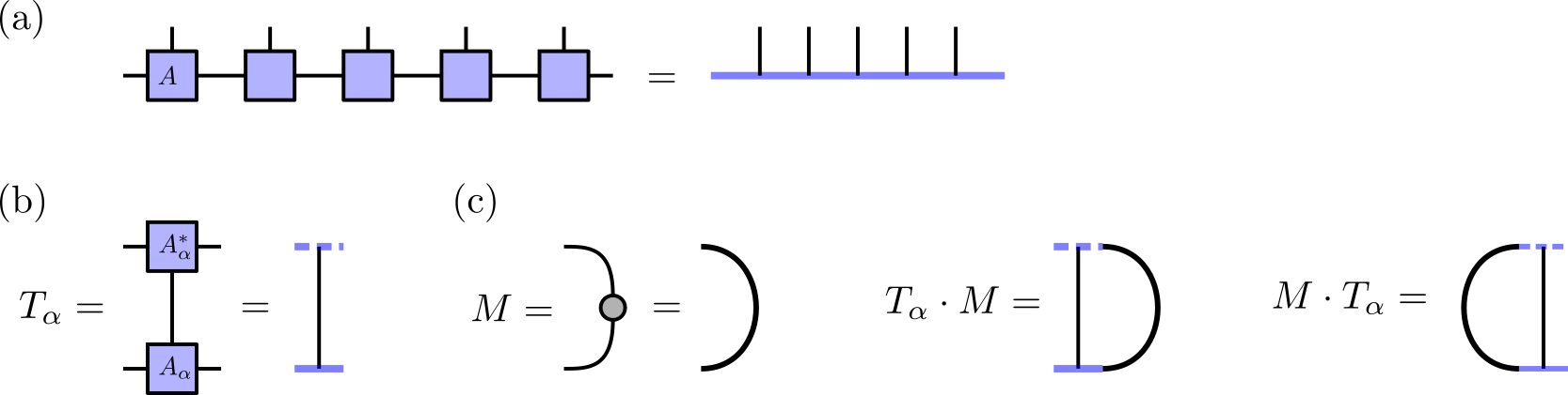
Figure 1: Matrix product states (a), transfer matrices (b), and the left and right actions of transfer matrices (c). When there is no confusion, we simplify our notation by not showing boxes representing tensors explicitly. The conjugate of the MPS matrix $A$ is represented by dotted lines.

This paper focuses on invertible states (short-range entangled states) in $(1+1)$ dimensions. In particular, we will study families of translationally-invariant invertible states that depend on a parameter $x\in X$. Such a parameterized family can be called invertible states over $X$. Invertible states in $(1+1)$ dimensions are efficiently represented as MPSs, so we begin by reviewing the necessary ingredients of MPSs. Specifically, we will deal with translationally-invariant, infinite MPSs. For a more in-depth discussion, see, for example, Refs. [22, 23, 24, 25].

As a start, let us consider a finite one-dimensional lattice with $L$ sites, labeled by $j=1,\cdots,L$. Let $\mathfrak{h}_{j}$ be a local Hilbert space with dimension $d$ (independent of $j$), where $\{\ket{i}\}_{i=1}^{d}$ is an orthonormal basis of $\mathfrak{h}_{j}$. The total Hilbert space of the chain is $\mathcal{H}:=\bigotimes_{j=1}^{L}\mathfrak{h}_{j}$. A translationally invariant MPS is defined by a set of $n\times n$ matrices $\{A^{i}\}$ with the same index as the orthonormal basis. With periodic boundary conditions, the MPS generated by $\{A^{i}\}$ is given by

$$\ket{\{A^{i}\}}_{L}:=\sum_{\{i_{k}\}}\mathrm{tr}\left(A^{i_{1}}\cdots A^{i_{L}}\right)\ket{i_{1},\ldots,i_{L}},$$ (1)

where $\sum_{\{i_{k}\}}$ represents a summation over all configurations of $(i_{1},\ldots,i_{L})$, $\sum_{\{i_{k}\}}=\sum_{i_{1}}\cdots\sum_{i_{L}}$. MPSs with fixed boundary conditions can be defined similarly with boundary vectors specifying boundary conditions.

We are interested in invertible states in the thermodynamic limit, $L\to\infty$, where boundary conditions play no role. In this limit, the physical properties of the MPS are encoded in its transfer matrix which is defined by

$$T_{A}:=\sum_{i}A^{i\ast}\otimes A^{i}.$$ (2)

A transfer matrix $T_{A}$ acts on $M\in\mathrm{Mat}_{n}(\mathbb{C})$ from the left and right as

$$T_{A}\cdot M:=\sum_{i}A^{i}MA^{i\dagger},$$ (3)

$$\quad M\cdot T_{A}:=\sum_{i}A^{i\dagger}MA^{i},$$ (4)

respectively. We represent these actions pictorially in Fig. 1.

Invertible states are represented by an injective MPS, which can be defined, using a transfer matrix, as follows [22]: Let $\{A^{i}\}$ be a set of $n\times n$ matrices and $r_{A}$ be the spectral radius of the transfer matrix. Then $\{A^{i}\}$ is injective if and only if the left action of the transfer matrix has a unique eigenvalue $\lambda$ with eigenvalue $\left|\lambda\right|=r_{A}$ and the eigenvector $\Lambda$ is a positive definite $n\times n$ matrix. We call an MPS generated by injective matrices an injective MPS. For injective matrices, it is known that the spectral radius $r^{\prime}_{A}$ for the right action is equal to $r_{A}$, i.e., $r_{A}=r^{\prime}_{A}$. In addition, a right eigenvalue $\lambda^{\prime}$ with $\left|\lambda^{\prime}\right|=r_{A}$ is unique and the corresponding eigenvector $\Lambda^{\prime}$ is a positive definite matrix.

For injective matrices, the eigenvalue equation $T_{A}\cdot\Lambda=\lambda\Lambda$ can be rewritten as

$$\sum_{i}A^{i}\Lambda A^{i\dagger}=\lambda\Lambda\quad\Longleftrightarrow\quad\sum_{i}A^{i}_{\rm c}A^{i\dagger}_{\rm c}=1_{n},$$ (5)

where $A^{i}_{\rm c}:=\frac{1}{\sqrt{\lambda}}\Lambda^{-\frac{1}{2}}A^{i}\Lambda^{\frac{1}{2}}$. We call $\{A^{i}_{\rm c}\}$ the right canonical form of the injective matrices $\{A^{i}\}$. In this form, the spectral radius for the left action (3) is $1$, and the eigenvector is modified, $\Lambda^{\prime}\to\Lambda^{-\frac{1}{2}}\Lambda^{\prime}\Lambda^{\frac{1}{2}}$, which is not the identity matrix in general.

In the following, unless otherwise mentioned, we take our MPSs to be in the right canonical form and denote the eigenvectors with eigenvalue $1$ for the left and right actions as $\Lambda^{R}_{A}$ and $\Lambda^{L}_{A}$, respectively:

$$T_{A}\cdot\Lambda^{R}_{A}=\Lambda^{R}_{A},\quad\Lambda^{L}_{A}\cdot T_{A}=\Lambda^{L}_{A}.$$ (6)

In the present case, $\Lambda^{R}_{A}$ is just the identity matrix, but in the later generalization, the case where it is not the identity matrix will appear, so we assign a symbol to it in advance.

By using the left and right eigenvectors $\Lambda_{A}^{L}$ and $\Lambda_{A}^{R}$, an infinite MPS is defined in the following manner [23, 26, 24]: For infinite systems, it is difficult to define the state itself, since an MPS on an infinite system is formally given by

$$\ket{\{A^{i}\}}_{\infty}:=\sum_{\{i_{k}\}}\cdots A^{i_{1}}\cdots A^{i_{L}}\cdots\ket{\cdots i_{1}\cdots i_{L}\cdots}$$ (7)

and its coefficients have an ambiguous infinite product of matrices. In the infinite MPS formulation, we give up defining the state itself but define the expectation value of the state. An expectation value of local observable contains infinitely many products of transfer matrices in the right and left directions (Fig. 2). Therefore, in the infinite size limit, the product only has a value on the eigenvector space of the transfer matrix with the maximum eigenvalue. So, we close the right and left ends with $\Lambda_{A}^{L}$ and $\Lambda_{A}^{R}$ to define the expectation value. For example, the inner product of $\ket{\{A^{i}\}}_{\infty}$ is defined by

$$\braket{\{A^{i}\}}{\{A^{i}\}}_{\infty}=\Lambda_{A}^{L}\cdot(T_{A})^{N}\cdot\Lambda_{A}^{R}=\mathrm{tr}\left(\Lambda_{A}^{L}\Lambda_{A}^{R}\right).$$ (8)

for arbitrary $N\in\mathbb{N}$. In the right canonical form, $\Lambda_{A}^{R}=1_{n}$ but the phase of $\Lambda_{A}^{L}$ is not fixed. As a normalization condition for the infinite MPS, we fix the phase of $\Lambda_{A}^{L}$ by $\mathrm{tr}\left(\Lambda_{A}^{L}\right)=1$. Similarly, for example, the expectation value of local operators $F_{1}$ (acting on the site $1$) and $G_{56}$ (acting on the site $5$ and $6$) are given by

$$\braket{F_{1}G_{56}}:=\Lambda_{A}^{L}\cdot T_{A}[F_{1}](T_{A})^{3}T_{A}[G_{56}]\cdot\Lambda_{A}^{R},$$ (9)

where $(T_{A}[F_{1}])_{(a,c),(b,d)}:=\sum_{i,j}A^{i\ast}_{ab}F^{ij}_{1}A^{j}_{cd}$ and $(T_{A}[G_{56}])_{(a,d),(c,f)}:=\sum_{i,j,k,l}\sum_{b,e}A^{i\ast}_{ab}A^{j\ast}_{bc}G^{ij,kl}_{56}A^{k}_{de}A^{l}_{ef}$.

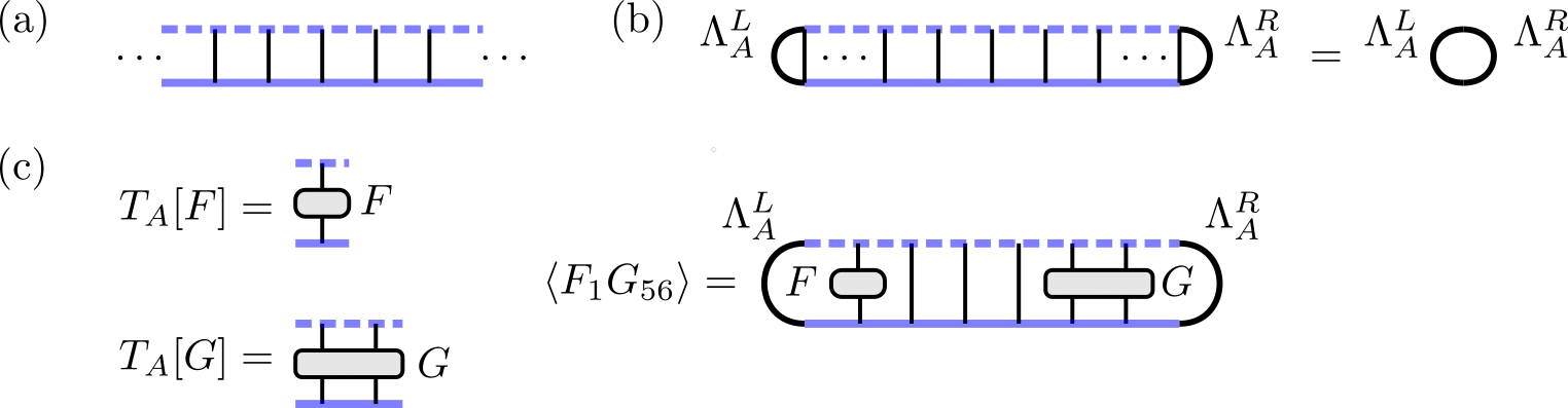
Figure 2: (a) The inner product (norm) of infinite MPSs contains infinitely many products of the transfer matrices. (b) In the thermodynamic limit, only the eigenvector with maximal eigenvalue survives. In the infinite MPS formalism, the inner product is defined by contracting the left end with the left eigenvector $\Lambda_{A}^{L}$ and the right end with the right eigenvector $\Lambda_{A}^{R}$. By using the eigenvalue equation, this value is found to be equal to $\mathrm{tr}\left(\Lambda_{A}^{L}\Lambda_{A}^{R}\right)$. (c) In general, the expectation value of a local observable is defined by putting the left eigenvector on the left side of the operator with the left-most support and the right eigenvector on the right side of the operator with the right-most support.

II.2 What Is A Gerbe and Why?

As we are interested in invertible states over $X$, we consider a family of infinite MPSs, $\{A^{i}(x)\}$, where the corresponding transfer matrix, left and right eigenvectors, etc. are also dependent on $x$. We will call such a family as MPSs over $X$.

As mentioned in Introduction, a parameterized family of quantum mechanical states with ordinary Berry phase can be described by a complex line bundle. Let us consider an open covering of $X$, $\{U_{\alpha}\}$. A complex line bundle is defined by transition functions $e^{i2\pi\phi_{\alpha\beta}}$ on intersections $U_{\alpha\beta}:=U_{\alpha}\cap U_{\beta}$. They satisfy $e^{i2\pi\phi_{\beta\alpha}}=e^{-i2\pi\phi_{\alpha\beta}}$, and also, on triple intersections $U_{\alpha\beta\gamma}:=U_{\alpha}\cap U_{\beta}\cap U_{\gamma}$,

$$e^{i2\pi\phi_{\alpha\beta}}e^{i2\pi\phi_{\beta\gamma}}e^{i2\pi\phi_{\gamma\alpha}}=1.$$ (10)

A transition function $e^{i2\pi\phi_{\alpha\beta}}$ is an element of the Čeck complex $C^{1}(X;\underline{\mathrm{U}(1)})$ and Eq. (10) is nothing but the cocycle condition. Therefore, $e^{i2\pi\phi_{\alpha\beta}}$ defines a $1$st Čeck cohomology class $\left[e^{i2\pi\phi_{\alpha\beta}}\right]\in\mathrm{H}^{1}(X;\underline{\mathrm{U}(1)})\simeq\mathrm{H}^{2}(X;\mathbb{Z})$, and it is measured by the $1$st Chern class. Here, the underbar represents that it is the sheaf cohomology.

In this paper, we consider a higher generalization of the Berry phase for a parameterized family of $(1+1)$-dimensional invertible states [12, 27, 19]. We expect that these higher generalizations of the Thouless pumping can be topologically classified by the Dixmier-Douady class that takes its value in $\mathrm{H}^{3}(X;\mathbb{Z})$. We propose that the mathematical structure that describes the topological classification of higher Thouless pumping is a gerbe. A gerbe is a higher generalization of a complex line bundle. It has been used to describe, for example, the $(1+1)$-dimensional Wess-Zumino-Witten models, the $(2+1)$-dimensional Chern-Simons theories, the Kalb-Ramond $B$-field and D-branes in string theory, and various anomalies in quantum field theory [28, 29, 30]. Let us first briefly introduce the mathematical definition of a gerbe. In the next subsection, we will then construct a gerbe from MPSs over $X$.

Let $X$ be a topological space. A gerbe on $X$ is described by datum $(\{U_{\alpha}\},\{L_{\alpha\beta}\},\{\sigma_{\alpha\beta\gamma}\})$ that satisfies following conditions [31]: $\{U_{\alpha}\}$ is an open covering of a base space $X$, $L_{\alpha\beta}$ is a complex vector bundle over $U_{\alpha\beta}$, and $\sigma_{\alpha\beta\gamma}:L_{\alpha\beta}\otimes L_{\beta\gamma}\to L_{\alpha\gamma}$ is an isomorphism between complex vector bundles. They satisfy a commutative diagram

$$\begin{CD}L_{\alpha\beta}\otimes L_{\beta\gamma}\otimes L_{\gamma\delta}@>{1\otimes\sigma_{\beta\gamma\delta}}>{}>L_{\alpha\beta}\otimes L_{\beta\delta}\\ @V{\sigma_{\alpha\beta\gamma}}V{}V@V{\sigma_{\alpha\beta\delta}}V{}V\\ L_{\alpha\gamma}\otimes L_{\gamma\delta}@>{\sigma_{\alpha\gamma\delta}}>{}>L_{\alpha\delta}.\end{CD}$$ (11)

It is known that gerbes on a topological space $X$ are classified by $\mathrm{H}^{3}(X;\mathbb{Z})$ [32]. This is a primary reason that we expect a gerbe is an underlying mathematical structure for parameterized $(1+1)$-dimensional invertible states and MPSs over $X$, and, by constructing a gerbe from a family of $(1+1)$-dimensional systems, we can extract a topological invariant that takes its value in $\mathrm{H}^{3}(X;\mathbb{Z})$.

II.3 Definition of A Constant Rank MPS Gerbe

Let’s construct a gerbe on $X$ from a family of injective MPS matrices parametrized by $X$. For simplicity, we will first keep the rank (bond dimension) of MPSs constant. We will drop this condition later in Sec. II.5.

To set the stage, we fix an open covering $\{U_{\alpha}\}_{\alpha\in I}$ of $X$ and consider $n\times n$ injective MPS matrices $\{A^{i}_{\alpha}(x)\}$ on each $U_{\alpha}$. At the intersection of two patches, $U_{\alpha\beta}$, we have two MPSs representing the same physical state defined at $x\in X$. By the fundamental theorem for (bosonic) MPSs, these two MPSs are related by a gauge transformation,

$$A^{i}_{\alpha}(x)=g_{\alpha\beta}(x)A^{i}_{\beta}(x)g_{\alpha\beta}^{\dagger}(x),$$ (12)

where $g_{\alpha\beta}$ is an element of the projective unitary group, $g_{\alpha\beta}\in\mathrm{PU}(n)$. We call $g_{\alpha\beta}$ a transition function. Let’s take a $\mathrm{U}(n)$-lift $\{\hat{g}_{\alpha\beta}\}$ of $\{g_{\alpha\beta}\}$. From this unitary matrices $\{\hat{g}_{\alpha\beta}\}$, we define a state over $U_{\alpha\beta}$ by

$$\ket{\{\hat{g}_{\alpha\beta}\}}:=\sum_{\{i_{k}\}}\cdots A^{i_{1}}_{\alpha}\cdots A^{i_{p}}_{\alpha}\hat{g}_{\alpha\beta}A^{i_{p+1}}_{\beta}\cdots A^{i_{L}}_{\beta}\cdots\ket{\cdots i_{1}\cdots i_{i_{L}}\cdots}.$$ (13)

Here, because of a translation symmetry, the right-hand side does not depend on $p\in\mathbb{Z}$. Although this vector contains ambiguous infinite products in its coefficients, when calculating physical quantities (such as the higher Berry phase), as we will see below, we extract them by contracting the ends using suitable eigenvectors of suitable transfer matrices. The state $\ket{\{\hat{g}_{\alpha\beta}\}}$ is reminiscent of the so-called mixed gauge MPS. We also define a complex line bundle over $U_{\alpha\beta}$ by

$$L_{\hat{g}_{\alpha\beta}}:=\mathbb{C}\ket{\{\hat{g}_{\alpha\beta}\}}.$$ (14)

Finally, on a triple intersection $U_{\alpha\beta\gamma}$, we define an isomorphism

$$\sigma_{\alpha\beta\gamma}^{\rm MPS}:L_{\hat{g}_{\alpha\beta}}\otimes L_{\hat{g}_{\beta\gamma}}\to L_{\hat{g}_{\alpha\gamma}}:\ket{\{\hat{g}_{\alpha\beta}\}}\otimes\ket{\{\hat{g}_{\beta\gamma}\}}\mapsto\ket{\{\hat{g}_{\alpha\beta}\hat{g}_{\beta\gamma}\}}.$$ (15)

Let’s check the commutative diagram Eq. (11) for $(\{U_{\alpha}\},\{L_{\hat{g}_{\alpha\beta}}\},\{\sigma_{\alpha\beta\gamma}^{\rm MPS}\})$: There exists $c_{\alpha\beta\gamma}\in\mathrm{U}(1)$ on $U_{\alpha\beta\gamma}$ so that

$$\hat{g}_{\alpha\beta}\hat{g}_{\beta\gamma}=c_{\alpha\beta\gamma}\hat{g}_{\alpha\gamma}.$$ (16)

Since $\ket{\{\hat{g}_{\alpha\beta}\hat{g}_{\beta\gamma}\}}=c_{\alpha\beta\gamma}\ket{\{\hat{g}_{\alpha\gamma}\}}$, Eq. (11) is equivalent to $(\delta c)_{\alpha\beta\gamma\delta}:=c_{\alpha\beta\gamma}c_{\alpha\beta\delta}^{\ast}c_{\alpha\gamma\delta}c_{\beta\gamma\delta}^{\ast}=1$, and this equation follows from the associativity of the matrix product. Therefore, $(\{U_{\alpha}\},\{L_{\hat{g}_{\alpha\beta}}\},\{\sigma_{\alpha\beta\gamma}^{\rm MPS}\})$ is a gerbe on $X$. Since $(\delta c)_{\alpha\beta\gamma\delta}=1$, $c_{\alpha\beta\gamma}$ defines a $2$nd Čeck cohomology class $\left[c_{\alpha\beta\gamma}\right]\in\mathrm{H}^{2}(X;\underline{\mathrm{U}(1)})\simeq\mathrm{H}^{3}(X;\mathbb{Z})$. $\left[c_{\alpha\beta\gamma}\right]$, which is a topological invariant of a gerbe, and called the Dixmier-Douady class [33]. In the following, we call $(\{U_{\alpha}\},\{L_{\hat{g}_{\alpha\beta}}\},\{\sigma_{\alpha\beta\gamma}^{\rm MPS}\})$ a constant-rank MPS gerbe. Here, the adjective constant-rank implies the bond dimension of MPS matrices is constant over the parameter space $X$.

A constant-rank MPS gerbe is a proper mathematical structure to describe invertible states over $X$ when we are interested in a torsion part of $\mathrm{H}^{3}(X;\mathbb{Z})$, i.e., a finite order subgroup of $\mathrm{H}^{3}(X;\mathbb{Z})$. Such cases have been studied in detail in Ref. [19]. In general, however, the rank of MPS matrices may not be constant over the parameter space $X$ [34]. Moreover, constant-rank MPS matrices cannot describe nontrivial models which take their values in the free part, i.e., (copies of) the infinite cyclic group $\mathbb{Z}$, of $\mathrm{H}^{3}(X;\mathbb{Z})$. Let us briefly explain this point. Since $\hat{g}_{\alpha\beta}\hat{g}_{\beta\gamma}=c_{\alpha\beta\gamma}\hat{g}_{\alpha\gamma}$ holds as a unitary matrix, the following equation is obtained by taking the determinant of both sides:

$$\det(\hat{g}_{\alpha\beta})\det(\hat{g}_{\alpha\gamma})^{\ast}\det(\hat{g}_{\beta\gamma})=c_{\alpha\beta\gamma}^{n}.$$ (17)

This equation implies that $c_{\alpha\beta\gamma}^{n}$ is closed cocycle and $[c_{\alpha\beta\gamma}^{n}]$ is trivial in $\mathrm{H}^{2}(X;\underline{\mathrm{U}(1)})$, i.e., $[c_{\alpha\beta\gamma}^{n}]=1\in\mathrm{H}^{2}(X;\underline{\mathrm{U}(1)})$. Therefore, the topological class of $(\{U_{\alpha}\},\{L_{\hat{g}_{\alpha\beta}}\},\{\sigma_{\alpha\beta\gamma}^{\rm MPS}\})$ is in the torsion part of $\mathrm{H}^{3}(X;\mathbb{Z})$. This is due to the mathematical fact that the topological class of a $\mathrm{PU}(n)$-bundle can only take its value in the torsion part of $\mathrm{H}^{3}(X;\mathbb{Z})$ [35]. Therefore, we need to handle a family of MPS matrices with a non-constant rank and construct a gerbe from such matrices. We discuss this point in Sec. II.4.

II.4 Triple Inner Product of MPSs

Before delving into non-constant-rank MPSs, let us discuss one more ingredient, still using constant-rank MPSs. Specifically, we will demonstrate how the data that makes up the MPS gerbe, such as the transition functions and the Dixmier-Douady class, relate to certain overlaps of MPSs. We will show that the Dixmier-Douady class can be obtained from the triple inner product, defined below, for three MPSs. This is reminiscent of Wu-Yang’s work on U(1) magnetic monopoles, where a topological invariant, the Chern class, can be obtained from the inner product of two wave functions from different patches. In this discussion, we present an alternative formulation in which the MPS gerbe’s data is expressed in terms of (triple) wave function overlaps. Moreover, in the following section, we’ll see that this formulation also naturally generalizes to a definition of a gerbe from MPSs over $X$ with a non-constant rank.

Let us start with the transfer matrix at $x\in U_{\alpha}$ is defined by

$$T_{\alpha}(x)=\sum_{i}A^{i\ast}_{\alpha}(x)\otimes A^{i}_{\alpha}(x).$$ (19)

As reviewed in Sec. II.1, $T_{\alpha}(x)$ acts on $\mathrm{Mat}_{n}(\mathbb{C})$ from the left and right as $T_{\alpha}(x)\cdot M:=\sum_{i}A^{i}_{\alpha}(x)MA^{i\dagger}_{\alpha}(x)$, $M\cdot T_{\alpha}(x):=\sum_{i}A^{i\dagger}_{\alpha}(x)MA^{i}_{\alpha}(x)$, respectively, for arbitrary $M\in\mathrm{Mat}_{n}(\mathbb{C})$. We represent this action pictorially as in Fig. 1. The transfer matrix $T_{\alpha}(x)$ has unique right and left eigenvectors $\Lambda^{R}_{\alpha}(x)$ and $\Lambda^{L}_{\alpha}(x)$ with eigenvalue $1$:

$$T_{\alpha}(x)\cdot\Lambda^{R}_{\alpha}(x)=\Lambda^{R}_{\alpha}(x),\quad\Lambda^{L}_{\alpha}(x)\cdot T_{\alpha}(x)=\Lambda^{L}_{\alpha}(x).$$ (20)

A primary tool in this section is a mixed transfer matrix, which we define from $\{A^{i}_{\alpha}(x)\}$ and $\{A^{i}_{\beta}(x)\}$ as

$$T_{\alpha\beta}(x):=\sum_{i}A^{i\ast}_{\beta}(x)\otimes A^{i}_{\alpha}(x),$$ (21)

over $U_{\alpha\beta}$. A crucial point is that the spectrum of $T_{\alpha\beta}(x)$ is identical to that of $T_{\alpha}(x)$, and in particular, $T_{\alpha\beta}(x)$ has unique left and right eigenvectors with eigenvalue $1$. Let’s check this point. From now on, we omit the dependence on $x$. Let $\Lambda_{\alpha}^{R,k}$ be the $k$-th eigenvector of $T_{\alpha}$ with eigenvalue $\lambda_{\alpha}^{R,k}$, $T_{\alpha}\cdot\Lambda_{\alpha}^{R,k}=\lambda_{\alpha}^{R,k}\Lambda_{\alpha}^{R,k}.$ Then $\Lambda_{\alpha\beta}^{R,k}:=\Lambda_{\alpha}^{R,k}\hat{g}_{\alpha\beta}$ is the eigenvector of $T_{\alpha\beta}$ with the same eigenvalue $\lambda_{\alpha}^{R,k}$:

$$T_{\alpha\beta}\cdot\Lambda_{\alpha\beta}^{R,k}=\sum_{i}A^{i}_{\alpha}(\Lambda_{\alpha}^{R,k}\hat{g}_{\alpha\beta})(\hat{g}_{\beta\alpha}A^{i\dagger}_{\alpha}\hat{g}_{\beta\alpha}^{\dagger})=\lambda_{\alpha}^{R,k}\Lambda_{\alpha}^{R,k}\hat{g}_{\beta\alpha}^{\dagger}=\lambda_{\alpha}^{R,k}\Lambda_{\alpha\beta}^{R,k}.$$ (22)

Therefore, there is a one-to-one correspondence between the eigenvectors of $T_{\alpha}$ and $T_{\alpha\beta}$ with the same eigenvalue. Similarly, for a left eigenvector $\Lambda_{\alpha}^{L,k}$ of $T_{\alpha}$ with eigenvalue $\lambda_{\alpha}^{L,k}$, $\Lambda_{\alpha\beta}^{L,k}:=\hat{g}_{\beta\alpha}\Lambda_{\alpha}^{L,k}$ is a left eigenvector of $T_{\alpha\beta}$ with the eigenvalue $\lambda_{\alpha}^{L,k}$:

$$\Lambda_{\alpha\beta}^{L,k}\cdot T_{\alpha\beta} =\sum_{i}(\hat{g}_{\beta\alpha}A^{i\dagger}_{\alpha}\hat{g}_{\beta\alpha}^{\dagger})\hat{g}_{\beta\alpha}\Lambda_{\alpha}^{L,k}A^{i}_{\alpha}=\lambda_{\alpha}^{L,k}\hat{g}_{\beta\alpha}\Lambda_{\alpha}^{L,k}=\lambda_{\alpha}^{L,k}\Lambda_{\alpha\beta}^{L,k}.$$ (23)

We define the right and left eigenstates of $T_{\alpha\beta}$ with eigenvalue $1$ by

$$\Lambda_{\alpha\beta}^{R}:=\Lambda_{\alpha}^{R}\hat{g}_{\alpha\beta}=\hat{g}_{\alpha\beta}\Lambda_{\beta}^{R},\quad\Lambda_{\alpha\beta}^{L}:=\hat{g}_{\beta\alpha}\Lambda_{\alpha}^{L}=\Lambda_{\beta}^{L}\hat{g}_{\beta\alpha}.$$ (24)

We represent the eigenvalue equations pictorially as in Fig. 3.

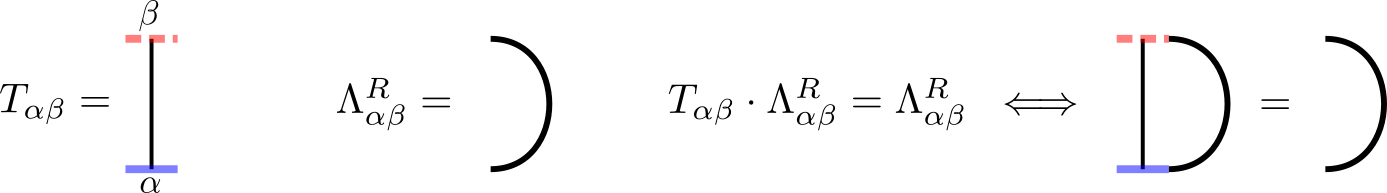
Figure 3: The mixed transfer matrix $T_{\alpha\beta}$ and its right eigenvalue equation.

In the right canonical form, $\Lambda^{R}_{\alpha}=1_{n}$. We also fix the phase of $\Lambda^{L}_{\alpha}$ by the condition $\mathrm{tr}\left(\Lambda^{L}_{\alpha}\right)=1$. This is the normalization condition of the infinite MPS. Remark that the phases of $\Lambda_{\alpha\beta}^{R}$ and $\Lambda_{\alpha\beta}^{L}$ are still redundant, but the redefinition of them can be absorbed in the $\mathrm{U}(n)$-lift of the transition functions.

We are now ready to define the triple inner product. On a triple intersection $U_{\alpha\beta\gamma}$, consider the ”boomerang” diagram as in Fig. 4. Here, three infinite MPSs, representing the same physical state at $x\in X$, from three different patches are ”glued” together as in Fig. 4. Observe how ”bra” and ”ket” MPS matrices are arranged depending on which ”wing” they are located. At the infinities of the three ”wings”, the tensor network is capped off by putting either left or right eigenvectors. The products of the mixed transfer matrices are easily computed in the thermodynamic limit, and we can check that the boomerang diagram computes the Dixmier-Douady class:

$$\text{the boomerang diagram}=\mathrm{tr}\left(\Lambda_{\beta\alpha}^{L}\Lambda_{\beta\gamma}^{R}\Lambda_{\gamma\alpha}^{R}\right)=\mathrm{tr}\left(\Lambda_{\alpha}^{L}\hat{g}_{\alpha\beta}1_{n}\hat{g}_{\beta\gamma}1_{n}\hat{g}_{\gamma\alpha}\right)=c_{\alpha\beta\gamma}.$$ (25)

We define the triple inner product of three MPSs as the ”boomerang” diagram and the higher Berry phase as the Dixmier Douady class. The ordinary Berry phase can be obtained from the ordinary inner product of two wavefunctions that are physically the same but taken from two different patches. As the natural generalization of this method, the higher Berry phase in $(1+1)$-dimensional systems can be obtained from the triple inner product of three MPSs that are physically the same but taken from three different patches. Note that with the mixed transfer matrix and the triple inner product, it is not necessary to deal with the transition functions explicitly. Instead, the data necessary to define the (constant-rank) MPS gerbe are encoded in the mixed transfer matrix and the triple inner product.

Finally, we note that there are some ambiguities in the definition of an MPS gerbe and a triple inner product. For example, a gerbe can be constructed by using $\Lambda^{L}_{\beta\alpha}$ instead of $\Lambda^{R}_{\alpha\beta}$ in the definition of the line bundle on $U_{\alpha\beta}$. In our choice, $|\{A^{i}_{\alpha}\}\rangle$, $|\{\hat{g}_{\alpha\beta}\}\rangle$ and the modulus of the triple inner product are all normalized to be one, while in other choices we would need to adjust normalization (by properly rescaling $\Lambda^{L}_{\beta\alpha}$). Our choice would be natural in this sense.

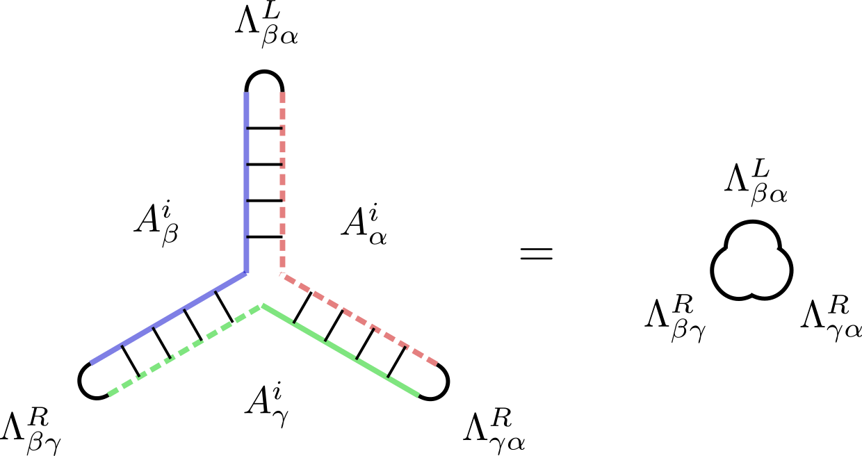
Figure 4: The triple inner product of three MPSs $\{A^{i}_{\alpha}\}$, $\{A^{i}_{\beta}\}$, $\{A^{i}_{\gamma}\}$ from different patches $U_{\alpha},U_{\beta},U_{\gamma}$, respectively. The right side of the middle wing and the right side of the bottom right wing represent the matrix $A^{i}_{\alpha}$, the left side of the middle wing and the left side of the bottom left wing represent the matrix $A^{i}_{\beta}$, and the right side of the bottom left wing and the left side of the bottom right wing represent the matrix $A^{i}_{\gamma}$. The dotted lines represent the complex conjugation of the MPS matrices.

II.5 Definition of A Non-Constant Rank MPS Gerbe

In Secs.  II.3 and II.4, we assume that the rank of the MPS matrices is constant over the parameter space $X$. As a generalization of this situation, we consider a family of MPS matrices with non-constant rank. To this end, we first introduce a notion of essentially injective matrices: let $\{A^{i}\}$ be a set of $n\times n$ matrices. Then $\{A^{i}\}$ is essentially injective if and only if there is an invertible matrix $X$ such that

$$XA^{i}X^{-1}=\begin{pmatrix}\tilde{A}^{i}&0\\ Y^{i}&0\end{pmatrix},$$ (26)

for some $\tilde{n}\times\tilde{n}$ injective matrices $\{\tilde{A}^{i}\}$ and $(n-\tilde{n})\times\tilde{n}$ matrices $Y^{i}$. Also, we impose the right canonical form condition, $\sum_{i}A^{i}A^{i\dagger}=1_{n}$. In terms of $\{\tilde{A}^{i}\}$ and $Y_{i}$, this means that

$$\sum_{i}\tilde{A}^{i}\tilde{A}^{i\dagger}=1_{\tilde{n}},\quad\sum Y^{i}Y^{i\dagger}=1_{n-\tilde{n}},$$

$$\sum_{i}Y^{i}\tilde{A}^{i\dagger}=0,\quad\sum_{i}\tilde{A}^{i}Y^{i\dagger}=0.$$ (27)

We call $\tilde{n}$ an essential rank of the essentially injective matrices, and $\{\tilde{A}^{i}\}$ the injective part of the essentially injective matrices. Usually, we eliminate the lower triangular component $Y^{i}$ by hand because it does not affect the state. However, such cases appear naturally when considering a family of MPS matrices.

Let $\{U_{\alpha}\}$ be an open covering of $X$ and let’s consider a family of essentially injective MPS matrices. Assume that the rank of MPS matrices is constant on each patch. Let $\{A^{i}_{\alpha}\}$ be $n_{\alpha}\times n_{\alpha}$ essentially injective matrices whose essential rank $\tilde{n}_{\alpha}(x)$ can be dependent on $x\in U_{\alpha}$. We also assume that $\tilde{n}_{\alpha}(x)=\tilde{n}_{\beta}(x)$ on non-empty intersection $U_{\alpha\beta}$. Let’s consider the mixed transfer matrix

$$T_{\alpha\beta}=\sum_{i}A^{i\ast}_{\beta}\otimes A^{i}_{\alpha}.$$ (28)

The mixed transfer matrix $T_{\alpha\beta}$ acts on $M\in\mathrm{Mat}_{n_{\alpha}\times n_{\beta}}(\mathbb{C})$ from the left as

$$T_{\alpha\beta}\cdot M=\sum_{i}A^{i}_{\alpha}MA^{i\dagger}_{\beta},$$ (29)

and acts on $M\in\mathrm{Mat}_{n_{\beta}\times n_{\alpha}}(\mathbb{C})$ from the right as

$$M\cdot T_{\alpha\beta}=\sum_{i}A^{i\dagger}_{\beta}MA^{i}_{\alpha}.$$ (30)

Then we can show that both the maximal left and right eigenvalues of the mixed transfer matrix are $1$, and the right and left eigenvectors $\Lambda_{\alpha\beta}^{R}$ and $\Lambda_{\alpha\beta}^{L}$ are unique and given by

$$\Lambda_{\alpha\beta}^{R}:=\begin{pmatrix}\tilde{\Lambda}_{\alpha\beta}^{R}&0\\ 0&\sum_{i}Y^{i}_{\alpha}\tilde{\Lambda}^{R}_{\alpha\beta}Y^{i\dagger}_{\beta}\end{pmatrix}\quad\mbox{and}\quad\Lambda_{\alpha\beta}^{L}:=\begin{pmatrix}\tilde{\Lambda}_{\alpha\beta}^{L}&0\\ 0&0\end{pmatrix},$$ (31)

respectively, where $\tilde{\Lambda}_{\alpha\beta}^{R}$ and $\tilde{\Lambda}_{\alpha\beta}^{L}$ are right and left eigenvectors with eigenvalue $1$ of the mixed transfer matrix of injective part of $\{A^{i}_{\alpha}\}$ and $\{A^{i}_{\beta}\}$.

This can be readily checked as follows. Let $M$ be an $n_{\alpha}\times n_{\beta}$ matrix and consider the following decomposition:

$$M=\begin{pmatrix}\Lambda&Z\\ X&\Lambda^{\prime}\end{pmatrix},$$ (32)

where $\Lambda$, $X$, $Z$, and $\Lambda^{\prime}$ are $\tilde{n}_{\alpha}\times\tilde{n}_{\alpha}$, $(n_{\alpha}-\tilde{n}_{\alpha})\times\tilde{n}_{\alpha}$, $\tilde{n}_{\alpha}\times(n_{\beta}-\tilde{n}_{\alpha})$, and $(n_{\alpha}-\tilde{n}_{\alpha})\times(n_{\beta}-\tilde{n}_{\alpha})$, respecitvely. Then, the right eigenvalue equation $T_{\alpha\beta}\cdot M=M$ reads

$$\sum_{i}\begin{pmatrix}\tilde{A}^{i}_{\alpha}\Lambda\tilde{A}^{i\dagger}_{\beta}&\tilde{A}^{i}_{\alpha}\Lambda Y^{i\dagger}_{\beta}\\ Y^{i}_{\alpha}\Lambda\tilde{A}^{i\dagger}_{\beta}&Y^{i}_{\alpha}\Lambda Y^{i\dagger}_{\beta}\end{pmatrix}=\begin{pmatrix}\Lambda&Z\\ X&\Lambda^{\prime}\end{pmatrix}.$$ (33)

From the upper left block, we see that $\Lambda$ must be the right eigenvector, $\Lambda=\Lambda^{R}_{\alpha\beta}=g_{\alpha\beta}$. We also see from the lower left block $\sum_{i}Y^{i}_{\alpha}\Lambda\tilde{A}^{i\dagger}_{\beta}=\sum_{i}Y^{i}_{\alpha}g_{\alpha\beta}\tilde{A}^{i\dagger}_{\beta}=\sum_{i}Y^{i}_{\alpha}\tilde{A}^{i\dagger}_{\alpha}g^{\dagger}_{\alpha\beta}=0$ where we used the right canonical condition (II.5). We can show similarly that $\sum_{i}\tilde{A}^{i}_{\alpha}\Lambda Y^{i\dagger}_{\beta}=g_{\alpha\beta}\sum_{i}\tilde{A}^{i}_{\beta}Y^{i\dagger}_{\beta}=0$. We thus conclude the first equation in (31). For the left eigenequation $M\cdot T_{\alpha\beta}=M$, we consider the similar decomposition (32), which leads to

$$\sum_{i}\begin{pmatrix}(\tilde{A}^{i\dagger}_{\beta}\Lambda+Y^{i\dagger}_{\beta}X)\tilde{A}^{i}_{\alpha}+(\tilde{A}^{i\dagger}_{\beta}Z+Y^{i\dagger}_{\beta}\Lambda^{\prime})Y^{i}_{\alpha}&0\\ 0&0\end{pmatrix}=\begin{pmatrix}\Lambda&Z\\ X&\Lambda^{\prime}\end{pmatrix}.$$ (34)

The solution is given by the second equation in (31), $X=Z=\Lambda^{\prime}=0$ and $\Lambda=\tilde{\Lambda}^{L}_{\alpha\beta}$.

We are now ready to define a gerbe from a family of essentially injective matrices, including the case where the rank is not constant over the parameter space. It is defined, as a natural generalization of a constant-rank MPS gerbe, as follows: We define a state over $U_{\alpha\beta}$ by

$$\ket{\{\Lambda^{R}_{\alpha\beta}\}}:=\sum_{\{i_{k}\}}\cdots A^{i_{1}}_{\alpha}\cdots A^{i_{p}}_{\alpha}\Lambda^{R}_{\alpha\beta}A^{i_{p+1}}_{\beta}\cdots A^{i_{L}}_{\beta}\cdots\ket{\cdots i_{1}\cdots i_{i_{L}}\cdots},$$ (35)

and a complex line bundle over $U_{\alpha\beta}$ by

$$L^{\rm MPS}_{\alpha\beta}:=\mathbb{C}\ket{\{\Lambda^{R}_{\alpha\beta}\}}.$$ (36)

On a triple intersection, we define an isomorphism

$$\sigma_{\alpha\beta\gamma}^{\rm MPS}:L^{\rm MPS}_{\alpha\beta}\otimes L^{\rm MPS}_{\beta\gamma}\to L^{\rm MPS}_{\alpha\gamma}:\ket{\{\Lambda^{R}_{\alpha\beta}\}}\otimes\ket{\{\Lambda^{R}_{\beta\gamma}\}}\mapsto\ket{\{\Lambda^{R}_{\alpha\beta}\Lambda^{R}_{\beta\gamma}\}}=c_{\alpha\beta\gamma}\ket{\{\Lambda^{R}_{\alpha\gamma}\}}.$$ (37)

Then, $\mathcal{G}^{\rm MPS}:=(\{U_{\alpha}\},\{L^{\rm MPS}_{\alpha\beta}\},\{\sigma^{\rm MPS}_{\alpha\beta\gamma}\})$ is a gerbe on $X$. We call $\mathcal{G}^{\rm MPS}$ a non-constant-rank MPS gerbe or an MPS gerbe for short. The triple inner product can also be defined following the constant-rank case. We can compute the Dixmier-Douady class by the same diagram as in the Fig. 4:

$$\text{the boomerang diagram}=\mathrm{tr}\left(\Lambda_{\beta\alpha}^{L}\Lambda_{\beta\gamma}^{R}\Lambda_{\gamma\alpha}^{R}\right)=c_{\alpha\beta\gamma}.$$ (38)

Since $\{\Lambda^{L}_{\alpha\beta}\}$ includes the projection onto the injective part and $\{\Lambda^{R}_{\alpha\beta}\}$ is block-diagonal, Eq. (38) reduces to

$$\mathrm{tr}\left(\Lambda_{\beta\alpha}^{L}\Lambda_{\beta\gamma}^{R}\Lambda_{\gamma\alpha}^{R}\right)=\mathrm{tr}\left(\tilde{\Lambda}_{\beta\alpha}^{L}\tilde{\Lambda}_{\beta\gamma}^{R}\tilde{\Lambda}_{\gamma\alpha}^{R}\right).$$ (39)

Namely, $c_{\alpha\beta\gamma}$ is nothing but the Dixmier-Douady class for the MPS matrices projected onto the injective part.

III Star Product and Integration

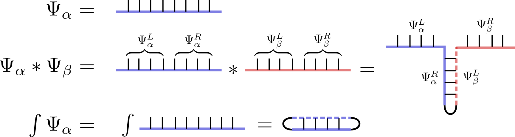
Figure 5: Matrix product states, $*$ product and integration. Along the dotted lines, the relevant MPS tensors are conjugated, i.e., $A^{*}$.

In this section, we introduce two operations for infinite MPSs – star product ($*$) and integration ($\int$). As we will see, these operators are useful for describing the structures introduced in the preceding sections. Our definitions are largely inspired by, and essentially identical to, the non-commutative geometry in string field theory [37].

Let us first introduce a multiplication law $*$ for two infinite MPSs (Fig. 5). In this section, we denote an MPS constructed from $\{A^{i}_{\alpha}\}$ as $\Psi_{{\alpha}}$. For two MPSs $\Psi_{{\alpha}}$ and $\Psi_{{\beta}}$ from different patches $U_{\alpha}$ and $U_{\beta}$, the product $\Psi_{{\alpha}}*\Psi_{{\beta}}$ is defined by first splitting $\Psi_{{\alpha}}$ and $\Psi_{{\beta}}$ into their left and right pieces, denoted by $\Psi^{L}_{\alpha},\Psi^{R}_{\alpha}$ and $\Psi^{L}_{\beta}$ and $\Psi^{R}_{\beta}$, respectively. In the product $\Psi_{{\alpha}}*\Psi_{{\beta}}$, $\Psi^{R}_{\alpha}$ and $\Psi^{L}_{\beta}$ are ”glued”, i.e., contracted. In this process, the MPS matrices $\{A^{i}_{\beta}\}$ on the left part of $\Psi_{\beta}$ are first converted to their conjugates $\{A^{i*}_{\beta}\}$ (”bras”) and then contracted with the right part of $\Psi_{\alpha}$. The star product is associative, $(\Psi_{{\alpha}}*\Psi_{{\beta}})*\Psi_{{\gamma}}=\Psi_{{\alpha}}*(\Psi_{{\beta}}*\Psi_{{\gamma}})$, but not commutative. Intuitively, we regard physical indices in $\Psi^{L}_{\alpha}$ and $\Psi^{R}_{\alpha}$ as row (input) and column (output) indices of an infinite matrix, or a semi-infinite matrix product operator. Accordingly, the $*$ product can be interpreted as matrix multiplication of two infinite-dimensional matrices.

To see the connection with the MPS gerbe, we consider three MPSs $\Psi_{{\alpha}},\Psi_{{\beta}},\Psi_{{\gamma}}$ defined on patches $U_{\alpha},U_{\beta},U_{\gamma}$, respectively. First, we can readily check that the product $\Psi_{{\alpha}}*\Psi_{{\beta}}$ is nothing but the mixed gauge MPS, $|\{\Lambda^{R}_{\alpha\beta}\}\rangle$. Following the notation of this section, we simply write $|\{\Lambda^{R}_{\alpha\beta}\}\rangle\equiv\Psi_{{\alpha\beta}}$. We also note that an infinite canonical MPS is an idempotent of the $*$ product, $\Psi_{{\alpha}}*\Psi_{{\alpha}}=\Psi_{{\alpha}}$. Second, the product of $\Psi_{{\alpha\beta}}$ and $\Psi_{{\beta\gamma}}$ is given by

$$\Psi_{{\alpha\beta}}*\Psi_{{\beta\gamma}}=\Psi_{{\alpha}}*\Psi_{{\beta}}*\Psi_{{\beta}}*\Psi_{{\gamma}}=c_{\alpha\beta\gamma}\Psi_{{\alpha\gamma}}.$$ (40)

Hence, the $*$ product is nothing but $\sigma^{{\rm MPS}}_{\alpha\beta\gamma}$. We note that mixed gauge MPSs are closed under the multiplication $*$.

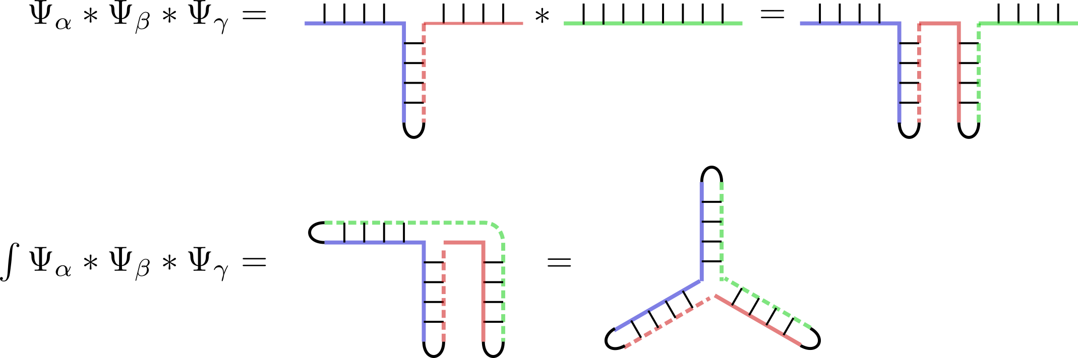
Figure 6: The star product of three MPSs $\Psi_{\alpha}$, $\Psi_{\beta}$, and $\Psi_{\gamma}$, and the triple inner product.

To see how the triple inner product arises, we also introduce an ”integration” $\int$. To define the integration of $\Psi_{\alpha}$, $\int\Psi_{\alpha}$, we ”fold” $\Psi_{{\alpha}}$ and contract $\Psi^{L}_{\alpha}$ and $\Psi^{R}_{\alpha}$ (Fig. 5). With this rule, we can see, for example,

$$\int\,\displaystyle\Psi_{{\alpha}} =\mathrm{tr}\,(\Lambda^{L}_{\alpha}\Lambda^{R}_{\alpha})=1,$$

$$\int\Psi_{{\alpha}}*\Psi_{{\beta}} =\mathrm{tr}\,(\Lambda^{L}_{\alpha\beta}\Lambda^{R}_{\alpha\beta})=\mathrm{tr}\,(\Lambda^{L}_{\beta}\hat{g}_{\beta\alpha}\hat{g}_{\alpha\beta}\Lambda^{R}_{\beta})=1.$$ (41)

Namely, $\int\Psi_{{\alpha}}$ is the norm of $\Psi_{{\alpha}}$ and $\int\Psi_{{\alpha}}*\Psi_{{\beta}}$ is the overlap of $\Psi_{{\alpha}}$ and $\Psi_{{\beta}}$. It is also evident that $\int\Psi_{{\alpha}}*\Psi_{{\beta}}=\int\Psi_{{\beta}}*\Psi_{{\alpha}}$. As before, regarding the physical indices in $\Psi^{L}_{\alpha}$ and $\Psi^{R}_{\alpha}$ as row and column indices, the integration is interpreted as the matrix trace. Finally, we can readily see that the integral of the triple product $\Psi_{{\alpha}}*\Psi_{{\beta}}*\Psi_{{\gamma}}$ is the triple inner product,

$$\int\Psi_{\alpha}*\Psi_{\beta}*\Psi_{\gamma}=c_{\alpha\beta\gamma}.$$ (42)

The cyclicity $\int\Psi_{\alpha}*\Psi_{\beta}*\Psi_{\gamma}=\int\Psi_{\beta}*\Psi_{\gamma}*\Psi_{\alpha}$ is evident from the cyclicity of $c_{\alpha\beta\gamma}$. Thus, the $*$ product and integration reproduce the essential ingredients of the MPS gerbe. We note that the triple inner product can also be viewed as the regular inner product of two non-uniform states, $\Psi_{\alpha\beta}$ and $\Psi_{\beta\gamma}$.

Before leaving this section, several comments are in order.

– It appears that there is some flexibility in the definition of the $*$ product and the integration. For example, when we glue two MPSs $\Psi_{\alpha}$ and $\Psi_{\beta}$, we can take the conjugate of $\Psi^{R}_{\alpha}$ while keeping $\Psi^{L}_{\beta}$ intact. As for the integration, we also have at least two choices, i.e., taking the conjugation of $\Psi^{L}_{\alpha}$ or $\Psi^{R}_{\alpha}$. To be consistent with the ”regular rule” of matrix multiplication and trace, one would choose to take the conjugate of $\Psi^{R}_{\alpha}$ both in $\Psi_{\alpha}*\Psi_{\beta}$ and $\int\Psi_{\alpha}$; in this convention, the left (right) part of an MPS is always regarded as row (column) indices (both in the $*$ product and trace). This choice results in the different definition of an MPS gerbe and a triple inner product as noted at the end of Sec. II.4. (The idempotent property $\Psi_{\alpha}*\Psi_{\alpha}=\Psi_{\alpha}$ however is lost in this choice.) We also note that, while we have focused on the right canonical form, we can adopt a different canonical form, the mixed canonical form, in particular.

– The notations and ideas behind these definitions are from noncommutative geometry [38] – $\Psi_{\alpha},\Psi_{\beta},\cdots$ can be thought of as an analog of differential forms, and the $*$ product is an analog of the wedge product. As differential forms, we should be able to integrate $\Psi_{\alpha}$. The $*$ product and integration are parts of the ingredients that constitute non-commutative geometry. To fully define a non-commutative geometry, we need additional structures, the derivative, and $\mathbb{Z}_{2}$ grading. In string field theory, the derivative is given by the so-called BRST operator that is used to select physical states. The $\mathbb{Z}_{2}$ grading is provided by the number of ghosts. While we do not need such structures for the purpose of this paper, i.e., to discuss the topological properties of gapped translationally-invariant ground states, we may speculate that the full non-commutative geometry structure may be useful once we consider a wider class of states, e.g., excited states.

– We noted that an infinite MPS is an idempotent of the $*$ product, i.e., projector, $\Psi_{{\alpha}}*\Psi_{{\alpha}}=\Psi_{{\alpha}}$. This is similar to the fact that in string field theory, the matter part of the full string field satisfies the same equation [39, 40, 41, 42], and describes a D-brane (D25-brane) – an extended object in string theory. This is reminiscent of the fact that invertible states in $(1+1)$ dimensions can be expressed as boundary states in boundary conformal field theory [43]. Furthermore, a mixed gauge MPS $\Psi_{\alpha\beta}$ can be interpreted as a boundary condition changing operator [44, 45], and the $*$ product $\Psi_{\alpha\beta}*\Psi_{\beta\gamma}=c_{\alpha\beta\gamma}\Psi_{\alpha\gamma}$ represents the fusion of two boundary condition changing operators. With a proper regularization (Euclidean evolution), the triple inner product corresponds to the partition function on a strip with boundary conditions specified by $\alpha,\beta$ and $\gamma$, i.e., with an insertion of a boundary condition changing operator between $\alpha$ and $\beta$, say.

IV Discussion

In this paper, we identified a gerbe structure for a family of infinite MPSs over a parameter space $X$. We also introduced, as a generalization of the ordinary Berry phase for overlaps of two wavefunctions, the triple inner product for three infinite MPSs and showed that it extracts the Dixmir-Douady class, which is a topological invariant of an MPS gerbe and hence a family of invertible states over $X$. Our formalism works both for the torsion and free parts of $\mathrm{H}^{3}(X;\mathbb{Z})$. In particular, for the free case, we showed how to handle non-constant rank MPSs over $X$.

The relation between the triple inner product and the Dixmir-Douady class is one of the upshots of the paper. In principle, this relation can provide a practical way to calculate the topological invariant for a given family of $(1+1)$-dimensional invertible states. It would be an important next step to find an explicit ”algorithm” for this and study examples.

In addition, it is interesting to consider the triple inner product of a larger class of MPSs, such as finite, and/or non-translationally invariant MPSs. In particular, it may be interesting to study finite MPSs with periodic boundary conditions. We also note that a wave function overlap for three many-body states, similar to our triple inner product, has been discussed as a numerical tool to extract universal data of $(1+1)$-dimensional lattice quantum systems at criticality [46, 47, 48].

References

- Aharonov and Bohm [1959] Y. Aharonov and D. Bohm, Significance of electromagnetic potentials in the quantum theory, Phys. Rev. 115, 485 (1959).
- Dirac [1931] P. A. M. Dirac, Quantised Singularities in the Electromagnetic Field, Proceedings of the Royal Society of London Series A 133, 60 (1931).
- Wu and Yang [1975] T. T. Wu and C. N. Yang, Concept of nonintegrable phase factors and global formulation of gauge fields, Phys. Rev. D 12, 3845 (1975).
- Thouless et al. [1982] D. J. Thouless, M. Kohmoto, M. P. Nightingale, and M. den Nijs, Quantized hall conductance in a two-dimensional periodic potential, Phys. Rev. Lett. 49, 405 (1982).
- Kohmoto [1985] M. Kohmoto, Topological invariant and the quantization of the hall conductance, Annals of Physics 160, 343 (1985).
- Thouless [1983] D. J. Thouless, Quantization of particle transport, Phys. Rev. B 27, 6083 (1983).
- Qi and Zhang [2011] X.-L. Qi and S.-C. Zhang, Topological insulators and superconductors, Rev. Mod. Phys. 83, 1057 (2011).
- Hasan and Kane [2010] M. Z. Hasan and C. L. Kane, Colloquium: Topological insulators, Rev. Mod. Phys. 82, 3045 (2010).
- Haldane [1983a] F. Haldane, Continuum dynamics of the 1-d heisenberg antiferromagnet: Identification with the o(3) nonlinear sigma model, Physics Letters A 93, 464 (1983a).
- Haldane [1983b] F. D. M. Haldane, Nonlinear field theory of large-spin heisenberg antiferromagnets: Semiclassically quantized solitons of the one-dimensional easy-axis néel state, Phys. Rev. Lett. 50, 1153 (1983b).
- Shiozaki et al. [2017] K. Shiozaki, H. Shapourian, and S. Ryu, Many-body topological invariants in fermionic symmetry-protected topological phases: Cases of point group symmetries, Physical Review B 95, 10.1103/physrevb.95.205139 (2017).
- Kapustin and Spodyneiko [2020a] A. Kapustin and L. Spodyneiko, Higher-dimensional generalizations of berry curvature, Phys. Rev. B 101, 235130 (2020a).
- Kapustin and Spodyneiko [2020b] A. Kapustin and L. Spodyneiko, Higher-dimensional generalizations of the thouless charge pump (2020b), arXiv:2003.09519 .
- Hsin et al. [2020] P.-S. Hsin, A. Kapustin, and R. Thorngren, Berry phase in quantum field theory: Diabolical points and boundary phenomena, Physical Review B 102, 10.1103/physrevb.102.245113 (2020).
- Cordova et al. [2020a] C. Cordova, D. Freed, H. T. Lam, and N. Seiberg, Anomalies in the space of coupling constants and their dynamical applications i, SciPost Physics 8, 10.21468/scipostphys.8.1.001 (2020a).
- Cordova et al. [2020b] C. Cordova, D. Freed, H. T. Lam, and N. Seiberg, Anomalies in the space of coupling constants and their dynamical applications II, SciPost Physics 8, 10.21468/scipostphys.8.1.002 (2020b).
- Shiozaki [2022] K. Shiozaki, Adiabatic cycles of quantum spin systems, Phys. Rev. B 106, 125108 (2022).
- Choi and Ohmori [2022] Y. Choi and K. Ohmori, Higher berry phase of fermions and index theorem, Journal of High Energy Physics 2022, 10.1007/jhep09(2022)022 (2022).
- Ohyama et al. [2023] S. Ohyama, Y. Terashima, and K. Shiozaki, Discrete higher berry phases and matrix product states (2023), arXiv:2303.04252 .
- Beaudry et al. [2023] A. Beaudry, M. Hermele, J. Moreno, M. Pflaum, M. Qi, and D. Spiegel, Homotopical foundations of parametrized quantum spin systems (2023), arXiv:2303.07431 [math-ph] .
- Kitaev [2013] A. Y. Kitaev, On the classification of short-range entangled states, CSGP Program:Topological Phases of Matter (2013).
- Perez-Garcia et al. [2007] D. Perez-Garcia, F. Verstraete, M. M. Wolf, and J. I. Cirac, Matrix product state representations, Quantum Info. Comput. 7, 401–430 (2007).
- Vidal [2007] G. Vidal, Classical simulation of infinite-size quantum lattice systems in one spatial dimension, Physical Review Letters 98, 10.1103/physrevlett.98.070201 (2007).
- Kjäll et al. [2013] J. A. Kjäll, M. P. Zaletel, R. S. K. Mong, J. H. Bardarson, and F. Pollmann, Phase diagram of the anisotropic spin-2 xxz model: Infinite-system density matrix renormalization group study, Phys. Rev. B 87, 235106 (2013).
- Cirac et al. [2021] J. I. Cirac, D. Pé rez-García, N. Schuch, and F. Verstraete, Matrix product states and projected entangled pair states: Concepts, symmetries, theorems, Reviews of Modern Physics 93, 10.1103/revmodphys.93.045003 (2021).
- Vidal [2008] G. Vidal, Class of quantum many-body states that can be efficiently simulated, Physical Review Letters 101, 10.1103/physrevlett.101.110501 (2008).
- Wen et al. [2021] X. Wen, M. Qi, A. Beaudry, J. Moreno, M. J. Pflaum, D. Spiegel, A. Vishwanath, and M. Hermele, Flow of (higher) berry curvature and bulk-boundary correspondence in parametrized quantum systems (2021), arXiv:2112.07748 .
- Gawedzki [2005] K. Gawedzki, Abelian and non-abelian branes in WZW models and gerbes, Communications in Mathematical Physics 258, 23 (2005).
- Kapustin [1999] A. Kapustin, D-branes in a topologically nontrivial b-field (1999).
- CAREY et al. [2000] A. L. CAREY, J. MICKELSSON, and M. K. MURRAY, BUNDLE GERBES APPLIED TO QUANTUM FIELD THEORY, Reviews in Mathematical Physics 12, 65 (2000).
- Gomi and Terashima [2010] K. Gomi and Y. Terashima, Chern-weil construction for twisted k-theory, Communications in Mathematical Physics 299, 225 (2010).
- Brylinski [1993] J.-L. Brylinski, Loop spaces, characteristic classes and geometric quantization (Birkhäuser, 1993).
- Dixmier and Douady [1963] J. Dixmier and A. Douady, Champs continus d’espaces hilbertiens et de C*-algèbres, Bulletin de la Société Mathématique de France 91, 227 (1963).
- Ohyama et al. [2022] S. Ohyama, K. Shiozaki, and M. Sato, Generalized Thouless pumps in (1+1)-dimensional interacting fermionic systems, Phys. Rev. B 106, 165115 (2022).
- Donovan and Karoubi [1970] P. Donovan and M. Karoubi, Graded brauer groups and K-theory with local coefficients, Publications Math ematiques de l IHES 38, 5 (1970).
- Atiyah and Segal [2005] M. Atiyah and G. Segal, Twisted K-theory (2005), arXiv:math/0407054 [math.KT] .
- Witten [1986] E. Witten, Noncommutative Geometry and String Field Theory, Nucl. Phys. B 268, 253 (1986).
- Connes [1994] A. Connes, Noncommutative geometry (1994).
- Rastelli and Zwiebach [2001] L. Rastelli and B. Zwiebach, Tachyon potentials, star products and universality, Journal of High Energy Physics 2001, 038 (2001).
- Kostelecký and Potting [2001] V. A. Kostelecký and R. Potting, Analytical construction of a nonperturbative vacuum for the open bosonic string, Physical Review D 63, 10.1103/physrevd.63.046007 (2001).
- Rastelli et al. [2001] L. Rastelli, A. Sen, and B. Zwiebach, Classical solutions in string field theory around the tachyon vacuum (2001), arXiv:hep-th/0102112 [hep-th] .
- Gross and Taylor [2001] D. J. Gross and W. Taylor, Split string field theory i, Journal of High Energy Physics 2001, 009 (2001).
- Cho et al. [2017] G. Y. Cho, K. Shiozaki, S. Ryu, and A. W. W. Ludwig, Relationship between symmetry protected topological phases and boundary conformal field theories via the entanglement spectrum, Journal of Physics A: Mathematical and Theoretical 50, 304002 (2017).
- Cardy [1986] J. L. Cardy, Effect of Boundary Conditions on the Operator Content of Two-Dimensional Conformally Invariant Theories, Nucl. Phys. B 275, 200 (1986).
- Cardy [1989] J. L. Cardy, Boundary Conditions, Fusion Rules and the Verlinde Formula, Nucl. Phys. B 324, 581 (1989).
- Zou [2022] Y. Zou, Universal information of critical quantum spin chains from wavefunction overlap, Physical Review B 105, 10.1103/physrevb.105.165420 (2022).
- Zou and Vidal [2022] Y. Zou and G. Vidal, Multiboundary generalization of thermofield double states and their realization in critical quantum spin chains, Physical Review B 105, 10.1103/physrevb.105.125125 (2022).
- Liu et al. [2022] Y. Liu, Y. Zou, and S. Ryu, Operator fusion from wavefunction overlaps: Universal finite-size corrections and application to haagerup model (2022), arXiv:2203.14992 [cond-mat.str-el] .