Unified Multi-Modal Image Synthesis for Missing Modality Imputation

Abstract

Multi-modal medical images provide complementary soft-tissue characteristics that aid in the screening and diagnosis of diseases. However, limited scanning time, image corruption and various imaging protocols often result in incomplete multi-modal images, thus limiting the usage of multi-modal data for clinical purposes. To address this issue, in this paper, we propose a novel unified multi-modal image synthesis method for missing modality imputation. Our method overall takes a generative adversarial architecture, which aims to synthesize missing modalities from any combination of available ones with a single model. To this end, we specifically design a Commonality- and Discrepancy-Sensitive Encoder for the generator to exploit both modality-invariant and specific information contained in input modalities. The incorporation of both types of information facilitates the generation of images with consistent anatomy and realistic details of the desired distribution. Besides, we propose a Dynamic Feature Unification Module to integrate information from a varying number of available modalities, which enables the network to be robust to random missing modalities. The module performs both hard integration and soft integration, ensuring the effectiveness of feature combination while avoiding information loss. Verified on two public multi-modal magnetic resonance datasets, the proposed method is effective in handling various synthesis tasks and shows superior performance compared to previous methods.

I Introduction

Multi-modal medical images are widely adopted in disease screening and diagnosis due to their ability to provide complementary soft-tissue characteristics and diagnostic information. For instance, commonly acquired magnetic resonance (MR) sequences include T1-weighted, T2-weighted, post-contrast T1-weighted (T1Gd), and fluid-attenuated inversion recovery (FLAIR) images, each of which is considered as a distinct modality that highlights specific anatomy and pathology. Clinically, a combination of multiple modalities is often used to present pathological changes and assist clinicians in making accurate diagnoses. However, obtaining complete multi-modal images for each patient can be challenging due to factors such as limited scanning time, motion or artifact-induced image corruption, and the use of different imaging protocols [1]. When dealing with incomplete data, it is undesirable to simply discard it as it often contains valuable information, and also infeasible to re-scan missing sequences for data completion due to the high cost of data acquisition. Therefore, a common solution to address the missing data problem is to synthesize missing contrasts from available modalities, which is also known as data imputation.

In the field of medical imaging, data imputation approaches typically leverage generative models (e.g., generative adversarial networks [2]) to synthesize images through image translation, which can be grouped into one-to-one synthesis methods that generate one target contrast from a single modality [3, 4, 5, 6, 7, 8, 9, 10, 11, 12, 13, 14, 15, 16, 17, 18, 19], many-to-one synthesis methods that generate one target contrast from a certain set of modalities [20, 21, 22, 23, 24, 25, 26, 27, 28] and unified synthesis methods that generate any desired contrast from arbitrary combinations of available modalities [29, 30, 1, 31]. To cope with all possible synthesis scenarios, both one-to-one and many-to-one methods require training multiple generative models, thus resulting in significant memory overhead. For instance, it needs $N\times(N-1)$ models for one-to-one methods to translate images between $N$ modalities. By contrast, unified synthesis provides a compact solution for missing data imputation, requiring only a single model to accommodate all input-output configurations.

Despite advancements achieved, current unified synthesis methods still have limitations in synthesizing tissues with fine structural details and sophisticated intensity variations (especially the tumor regions). The underlying reasons lie in two aspects: (1) Known methods typically rely on a single encoder [30] or a set of modality-specific encoders [29] to process input modalities, which could not fully exploit the commonality and discrepancy information contained in multiple available modalities. This leads to limited information representation and incomplete synthesis of fine details and textures in synthetic images. (2) To ensure the network is robust to a varying number of available modalities, known methods derive unified latent features using a simple Max operation that only retains the maximum pixel value across multiple modalities [29]. However, this approach potentially leads to the loss of important information, such as subtle structural and intensity variations that are only present in a subset of modalities, and hence negatively impacts the synthesis performance.

To address the aforementioned issues, in this paper, we propose a novel unified multi-modal image synthesis network for missing contrast imputation. Our network employs a generative adversarial architecture that takes any combination of available modalities as input and generates synthetic images of missing modalities. To effectively extract commonality and discrepancy information contained in multiple available modalities, we develop a Commonality- and Discrepancy-Sensitive Encoder (CDS-Encoder) for the generator. The CDS-Encoder comprises several modality-specific encoding streams that deal with the unique characteristics of each modality and a common encoding stream that copes with invariant structural features across different modalities. Such two types of information are progressively fused as the network goes deeper. Moreover, we propose a Dynamic Feature Unification Module (DFUM) to derive unified latent features from multiple encoding streams, which is robust to any number of available modalities. The DFUM incorporates both hard and soft integration to ensure effective feature unification while minimizing information loss. Lastly, multiple decoding streams are used to decode the unified latent feature into different target modalities. During training, we employ a curriculum learning [32] strategy to ensure that the network learns efficiently from easier synthesis tasks and gradually adapts to harder tasks. Comprehensive experiments on two public multi-modal MR brain datasets demonstrate that our proposed method is effective in unified multi-modal image synthesis and outperforms known competing methods.

In summary, our contributions are four-fold:

• We propose a novel unified multi-modal image synthesis network for missing modality imputation. Our network can take any combination of available modalities as input and generate the missing modalities, which is capable of handling all synthesis scenarios with a single model.

• We propose a Commonality- and Discrepancy-Sensitive Encoder (CDS-Encoder) for the generator, which can leverage both modality-invariant and modality-specific information from multiple input modalities. Modeling modality-invariant information aids in generating images with consistent anatomy and similar high-level features, while modality-specific information helps generate detailed soft-tissue characteristics.

• We propose a Dynamic Feature Unification Module (DFUM) to adaptively integrate information from a varying number of available modalities. The DFUM incorporates both hard integration and soft integration to combine features in discrete and continuous manners while avoiding information loss.

• We evaluate our method on two public multi-modal MR brain datasets, including the BraTS dataset [33, 34, 35] and IXI dataset. Experimental results demonstrate the effectiveness and superiority of our method compared to previous works.

II Related Works

Medical image synthesis provides a promising solution to tackle the missing data problem, which has attracted an increasing attention in recent years. In this section, we briefly review known synthesis methods by categorizing them into one-to-one, many-to-one, and unified synthesis methods.

One-to-One Synthesis: One-to-one synthesis methods take a single available contrast as input and generate a single target contrast. Earlier one-to-one synthesis studies were usually based on patch-based regression [3, 4], sparse dictionary representation [5, 6] or atlas [7, 8], whose performance were subject to limited representation capability of hand-crafted features. With the development of deep learning techniques, convolutional neural networks (CNN) based methods have achieved immense success in one-to-one image synthesis. For instance, Sevetlidis et al. [11] proposed a deep encoder-decoder image synthesizer network for MR sequences. Li et al. [12] proposed a 3D CNN to learn the mapping between volumetric positron emission tomography images and MR images. To further improve the performance, later studies used generative adversarial networks (GAN)  for image synthesis, which could better learn high-frequency details by introducing an adversarial loss. For example, Nie et al. [13] proposed a context-aware GAN to model the nonlinear mapping from MR to CT. Dar et al.[16] proposed pGAN and cGAN for multi-contrast MR synthesis with a perceptual loss and a cycle-consistency loss. Yuan et al. [17] proposed a GAN-based network that can learn various one-to-one mappings between multi-contrast MR images.

Many-to-One Synthesis: Many-to-one synthesis methods learn a mapping from multiple source contrasts to one target contrast. Like one-to-one synthesis methods, earlier many-to-one methods usually adopted patch-based regression, such as [20, 21]. Recently, GAN-based methods have also been employed in many-to-one synthesis tasks. For example, CollaGAN [22] and DiamondGAN [23] incorporated a domain condition to guide the network to synthesize missing contrasts from available contrasts of MR brain images. Zhou et al. [24] proposed a Hi-Net, which fused multi-scale information from different modalities to synthesize the target contrast. Yurt et al. [36] proposed a MustGAN, which received information from multiple source contrasts through a mixture of multiple one-to-one synthesis streams and a many-to-one synthesis stream. Peng et al. [25] proposed a CACR-Net, which fused complementary information of multiple inputs from the output level and feature level to synthesize high-quality target-modality images.

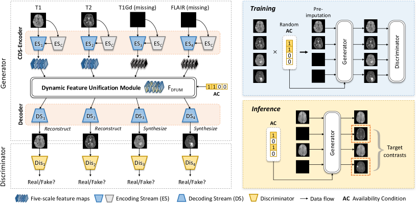
Figure 1: A schematic view of the proposed unified multi-modal image synthesis method.

Unified Synthesis: Unified synthesis receives information from any combination of available source contrasts and generates the remnant missing contrasts in a single forward pass, which is a new research point in the field of medical image synthesis. Several studies [29, 30, 1, 31] have been proposed for this scenario. For example, Chartsias et al. [29] proposed a CNN-based multi-input multi-output model, which embedded all input contrasts into a shared latent space, and transformed the latent features into the target output modality with a decoder. Sharma et al. [30] proposed an MM-GAN, which used information from all available contrasts to synthesize missing ones using a single encoding-decoding pathway. Shen et al. [1] proposed a GAN-based method with a disentanglement scheme to extract shared content encoding and separate style encoding across multiple domains. Dalmaz et al.[31] used Transformer [37] to model long-range dependencies between different modalities for unified medical image synthesis.

III Method

III-A Unified Multi-Modal Synthesis Framework

In this paper, we propose a novel unified synthesis framework for missing modality imputation from arbitrary combinations of available modalities. We mainly consider the unified synthesis task on four-modality MR sequences. However, it should be noted that our framework can be applied to multi-modal data with any number of modalities.

Fig. 1 gives a schematic view of the proposed method, which employs a generative adversarial architecture. Given randomly missing multi-modal inputs, and the Availability Conditions $AC=\{ac_{i}\in\{0,1\}\}_{i=1}^{4}$ of T1, T2, T1Gd, and FLAIR modality (with 0 denoting missing modalities, 1 denoting available modalities, $i$ denoting the $i^{th}$ modality), we pre-impute missing modalities with all-zeros [30] to ensure that the network always receives inputs with fixed four channels. In the training stage, the generator employs a Commonality- and Discrepancy-Sensitive Encoder (CDS-Encoder) to model both modality-invariant and specific information and a Dynamic Feature Unification Module (DFUM) to derive the unified latent features from input four channels, and finally decodes unified features into images of four modalities, including reconstructed images of available modalities and synthetic images of missing modalities. Subsequently, four discriminators distinguish between network-produced and real images. To ensure that the network is robust to various input configurations, the network is exposed to random missing scenario in each training iteration with a randomly generated Availability Condition. In the inference stage, the generator takes the Availability Condition and zero-imputed four channels as input, and generates images of desired missing modalities. In the following subsections, we provide further details on our method.

III-B Generator

The generator takes both available contrasts and zero-imputed missing contrasts as input and outputs images of four different modalities, which consists of the encoder, feature unification module, and decoder.

III-B1 Commonality- and Discrepancy-Sensitive Encoder

Properly encoding the effective information contained in input modalities is crucial for synthesizing images with high fidelity. Particularly, common information across all modalities guides the network to generate anatomically consistent target images, and distinct information of each modality helps the network synthesize more accurate soft tissue details (especially for tumor region synthesis). To fully exploit such two types of information, we propose a CDS-Encoder for the generator.

As depicted in Fig. 1, CDS-Encoder incorporates four modality-specific encoding streams $\{ES_{i}\}_{i=1}^{4}$ (with the same structure and individual parameters) that cope with unique characteristics of each modality, along with a common encoding stream $ES_{C}$ that copes with shared and invariant features. As the network goes deeper, two types of features are gradually combined through fusion layers \footnotesize{f}⃝ comprising a concatenation layer and a 1$\times$1 convolutional layer. Fig. 2 provides the detailed structures of $ES_{i}$ and $ES_{C}$. It should be noted that certain parameters are shared among four modality-specific encoding streams, as highlighted by the red dotted box in Fig. 2. This design serves two purposes: firstly, it recognizes that features from different modalities should be similar at high levels; secondly, it reduces the memory usage of our network considering that we use multiple streams.

With the devised encoding architecture, the input image of $i^{th}$ modality is simultaneously fed into $ES_{i}$ and $ES_{C}$ in each forward pass. As such, the common encoding stream is shared among all input images so that it can concentrate on the common information across different modalities. Finally, the CDS-Encoder outputs multi-scale features of each modality $\{{F_{i}^{(1)},F_{i}^{(2)},F_{i}^{(3)},F_{i}^{(4)},F_{i}^{(5)}}\}_{i=1}^{4}$ (i.e., four sets of five-scale features in total).

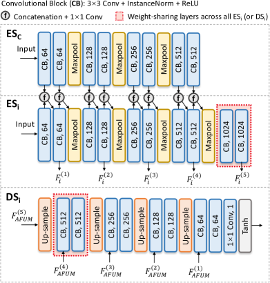
Figure 2: Illustration of the detailed structures of the common encoding stream ($ES_{C}$), modality-specific encoding stream ($ES_{i}$), and modality-specific decoding streams ($DS_{i}$).

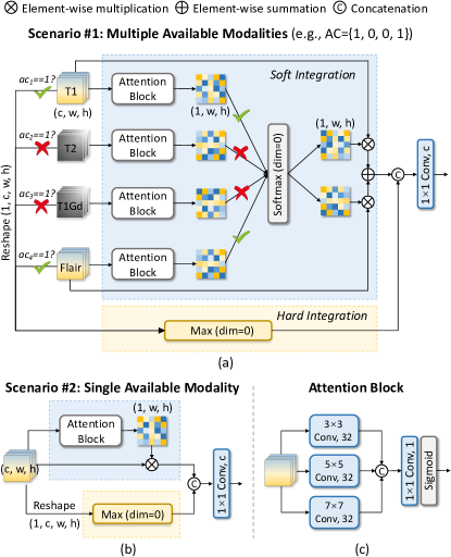
Figure 3: Illustration of the Dynamic Feature Unification Module (DFUM). (a) The scenario in which multiple modalities are available. (b) The scenario in which only a single modality is available. (c) The detailed structure of the attention block.

III-B2 Dynamic Feature Unification Module

The key challenge in unified multi-modal synthesis is how to effectively integrate latent features from a varying number of available modalities. Existing methods typically use a Max function [29] to obtain unified features that only preserve the maximum values across modalities, but this can result in a loss of valuable information (e.g., subtle structures and intensity variations present only in a subset of modalities) and negatively impact synthesis performance. To address this issue, we propose the DFUM that can dynamically integrate latent features from available modalities while retaining the unique characteristics of each modality. Fig. 3 illustrates the detailed structure of DFUM, which mainly consists of Hard Integration and Soft Integration. Given feature maps of the same scale from different modalities such as $\{F_{i}^{(1)}\}_{i=1}^{4}$ and Availability Condition $\{ac_{i}\}_{i=1}^{4}$, DFUM adaptively processes them according to various input configurations to make differential treatment and produces a unified feature $F_{DFUM}^{(1)}$.

Specifically, Fig. 3 (a) shows the scenario in which multiple modalities are available. In this scenario, Hard Integration preserves the maximum pixel value among different modalities through a Max operation, which retains the most informative features across modalities and simply discards information with low response. To enrich the representation and avoid information loss, Soft Integration employs attention mechanisms to learn the importance of each modality and weigh their pixel-wise contributions to the unified features. The used attention blocks are depicted in Fig. 3 (c), which employ convolutional layers with 3$\times$3, 5$\times$5, and 7$\times$7 kernels to compute spatial attention of each modality at different receptive fields. Noteworthy, missing modalities (with $ac_{i}=0$) are excluded from the integration process. To sum up, Hard Integration emphasizes the most important information from each modality while Soft Integration supplements some discarded features, as such, DFUM can flexibly combine features from multiple available modalities in both discrete and continuous manners. Fig. 3 (b) depicts the scenario in which only a single modality is available. In this case, Soft Integration equals a self-attention module that encourages the focus on regions-of-interest (e.g., tumor regions), and Hard Integration equals an identity function. In short, DFUM acts as a self-attention mechanism when processing a single available modality.

With this dynamic processing strategy, our DFUM facilitates both one-to-one (single modality available) and many-to-one (multiple modalities available) synthesis tasks. We plug five DFUMs in total into the generator and finally obtain five-scale unified features $\{F_{DFUM}^{(s)}\}_{s=1}^{5}$.

III-B3 Decoder

The decoder utilizes four individual decoding streams $\{DS_{i}\}_{i=1}^{4}$ to decode five-scale unified features into images of four modalities. Each decoding stream is intended for synthesizing the contrast of a specific modality. For available modalities with $ac_{i}=1$, the decoder aims to reconstruct them while for missing modalities with $ac_{i}=0$, the decoder aims to synthesize soft-tissue contrasts with desired distributions. The detailed structure of $DS_{i}$ is illustrated in Fig. 2, which progressively decodes and merges multi-scale features through sequential up-sampling and convolutional layers. Similar to the encoder, certain parameters are shared among all decoding streams (see the red dotted box in Fig. 2).

III-B4 Loss Function

We employ a hybrid loss to optimize the generator, consisting of a synthesis loss, a reconstruction loss, and an adversarial loss. Concretely, the synthesis loss $\mathcal{L}_{syn}$ is a pixel-wise L1 loss that measures the difference between synthetic images (of missing modalities) and real images:

$$\mathcal{L}_{syn}=\sum_{i=1}^{4}(1-ac_{i})\cdot L_{1}(\hat{Y}_{i},Y_{i}),$$ (1)

where $\hat{Y}_{i}$ denotes the network-produced image of the $i^{th}$ modality, $Y_{i}$ denotes the ground-truth image. $ac_{i}$ is the availability of the $i^{th}$ modality, which is randomly generated and may be different in each iteration. $(1-ac_{i})$ ensures that only missing modalities are involved.

The reconstruction loss $\mathcal{L}_{rec}$ is a pixel-wise L1 loss measuring the difference between reconstructed images (of available modalities) and real images:

$$\mathcal{L}_{rec}=\sum_{i=1}^{4}ac_{i}\cdot L_{1}(\hat{Y}_{i},Y_{i}),$$ (2)

where $ac_{i}$ ensures that only available modalities are involved.

The adversarial loss $\mathcal{L}_{adv}$ is a least square loss (L2 loss) [38] that fools the discriminators. Upon convergence, the generator produces realistic images that are indistinguishable from real images, enabling the network to better model high-frequency information and produce images that are coincident with the target distribution:

$$\mathcal{L}_{adv}=\sum_{i=1}^{4}(1-ac_{i})\cdot(L_{2}(Dis_{i}(\hat{Y}_{i})-1)+L_{2}(Dis_{i}(Y_{i}))),$$ (3)

where $Dis_{i}$ denotes the discriminator of the $i^{th}$ modality.

So far, the overall loss of the generator is formulated as:

$$\mathcal{L}_{Gen}=\lambda_{1}\mathcal{L}_{syn}+\lambda_{2}\mathcal{L}_{rec}+\lambda_{3}\mathcal{L}_{adv}.$$ (4)

where $\lambda_{1}$, $\lambda_{2}$, and $\lambda_{3}$ are trade-off parameters for each loss item. In our experiments, we achieve the best performance with $\lambda_{1}=100$, $\lambda_{2}=30$, and $\lambda_{3}=1$.

III-C Discriminator

Our network employs four discriminators $\{Dis_{i}\}_{i=1}^{4}$ to distinguish between real and synthetic images of each modality. The network structure of each discriminator follows PatchGAN [39]. Distinct from vanilla GANs that distinguish real and fake images from the whole-image level, PatchGAN conducts patch-level discrimination for input images. This can facilitate modeling local features and synthesizing realistic local details.

We use a least square loss to optimize the discriminators:

$$\mathcal{L}_{Dis}=\sum_{i=1}^{4}(1-ac_{i})\cdot(L_{2}(Dis_{i}(\hat{Y}_{i}))+L_{2}(Dis_{i}(Y_{i})-1)).$$ (5)

During training, discriminators make effort to tell apart synthetic images from real ones, which engage in adversarial training with the generator.

III-D Training Scheme

To make the network robust to any missing data scenarios when testing, we expose the network to various input configurations during training. This is achieved by masking out a subset of modalities using a random Availability Condition in each iteration as stated in Section III-A. However, since different missing data imputation tasks pose varying levels of difficulty, we introduce a Curriculum Learning [32] based training scheme. Following MM-GAN [30], we show the network easy samples (missing one contrast) for the first 10 epochs, followed by moderate samples (missing two contrasts) for the next 10 epochs, and finally hard samples (missing three contrasts) for another 10 epochs. After that, we randomly set the input scenarios for the remaining epochs. This training mechanism enables the network to efficiently learn from easier tasks and gradually adapt to harder tasks [30], which helps to improve the convergence speed and generalization ability.

Our network is implemented using Pytorch and deployed on an NVIDIA A100 GPU. We use stochastic gradient descent as the optimizer for training. The total number of training epochs is 200 and the batch size is 32. The learning rate is initially set to $2\times 10^{-4}$ for the first 50 epochs and linearly decays to zero afterward.

IV Materials and Experiments

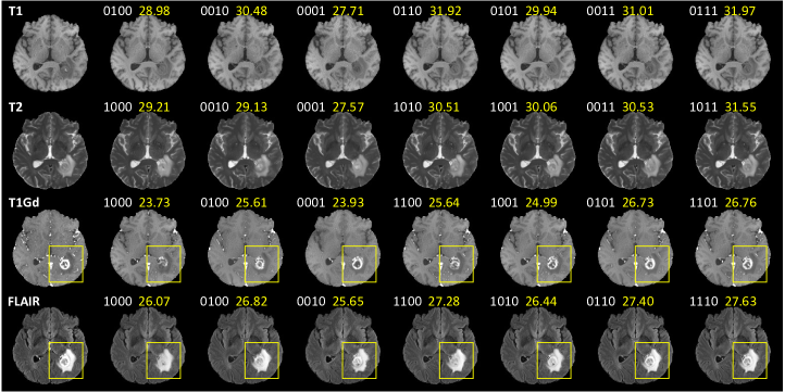
Figure 4: Visual examples of synthetic images produced by our method on the BraTS dataset. The four-bit digits represent the Availability Conditions of T1, T2, T1Gd, and FLAIR modalities, in which “0” represents the “missing” modality and “1” represents the “available” modality. Yellow boxes emphasize the obvious difference between images. The yellow decimals represent PSNR values.

IV-A Materials

To validate the effectiveness of our method, we conduct comprehensive experiments on two public multi-modal MR datasets including the BraTS 2019 dataset [33, 34, 35] and the IXI dataset (https://brain-development.org/ixi-dataset).

IV-A1 BraTS Dataset

The BraTS 2019 dataset comprises MR scans of glioblastoma and lower-grade glioma collected from 19 institutions. Each study includes skull-stripped and co-registered MR images of T1-weighted, T2-weighted, T1Gd, and FLAIR modalities. In our experiments, we randomly select 250, 20, and 20 artifact-free subjects for training, evaluation, and testing, respectively. We only use the middle 80 axial slices from each subject, which are cropped to a size of 192$\times$192 from the center region.

IV-A2 IXI Dataset

The IXI dataset comprises MR scans of healthy volunteers collected from three hospitals in London. Each study includes non-skull-stripped MR images of T1-, T2-, and PD-weighted modalities. We randomly select 170, 15, and 15 subjects for training, evaluation and testing. To prepare the images for analysis, we register the T1 and T2 volumes to the PD volumes using affine transformation (implemented through ANTsPy). For each subject, we select 60 artifact-free brain tissue slices from the middle of the image stack, which are then cropped to a size of 224$\times$224 from the center region.

TABLE I: Quantitative results of our method on the BraTS dataset.

Available modalities				Results [mean PSNR (std), mean SSIM (std)]
T1	T2	T1Gd	FLAIR	T1	T2	T1Gd	FLAIR
			✓	27.38 (1.29), 0.938 (0.013)	26.52 (1.22), 0.924 (0.021)	24.65 (0.99), 0.883 (0.024)	-
		✓		31.09 (1.84), 0.969 (0.020)	27.66 (1.08), 0.941 (0.017)	-	25.52 (1.12), 0.882 (0.024)
	✓			28.88 (1.38), 0.958 (0.018)	-	25.96 (0.94), 0.915 (0.024)	26.81 (1.56), 0.903 (0.028)
✓				-	27.78 (1.16), 0.944 (0.017)	26.57 (1.47), 0.921 (0.030)	25.94 (1.08), 0.891 (0.023)
		✓	✓	31.47 (1.80), 0.972 (0.017)	28.78 (1.27), 0.954 (0.014)	-	-
	✓		✓	29.47 (1.28), 0.963 (0.013)	-	26.55 (1.11), 0.923 (0.023)	-
✓			✓	-	28.68 (1.29), 0.954 (0.014)	27.08 (1.41), 0.928 (0.028)	-
	✓	✓		31.86 (2.03), 0.974 (0.019)	-	-	27.16 (1.60), 0.911 (0.026)
✓		✓		-	28.48 (1.14), 0.952 (0.015)	-	26.22 (1.21), 0.898 (0.023)
✓	✓			-	-	27.68 (1.49), 0.938 (0.025)	27.32 (1.57), 0.913 (0.026)
	✓	✓	✓	31.94 (1.94), 0.975 (0.017)	-	-	-
✓		✓	✓	-	29.28 (1.28), 0.959 (0.013)	-	-
✓	✓		✓	-	-	27.93 (1.51), 0.940 (0.025)	-
✓	✓	✓		-	-	-	27.39 (1.59), 0.915 (0.026)

In this study, both two datasets are normalized using mean normalization to ensure comparable ranges of voxel intensities across subjects.

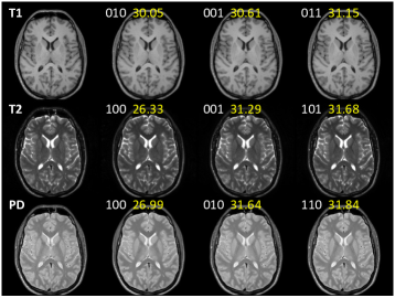
Figure 5: Visual examples of synthetic images produced by our method on the IXI dataset. The three-bit digits represent the Availability Conditions of T1, T2, and PD modalities, in which “0” represents “missing” modality and “1” represents “available” modality. The yellow decimals represent PSNR values.

IV-B Competing Methods and Evaluation Metrics

To demonstrate the superiority of our method, we compare it with state-of-the-art methods in various synthesis tasks. Specifically, in the one-to-one synthesis scenario, two competing methods are considered: pGAN [16] and Pix2Pix [39]; In the many-to-one synthesis scenario, Hi-Net [24] is considered as the competing method; Finally, in the unified synthesis scenario, we consider two competing methods: MM-Synthesis [29] and MM-GAN [30]. Note that MM-GAN is reproduced strictly according to its paper while other comparison methods are implemented using open-source codes.

To quantitatively assess the performance of synthesis methods, we adopt two commonly-used evaluation metrics: peak signal-to-noise ratio (PSNR) and structural similarity index (SSIM). Given a synthetic volume $\hat{y}$ and the ground-truth volume $y$, PSNR is defined as: $PSNR(\hat{y},y)=10log_{10}{\frac{max^{2}(\hat{y},y)}{|\Omega|^{-1}\sum\left\|\hat{y}-y\right\|_{2}^{2}}}$, where $|\Omega|$ is the voxel numbers of $y$, $max^{2}(\hat{y},y)$ is the maximal intensity value of $\hat{y}$ and $y$. SSIM is defined as: $SSIM(\hat{y},y)=\frac{(2\mu_{\hat{y}}\mu_{y}+c_{1})(2\sigma_{\hat{y}y}+c_{2})}{(\mu_{\hat{y}}^{2}+\mu_{y}^{2}+c_{1})(\sigma_{\hat{y}}^{2}+\sigma_{y}^{2}+c_{2})}$, where $\mu_{y}$, $\sigma_{y}$ is the mean and variance of $y$, $\sigma_{\hat{y}y}$ is the covariance between $\hat{y}$ and $y$. The higher value of PSNR and SSIM indicates better image quality. Besides, we calculate the $p$-value using a two-sample $t$-test to assess the statistical significance of our method in comparison to other methods.

TABLE II: Quantitative results of our method on the IXI dataset.

Available modalities			Results [mean PSNR (std), mean SSIM (std)]
T1	T2	PD	T1	T2	PD
		✓	29.31 (0.53), 0.969 (0.005)	30.93 (0.48), 0.943 (0.027)	-
	✓		28.48 (0.51), 0.964 (0.007)	-	31.07 (0.46), 0.977 (0.004)
✓			-	26.43 (0.39), 0.911 (0.026)	26.96 (0.48), 0.950 (0.008)
	✓	✓	29.50 (0.51), 0.971 (0.006)	-	-
✓		✓	-	31.32 (0.49), 0.948 (0.025)	-
✓	✓		-	-	31.86 (0.41), 0.980 (0.004)

IV-C Results of the Proposed Method

In Fig. 4 and Fig. 5, we present examples of synthetic images produced by our method on the BraTS and IXI datasets. The four-bit (or three-bit) digits in the figures indicate the Availability Conditions of T1, T2, T1Gd, and FLAIR modalities (or T1, T2, and PD modalities), with “1” representing available modality and “0” representing missing modality. Our results demonstrate that synthesizing a target contrast using more available contrasts produces images with better quality. The combination of complementary information from multiple modalities is particularly crucial for synthesizing tumor regions with accurate shapes and realistic textures. For example, when synthesizing T1Gd images with glioblastoma (see the third row in Fig. 4), using only T1 information leads to unsatisfactory results with incomplete and improperly enhanced tumor regions. However, extra combining T2 or FLAIR information greatly improves the synthesis quality as these two modalities provide clear demarcation of tumors. Table I and Table II present the quantitative results of our method with different input-output configurations on the two datasets. The tables show that synthesizing the target modality using the largest number of available modalities achieves the best performance as measured by PSNR and SSIM, which is consistent with the qualitative results.

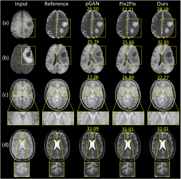
Figure 6: Visual examples of comparison results in one-to-one synthesis tasks on two datasets: (a) T1$\rightarrow$T2 and (b) FLAIR$\rightarrow$T1 in the BraTS dataset; (c) T1$\rightarrow$PD and (d) PD$\rightarrow$T2 in the IXI dataset. Yellow boxes emphasize distinctions between images, in which regions with subtle differences are enlarged for a better view. The yellow decimals represent PSNR values.

IV-D Comparison with State-of-the-Art Methods

Our proposed unified synthesis method is capable of handling synthesis tasks with various input-output configurations. In this section, we specifically compare our method with state-of-the-art methods in one-to-one, many-to-one, and unified synthesis tasks, respectively.

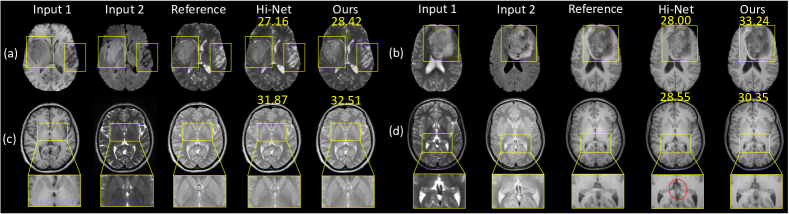
Figure 7: Visual examples of comparison results in many-to-one synthesis tasks on two datasets: (a) T1+FLAIR$\rightarrow$T2 and (b) T2+FLAIR$\rightarrow$T1 in the BraTS dataset; (c) T1+T2$\rightarrow$PD and (d) T2+PD$\rightarrow$T1 in the IXI dataset. Yellow boxes emphasize distinctions between images, in which regions with subtle differences are enlarged for a better view, the red ellipse emphasizes the streaking noises, and the yellow decimals represent PSNR values.

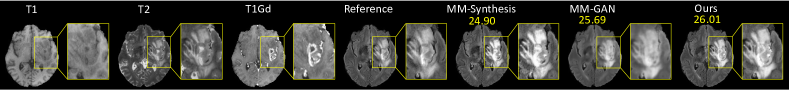
Figure 8: Representative examples (T1+T2+T1Gd$\rightarrow$FLAIR) of unified synthesis on the BraTS dataset. Yellow boxes emphasize distinctions between images, which are enlarged for a better view, and the yellow decimals represent PSNR values.

TABLE III: Quantitative comparison with one-to-one synthesis methods in various tasks on the BraTS dataset (T1$\rightarrow$T2 and FLAIR$\rightarrow$T1) and IXI dataset (T1$\rightarrow$PD and PD$\rightarrow$T2) ($p$¡0.05).

	Results [mean PSNR (std), mean SSIM (std)]
	T1$\rightarrow$T2	FLAIR$\rightarrow$T1	T1$\rightarrow$PD	PD$\rightarrow$T2
pGAN	27.10 (1.28), 0.933 (0.019)	26.91 (1.28), 0.932 (0.016)	26.42 (0.44), 0.942 (0.009)	30.30 (0.63), 0.935 (0.034)
Pix2Pix	26.94 (1.28), 0.931 (0.019)	26.86 (1.33), 0.931 (0.017)	26.01 (0.47), 0.938 (0.010)	29.94 (0.45), 0.943 (0.019)
Ours	27.78 (1.16), 0.944 (0.017)	27.38 (1.29), 0.938 (0.013)	26.96 (0.48), 0.950 (0.008)	30.93 (0.48), 0.943 (0.027)

TABLE IV: Quantitative comparison with many-to-one synthesis methods in various tasks on the BraTS dataset (T1+FLAIR$\rightarrow$T2 and T2+FLAIR$\rightarrow$T1) and IXI dataset (T1+T2$\rightarrow$PD and T2+PD$\rightarrow$T1) ($p$¡0.05).

	Results [mean PSNR (std), mean SSIM (std)]
	T1+FLAIR$\rightarrow$T2	T2+FLAIR$\rightarrow$T1	T1+T2$\rightarrow$PD	T2+PD$\rightarrow$T1
Hi-Net	27.24 (1.33), 0.929 (0.020)	27.25 (1.62), 0.925 (0.030)	30.08 (1.54), 0.967 (0.018)	27.85 (1.12), 0.954 (0.021)
Ours	28.68 (1.29), 0.954 (0.014)	29.47 (1.28), 0.963 (0.013)	31.86 (0.41), 0.980 (0.004)	29.50 (0.51), 0.971 (0.006)

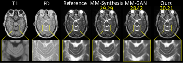
Figure 9: Representative examples (T1+PD$\rightarrow$T2) of unified synthesis on the IXI dataset. Yellow boxes emphasize distinctions between images, which are enlarged for a better view, and the yellow decimals represent PSNR values.

IV-D1 One-to-One Synthesis

For the one-to-one synthesis scenario, two representative synthesis tasks in the BraTS dataset are considered: T1$\rightarrow$T2 and FLAIR$\rightarrow$T1, and another two tasks in the IXI dataset are considered: T1$\rightarrow$PD and PD$\rightarrow$T2. Fig. 6 gives visual examples of the comparison results. It is shown that our method generates images with the most accurate tumor morphology (see Fig. 6 (a) and (b)) and subtle structural information (see Fig. 6 (c) and (d)). The improvements can be attributed to two points. First, for a single available modality, our DFUM equals a self-attention module, allowing the network to focus on critical regions (e.g., tumor regions) and suppress redundant information. Second, instead of learning a single mapping between a fixed single input and output like pGAN and Pix2Pix, our method takes a unified learning framework that learns mappings between input and output modalities of various synthesis tasks, and different tasks facilitate each other during training. Take the T1$\rightarrow$T2 task as an example, the related encoding streams $ES_{1}$, $ES_{C}$, and decoding stream $DS_{2}$ are also refined and updated by other tasks including T1$\rightarrow$T1Gd, T1$\rightarrow$FLAIR, T1Gd$\rightarrow$T2, FLAIR$\rightarrow$T2, etc. This makes the network more robust and avoids trapping into a local optimum. Table III gives the quantitative results of the comparison. Our method outperforms pGAN and Pix2Pix in PSNR and SSIM in all tasks ($p<$0.05). Both qualitative and quantitative results suggest the superiority of the proposed method.

TABLE V: Quantitative comparison results of our method and other unified synthesis methods on the BraTS dataset ($p$¡0.05).

Available modalities				Results [mean PSNR (std), mean SSIM (std)]
T1	T2	T1Gd	FLAIR	MM-Synthesis	MM-GAN	Ours
			✓	25.30 (1.13), 0.895 (0.026)	25.17 (1.15), 0.896 (0.028)	26.18 (1.14), 0.915 (0.023)
		✓		27.22 (2.11), 0.917 (0.040)	27.04 (2.40), 0.914 (0.046)	28.09 (2.29), 0.931 (0.036)
	✓			26.25 (1.37), 0.907 (0.031)	26.01 (1.23), 0.908 (0.027)	27.22 (1.23), 0.925 (0.024)
✓				25.96 (0.71), 0.901 (0.024)	25.79 (0.82), 0.900 (0.028)	26.76 (0.76), 0.919 (0.022)
		✓	✓	28.61 (1.62), 0.946 (0.016)	29.02 (1.59), 0.954 (0.013)	30.12 (1.34), 0.963 (0.009)
	✓		✓	26.72 (1.72), 0.924 (0.029)	26.56 (1.42), 0.927 (0.024)	28.01 (1.46), 0.943 (0.020)
✓			✓	26.34 (0.64), 0.917 (0.013)	26.86 (0.69), 0.928 (0.014)	27.88 (0.80), 0.941 (0.013)
	✓	✓		28.20 (2.35), 0.924 (0.042)	28.68 (2.31), 0.934 (0.036)	29.51 (2.35), 0.942 (0.031)
✓		✓		26.30 (0.94), 0.904 (0.030)	26.25 (1.17), 0.907 (0.034)	27.35 (1.13), 0.925 (0.027)
✓	✓			25.91 (0.02), 0.896 (0.014)	26.58 (0.05), 0.912 (0.013)	27.50 (0.18), 0.926 (0.012)
	✓	✓	✓	30.60 (1.55), 0.967 (0.016)	31.06 (1.65), 0.970 (0.015)	31.94 (1.94), 0.975 (0.017)
✓		✓	✓	27.36 (1.27), 0.936 (0.019)	28.12 (1.12), 0.950 (0.013)	29.28 (1.28), 0.959 (0.013)
✓	✓		✓	25.94 (1.16), 0.910 (0.023)	26.88 (1.32), 0.928 (0.024)	27.93 (1.51), 0.940 (0.025)
✓	✓	✓		25.87 (1.22), 0.883 (0.026)	26.64 (1.45), 0.902 (0.025)	27.39 (1.59), 0.915 (0.026)

TABLE VI: Quantitative comparison results of our method and other unified synthesis methods on the IXI dataset ($p$¡0.05).

Available modalities			Results [mean PSNR (std), mean SSIM (std)]
T1	T2	PD	MM-Synthesis	MM-GAN	Ours
		✓	28.99 (0.33), 0.946 (0.016)	28.86 (0.85), 0.948 (0.008)	30.12 (0.81), 0.956 (0.013)
	✓		28.56 (0.74), 0.962 (0.006)	28.48 (1.35), 0.958 (0.011)	29.78 (1.30), 0.970 (0.007)
✓			25.58 (0.39), 0.913 (0.024)	25.77 (0.38), 0.912 (0.025)	26.70 (0.27), 0.930 (0.019)
	✓	✓	28.74 (0.71), 0.964 (0.008)	28.32 (0.67), 0.961 (0.007)	29.50 (0.51), 0.971 (0.006)
✓		✓	29.51 (0.58), 0.932 (0.030)	30.01 (0.56), 0.943 (0.016)	31.32 (0.49), 0.948 (0.025)
✓	✓		29.55 (0.52), 0.969 (0.005)	30.56 (0.47), 0.973 (0.005)	31.86 (0.41), 0.980 (0.004)

IV-D2 Many-to-One Synthesis

For the many-to-one synthesis scenario, two representative synthesis tasks in the BraTS dataset are considered: T1+FLAIR$\rightarrow$T2 and T2+FLAIR$\rightarrow$T1. Meanwhile, in the IXI dataset, another two many-to-one tasks are considered: T1+T2$\rightarrow$PD and T2+PD$\rightarrow$T1. As shown in Fig. 7, synthetic images produced by Hi-Net are more blurry and lose certain high-frequency details (see Fig. 7 (a) and (c)). Besides, in Fig. 7 (d), Hi-Net does not combine information from multiple modalities effectively and produces streaking noises (emphasized by the red ellipse in Fig. 7). Compared with Hi-Net, our method generates more visually pleasing images. In addition to the advantage of the unified learning framework (explained in Section IV-D1), our method also benefits from the multi-modal feature integration strategy of DFUM, which aggregates features through both hard (discrete) and soft (continuous) combination. As such, DFUM ensures the effective fusion of features while avoiding the loss of valuable information contained in each modality. Table III presents the quantitative comparison results between our method and Hi-Net in four many-to-one synthesis tasks on the BraTS dataset and IXI dataset. It is shown that our method outperforms Hi-Net in both PSNR and SSIM for all tasks ($p<$0.05), implying that the proposed method has superior performance.

IV-D3 Unified Synthesis

For the unified synthesis scenario, we compare our method with MM-Synthesis [29] and MM-GAN [30] with all possible combinations of inputs on two datasets. Concretely, 14 input scenarios are investigated in the BraTS dataset and 6 input scenarios are investigated in the IXI dataset. Table V and Table VI summarize the comparison results. The numerical result of each input scenario is averaged on all generated missing modalities. It is demonstrated that the proposed method achieves better values than competing methods in both PSNR and SSIM metrics ($p<$0.05) in different input scenarios. To show visual examples of the comparison, we select two representative synthesis tasks, including (1) T1+T2+T1Gd$\rightarrow$FLAIR in the BraTS dataset, and (2) T1+PD$\rightarrow$T2 in the IXI dataset, and display the synthesized results in Fig. 8 and Fig. 9. It is observed that MM-Synthesis may generate excessive contrast for the tumor region (see Fig. 8) or lose certain structural information (see Fig. 9). The reason may be that MM-Synthesis is a CNN-based synthesis method that does not use the adversarial loss to constrain the local structure and high-frequency characteristics of the synthetic images. In addition, MM-Synthesis only retains the maximum response value when merging multi-modal features, but the source modality with the highest response value does not necessarily provide sufficient detailed information for the target modality. MM-GAN tends to produce blurry images that lack rich details (see Fig. 8 and Fig. 9). The reason may be that in MM-GAN, different input modalities are processed by a single encoding and decoding pathway. This makes the network better at mining modality-invariant features, but less sensitive to modality-specific details, thereby limiting the quality of the generated images. In comparison, our method synthesizes images with the highest quality, because we use a more reasonable multi-modal feature integration strategy and employ both modality-shared and modality-specific streams to comprehensively analyze the information from input contrasts.

IV-E Ablation Study

In this section, we validate the effectiveness of each newly proposed component in our method.

IV-E1 The Rationality of the CDS-Encoder

First, we examine the structural rationality of the CDS-Encoder proposed in our work. To highlight the benefits of our encoding method, we compare it with two other encoding approaches: (1) MMS-Encoder, which employs multiple modality-specific encoding streams, with each stream corresponding to an input modality, and (2) C-Encoder, which uses a single common encoding stream to handle all possible input modalities. Table VII displays the quantitative comparison results, where all variants have the same network structure except for the encoder. We report the average numerical results of each method across 14 input scenarios on the BraTS dataset. It is shown that the CDS-Encoder achieves 28.23 dB in PSNR and 0.937 in SSIM, outperforming the MMS-Encoder by +0.40 dB in PSNR and +0.006 in SSIM, and C-Encoder by +0.98 dB in PSNR and +0.012 in SSIM. These superior results demonstrate that our proposed CDS-Encoder is both rational and effective for processing multi-modal inputs.

TABLE VII: Ablation study on the BraTS dataset. All results are averaged across 14 input scenarios.

Experiments	PSNR	SSIM
MMS-Encoder	27.83 (1.45)	0.931 (0.019)
C-Encoder	27.25 (0.57)	0.925 (0.010)
CDS-Encoder (ours)	28.23 (1.46)	0.937 (0.018)
Max operation	27.79 (1.10)	0.932 (0.015)
HeMIS	27.60 (0.93)	0.930 (0.013)
DFUM (ours)	28.23 (1.46)	0.937 (0.018)
Ours w/o CL	27.93 (1.48)	0.933 (0.018)
Ours w/ CL	28.23 (1.46)	0.937 (0.018)

IV-E2 The Effectiveness of DFUM

In this work, we propose a feature unification strategy (the DFUM) to prepare unified latent features for the decoding stage, which consists of soft feature integration and hard feature integration. Here, we demonstrate the superiority of DFUM by comparing it with known feature unification strategies: (1) Max operation [29], which only retains the maximum value of input multi-modal features at spatial positions, and (2) HeMIS [40], which computes the mean and variance of input multi-modal features. Table VII shows the quantitative comparison results on the BraTS dataset. From the table, the proposed DFUM outperforms Max operation by +0.44 dB in PSNR and +0.005 in SSIM, and HeMIS by +0.63 dB in PSNR and +0.007 in SSIM, indicating that DFUM can most effectively combine features from available modalities.

IV-E3 The Effectiveness of Curriculum Learning

As mentioned in Section III-D, we utilize a curriculum learning (CL) strategy during training to allow the network to learn synthetic tasks from easy to difficult. Here, we verify the effectiveness of this training scheme by conducting two experiments: “Ours w/ CL” which incorporates the CL scheme in the training, and “Ours w/o CL” which does not use the CL strategy, and exposes the network to random Availability Conditions at all times. The results in Table VII indicate that incorporating CL increases the performance by +0.30 dB in PSNR and +0.004 in SSIM, demonstrating the effectiveness of the CL training scheme.

V Conclusion

In this paper, we present a novel approach for unified multi-modal image synthesis using a generative adversarial network. To fully exploit the commonality and discrepancy information of available modalities, we introduce a Commonality- and Discrepancy-Sensitive Encoder for the generator that analyses both modality-invariant and modality-specific information, respectively. Besides, we devise a Dynamic Feature Unification Module that can effectively derive the unified features from a varying number of available modalities. Despite its impressive results as shown in Section IV, the proposed method has certain limitations. One such limitation arises from the use of multiple encoding and decoding streams in the network, which leads to potential memory consumption issues when extending the framework to more modalities. Therefore, a more lightweight and memory-efficient network architecture is needed to accommodate additional modalities in the future.

References

- [1] L. Shen et al., “Multi-domain image completion for random missing input data,” IEEE TMI, vol. 40, no. 4, pp. 1113–1122, 2020.
- [2] I. Goodfellow et al., “Generative adversarial networks,” Communications of the ACM, vol. 63, no. 11, pp. 139–144, 2020.
- [3] Bowles et al., “Pseudo-healthy image synthesis for white matter lesion segmentation,” in Simulation and Synthesis in Medical Imaging: First International Workshop, Proceedings 1. Springer, 2016, pp. 87–96.
- [4] S. Roy, Y.-Y. Chou, A. Jog, J. A. Butman, and D. L. Pham, “Patch based synthesis of whole head mr images: Application to epi distortion correction,” in Simulation and Synthesis in Medical Imaging: First International Workshop, Proceedings 1. Springer, 2016, pp. 146–156.
- [5] S. Roy, A. Carass, and J. L. Prince, “Magnetic resonance image example-based contrast synthesis,” IEEE TMI, vol. 32, no. 12, pp. 2348–2363, 2013.
- [6] Y. Huang, L. Beltrachini, L. Shao, and A. F. Frangi, “Geometry regularized joint dictionary learning for cross-modality image synthesis in magnetic resonance imaging,” in Simulation and Synthesis in Medical Imaging: First International Workshop. Springer, 2016, pp. 118–126.
- [7] A. Jog, A. Carass, S. Roy, D. L. Pham, and J. L. Prince, “Mr image synthesis by contrast learning on neighborhood ensembles,” Medical image analysis, vol. 24, no. 1, pp. 63–76, 2015.
- [8] D. H. Ye, D. Zikic, B. Glocker, A. Criminisi, and E. Konukoglu, “Modality propagation: coherent synthesis of subject-specific scans with data-driven regularization,” in MICCAI, Part I 16. Springer, 2013, pp. 606–613.
- [9] R. Vemulapalli, H. Van Nguyen, and S. K. Zhou, “Unsupervised cross-modal synthesis of subject-specific scans,” in ICCV, 2015, pp. 630–638.
- [10] H. Van Nguyen, K. Zhou, and R. Vemulapalli, “Cross-domain synthesis of medical images using efficient location-sensitive deep network,” in MICCAI 2015, Proceedings, Part I 18. Springer, 2015, pp. 677–684.
- [11] V. Sevetlidis, M. V. Giuffrida, and S. A. Tsaftaris, “Whole image synthesis using a deep encoder-decoder network,” in Simulation and Synthesis in Medical Imaging: First International Workshop, Proceedings 1. Springer, 2016, pp. 127–137.
- [12] R. Li et al., “Deep learning based imaging data completion for improved brain disease diagnosis,” in MICCAI, Part III 17. Springer, 2014, pp. 305–312.
- [13] D. Nie et al., “Medical image synthesis with context-aware generative adversarial networks,” in MICCAI, Part III 20. Springer, 2017, pp. 417–425.
- [14] ——, “Medical image synthesis with deep convolutional adversarial networks,” IEEE TBME, vol. 65, no. 12, pp. 2720–2730, 2018.
- [15] Q. Wang et al., “Realistic lung nodule synthesis with multi-target co-guided adversarial mechanism,” IEEE TMI, vol. 40, no. 9, pp. 2343–2353, 2021.
- [16] S. U. Dar et al., “Image synthesis in multi-contrast mri with conditional generative adversarial networks,” IEEE TMI, vol. 38, no. 10, pp. 2375–2388, 2019.
- [17] W. Yuan, J. Wei, J. Wang, Q. Ma, and T. Tasdizen, “Unified generative adversarial networks for multimodal segmentation from unpaired 3d medical images,” Medical Image Analysis, vol. 64, p. 101731, 2020.
- [18] Y. Luo et al., “Adaptive rectification based adversarial network with spectrum constraint for high-quality pet image synthesis,” Medical Image Analysis, vol. 77, p. 102335, 2022.
- [19] Y. Fei, C. Zu, Z. Jiao, X. Wu, J. Zhou, D. Shen, and Y. Wang, “Classification-aided high-quality pet image synthesis via bidirectional contrastive gan with shared information maximization,” in MICCAI, Part VI. Springer, 2022, pp. 527–537.
- [20] A. Jog et al., “Random forest flair reconstruction from t 1, t 2, and p d-weighted mri,” in ISBI. IEEE, 2014, pp. 1079–1082.
- [21] ——, “Random forest regression for magnetic resonance image synthesis,” Medical image analysis, vol. 35, pp. 475–488, 2017.
- [22] D. Lee, J. Kim, W.-J. Moon, and J. C. Ye, “Collagan: Collaborative gan for missing image data imputation,” in CVPR, 2019, pp. 2487–2496.
- [23] H. Li et al., “Diamondgan: unified multi-modal generative adversarial networks for mri sequences synthesis,” in MICCAI, Part IV 22. Springer, 2019, pp. 795–803.
- [24] T. Zhou, H. Fu, G. Chen, J. Shen, and L. Shao, “Hi-net: hybrid-fusion network for multi-modal mr image synthesis,” IEEE TMI, vol. 39, no. 9, pp. 2772–2781, 2020.
- [25] B. Peng, B. Liu, Y. Bin, L. Shen, and J. Lei, “Multi-modality mr image synthesis via confidence-guided aggregation and cross-modality refinement,” IEEE J-BHI, vol. 26, no. 1, pp. 27–35, 2021.
- [26] S. Olut, Y. H. Sahin, U. Demir, and G. Unal, “Generative adversarial training for mra image synthesis using multi-contrast mri,” in PRedictive Intelligence in MEdicine: First International Workshop, Proceedings 1. Springer, 2018, pp. 147–154.
- [27] X. Yang et al., “Bi-modality medical image synthesis using semi-supervised sequential generative adversarial networks,” IEEE J-BHI, vol. 24, no. 3, pp. 855–865, 2019.
- [28] Hagiwara et al., “Improving the quality of synthetic flair images with deep learning using a conditional generative adversarial network for pixel-by-pixel image translation,” American journal of neuroradiology, vol. 40, no. 2, pp. 224–230, 2019.
- [29] A. Chartsias, T. Joyce, M. V. Giuffrida, and S. A. Tsaftaris, “Multimodal mr synthesis via modality-invariant latent representation,” IEEE TMI, vol. 37, no. 3, pp. 803–814, 2017.
- [30] A. Sharma and G. Hamarneh, “Missing mri pulse sequence synthesis using multi-modal generative adversarial network,” IEEE TMI, vol. 39, no. 4, pp. 1170–1183, 2019.
- [31] O. Dalmaz, M. Yurt, and T. Çukur, “Resvit: residual vision transformers for multimodal medical image synthesis,” IEEE TMI, vol. 41, no. 10, pp. 2598–2614, 2022.
- [32] Y. Bengio, J. Louradour, R. Collobert, and J. Weston, “Curriculum learning,” in ICML, 2009, pp. 41–48.
- [33] S. Bakas et al., “Advancing the cancer genome atlas glioma mri collections with expert segmentation labels and radiomic features,” Scientific data, vol. 4, no. 1, pp. 1–13, 2017.
- [34] B. H. Menze et al., “The multimodal brain tumor image segmentation benchmark (brats),” IEEE TMI, vol. 34, no. 10, pp. 1993–2024, 2014.
- [35] S. Bakas et al., “Identifying the best machine learning algorithms for brain tumor segmentation, progression assessment, and overall survival prediction in the brats challenge,” arXiv preprint arXiv:1811.02629, 2018.
- [36] M. Yurt et al., “mustgan: multi-stream generative adversarial networks for mr image synthesis,” Medical image analysis, vol. 70, p. 101944, 2021.
- [37] K. Han et al., “A survey on vision transformer,” IEEE TPAMI, vol. 45, no. 1, pp. 87–110, 2022.
- [38] X. Mao et al., “Least squares generative adversarial networks,” in ICCV, 2017, pp. 2794–2802.
- [39] P. Isola, J.-Y. Zhu, T. Zhou, and A. A. Efros, “Image-to-image translation with conditional adversarial networks,” in CVPR, 2017, pp. 1125–1134.
- [40] M. Havaei, N. Guizard, N. Chapados, and Y. Bengio, “Hemis: Hetero-modal image segmentation,” in MICCAI, Part II 19. Springer, 2016, pp. 469–477.