An extremal problem and inequalities for entire functions of exponential type

Abstract.

We study two variations of the classical one-delta problem for entire functions of exponential type, known also as the Carathéodory–Fejér–Turán problem. The first variation imposes the additional requirement that the function is radially decreasing while the second one is a generalization which involves derivatives of the entire function. Various interesting inequalities, inspired by results due to Duffin and Schaeffer, Landau, and Hardy and Littlewood, are also established.

1. Introduction

In the present note we study some extremal problems concerning certain quantities over specific families of entire functions of exponential type. For $\Delta>0$, we say that an entire function $G:\mathbb{C}\to\mathbb{C}$ has exponential type at most $2\pi\Delta$ if, for all $\varepsilon>0$, there exists a positive constant $C_{\varepsilon}$ such that

$$|G(z)|\leq C_{\varepsilon}\,e^{(2\pi\Delta+\varepsilon)|z|},\,\,\,\,\,\,\mbox{for all}\,\,\,\,z\in\mathbb{C}.$$

We adopt the usual convention that an entire function $f:\mathbb{C}\to\mathbb{C}$ is said to be real if its restriction to $\mathbb{R}$ is real-valued, as well as, that the function $g^{*}(z)$ is defined by $g^{*}(z)=\overline{g(\overline{z})}$. For $f,g\in L^{1}(\mathbb{R})$ we denote by $f\ast g$ their convolution, which is defined by $(f\ast g)(x)=\displaystyle\int_{-\infty}^{\infty}f(y)g(x-y)\,\text{\rm d}y$.

1.1. The one-delta problem

The classical one-delta problem is to determine the infimum

$$\mathcal{A}=\inf_{\begin{subarray}{c}g\in\mathcal{G}\end{subarray}}{\int_{-\infty}^{\infty}g(x)\,\text{\rm d}x},$$

where the class $\mathcal{G}$ consists of real entire functions $g:\mathbb{C}\to\mathbb{C}$ of exponential type at most $2\pi$ which are majorants of a one-delta function at the origin over the real line, i.e, $g(x)\geq 0$ for all $x\in\mathbb{R}$ and $g(0)\geq 1$. By scaling, this is equivalent

$$\mathcal{A}=\inf_{\begin{subarray}{c}f\in\mathcal{F}\\ f(0)\neq 0\end{subarray}}\dfrac{\|f\|_{1}}{f(0)},$$

where the family $\mathcal{F}$ consists of real entire functions $f:\mathbb{C}\to\mathbb{C}$ of exponential type at most $2\pi$ such that $f\in L^{1}(\mathbb{R})$, and $f(x)\geq 0$ for all $x\in\mathbb{R}$. This is a classical problem, and several of its variations are named after Carathéodory, Fejér and Turán. We refer to [10, 12, 20, 23] for comprehensive information about its history and for some recent contributions. It is known that $\mathcal{A}=1$, and the unique extremal solution of the one-delta problem is the Fejér kernel, given by

$$K(z)=\Big{(}\dfrac{\sin\pi z}{\pi z}\Big{)}^{2}.$$ (1.1)

To obtain an equivalent formulation of this problem, we may consider a decomposition result due to Krein [1, p. 154]. It states that if $f:\mathbb{C}\to\mathbb{C}$ is an entire function of exponential type at most $2\pi$ such that $f\in L^{1}(\mathbb{R})$ and $f(x)\geq 0$ for all $x\in\mathbb{R}$, then there exists an entire function $g:\mathbb{C}\to\mathbb{C}$ in the Paley–Wiener space $PW^{2}$ such that $f(z)=g(z)g^{*}(z)$. Here, $PW^{2}$ is the subspace of $L^{2}(\mathbb{R})$ consisting of entire functions of exponential type at most $\pi$. Therefore, the one-delta problem can also be stated as finding

$$\mathcal{A}=\inf_{\begin{subarray}{c}g\in PW^{2}\\ g(0)\neq 0\end{subarray}}\dfrac{\|g\|^{2}_{2}}{|g(0)|^{2}}.$$ (1.2)

Other $L^{p}-$variations of this problem have also been studied in [4, 7, 19]. Note that (1.2) can be stated in yet another alternative way as follows: the inequality

$$1\leq\int_{-\infty}^{\infty}|g(x)|^{2}\,\text{\rm d}x,$$ (1.3)

holds for every $g\in PW^{2}$ such that $g(0)=1$, and (1.3) reduces to an equality if and only if

$$g(z)=\dfrac{\sin\pi z}{\pi z}.$$

Our main goal is to study some natural variations of each of the above versions of the one-delta problem.

1.2. Monotone-delta problem

The monotone-delta problem is to find

$$\mathcal{A}_{1}=\inf_{\begin{subarray}{c}f\in\mathcal{F}_{1}\\ f(0)\neq 0\end{subarray}}\dfrac{\|f\|_{1}}{f(0)},$$ (1.4)

where the family $\mathcal{F}_{1}$ consists of real entire functions $f:\mathbb{C}\to\mathbb{C}$ of exponential type at most $2\pi$, such that $f\in L^{1}(\mathbb{R})$, $f(x)\geq 0$ for all $x\in\mathbb{R}$, and $f$ is radially decreasing, that is, $f$ is increasing on $(-\infty,0)$ and decreasing on $(0,\infty)$. To the best of our knowledge, this problem was posed explicitly by Jeffrey Vaaler. It is a variant, with additional constraints, of another problem, solved by Holt and Vaaler in [16]. Another minimization problem with monotonicity restrictions was considered in [6] by Carneiro and Littmann, in the setting of one-sided majorants for the signum function.

In the following theorem, we present some qualitative and quantitative information about this problem.

Theorem 1.

The following statements about the monotone-delta problem hold:

• There exists an even function $F\in\mathcal{F}_{1}$ with $F(0)=1$ that extremizes (1.4).

• All the zeros of any even extremizer $F$ lie in the set $S=\{z\in\mathbb{C}:|{\rm Re}\,{z}|>|{\rm Im}\,{z}|>0\}.$

• The constant $\mathcal{A}_{1}$ satisfies $1.2750<\mathcal{A}_{1}<1.27714.$

Part (a) follows from standard compactness arguments. For part (b) we will show that zeros outside of $\mathcal{S}$ will either force a function to be zero, by analytic continuation and the constraints in the class $\mathcal{F}_{1}$, or one can carefully remove said zero and arrive at a contradiction. Part (c) of Theorem 1 is constructive, and although our lower bound only coincides up the two first digits, we conjecture that the upper bound in part (c) is sharp, at least up the first four significant digits of $\mathcal{A}_{1}$ shown above. As evidence, we exhibit concrete examples for which the value 1.2771…is attained. To estimate $\mathcal{A}_{1}$, we first reformulate the monotone-delta problem (see Lemma 6 below) to the one of determining the infimum

$$\mathcal{A}_{1}=\inf_{\begin{subarray}{c}h\in\mathcal{F}_{2}\\ h\not\equiv 0\end{subarray}}\dfrac{2\displaystyle\int_{-\infty}^{\infty}|x|^{2}|h(x)|^{2}\,\text{\rm d}x}{\displaystyle\int_{-\infty}^{\infty}|x||h(x)|^{2}\,\text{\rm d}x},$$ (1.5)

where the family $\mathcal{F}_{2}$ consists of entire functions $h:\mathbb{C}\to\mathbb{C}$ of exponential type at most $\pi$ such that $xh\in L^{2}(\mathbb{R})$ and $|h(x)|=|h(-x)|$. We then introduce an $L^{2}$ approach to generate upper and lower bounds that converge to $\mathcal{A}_{1}$ (see Theorem 8), and we use this approach to computationally obtain high precision numerical bounds, with rigorous computations in Ball arithmetic – see Section 3. Furthermore, we also find an explicit, relatively simple example of a function $h_{0}\in\mathcal{F}_{2}$ (see (4.8)). For this $h_{0}$, we compute explicitly the quotient in (1.5), which turns out to be $1.2771\ldots$. Despite that $h_{0}$ is not the extremal function for (1.5), our conjecture is that the value $1.2771\ldots$ is so close to the infimum $\mathcal{A}_{1}$, that they differ only in the decimal digits after the fourth one. Section 3 is dedicated to prove part (c). See also [14, 17] for works involving similar problems with computational approaches to solutions.

The monotone-delta problem has also been considered in $\mathbb{R}^{d}$, for $d\geq 2$. In [5], using techniques from the theory of de Branges spaces, the authors found the exact solution of the monotone-delta problem when $d$ is even. Nonetheless, the authors state that the case when $d$ is odd seems more subtle and remains open.

Despite that Lemma 6 below provides an integral representation of any function in $\mathcal{F}_{1}$, the first interesting explicit example of a function in this class we constructed was based on the classical method of Sonin, which was itself invented with the intention to obtain information about the monotonicity of the successive relative minima and maxima of certain oscillatory solutions of ordinary differential equations (see [25, Section 7.31]). If $g:\mathbb{C}\to\mathbb{C}$ is a real entire function in $PW^{2}$ and satisfies a second-order differential equation of the form $y^{\prime\prime}+(B/x)\,y^{\prime}+Cy=0$, with constants $B,C>0$, Sonin’s method suggests to construct the function

$$f(z)=(g(z))^{2}+\dfrac{(g^{\prime}(z))^{2}}{C}.$$ (1.6)

By the Plancherel-Pólya theorem, since $g\in PW^{2}$ we have that $g^{\prime}\in PW^{2}$, and therefore $f\in\mathcal{F}_{1}$. Moreover $f(x)$ is a “lid” of $g^{2}(x)$ in the sense that $f(x)\geq g^{2}(x)$ for every $x\in\mathbb{R}$ and $f$ interpolates $g^{2}$ and possesses inflection points at its local maxima. Figure 1 shows Fejér’s kernel $K(x)$ and its lid $f(x)$.

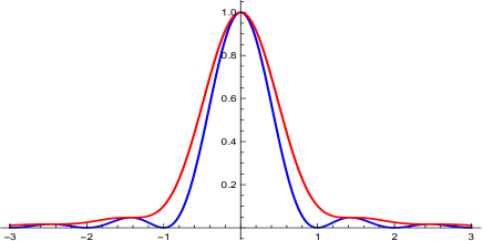
Figure 1. The Fejér kernel $K(x)$ defined in (1.1) and its lid $f(x)$.

1.3. The one-delta problem with derivatives

The function in (1.6) appears in a classical inequality for entire functions. Duffin and Schaeffer [9, p. 239] proved that if a real entire function $g:\mathbb{C}\to\mathbb{C}$ of exponential type at most $\pi$ is such that $|g(x)|\leq 1$ for all $x\in\mathbb{R}$, then

$$|g(x)|^{2}+\dfrac{|g^{\prime}(x)|^{2}}{\pi^{2}}\leq 1,\,\,\,\,\,\,\mbox{for all}\,\,x\in\mathbb{R}.$$

Inspired by this inequality, we prove that specific sums of the $L^{2}-$norms of a function $g\in PW^{2}$, normalized by $g(0)=1$, and its consecutive derivatives, are bounded from below. Our result may be considered a variation of the one-delta problem where one wishes to minimize sums of $L^{2}-$norms of an entire function and of its derivatives, and reads as follows:

Theorem 2.

Let $N$ be a nonnegative integer and the real polynomial

$$\mathcal{P}(x)=\displaystyle\sum_{n=0}^{N}a_{n}x^{n}$$

be positive for every $x\in[0,1]$. Then the inequality

$$\left(\int_{0}^{1}\dfrac{1}{\mathcal{P}(t^{2})}\text{\rm d}t\right)^{-1}\leq\int_{-\infty}^{\infty}\displaystyle\sum_{n=0}^{N}\dfrac{a_{n}}{\pi^{2n}}\big{|}g^{(n)}(x)\big{|}^{2}\,\text{\rm d}x$$ (1.7)

holds for every $g\in PW^{2}$ which obeys the normalization $g(0)=1$. Moreover, equality in (1.7) is attained if and only if

$$g(z)=\left(\int_{0}^{1}\dfrac{1}{\mathcal{P}(t^{2})}\text{\rm d}t\right)^{-1}\int_{0}^{1}\dfrac{\cos{(\pi zt)}}{\mathcal{P}(t^{2})}\,\text{\rm d}t.$$ (1.8)

Note that when $N=0$ and $a_{0}=1$, we recover the inequality (1.3), which once again shows that the latter is a natural result in the spirit of the one-delta problem. Moreover, choosing the polynomial $\mathcal{P}(x)=1+a\pi^{2}x$, we obtain the following corollary.

Corollary 3.

Fix $a>0$. Then the inequality

$$\dfrac{\pi\sqrt{a}}{\arctan(\pi\sqrt{a})}\leq\int_{-\infty}^{\infty}\left(|g(x)|^{2}+a\left|g^{\prime}(x)\right|^{2}\right)\,\text{\rm d}x,$$ (1.9)

holds for every $g\in PW^{2}$ with $g(0)=1$ and the unique extremal function for which (1.9) reduces to an equality is

$$g(z)=\dfrac{\pi\sqrt{a}}{\arctan(\pi\sqrt{a})}\int_{0}^{1}\dfrac{\cos(\pi zt)}{1+a\pi^{2}t^{2}}\,\text{\rm d}t.$$

Observe that for $a=1/\pi^{2}$ (1.9) reduces to the following estimate:

$$\int_{-\infty}^{\infty}\left(|g(x)|^{2}+\frac{\left|g^{\prime}(x)\right|^{2}}{\pi^{2}}\right)\,\!\text{\rm d}x\geq\frac{4}{\pi},\ \ \ g\in PW^{2},\ \ g(0)=1.$$

Different choices of the polynomial $\mathcal{P}(x)$ allow us to obtain other interesting inequalities.

Corollary 4.

Fix $0<a<{1}/{\pi^{2}}$. Then

$$a\int_{-\infty}^{\infty}\big{|}g^{\prime}(x)\big{|}^{2}\text{\rm d}x+\bigg{(}\dfrac{1}{2\pi\sqrt{a}}\,\log\bigg{(}\dfrac{1+\sqrt{a}\pi}{1-\sqrt{a}\pi}\bigg{)}\bigg{)}^{-1}\leq\int_{-\infty}^{\infty}|g(x)|^{2}\,\text{\rm d}x.$$ (1.10)

for every $g\in PW^{2}$ which obeys $g(0)=1$.

In particular, letting $a\to{1}/{\pi^{2}}$ in (1.10) we obtain

$$\int_{-\infty}^{\infty}\big{|}g^{\prime}(x)\big{|}^{2}\,\text{\rm d}x\leq\pi^{2}\int_{-\infty}^{\infty}|g(x)|^{2}\,\text{\rm d}x,\ \ g\in PW^{2},\ \ g(0)=1,$$

which is exactly the $L^{2}-$version of the classical Bernstein inequality that holds for every $L^{p}(\mathbb{R})$, $p\geq 1$ (see [2, Theorem 11.3.3]).

Observe that the Bernstein inequality follows from Theorem 2 if we set $\mathcal{P}(t)=1+\varepsilon-t$ and let $\varepsilon\to 0$. Applying the same reasoning with $\mathcal{P}(t)=(1+\varepsilon-t)^{N}$, we obtain:

Corollary 5.

Let $N$ be a nonnegative integer. Then the inequality

$$\sum_{k=0}^{N}\,\frac{(-1)^{k}}{\sigma^{2k}}\,{N\choose k}\int_{-\infty}^{\infty}\big{|}f^{(k)}(x)\big{|}^{2}\,\text{\rm d}x\geq 0$$

holds for every function of exponential type at most $\sigma$ such that $f\in L^{2}(\mathbb{R})$. In particular, for $N=2$,

$$\int_{-\infty}^{\infty}\big{|}f^{\prime}(x)\big{|}^{2}\,\text{\rm d}x\leq\frac{1}{2}\left(\sigma^{2}\int_{-\infty}^{\infty}\big{|}f(x)\big{|}^{2}\,\text{\rm d}x+\frac{1}{\sigma^{2}}\int_{-\infty}^{\infty}\big{|}f^{\prime\prime}(x)\big{|}^{2}\,\text{\rm d}x\right).$$

The latter is a curious result that resembles some classical ones, due to Landau and Hardy and Littlewood. In 1913, Landau [21] proved that if $f$ is a real function, $f\in C^{2}(\mathbb{R})$, and the inequalities $\|f\|_{\infty}\leq 1$ and $\|f^{\prime\prime}\|_{\infty}\leq 1$ for the uniform norms of $f$ and $f^{\prime\prime}$ on the real line hold, so does $\|f^{\prime}\|_{\infty}\leq\sqrt{2}$.

Hardy and Littlewood [15, Theorem 6] proved that, if $y$ and $y^{\prime\prime}$ are in $L^{2}[0,\infty)$, then

$$\left(\int_{0}^{\infty}[y^{\prime}(x)]^{2}\,\text{\rm d}x\right)^{2}\leq 4\int_{0}^{\infty}[y(x)]^{2}\,\text{\rm d}x\int_{0}^{\infty}[y^{\prime\prime}(x)]^{2}\,\text{\rm d}x.$$

Moreover, the constant $4$ is the best possible. The equality is attained if and only if $y(x)=c\,Y(ax)$, where $c$ and $a$ are real constants and

$$Y(x)=e^{-x/2}\sin\left(\frac{\sqrt{3}}{2}\,x-\frac{\pi}{3}\right).$$

Theorem 7 in [15] states that, under the same requirements, the inequality

$$\int_{0}^{\infty}(y^{2}(x)+[y^{\prime\prime}(x)]^{2}-[y^{\prime}(x)]^{2})\,\text{\rm d}x\geq 0$$

holds with equality as before, but with $a=1$.

2. Proof of Theorem 1: Qualitative aspects

For $f\in L^{1}(\mathbb{R})$, we normalize the Fourier transform $\widehat{f}$ of $f$ as

$$\widehat{f}(\xi)=\int_{-\infty}^{\infty}f(x)e^{-2\pi ix\xi}\,\text{\rm d}x.$$

2.1. Proof of a)

Replacing $f(x)$ by $(f(x)+f(-x))/2$, we see that we may restrict our search for the infimum (1.4) to the even functions in $\mathcal{F}_{1}$. Consider an extremizing sequence $\{f_{n}\}_{n\geq 1}\subset\mathcal{F}_{1}$ such that $f_{n}$ is even, $f_{n}(0)=\|f_{n}\|_{\infty}=1$, and $\|f_{n}\|_{1}\to\mathcal{A}_{1}$. It follows from [22, Theorem 3.3.6], by passing to a subsequence if necessary, that there is $F:\mathbb{C}\to\mathbb{C}$ of exponential type at most $2\pi$ such that $F\in L^{1}(\mathbb{R})$ and

$$f_{n}(x)\to F(x)\ \ \ \mathrm{as}\ \ n\to\infty$$

uniformly on any compact set of $\mathbb{C}$. Therefore, $F$ is even, $F\in\mathcal{F}_{1}$ and $F(0)=1$. Fatou’s lemma implies that $\|F\|_{1}\leq\mathcal{A}_{1}$, and by the definition of $\mathcal{A}_{1}$ as an infimum we conclude that $F$ is an extremizer for (1.4).

2.2. Proof of b)

Let $F$ be an even extremizer with $F(0)=1$. Clearly, it has no real zeros. Indeed, since $F$ is real, nonnegative and decreasing on the positive real axis, if it vanishes at $x_{0}>0$, it does for all $x>x_{0}$ which is impossible because $F$ is entire and $F(0)=1$. Since $F$ is even, also it does not vanish at a negative $x_{0}$. Therefore, all the zeros of $F$ satisfy $|{\rm Im}\,{z}|>0$. Now, assume that $F$ has a zero at $z=ib$, for $b\in\mathbb{R}$. Since $F$ is real-valued, it also has $z=-ib$ as a zero. Consider the entire function

$$G(z)=\dfrac{b^{2}F(z)}{z^{2}+b^{2}}.$$

Note that $G(0)=1$ and $G\in\mathcal{F}_{1}$. Since

$$\int_{-\infty}^{\infty}G(x)\,\text{\rm d}x<\int_{-\infty}^{\infty}F(x)\,\text{\rm d}x$$

we get a contradiction. Therefore, all the zeros of $F$ satisfy $|{\rm Re}\,{z}|>0$. Now, assume that $z=a+ib$ is a zero of $F$ with $|b|\geq|a|>0$. Since $F$ is real-valued and even, we have that $z=a-ib$, $z=-a+ib$, and $z=-a-ib$ are also zeros. Note that all these zeros are different. Then, the entire function

$$H(z)=\dfrac{(a^{2}+b^{2})^{2}F(z)}{\left((z-a)^{2}+b^{2}\right)\left((z+a)^{2}+b^{2}\right)}$$

is in $\mathcal{F}_{1}$, and using that $|b|\geq|a|$, it is easy to see that

$$\int_{-\infty}^{\infty}H(x)\,\text{\rm d}x<\int_{-\infty}^{\infty}F(x)\,\text{\rm d}x$$

which gives a contradiction. We conclude that $|b|<|a|$.

3. Proof of Theorem 1: quantitative aspects

3.1. Representation lemma

The following lemma gives a representation for any even function in $\mathcal{F}_{1}$.

Lemma 6.

If $f\in\mathcal{F}_{1}$ is even, then it can be represented in $\mathbb{R}$ in the form

$$f(x)=\int_{-\infty}^{x}-t\,|h(t)|^{2}\,\text{\rm d}t,$$ (3.1)

where $h:\mathbb{C}\to\mathbb{C}$ is an entire function of exponential type at most $\pi$ such that $|h(x)|=|h(-x)|$ for all $x\in\mathbb{R}$, and $xh\in L^{2}(\mathbb{R})$. Conversely, if $f$ is a function of the form (3.1), then it has an analytic extension to $\mathbb{C}$ which is an even function in $\mathcal{F}_{1}$.

Proof.

Let $f\in\mathcal{F}_{1}$ be even. Integration by parts yields

$$\int_{0}^{x}f(t)\,\text{\rm d}t=xf(x)+\int_{0}^{x}t\,|f^{\prime}(t)|\,\text{\rm d}t.$$ (3.2)

Since the integrals on both sides of (3.2) are increasing functions of $x$, and $f\in L^{1}(\mathbb{R})$, when $x\to+\infty$ we can conclude that $\displaystyle\lim_{x\to\infty}xf(x)$ exists (similarly $\displaystyle\lim_{x\to-\infty}xf(x)$ exists). The fact that $f\in L^{1}(\mathbb{R})$ forces these limits to be zero and one can also conclude that $x\,f^{\prime}(x)\in L^{1}(\mathbb{R})$. By the Plancherel-Pólya theorem, $f^{\prime}(z)$ has exponential type $2\pi$ and so does $-zf^{\prime}(z)$. From the Krein decomposition theorem [1, p. 154], it follows that $-zf^{\prime}(z)=g(z)g^{*}(z)$ for some $g\in PW^{2}$. Moreover, since $f$ attains its maximum at $x=0$, then $f^{\prime}(0)=0$. Defining $h(z)=g(z)/z$, we rewrite the latter in the form

$$-zf^{\prime}(z)=z^{2}h(z)h^{*}(z),$$ (3.3)

where $h$ is an entire function of exponential type at most $\pi$ and $xh\in L^{2}(\mathbb{R})$. Since $f^{\prime}$ is odd, then $|h(x)|=|h(-x)|$ for $x\in\mathbb{R}$. Finally, integrating (3.3) appropriately, we arrive at (3.1). Conversely, assume the representation (3.1). Note that $f$ has an analytic extension on $\mathbb{C}$ (also denoted by $f$) of the form

$$f(z)=\int_{-\infty}^{0}-t|h(t)|^{2}\,\text{\rm d}t+\int_{[0,z]}-s\,h(s)h^{*}(s)\,\text{\rm d}s,$$

where $[0,z]$ denotes the straight segment connecting $0$ and $z$. Since $h$ is an entire function of exponential type at most $\pi$, $f$ is an entire function of exponential type at most $2\pi$. From (3.1) it follows that $\displaystyle\lim_{x\to-\infty}f(x)=0$, and using the fact that $|h(x)|=|h(-x)|$, we conclude that $f$ is also even and $\displaystyle\lim_{x\to\infty}f(x)=0$. On the other hand, differentiating (3.1) we derive

$$f^{\prime}(x)=-x\,|h(x)|^{2}\ \ \ \mathrm{for}\ \ x\in\mathbb{R},$$ (3.4)

which implies that $f$ is radially decreasing and $f(x)\geq 0$. Moreover, (3.4) and $xh\in L^{1}(\mathbb{R})$ imply $\displaystyle\lim_{x\to\pm\infty}xf(x)=0$. Integration by parts shows that

$$\int_{-\infty}^{\infty}f(x)\,\text{\rm d}x=\int_{-\infty}^{\infty}x^{2}|h(x)|^{2}\,\text{\rm d}x,$$

which yields $f\in L^{1}(\mathbb{R})$. ∎

From Lemma 6, we can reformulate the monotone-delta problem as the one to determine

$$\mathcal{A}_{1}=\inf_{\begin{subarray}{c}h\in\mathcal{F}_{2}\\ h\not\equiv 0\end{subarray}}\dfrac{2\displaystyle\int_{-\infty}^{\infty}|x|^{2}|h(x)|^{2}\,\text{\rm d}x}{\displaystyle\int_{-\infty}^{\infty}|x||h(x)|^{2}\,\text{\rm d}x},$$ (3.5)

where the family $\mathcal{F}_{2}$ consists of those entire functions $h:\mathbb{C}\to\mathbb{C}$ of exponential type at most $\pi$ such that $xh\in L^{2}(\mathbb{R})$ and $|h(x)|=|h(-x)|$.

3.2. An $L^{2}-$computational approach

A natural approach for constructing functions in $\mathcal{F}_{2}$ (and therefore in $\mathcal{F}_{1}$), and computationally solving (3.5), starts by finding an orthonormal system for the space $L^{2}(\mathbb{R},x^{2}\text{\rm d}x)$. Note that $\mathcal{F}_{2}$ is a Hilbert space with the inner product

$$\langle f,g\rangle_{\mathcal{F}_{2}}=\langle xf,xg\rangle_{L^{2}(\mathbb{R})},$$

and norm

$$\|f\|_{\mathcal{F}_{2}}=\left(\int_{-\infty}^{\infty}|x|^{2}|f(x)|^{2}\,\text{\rm d}x\right)^{\!\frac{1}{2}}.$$ (3.6)

For positive integers $k$, we define the even functions

$$h_{k}(x)=\frac{4\sqrt{2}}{\pi}\cdot\frac{\cos\pi x}{(2k-1)^{2}-4x^{2}},$$ (3.7)

and note that $h_{k}\in\mathcal{F}_{2}$ for all positive integers $k$. Gorbachev [11] previously considered this family of functions to obtain fine numerical estimates for other Fourier extremal problems, and it has also been used in [8] for similar purposes in related extremal problems introduced by Carneiro, Milinovich, and Soundararajan [4]. Regarding this system, we can say the following:

Proposition 7.

The family $(h_{k})_{\begin{subarray}{c}k\geq 1\end{subarray}}$ is a complete orthonormal system in the closed subspace $\{h\in\mathcal{F}_{2}:\ h\text{ is even.}\}.$

Proof.

Note that, if $h\in\mathcal{F}_{2}$ is even, then $xh\in L^{2}(\mathbb{R})$ is odd. Furthermore, we have that

$$\widehat{(xh_{k})}(t)=i(-1)^{k}\sqrt{2}\sin(\pi(2k-1)t)\chi_{I}(t)=:s_{k}(t),$$ (3.8)

where $I=[-1/2,1/2]$ and $\chi_{I}$ denotes the characteristic function of the interval $I$. To see this, since $s_{k}\in L^{1}(\mathbb{R})\cap L^{2}(\mathbb{R})$, we may compute $\widehat{s}_{k}$ in a straightforward manner to verify that $\widehat{s}_{k}(x)=-xh_{k}(x)$, and then we conclude (3.8) by Fourier inversion in $L^{2}(\mathbb{R})$. Now consider the operator

$$T:\mathcal{F}_{2}\to L^{2}(I)$$

defined by $Th(t):=\widehat{(xh)}(t)e^{\pi it}$. By Plancherel’s theorem and the Paley-Wiener theorem, $T$ is a linear isometry, that is, $\langle f,g\rangle_{\mathcal{F}_{2}}=\langle Tf,Tg\rangle_{L^{2}(I)}$. Therefore, for positive integers $k$ and $j$, we find that

$$\langle h_{k},h_{j}\rangle_{\mathcal{F}_{2}}=\langle s_{k},s_{j}\rangle_{L^{2}(I)}=\delta_{kj},$$

where $\delta_{kj}=1$ if $k=j$, and $0$ otherwise. Here, to compute the inner product over $L^{2}(I)$, we may apply the identity $2\sin(\pi(2k-1)t)\sin(\pi(2j-1)t)=\cos(2\pi(k-j)t)-\cos(2\pi(k+j-1)t)$. This shows that $h_{k}$ is orthonormal.

We now show that it is complete. Let $h\in\mathcal{F}_{2}$ be even, such that $\langle h,h_{k}\rangle_{\mathcal{F}_{2}}=0$ for all positive integers $k$. We must show that $h\equiv 0$. First, denote $H(t)=\widehat{(xh)}(t)$, and note that, by Plancherel’s theorem and (3.8), the condition $\langle h,h_{k}\rangle_{\mathcal{F}_{2}}=0$ implies that

$$\int_{I}H(t)\sin(\pi(2j-1)t)\,\text{\rm d}t=0$$ (3.9)

for all positive integers $j$. Actually, since $\sin(-x)=-\sin x$, (3.9) holds for all integers $j$.

Now, since $T$ is an isometry into $L^{2}(I)$, by the theory of Fourier series on $L^{2}(I)$, it is enough to show that $\langle Th,e_{j}\rangle_{L^{2}(I)}=0$ for all integers $j$, where $e_{j}(t)=e^{2\pi ijt}$. In fact, for an integer $j$, we have

$$\begin{split}\langle Th,e_{j}\rangle_{L^{2}(I)}&=\int_{I}H(t)e^{\pi it}e^{-2\pi itj}\,\text{\rm d}t\\ &=\int_{I}H(t)\cos(\pi(2j-1)t)\,\text{\rm d}t-i\int_{I}H(t)\sin(\pi(2j-1)t)\,\text{\rm d}t.\end{split}$$

The first integral in the last line is 0 since $H$ is odd, and the second integral is 0 by (3.9). Therefore, $\langle Th,e_{j}\rangle_{L^{2}(I)}=0$ for all integers $j$, and then $Th\equiv 0$ and $h\equiv 0$, as desired. ∎

More general orthogonality results can also be obtained from the theory of de Branges spaces; see [5, Section 2.2] and the references therein. See also [13, Theorem 4.2] for a similar general orthogonality result.

3.3. Proof of c): Generating bounds

Once we have a complete orthonormal system, we proceed to obtain numerical examples as follows. For a positive integer $d$, let $\mathcal{F}_{2,d}=\,$span $\{h_{k}:1\leq k\leq d\}\subset\mathcal{F}_{2}$. Let $Q\in\mathbb{R}^{d\times d}$ be the matrix defined by

$$Q_{kj}=\int_{0}^{\infty}x\,h_{k}(x)h_{j}(x)\,\text{\rm d}x.$$ (3.10)

Then, since $h_{k}$ are orthonormal, one can see that the reciprocal of the infimum in (3.5), when taken over the space $\mathcal{F}_{2,d}$, satisfies

$$|\lambda_{d}|=\max_{\begin{subarray}{c}h\in\mathcal{F}_{2,d}\\ h\not\equiv 0\end{subarray}}\dfrac{\displaystyle\int_{0}^{\infty}x\,|h(x)|^{2}\,\text{\rm d}x}{\displaystyle\int_{-\infty}^{\infty}|x|^{2}|h(x)|^{2}\,\text{\rm d}x},$$

where $\lambda_{d}$ is the largest eigenvalue (in absolute value) of $Q$, and the maximum is attained when

$$h=\mathbf{a}\cdot(h_{1},h_{2},\ldots,h_{d}),$$ (3.11)

for $\mathbf{a}\in\mathbb{R}^{d}$ an eigenvector of $Q$ associated to $\lambda_{d}$. In particular, we have that $\mathcal{A}_{1}\leq|\lambda_{d}|^{-1}$. Moreover, we now proceed to prove that as $d\to\infty$, we have $|\lambda_{d}|^{-1}\to\mathcal{A}_{1}$. Furthermore, we are able to explicitly estimate the speed of convergence, yielding lower bounds that also converge to $\mathcal{A}_{1}$ (see Theorem 8 below). With that goal in mind, we proceed to study the coefficients $Q_{kj}$ defined in (3.10). Our first observation is that they can be made more explicit. When $k>j$, we expand in partial fractions and use the trigonometric identity $2\cos^{2}(x)=1+\cos(2x)$ to see that

$$(k-j)(k+j-1)Q_{kj}=\int_{0}^{\infty}\frac{32(k-j)(k+j-1)x\cos^{2}(\pi x)}{\pi^{2}(4x^{2}-(2k-1)^{2})(4x^{2}-(2j-1)^{2})}\text{\rm d}x$$

$$=\int_{0}^{\infty}\frac{1+\cos(2\pi x)}{\pi^{2}}\left(\frac{1}{2x-(2k-1)}+\frac{1}{2x+(2k-1)}-\frac{1}{2x-(2j-1)}-\frac{1}{2x+(2j-1)}\right)\text{\rm d}x.$$

By carefully splitting the integral, changing variables by translations and dilations, and regrouping all the pieces, one obtains

$$Q_{kj}=\dfrac{-1}{\pi^{2}\,(k-j)\,(k+j-1)}\displaystyle\int_{2j-1}^{2k-1}\frac{1-\cos(\pi x)}{x}\,\text{\rm d}x.$$

When $k=j$, a similar argument leads to the expression

$$Q_{kk} =\dfrac{2}{\pi^{2}(2k-1)}\int_{0}^{2k-1}\frac{1-\cos(\pi x)}{x^{2}}\,\text{\rm d}x=\dfrac{-4+2(2k-1)\pi\,\text{Si}(\pi(2k-1))}{\pi^{2}\,(2k-1)^{2}},$$

where $\mathrm{Si}(x)=\int_{0}^{x}\sin(t)/t\,\text{\rm d}t$ is the standard sine integral function. These expressions readily imply that

$$|Q_{kj}|\lesssim\frac{1}{d\,(k-j)},\,\,\,\,\,\mbox{and}\,\,\,\,\,|Q_{kk}|\lesssim\frac{1}{(2k-1)},\,\,\,\,\,\mathrm{when}\,\,d\leq j<k.$$

These inequalities, with effective constants, lead to bounds that can be used to explicitly estimate the speed of convergence of $|\lambda_{d}|^{-1}$ to $\mathcal{A}_{1}$. By taking a particular value of $d$, we obtain the bounds stated in Theorem 1. Before we state our general bounds, we briefly remark that, from the aforementioned work [5] (see Theorem 2 therein), we may restrict the search for the infimum in (1.5) to even functions $h\in\mathcal{F}_{2}$.

Theorem 8.

Let $h\in\mathcal{F}_{2}$ be even and not identically 0. Define $h_{k}$ as in (3.7), and for a positive integer $d$, let $\lambda_{d}$ be the maximum eigenvalue (in absolute value) of the matrix $Q$ defined in (3.10). Then, for $d\geq 1000$,

$$\int_{-\infty}^{\infty}|x|\,|h(x)|^{2}\,\text{\rm d}x<2\left({\displaystyle\int_{-\infty}^{\infty}|x|^{2}|h(x)|^{2}\,\text{\rm d}x}\right)\left(|\lambda_{d}|+\frac{\sqrt{\log d}}{d}+\frac{1}{d}\right).$$

In particular, for any $d\geq 1000$, we have

$$\left(|\lambda_{d}|+\frac{\sqrt{\log d}}{d}+\frac{1}{d}\right)^{-1}<\mathcal{A}_{1}\leq|\lambda_{d}|^{-1}.$$

When $d=3010$, one obtains

$$1.2750<\mathcal{A}_{1}<1.27714.$$

Proof.

Write $h=\sum_{k=1}^{\infty}a_{k}h_{k}$, with $a_{k}\in\mathbb{C}$. Denote $\mathbf{a}=(a_{k})_{k\geq 1}$ and $\|\mathbf{a}\|_{2}:=\sqrt{\sum_{k\geq 1}|a_{k}|^{2}}$, so that $\|h\|_{\mathcal{F}_{2}}=\|\mathbf{a}\|_{2}$ (see (3.6)). Now, consider the functional $J:\mathcal{F}_{2}\backslash\{0\}\to\mathbb{R}$ given by

$$J(h):=\frac{\displaystyle\int_{0}^{\infty}x\,|h(x)|^{2}\,\text{\rm d}x}{\displaystyle\int_{-\infty}^{\infty}|x|^{2}|h(x)|^{2}\,\text{\rm d}x}.$$

First note that $J$ is continuous on $\{h\in\mathcal{F}_{2}:\,h\not\equiv 0\}$. Indeed, from the classical one-delta problem, we have the trivial lower bound $\mathcal{A}_{1}\geq 1.$ For $f_{1},$ $f_{2}\in\mathcal{F}_{2}$, the triangle inequality yields

$$\left|\sqrt{\int_{0}^{\infty}|x|\,|f_{1}(x)|^{2}\,\text{\rm d}x}-\sqrt{\int_{0}^{\infty}|x|\,|f_{2}(x)|^{2}\,\text{\rm d}x}\right|\leq\sqrt{\int_{0}^{\infty}|x|\,|f_{1}(x)-f_{2}(x)|^{2}\,\text{\rm d}x}\leq\|f_{1}-f_{2}\|_{\mathcal{F}_{2}},$$

which implies the desired continuity. Here, we used that $\mathcal{A}_{1}\leq 1$ in the last inequality. Now, fix $d\geq 1000$, and for a parameter $M\geq d$, consider $H_{M}=\sum_{k=1}^{M}a_{k}h_{k}$. One has

$$J(H_{M})\cdot\left(|a_{1}|^{2}+|a_{2}|^{2}+\ldots+|a_{M}|^{2}\right) =\sum_{k,j=1}^{d}a_{k}\overline{a_{j}}\,Q_{kj}+2\,{\rm Re}\,\sum_{\begin{subarray}{c}d<k\leq M\\ 1\leq j\leq d\end{subarray}}a_{k}\overline{a_{j}}\,Q_{kj}+\sum_{k,j=d+1}^{M}a_{k}\overline{a_{j}}\,Q_{kj}$$

$$=J(H_{d})\cdot\left(|a_{1}|^{2}+|a_{2}|^{2}+\ldots+|a_{d}|^{2}\right)+J_{1}+J_{2}$$ (3.12)

Here, $Q_{kj}$ is defined as in equation (3.10). By definition of $\lambda_{d}$, we have $|J(H_{d})|\leq|\lambda_{d}|$. We now estimate $|J_{1}|$ and $|J_{2}|$. One can verify that $Q_{kk}>0$ and that $Q_{kj}<0$ for $k\neq j$. To obtain upper bounds for $|Q_{kj}|$, note that, since the local maxima of Si$(x)$ form a decreasing sequence, we have $0<\text{Si}(\pi(2k-1))\leq\text{Si}(2001\pi)$ for all $k>1000$. Additionally, since $|\cos(\pi x)|\leq 1$, we have that, for $1\leq j<k$:

$$0<\int_{2j-1}^{2k-1}\frac{1-\cos(\pi x)}{x}\,\text{\rm d}x\leq\int_{2j-1}^{2k-1}\frac{2}{x}\,\text{\rm d}x=2\log\left(1+\frac{2(k-j)}{2j-1}\right).$$

This yields the inequalities

$$|Q_{kj}|\leq\frac{2\log\left(1+\tfrac{2(k-j)}{2j-1}\right)}{\pi^{2}\,(k-j)\,(k+j-1)},\,\,\,\,\,\,\,\,\,\,\,\mbox{and}\,\,\,\,\,\,\,\,\,\,\,\,|Q_{kk}|\leq\frac{2\,\text{Si}(2001\pi)}{\pi(2k-1)}$$

for $1\leq j<k$, and for $k>1000$ respectively. To estimate $|J_{1}|$ we use the triangle inequality, extend the sum over $k$ to infinity and apply the Cauchy-Schwarz inequality in both variables, which yields

$$|J_{1}| \leq\frac{4}{\pi^{2}}\sum_{\begin{subarray}{c}d<k\\ 1\leq j\leq d\end{subarray}}\,\frac{\log\left(1+\tfrac{2(k-j)}{2j-1}\right)}{(k-j)(k+j-1)}|a_{k}a_{j}|$$

$$\leq\frac{4}{\pi^{2}}\left(\sum_{\begin{subarray}{c}d<k\\ 1\leq j\leq d\end{subarray}}\,\frac{\log^{2}\left(1+\tfrac{2(k-j)}{2j-1}\right)}{(k-j)^{2}(k+j-1)^{2}}\right)^{\!\!\frac{1}{2}}\left(\sum_{k,j=1}^{\infty}|a_{k}|^{2}|a_{j}|^{2}\right)^{\!\!\frac{1}{2}}$$

$$\leq\frac{4}{\pi^{2}}\left(\sum_{j=1}^{d}\frac{1}{(j+d)^{2}}\,\sum_{k=d+1}^{\infty}\frac{\log^{2}\left(1+\tfrac{2(k-j)}{2j-1}\right)}{(k-j)^{2}}\right)^{\!\!\frac{1}{2}}\|\mathbf{a}\|_{2}^{2}.$$ (3.13)

Since $k-j\geq 1$, by applying estimates (5.5) and (5.6) with $n=d$ and $t={2}/{(2j-1)}$ in (3.3), we obtain

$$|J_{1}| \leq\frac{4}{\pi^{2}}\left(\sum_{j=1}^{d}\frac{4}{(j+d)^{2}(2j-1)^{2}}+\frac{\pi^{2}}{3}\sum_{j=1}^{d}\frac{2}{(j+d)^{2}(2j-1)}\right)^{\!\!\frac{1}{2}}\|\mathbf{a}\|_{2}^{2}$$

$$\leq\frac{4}{\pi^{2}d}\left(\sum_{j=1}^{\infty}\frac{4}{(2j-1)^{2}}+\frac{\pi^{2}}{3}\sum_{j=1}^{d}\frac{2}{(2j-1)}\right)^{\!\!\frac{1}{2}}\|\mathbf{a}\|_{2}^{2}$$

$$\leq\frac{4}{\pi^{2}d}\left(\frac{\pi^{2}}{2}+\frac{\pi^{2}}{2}\log d\right)^{\!\!\frac{1}{2}}\|\mathbf{a}\|_{2}^{2}.$$

In particular, when $d\geq 1000$,

$$|J_{1}|\leq\frac{2\sqrt{2}}{\pi}\left(1+\frac{1}{\log 1000}\right)^{\!\!\frac{1}{2}}\frac{\sqrt{\log d}}{d}\|\mathbf{a}\|_{2}^{2}<\frac{\sqrt{\log d}}{d}\|\mathbf{a}\|^{2}.$$ (3.14)

To estimate $|J_{2}|$, we first separate the diagonal term $k=j$. On the other terms, we use the fact that $x\mapsto{\log(1+ax)}/{x}$ is decreasing when $x\in[0,\infty)$ for any $a>0$, and the Cauchy-Schwarz inequality, to obtain

$$|J_{2}| \leq\frac{2\,\text{Si}(2001\pi)}{\pi(2d+1)}\cdot\sum_{k>d}|a_{k}|^{2}+\frac{4}{\pi^{2}}\sum_{\begin{subarray}{c}k>j\\ k,\,j>d\end{subarray}}|a_{k}||a_{j}|\frac{\log\left(1+\tfrac{2}{2j-1}\right)}{k+j-1}$$

$$\leq\frac{\,\text{Si}(2001\pi)}{\pi\,d}\|\mathbf{a}\|_{2}^{2}+\frac{8}{\pi^{2}}\left(\sum_{\begin{subarray}{c}k>j\\ k,\,j>d\end{subarray}}\frac{1}{(k+j-1)^{2}(2j-1)^{2}}\right)^{\!\!\frac{1}{2}}\|\mathbf{a}\|_{2}^{2}$$

By applying (5.4) with $n=2j$ followed by (5.7) with $n=d+1$, one arrives at

$$|J_{2}|\leq\frac{\,\text{Si}(2001\pi)}{\pi\,d}\|\mathbf{a}\|_{2}^{2}+\frac{8}{\pi^{2}}\left(1+\frac{1}{1000}\right)^{\!\!\frac{1}{2}}\left(\sum_{j=d+1}^{\infty}\frac{1}{2j(2j-1)^{2}}\right)^{\!\!\frac{1}{2}}\|\mathbf{a}\|_{2}^{2}<\frac{1}{d}\|\mathbf{a}\|^{2}.$$ (3.15)

Since (3.14) and (3.15) do not depend on $M$, applying these estimates on (3.3), sending $M\to\infty$, and using the continuity of $J$ concludes the proof. Finally, to obtain numerical bounds, we calculate the eigensystems numerically for $d\leq 3010$, and find that $0.783002554179<\lambda_{3010}<0.783002554181$. We thereby obtain the numerical bounds in Theorem 8, and we highlight here our best, rigorous upper bound:

$$\mathcal{A}_{1}<1.277135042105.$$

∎

4. Some functions in $\mathcal{F}_{1}$

4.1. The lid function

In this subsection, we apply Sonin’s method to construct a nice sequence of functions in $\mathcal{F}_{1}$. For any positive real numbers $B$ and $C$, consider the differential equation

$$y^{\prime\prime}+\dfrac{B}{x}\,y^{\prime}+Cy=0.$$ (4.1)

Let $y=g$, $g:\mathbb{R}\to\mathbb{R}$ be a solution of the equation (4.1). The lid of $g^{2}$ is the function defined by

$$f(x)=(g(x))^{2}+\dfrac{(g^{\prime}(x))^{2}}{C}.$$ (4.2)

Note that $f(x)\geq 0$ for all $x\in\mathbb{R}$, and

$$f^{\prime}(x)=-\dfrac{2B(g^{\prime}(x))^{2}}{x\,C}.$$

This implies that $f$ is radially decreasing. Moreover, if we suppose that the solution $g$ has an analytic extension on $\mathbb{C}$ of exponential type at most $\pi$, and $g\in L^{2}(\mathbb{R})$, we conclude that $f\in\mathcal{F}_{1}$.

Let us show some examples of lids. For $\alpha>0$, consider the Bessel function of the first kind of order $\alpha$, which is defined by

$$J_{\alpha}(z)=\displaystyle\sum_{\nu=0}^{\infty}\dfrac{(-1)^{\nu}(z/2)^{\alpha+2\nu}}{\nu!\,\Gamma(\nu+\alpha+1)}.$$

Let us remark some properties of the Bessel functions mentioned in [25, Section 1.71]. It is known (see [25, Equation 1.71.3]) that $J_{\alpha}$ satisfies the differential equation

$$y^{\prime\prime}+x^{-1}y^{\prime}+(1-\alpha^{2}x^{-2})y=0.$$ (4.3)

Now, define the function

$$g_{\alpha}(z)=\dfrac{J_{\alpha}(\pi z)}{(\pi z)^{\alpha}}.$$

A straightforward change of variables in (4.3) shows that $g_{\alpha}$ satisfies the differential equation

$$y^{\prime\prime}+\dfrac{2\alpha+1}{x}\,y^{\prime}+\pi^{2}y=0.$$

The function $g_{\alpha}$ is an even entire function of exponential type $\pi$. Moreover, using the decay of $J_{\alpha}$ (see [25, Equations 1.71.10 and 1.71.11] we see that $g_{\alpha}\in L^{2}(\mathbb{R})$. Therefore, inserting $g_{\alpha}$ in (4.2) we actually construct the lid of $g_{\alpha}^{2}$, with $B=2\alpha+1$ and $C=\pi^{2}$. In the particular case $\alpha=1/2$ we known that

$$g_{1/2}(x)=\dfrac{\sin(\pi x)}{\pi x},$$

and therefore

$$f_{1/2}(x)=(g_{1/2}(x))^{2}+\dfrac{(g_{1/2}^{\prime}(x))^{2}}{\pi^{2}}$$

is the lid of $K(x)$. Straightforward calculations show that the Fourier transform of $f_{1/2}$ is

$$\widehat{f_{1/2}}(\xi)=\max\{1-|\xi|,0\}+\dfrac{1}{\pi^{2}}\widehat{(g^{\prime}_{1/2})^{2}}(\xi).$$ (4.4)

Then the Fourier transform - convolution de Margan type law yields

$$\widehat{(g_{1/2}^{\prime})^{2}}(\xi) =(\widehat{g_{1/2}^{\prime}}\ast\widehat{g_{1/2}^{\prime}})(\xi)=\left((2\pi ix\,\widehat{g_{1/2}})\ast(2\pi ix\,\widehat{g_{1/2}})\right)\!(\xi)=-4\pi^{2}\int_{-\infty}^{\infty}x\widehat{g_{1/2}}(x)(\xi-x)\widehat{g_{1/2}}(\xi-x)\,\text{\rm d}x,$$

where we used the fact that $\widehat{g_{1/2}}(x)=\chi_{I}(x)$. This, together with (4.4), implies

$$\widehat{f_{1/2}}\,(\xi)=\left\{\begin{array}[]{ll}\dfrac{2}{3}\,(1-|\xi|)^{2}(|\xi|+2),&\mathrm{if\ }|\xi|\leq 1;\\ 0,&\mathrm{if\ }|\xi|>1.\end{array}\right.$$

In particular, this example allows us to obtain the bound $\mathcal{A}_{1}\leq 1.333\ldots$. In fact, one can repeat the same argument for the function $f_{\alpha}$, for any $\alpha>0$. The Fourier transform of $f_{\alpha}$ can be computed using [25, Equation 1.71.6]. Finally, we minimize the ratio $\widehat{f_{\alpha}}(0)/f_{\alpha}(0)$ with respect to $\alpha$, and obtain that it is attained for $\alpha_{0}=0.787\ldots$ and $\widehat{f_{\alpha_{0}}}(0)/f_{\alpha_{0}}(0)=1.284\ldots$. Hence $\mathcal{A}_{1}\leq 1.284\ldots$.

4.2. Polynomial examples

As mentioned in the introduction, we now transform the optimization problem (3.5) over $\mathcal{F}_{2}$ in into another unrestricted, smooth optimization problem over $\mathbb{R}^{d+1}$, so that we may construct functions $h$ in a systematic way with standard numerical optimization methods. For this purpose, we make a couple of helpful observations. First, note that if $h\in\mathcal{F}_{2}$ then $h\in L^{1}(\mathbb{R})$. In fact, by the Cauchy-Schwarz inequality, we have

$$\int_{1}^{\infty}|h(x)|\ \text{\rm d}x =\int_{1}^{\infty}|x\,h(x)|\cdot\frac{1}{x}\,\text{\rm d}x\leq\sqrt{\int_{1}^{\infty}x^{2}|h(x)|^{2}\,\text{\rm d}x}\cdot\sqrt{\int_{1}^{\infty}\frac{1}{x^{2}}\,\text{\rm d}x}\,<\infty.$$

Therefore, $\widehat{h}$ is continuous in $\mathbb{R}$, and in particular $\widehat{h}(\pm 1/2)=0$. Denoting $I=[-1/2,1/2]$ we have that $\operatorname{\mathrm{supp}}\widehat{h}\subset I$. Therefore, by the Stone-Weierstrass theorem we may approximate $\widehat{h}$ uniformly by a polynomial times $\chi_{I}$.

With the previous observations in mind, we consider functions of the form

$$\widehat{h}(x)=\left(\frac{1}{4}-x^{2}\right)g(x)\chi_{I}(x),$$ (4.5)

where

$$g(x)=\sum_{i=0}^{d}a_{i}x^{i}\in\mathbb{R}[x]$$

is a polynomial of degree $d$. Note that the factor $\left(\frac{1}{4}-x^{2}\right)$ means that $\widehat{h}\left(\pm 1/2\right)=0.$ Denoting $\mathbf{a}=(a_{0},a_{1},\ldots,a_{d})\in\mathbb{R}^{d+1}$, the infimum in (3.5), restricted to this class, becomes

$$\mathcal{A}_{1,d}:=\min_{\mathbf{a}\in\mathbb{R}^{d+1}\setminus 0}\dfrac{2\mathbf{a}\cdot N\mathbf{a}}{\mathbf{a}\cdot D\mathbf{a}},$$ (4.6)

where $N$, $D\in\mathbb{R}^{(d+1)\times(d+1)}$ are defined by

$$N_{ij}=\int_{-\infty}^{\infty}|x|^{2}f_{i}(x)\overline{f_{j}(x)}\,\text{\rm d}x;\ \ \ D_{ij}=\int_{-\infty}^{\infty}|x|f_{i}(x)\overline{f_{j}(x)}\,\text{\rm d}x;\ \ \ f_{i}(x)=\left[\left(\frac{1}{4}-y^{2}\right)y^{i}\chi_{I}\right]^{\wedge}\!\!\!(-x).$$

For all $d\leq 20$ and $0\leq i\leq d$, it is easy to see by direct computation of $f_{i}$ that $xf_{i}\in L^{2}(\mathbb{R})$, so that $h=\mathbf{a}\cdot(f_{0},\ldots,f_{d})\in\mathcal{F}_{2}$ for all $\mathbf{a}\in\mathbb{R}^{d+1}$. The matrices $N$ and $D$ may be computed explicitly for a given $d$, and this is then a smooth optimization problem over $\mathbb{R}^{d+1}$. Solving it numerically for $d=2$, we find

$$\widehat{h_{0}}(x)=\left(\frac{1}{4}-x^{2}\right)\left(1-\frac{9}{5}x^{2}\right)\chi_{I}(x),$$ (4.7)

which yields

$$h_{0}(x)=\frac{\left(108-25\pi^{2}x^{2}\right)\sin(\pi x)-\pi x\left(11\pi^{2}x^{2}+108\right)\cos(\pi x)}{40\pi^{5}x^{5}}.$$ (4.8)

By direct computation in exact rational arithmetic, this gives

$$\mathcal{A}_{1}\leq\frac{49484}{38745}=1.27717...$$

This gives another proof of an upper bound for $\mathcal{A}_{1}$, which coincides up to four decimal digits with our best bounds. Moreover, using the representation (3.1) we obtain the function in $\mathcal{F}_{1}$

$$\begin{split}f_{0}(x)=&\frac{P(\pi x)+Q(\pi x)\sin(2\pi x)+R(\pi x)\cos(2\pi x)}{738\pi^{8}x^{8}},\end{split}$$ (4.9)

where

$$P(x)= \!\!\!\!242x^{6}+3001x^{4}+4176,$$

$$Q(x)= \!\!\!\!-242x^{5}-576x^{3}-11664x,$$

$$R(x)= \!\!\!\!1463x^{4}+7488x^{2}-5832;$$

see Figure 2.

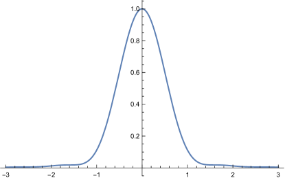
Figure 2. The function $f_{0}(x)$ defined in equation (4.9).

Additionally, we solve (4.6) for all $d\leq 20$ and observe that, as the degree $d$ increases, the sequence $\mathcal{A}_{1,d}$ decreases very slowly, showing only a tiny improvement from $1.27717...$ only in the fifth decimal digit. More precisely, we recover the bound $\mathcal{A}_{1}\leq 1.27713505...$ with those much more detailed calculations performed with large degree $d$ of the polynomials $g$. Below, we will show some tables with the results of these computations (see Table 1), and compare the results with those of our $L^{2}$-approach from Section 3.2. In Figure 4 and Figure 4, we plot the functions $4\widehat{h}_{0}$ and $\frac{600}{91}h_{0}$, respectively, where, since $h_{0}(0)=\frac{91}{600}$ and $\widehat{h}_{0}(0)=\frac{1}{4}$, we renormalized the plots accordingly.

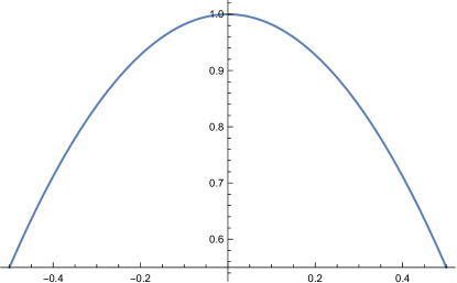
Figure 3. The function $\widehat{h_{0}}(x)/\widehat{h_{0}}(0)$ defined in equation (4.7).

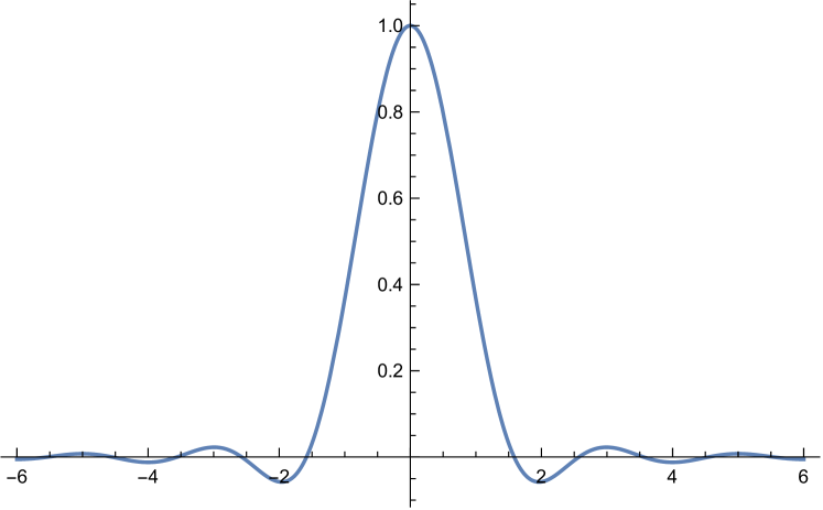
Figure 4. The function $h_{0}(x)/h_{0}(0)$ defined in equation (4.8).

In Table 1, we compare the speed of convergence of the two numerical approaches we have presented. The first approach is described above in the present section , with functions $h$ defined as in (4.5), via polynomials $g$ of some degree $d$. The second approach is the $L^{2}-$approach described in Section 3.2, with functions $h$ defined by (3.11). In both cases, the parameter $d$ is the number of degrees of freedom in the construction of the function $h$. In both cases, the upper bounds for $\mathcal{A}_{1}$ appear to quickly converge to the first few decimal digits, yet we observe that in the polynomial approach, the bound for $\mathcal{A}_{1}$ seems to converge much faster to more decimal digits with small values of $d$. Together, all of this gives evidence to the conjecture that the sharp value of $\mathcal{A}_{1}$, up to its first 9 significant digits, is

$$\mathcal{A}_{1}=1.277135042...$$ (4.10)

Furthermore, the normalized plot of the function $h$ we constructed by using (3.11) with $d=1000$ is almost indistinguishable from the plot of $h_{0}$ shown in Figure 4. Since the explicit function $h_{0}$ defined in (4.8) already agrees with our conjecture (4.10) to four significant digits, we might expect it to behave close to an extremizer for $\mathcal{A}_{1}$. Indeed, in Table 2, we compare the first 10 zeros of the functions $h_{0}$ in (4.8) and $h$ in (3.11) (the latter with $d=1000$). Note that there is a good agreement up to the second decimal digit. We remark that the latter do not change with respect to the values with $d=500$, up to the digits shown, except for a minor change in the last digit of $x_{10}=10.5240...$ (for $d=500$).

$d$	$\mathcal{A}_{1}$ (polynomials)	$d$	$\mathcal{A}_{1}$ ($L^{2}$)
2	1.277171240	10	1.2771993500
4	1.277148060	50	1.2771360175
6	1.277137688	100	1.2771351946
8	1.277135865	150	1.2771350931
10	1.277135348	200	1.2771350654
12	1.277135173	300	1.2771350498
14	1.277135104	500	1.2771350440
16	1.277135074	1000	1.2771350424
20	1.277135052	3010	1.2771350422

Table 1. Comparison of the numerical bounds for $\mathcal{A}_{1}$ in the polynomial construction of Section 4.2 and in the $L^{2}-$construction of Section 3.2, as the corresponding parameter $d$ grows.

.	$x_{1}$	$x_{2}$	$x_{3}$	$x_{4}$	$x_{5}$	$x_{6}$	$x_{7}$	$x_{8}$	$x_{9}$	$x_{10}$
Pol	1.5839	2.5715	3.5573	4.5470	5.5395	6.5340	7.5297	8.5264	9.5238	10.5220
$L^{2}$	1.5866	2.5648	3.5525	4.5444	5.5387	6.5344	7.5311	8.5284	9.5261	10.5243

Table 2. First positive zeros of the function $h_{0}$ via polynomials of degree 2 given in (4.8), and via the $L^{2}-$approach as in (3.11) with $d=1000.$

5. Proof of Theorem 2

Let $g\in PW^{2}$. By Paley-Wiener’s theorem, $\widehat{g}$ has compact support in $[-\tfrac{1}{2},\tfrac{1}{2}]$, and using Plancherel’s theorem, we obtain

$$\begin{split}\int_{-\infty}^{\infty}\displaystyle\sum_{n=0}^{N}\dfrac{a_{n}}{\pi^{2n}}\big{|}g^{(n)}(x)\big{|}^{2}\,\text{\rm d}x&=\int_{-\frac{1}{2}}^{\frac{1}{2}}\Bigg{(}\displaystyle\sum_{n=0}^{N}a_{n}(4t^{2})^{n}\Bigg{)}\big{|}\widehat{g}(t)\big{|}^{2}\,\text{\rm d}t=\int_{-\frac{1}{2}}^{\frac{1}{2}}\mathcal{P}(4t^{2})\big{|}\widehat{g}(t)\big{|}^{2}\,\text{\rm d}t.\end{split}$$ (5.1)

Since $g\in PW^{2}$, then

$$g(z)=\int_{-\frac{1}{2}}^{\frac{1}{2}}\widehat{g}(t)\,e^{2\pi izt}\,\text{\rm d}t.$$ (5.2)

Then the fact that $g(0)=1$, the positivity of $\mathcal{P}(x)$, the Cauchy-Schwarz inequality and (5.1) yield

$$\begin{split}1=\left|\int_{-\frac{1}{2}}^{\frac{1}{2}}\widehat{g}(t)\,\text{\rm d}t\right|^{2}&=\left|\int_{-\frac{1}{2}}^{\frac{1}{2}}\sqrt{\mathcal{P}(4t^{2})}\,\widehat{g}(t)\cdot\dfrac{1}{\sqrt{\mathcal{P}(4t^{2})}}\,\text{\rm d}t\right|^{2}\leq\left(\int_{-\frac{1}{2}}^{\frac{1}{2}}\mathcal{P}(4t^{2})\big{|}\widehat{g}(t)\big{|}^{2}\,\text{\rm d}t\right)\left(\int_{-\frac{1}{2}}^{\frac{1}{2}}\dfrac{1}{\mathcal{P}(4t^{2})}\,\text{\rm d}t\right),\end{split}$$ (5.3)

which implies (1.7). Note that equality in (5.3) holds if and only if there is $\lambda\in\mathbb{C}$, such that

$$\widehat{g}(t)=\dfrac{\lambda}{\mathcal{P}(4t^{2})}$$

almost everywhere in $[-\tfrac{1}{2},\tfrac{1}{2}]$. Hence, from (5.2) we conclude that

$$g(z)=\lambda\int_{-\frac{1}{2}}^{\frac{1}{2}}\dfrac{e^{2\pi izt}}{\mathcal{P}(4t^{2})}\,\text{\rm d}t=\lambda\int_{0}^{1}\dfrac{\cos{(\pi zt)}}{\mathcal{P}(t^{2})}\,\text{\rm d}t.$$

Since $g(0)=1$, then the extremal function is unique and it is is given by (1.8).

Remark 9.

Since $\mathcal{P}(x)>0$ for all $x\in[0,1]$, the expression in (5.1) is nonnegative. Thus we obtain a norm in $PW^{2}$, defined by

$$\|g\|_{\mathcal{P}}=\left(\int_{-\infty}^{\infty}\displaystyle\sum_{n=0}^{N}\frac{a_{n}}{\pi^{2n}}\big{|}g^{(n)}(x)\big{|}^{2}\text{\rm d}x\right)^{\frac{1}{2}}\!\!\!\!,$$

which can be viewed as a Sobolev-type norm.

Appendix

Here, we record the following elementary estimates, which are useful in the proof of Theorem 8. Given $0<t<\infty$ and $n\geq 1000$, one has

$$\sum_{k=n}^{\infty}\frac{1}{k^{2}}<\frac{1}{n^{2}}+\frac{1}{n}\leq\left(1+\frac{1}{1000}\right)\frac{1}{n}$$ (5.4)

$$\sum_{k=1}^{n}\frac{1}{2k-1}<1+\log 2+\frac{\log n}{2}\leq\frac{3\log n}{4}$$ (5.5)

$$\sum_{k=1}^{\infty}\frac{\log^{2}(1+tk)}{k^{2}}<t^{2}+\int_{0}^{\infty}\frac{\log^{2}(1+tx)}{x^{2}}\text{\rm d}x\leq t^{2}+\frac{\pi^{2}}{3}t$$ (5.6)

$$\sum_{k=n}^{\infty}\frac{1}{(2k-1)^{3}}<\frac{1}{(2n-1)^{3}}+\frac{1}{4(2n-1)^{2}}\leq\left(\frac{1}{4}+\frac{1}{1999}\right)\frac{1}{(2n-1)^{2}}$$ (5.7)

References

- [1] N. I. Achieser, Theory of Approximation, Frederick Ungar Publishing, New York, 1956.
- [2] R. P. Boas, Jr., Entire Functions, Academic Press, New York, 1954.
- [3] H. Brezis, Functional Analysis, Sobolev Spaces and Partial Differential Equations, Springer, New York, 2011.
- [4] E. Carneiro, M. B. Milinovich and K. Soundararajan, Fourier optimization and prime gaps, Comment. Math. Helv. 94, no. 3 (2019), 533–568.
- [5] E. Carneiro, C. González-Riquelme, L. Oliveira, A. Olivo, S. Ombrosi, A. P. Ramos and M. Sousa, Sharp embeddings between weighted Paley–Wiener spaces, preprint at https://arxiv.org/pdf/2304.06442.pdf
- [6] E. Carneiro and F. Littmann, Monotone extremal functions and the weighted Hilbert’s inequality, preprint at https://arxiv.org/abs/2302.14658.
- [7] A. Chirre, O. F. Brevig, J. Ortega-Cerda and K. Seip, Point evaluation in Paley–Wiener spaces, preprint at https://arxiv.org/abs/2210.13922.
- [8] A. Chirre and E. Quesada-Herrera, Fourier optimization and quadratic forms, Q. J. Math. 73 (2022), no. 2, 539–577.
- [9] R. J. Duffin and A. C. Schaeffer, Some properties of functions of exponential type, Bull. Amer. Math. Soc. 44 (1938), no. 4, 236–240.
- [10] D. V. Gorbachev, Extremum problem for periodic functions supported in a ball, Mat. Zametki 69 (2001) 346–352.
- [11] D. V. Gorbachev, An integral problem of Konyagin and the (C,L)-constants of Nikolaskii, Trudy Inst. Mat. i Mekh. UrO RAN, 11, (2005), no. 2, 72–91.
- [12] D. V. Gorbachev and V. I. Ivanov, Turán’s and Fejér’s extremal problems for Jacobi transform, Anal. Math. 44 (2018), 419–432.
- [13] D. V. Gorbachev and V. I. Ivanov, Turán, Fejér and Bohman extremal problems for the multivariate Fourier transform in terms of the eigenfunctions of a Sturm–Liouville problem, Sb. Math., 210:6 (2019), 809–835.
- [14] D. V. Gorbachev and I.A. Martyanov, On interrelation of Nikolskii constants for trigonometric polynomials and entire functions of exponential type, Chebyshevskii Sb., 19:2 (2018), 80–89.
- [15] G. H. Hardy and J. E. Littlewood, Some integral inequalities connected with the calculus of variations, The Quarterly Journal of Mathematics, 3 (1932), 241–252.
- [16] J. Holt and J. D. Vaaler, The Beurling-Selberg extremal functions for a ball in the Euclidean space, Duke Math. Journal 83 (1996), 203–247.
- [17] L. Hörmander and B. Bernhardsson, An extension of Bohr’s inequality Boundary value problems for partial differential equations and applications, RMA Res. Notes Appl. Math., 29 (1993), 179–194.
- [18] F. Johansson, Arb: efficient arbitrary-precision midpoint-radius interval arithmetic, IEEE Transactions on Computers, 66 (2017), no. 8, 1281–1292.
- [19] J. Korevaar, An inequality for entire functions of exponential type, Nieuw Arch. Wiskunde (2) 23 (1949), 55–62.
- [20] S. Krenedits and S. Gy. Révész, Carathéodory Fejér type extremal problems on locally compact Abelian groups, J. Approx. Theory 194 (2015), 108–131.
- [21] E. Landau, Ungleichungen für zweimal differenzierbare Funktionen, Proc. London Math. Soc. 13 (1913), 43–49.
- [22] S. M. Nikolskii, Approximation of functions of several variables and imbedding theorems, Berlin; Heidelberg; New York: Springer, 1975.
- [23] S. Gy. Révész, Turán extremal problems on locally compact abelian groups, Anal. Math. 37 (2011), 15–50.
- [24] E. Stein and G. Weiss, Introduction to Fourier analysis on Euclidean spaces, Princeton University Press, Princeton, 1971.
- [25] G. Szegö, Orthogonal polynomials, Fourth edition. American Mathematical Society, Colloquium Publications, Vol. XXIII. American Mathematical Society, Providence, R.I., 1975.