A Nonparametric Framework for Treatment Effect Modifier Discovery in High Dimensions
Abstract
Heterogeneous treatment effects are driven by treatment effect modifiers, pre-treatment covariates that modify the effect of a treatment on an outcome. Current approaches for uncovering these variables are limited to low-dimensional data, data with weakly correlated covariates, or data generated according to parametric processes. We resolve these issues by developing a framework for defining model-agnostic treatment effect modifier variable importance parameters applicable to high-dimensional data with arbitrary correlation structure, deriving one-step, estimating equation and targeted maximum likelihood estimators of these parameters, and establishing these estimators’ asymptotic properties. This framework is showcased by defining variable importance parameters for data-generating processes with continuous, binary, and time-to-event outcomes with binary treatments, and deriving accompanying multiply-robust and asymptotically linear estimators. Simulation experiments demonstrate that these estimators’ asymptotic guarantees are approximately achieved in realistic sample sizes for observational and randomized studies alike. This framework is applied to gene expression data collected for a clinical trial assessing the effect of a monoclonal antibody therapy on disease-free survival in breast cancer patients. Genes predicted to have the greatest potential for treatment effect modification have previously been linked to breast cancer. An open-source R package implementing this methodology, unihtee, is made available on GitHub at https://github.com/insightsengineering/unihtee.
Keywords causal inference heterogeneous treatment effects high-dimensional data nonparametric inference treatment effect modification variable importance parameters
1 Introduction
The detection and quantification of heterogeneous treatment effects are central to numerous areas of study in the medical and social sciences. Examples include precision medicine, where practitioners seek patient subgroups exhibiting differing benefits from a given therapy, and economics, where policymakers assess the impact of government interventions on diverse population strata. This heterogeneity is generally linked to treatment effect modifiers (TEM). TEMs are pre-treatment covariates which, as their name suggests, modify the effect of a treatment, alternatively referred to as an exposure, on the outcome. In precision medicine, the response of patients with a shared disease to a common therapy may be a function of, for example, sex-at-birth, age, genetic mutations, and environmental exposures. Uncovering TEMs is therefore of great importance when investigating or attempting to account for disparate effects of treatment in a population.
Some parametric modeling techniques can accomplish just that in traditional asymptotic settings under stringent conditions about the data-generating process (DGP). When including treatment-covariate interaction terms in addition to main effect terms in a linear model for a continuous outcome, TEMs are generally defined as the features with non-zero interaction coefficients. Consistent estimation and valid hypothesis testing of the TEMs are possible when the DGP admits a linear relationship between the outcome, treatment, and covariates. Generalized linear models (GLM) might be used for TEM discovery in more general settings, such as when the outcome is binary or a non-negative integer. With time-to-event outcomes, the Cox proportional hazards model with treatment-covariate interactions might be used. If the posited functional relationship does not correspond to reality, however, inference is invalid (see, for example, Hernán, 2010).
Furthermore, the parameters corresponding to the aforementioned models, like the odds ratio of a logistic regression model or the hazards ratio of a proportional hazards model, depend on the other covariates included in the model. These conditional parameters are said to be noncollapsible (for a discussion and worked example, see Greenland et al., 1999), in the sense that marginalizing over the other covariates in the model may produce a marginal parameter whose value differs from the marginal parameter directly obtained by omitting these covariates (to see this, recall that for two random variables and and an arbitrary function , we generally find that ). Noncollapsible parameters lack a causal interpretation that unambiguously relates them to marginal treatment effects.
More flexible approaches targeting the conditional average treatment effect (CATE) may be employed to address these issues. In inferring the expected difference in potential outcomes — that is, the difference in outcomes that could be computed if each observation’s outcomes under treatment and control were measured — as a function of the covariates (Rubin, 1974), CATE estimators are uniquely suited for TEM discovery. The double-robust estimators of Zhao et al. (2018), Semenova and Chernozhukov (2020), and Bahamyirou et al. (2022), which model the CATE using a linear model, permit valid statistical inference about features’ ability to modify the effect of treatment under less restrictive assumptions about the DGP than traditional parametric methods. Others, like the Super-Learner-based (van der Laan et al., 2007) estimator of Luedtke and van der Laan (2016) or the Random-Forests-inspired (Breiman, 2001) estimators of Wager and Athey (2018) and Cui et al. (2022), rely on nonparametric supervised statistical learning algorithms to identify potential TEMs under even fewer constraints on the DGP.
When the number of potential TEMs is commensurate with the number of observations, or indeed much larger, the above parametric and CATE estimators’ capacity to reliably uncover TEMs diminishes. Estimation of the linear model coefficients requires penalized regression methods like the LASSO (Tibshirani, 1996; Tian et al., 2014; Chen and Guestrin, 2016), rendering hypothesis testing of treatment-covariate coefficients difficult. Practitioners might instead rely on the asymptotic feature selection properties of the LASSO, but these hold only under restrictive and unverifiable conditions on sparsity and covariate correlation structures (Zhao and Yu, 2006). Similar limitations plague the CATE estimators relying on method-specific variable importance measures. In particular, the causal forests of Wager and Athey (2018) and Cui et al. (2022) can assess the importance of variables, employing a permutation-based approach analogous to those of traditional Random Forests. In high dimensions, however, this metric can produce unreliable rankings of covariates’ treatment modification abilities: correlated features are likely to act as surrogates for one another, leading to deflated importance scores (Hastie et al., 2009, Chap. 15).
Instead of depending on algorithm-specific modeling strategies that treat TEM discovery as a byproduct of conditional outcome or CATE estimation, Williamson et al. (2022); Boileau et al. (2022), and Hines et al. (2022a) recently proposed TEM variable importance parameters (TEM-VIP111Previous work has referred to TEM-VIPs as (treatment effect) variable importance measures (TE-)VIMs (for example, Williamson et al., 2022; Hines et al., 2022a), which we believe blurs the distinction between parameters and estimators and fails to emphasize that these measures of variable importance are well-defined parameters of a statistical model.) that directly assess the strength of covariates’ capacity to modify the effect of treatment. These algorithm-agnostic parameters, defined within nonparametric statistical models and which may be augmented with causal interpretations, permit formal statistical inference about TEMs.
Combining popular variable dropout procedures and previous work about the variance of the conditional treatment effect estimator, Levy et al. (2021), Williamson et al. (2022), and Hines et al. (2022a) proposed analogous TEM-VIPs measuring individual or predefined sets of variables’ influence on the CATE variance. For instance, Hines et al. (2022a) define the TEM-VIP of a set of covariates as one minus the ratio of the variance of the CATE conditioning on all but these covariates and the variance of the CATE conditioning on all available covariates. The accompanying, nonparametric estimators are consistent and asymptotically linear under nonrestrictive assumptions about the DGP. However, these TEM-VIPs might produce misleading assessments of TEM impact when the covariates are correlated: TEM-VIPs will generally possess values that do not reflect covariates’ capacity for treatment effect modification, like the Random-Forests-based CATE variable importance measure of Wager and Athey (2018); Cui et al. (2022). We expect this issue to be exacerbated in high dimensions due to the increased chance of complex correlation structures. Additionally, repeatedly omitting variables and estimating nuisance parameters is computationally expensive — and perhaps intractable — when the number of potential TEMs is large.
Boileau et al. (2022) derived a marginal TEM-VIP expressly for high-dimensional DGPs with continuous or binary outcomes. Assuming that the expected difference in potential outcomes is linear in any given covariate when conditioning on said covariate, the proposed TEM-VIP is the simple linear regression coefficient obtained by regressing this difference on the potential TEM. Boileau et al. (2022) argue that this parameter provides a meaningful summary in all but pathological DGPs: the larger it is, the larger the variables capacity for treatment effect modification. Further, it does not suffer from the previously mentioned issues associated with dropout- and permutation-based variable importance measures. A nonparametric estimator of this TEM-VIP was proposed, and shown to be double-robust and asymptotically linear under mild conditions on the DGP. A simulation study demonstrated that these asymptotic properties were approximately achieved in finite-sample, high-dimensional randomized control trials.
This TEM-VIP is limited, however, to absolute effect modification for continuous and binary responses. Expanding on this work and taking inspiration from previous research on non- and semiparametric approaches (for example, Rosenblum and van der Laan, 2010; Tchetgen Tchetgen et al., 2009; Tuglus et al., 2011; Chambaz et al., 2012; Yadlowsky et al., 2021), we present a general framework for defining and performing inference about marginal model-agnostic TEM-VIPs. Our approach is demonstrated through the creation of a new absolute TEM-VIP for DGPs with right-censored time-to-event outcomes, and of new relative TEM-VIPs for DGPs with continuous, binary, and right-censored time-to-event outcomes. We derive one-step, estimating equation and targeted maximum likelihood (TML) estimators based on these parameters’ efficient influence functions, study their asymptotic behavior, and investigate their finite sample properties in simulation experiments. This general framework equips practitioners with the tools to define bespoke TEM-VIPs, readily derive nonparametric estimators, and establish sufficient conditions for which these estimators permit reliable inference.
The remainder of the article is organized as follows: Section 2 presents TEM-VIPs and related inference procedures in data-generating processes with binary treatment variables and continuous outcomes. The CATE-based TEM-VIPs of Boileau et al. (2022) are re-framed in terms of treatment effect modification discovery for continuous outcomes in Section 2.2. Sufficient identifiability conditions for the estimation of TEM-VIPs using observational data are also presented, as are nonparametric estimators of this estimand. The asymptotic properties of these estimators are then studied. A proposal for a relative TEM-VIP follows in Section 2.3. Accompanying causal identifiability conditions, nonparametric estimators, and sufficient conditions for the desirable asymptotic behavior of these estimators are given. Sections 3 and 4 introduce analogous developments for data-generating processes with binary and time-to-event outcomes, respectively. We discuss, in Section 5, the general procedure for defining model-agnostic TEM-VIPs, deriving accompanying estimators, and studying their asymptotic characteristics in nonparametric models. Simulation studies and a real data application are then presented in Sections 6 and 7, respectively, and we end with a discussion of our contributions in Section 8. Proofs are relegated to the Appendix for clarity of exposition.
2 Continuous Outcomes
2.1 Problem Setting
Let there be independent and identically distributed (i.i.d.) random vectors , such that , where is a set of covariates that are possibly treatment-outcome confounders, is a binary variable indicating treatment assignment ( for control, for treatment), and and are continuous potential outcomes (Rubin, 1974) that are assumed to be bounded between and without loss of generality. The potential outcomes and are the outcomes one would observe for the observation had it been assigned to the treatment and control conditions, respectively. Here, is of similar magnitude as, or larger than, . Finally, is a nonparametric model of possible DGPs. We omit the subscript where possible throughout the remainder of the text to ease notational burden.
The true DGP, , is generally unknown, and realizations of its random vectors are typically unmeasurable, as only one potential outcome is observed. Nevertheless, allows for the definition of causal parameters on which statistical inference may subsequently be performed. An example of such a parameter is the conditional average treatment effect (CATE):
As discussed in Section 1, however, the CATE poses a challenging estimation problem — even if somehow provided with the complete data generated according to — due to the dimension of . Likewise, the recovery of treatment effect modifiers using traditional variable importance techniques based on CATE estimates, like penalized linear models or Random Forests (Tian et al., 2014; Chen et al., 2017; Zhao et al., 2018; Wager and Athey, 2018; Ning et al., 2020; Bahamyirou et al., 2022), is generally unreliable in high dimensions. We instead consider the causal TEM-VIP proposed by Boileau et al. (2022).
2.2 Absolute Treatment Effect Modification Variable Importance Parameter
2.2.1 Causal Parameter
Indexing by , assuming without loss of generality that , and requiring that , an absolute TEM-VIP of the th covariate can be defined as a mapping
| (1) |
Letting , it is straightforward to show that
The estimand is then given by , .
Assuming the expectation of conditional on any given is linear in , is the vector of simple linear regression coefficients generated by regressing the differences in expected potential outcomes against the individual elements of . That is, let , and assume that . Then, for ,
When the relationship between and the ’s is nonlinear, as is almost surely the case in most applications, this can instead be viewed as assessing the correlation between the difference in potential outcomes and each potential TEM, re-normalized to be on the same scale as .
Though TEM-VIPs provide a continuous measure of the strength of the treatment effect modifications, some applications may call for the dichotomization of covariates into TEMs and non-TEMs based on . By default, we classify the th covariate as a TEM if and note that, in some settings, it may make sense to impose a non-zero threshold for this classification. We emphasize that TEMs need not be treatment–outcome confounders.
2.2.2 Identifiability Through Observed-Data Parameter
The full data are generally censored through the treatment assignment mechanism. We instead have access to i.i.d. random variables . The statistical model, , is fully determined by : for each , there exists a unique , where and are defined as in the full-data DGP and , the observed outcome variable, is given by . Here, is the unknown DGP of the observed data. Throughout the remainder of the text, we denote the empirical distribution by , the expected conditional outcome by , and the propensity score by . and are written as and where possible for notational convenience.
Recall too that we place the following moment conditions on :
(A1)
Centered covariates: , without loss of generality.
(A2)
Non-zero variance: , for .
Assumption A1 lightens notation; it has no practical implications. A2 is easily satisfied in practice by filtering variables exhibiting no variability. Note too that pre-treatment covariates with zero variance cannot possibly modify the effect of the treatment.
Now, the challenge lies in establishing an equivalence between a parameter of the DGP for the observed data and . Boileau et al. (2022) provided sufficient identifiability conditions for just that. We present them here, along with a formal statement:
(A3)
No unmeasured confounding: , for .
(A4)
Positivity: there exists some constant such that .
Theorem 1.
The two latest assumptions are ingrained in the causal inference literature. Assumption A3 ensures that treatment assignment is regarded as if performed in a randomized experiment. It is more easily satisfied by considering many pre-treatment covariates as potential confounders. Assumption A4 requires all observations to have a non-zero probability of receiving either treatment condition, guaranteeing that and are equal to and , respectively.
2.2.3 Inference
Having established an identifiable parameter, we detail procedures for performing inference about it. We first, however, briefly review the basics of nonparametric asymptotic theory.
Preliminaries
Consider a degenerate distribution that places all support of its random observations on . Further assume that is contained in the support of and define a two-component mixture model . Appealing to Riesz’s representation theorem (Fisher and Kennedy, 2021; Hines et al., 2022b), the efficient influence function of a parameter is defined through the following Gateaux — that is, functional — derivative:
Here, is defined such that , and . therefore generalizes the concept of directional derivatives to functionals, measuring ’s sensitivity to perturbations of . Intuitively, then, for . When the variance of is bounded under all , we say that the Gateaux derivative is well-defined and that is pathwise differentiable.
Now, similar to how asymptotic approximations of mean-based parameters are studied through Taylor expansions, the asymptotic behavior of the plug-in estimator , a functional, is studied by way of a von Mises expansion (von Mises, 1947; Bickel et al., 1993; van der Laan and Robins, 2003; Hines et al., 2022b). This functional equivalent to the Taylor expansion is defined in terms of the efficient influence function (EIF):
| (3) |
is a second-order remainder term in . Since , the first term of Equation (3) converges to a Gaussian random variable with mean zero and variance equal to by the central limit theorem. The second term is a bias term that generally does not vanish asymptotically. The third term of the von Mises expansion can generally be shown to converge to zero in probability under sufficient empirical process conditions. Alternatively, sample-splitting procedures, often referred to as cross-fitting, can be used to relax these conditions, as suggested by Pfanzagl and Wefelmeyer (1985); Klaassen (1987); Zheng and van der Laan (2011); Chernozhukov et al. (2017). The remainder term can generally be shown to converge to zero in probability under convergence rate assumptions about nuisance parameter estimators.
Nonparametric estimators, like the one-step (Pfanzagl and Wefelmeyer, 1985; Bickel et al., 1993), estimating equation (van der Laan and Robins, 2003; Chernozhukov et al., 2017), and targeted maximum likelihood (TML) estimators (van der Laan and Rubin, 2006; van der Laan and Rose, 2011, 2018), correct the asymptotic bias term. They are constructed from the efficient influence function.
- One-Step
-
This estimator is derived by subtracting the asymptotic bias term from the plug-in estimator: .
- Estimating Equation
-
is the solution to the following estimating equation: .
- TML
-
is obtained by tilting to generate a such that . There are many ways to achieve this. Examples are provided later in the text, as well as in van der Laan and Rubin (2006); van der Laan and Rose (2011, 2018). The estimator is then defined as , the plug-in estimator using . Unlike one-step and estimating equation estimators, TML estimators constrain estimates to the parameter space.
Provided the required conditions ensuring the third and fourth terms of Equation (3) converge in probability to zero are met, these estimators are asymptotically linear and efficient. That is, they are asymptotically normally distributed with mean and variance and have the smallest asymptotic variance among regular and asymptotically linear (RAL) estimators in a nonparametric model (Bickel et al., 1993; Tsiatis, 2006; van der Laan and Rose, 2011).
Inference about can then be based on the asymptotically normal distribution of its one-step, estimating equation, and TML estimators. In particular, the -level Wald-type confidence interval for can be constructed identically for each of the three estimators, , as follows:
| (4) |
where is the quantile of the standard Normal distribution. Of course, is generally unknown; an estimator, , is used instead. When there are many tests to perform in small-to-moderate sample sizes, the empirical Bayes approach to variance estimation proposed by Hejazi et al. (2023) might also be employed for improved Type I error rate control.
Efficient Influence Function
Estimators
We now present nonparametric estimators of the TEM-VIP of Equation (2).
One-step and estimating equation estimators. The one-step estimator of , for , is identical to the estimating equation estimator (Boileau et al., 2022). Let and be, respectively, estimators of and trained on . Then
Targeted maximum likelihood estimator. The TML estimator’s derivation is slightly more involved. Define the negative log-likelihood loss function for as
and a parametric working submodel for as
where
Now, denoting an initial estimator of trained on by , we update by computing such that
where, though not immediately clear in the notation, depends directly on and indirectly (through ) on and , an estimator of . A tilted conditional outcome estimator is then computed as . The solution to the above equation, , is the maximum likelihood estimator (MLE) of a univariate logistic regression’s slope coefficient obtained by regressing on while taking as an offset. Here, is the empirical version of , using and in place of and , respectively.
We define as the tilted , where is replaced by . Exploiting a classical result of logistic regression in parametric statistical models (van der Laan and Rubin, 2006), it follows that . The TML estimator of the TEM-VIP is therefore given by .
We highlight that this estimator is appropriate even when the outcome is not restricted to . It suffices to shift each of the observed outcomes , , by and to scale them by prior to computing the TML estimate, and then rescaling the TML estimate by the same quantities. Note too that other loss functions might be used to tilt , like the squared error loss. See Gruber and van der Laan (2010) for a comparison and discussion.
Asymptotic Behavior
Next, we study the asymptotic behavior of these absolute TEM-VIP estimators. Note that the asymptotic distributions of , , and are identical through their dependence on , . In particular, they are double-robust, meaning they are consistent even when one of the nuisance parameters is inconsistently estimated.
(A5)
Conditional outcome estimator consistency:
(A6)
Propensity score estimator consistency:
Proposition 2.
Further, these estimators’ sampling distribution can be specified under the following assumptions:
(A7)
Donsker conditions: There exists a -Donsker class222A class with bounded suprepmum norm is P-Donsker if is pre-Gaussian and the empirical process converges weakly under to the Gaussian process in . Here, (Bickel et al., 1993; van der Laan and Rose, 2011; Bickel and Doksum, 2015). such that and for each .
(A8)
Shared rate convergence: .
(A9)
Bounded covariates: There exists , such that for .
Theorem 2.
A7 is a generally unverifiable entropy assumption guaranteeing that the third term on the right-hand side of Equation (3) converges to zero in probability. However, it is equivalent to placing weak regularity conditions on and that are more transparent. If these nuisance parameters are càdlàg (continue à droite, limite à gauche: right continuous, left limits) (Neuhaus, 1971) and have finite supremum and (sectional) variation norms (Gill et al., 1995), for example, then A7 is met (see van der Laan and Gruber, 2016; van der Laan, 2017, for a discussion of these conditions). Alternatively, nonparametric estimators may be extended to perform a sample-splitting procedure such that this requirement is replaced by even milder conditions (Bickel, 1982; Schick, 1986; Klaassen, 1987; Zheng and van der Laan, 2011; Chernozhukov et al., 2017), like the convergence of or to fixed functionals that are not necessarily equal to and , respectively (Zheng and van der Laan, 2011). Boileau et al. (2022) derive such a cross-fitted estimator based on the one-step approach.
A8 is satisfied when the nuisance parameter estimators jointly converge at the standard semiparametric rate of . This so-called “shared rate convergence” condition also allows for one of the nuisance parameters to converge more slowly if the other estimator converges more quickly. When is small relative to , A8 is typically satisfied by estimating and with flexible machine learning methods that place few, if any, assumptions on the functional form of these parameters. One such approach is the Super Learner framework (van der Laan et al., 2007). In high-dimensional observational settings, however, this convergence property is only met by appealing to smoothness and sparsity assumptions about the nuisance parameters. Examples of these conditions for Random Forests and deep neural networks are outlined in Wager and Athey (2018) and Farrell et al. (2021), respectively. Of note, A8 is satisfied regardless of ’s size relative to when either of the nuisance parameters are known, as is the case with in randomized control trials (RCT). This follows from inspection of the second-order remainder term of Equation (3), which equals to zero in this scenario.
We note that A7 and A8 are satisfied when estimating the nuisance parameters with the Highly Adaptive LASSO under the condition that these parameters are càdlàg and have bounded sectional variation norm (van der Laan, 2017; Bibaut and van der Laan, 2019). Current implementations of this estimator are currently too computationally demanding for use wit the high-dimensional DGPs considered, however.
The final assumption, A9, is a sufficient, technical condition required to bound the second-order remainder of Equation (3). While it may appear stringent, and is, for example, not satisfied by covariates generated according to a multivariate Gaussian distribution, we believe that it is generally applicable. Many — if not most — of the random variables studied in the biological, physical, and social sciences are bounded by their very nature or by limitations of measurement instruments. We demonstrate Theorem 2’s practical robustness to A9 in the simulation experiments of Section 6 by generating covariates with Gaussian distributions.
2.3 Relative Treatment Effect Modification Variable Importance Parameter
2.3.1 Causal Parameter
While the TEM-VIP of Equation (1) is a generally informative assessment of treatment effect modification, situations may arise where a relative TEM-VIP is of greater interest. Examples include scenarios with non-negative outcome variables. A parameter based on the ratio of conditional expected potential outcomes might provide a more expressive metric of treatment effect modification:
The full-data model, , is identical to the one presented in Section 2.2, save that .
As with the CATE, estimating the conditional parameter above is challenging in high dimensions, making TEM discovery difficult. Again assuming A1 and A2, we instead propose a TEM-VIP inspired by a GLM of the outcome with a log link function:
| (6) |
Then , is the target of inference.
Assuming that the expectation of conditional on any given is linear in , is the vector of simple linear regression coefficients produced by regressing the log-ratio of expected conditional potential outcomes against individual covariates. As with , remains an informative estimand under violations of this linearity assumption in all but pathological scenarios, and can be viewed as assessing the correlation between the log-ratio of potential outcomes and each covariates. As in the absolute TEM-VIP case, is said to be a TEM under this relative VIP if .
2.3.2 Identifiability Through Observed-Data Parameter
Relating to some parameter of follows directly from the result of Theorem 1.
Corollary 1.
Under the conditions outlined in Theorem 1,
| (7) |
for . The observed-data parameter defined as is therefore equal to the full-data estimand .
2.3.3 Inference
Efficient Influence Function
To lighten notation, is recycled to represent the efficient influence function of and all other parameters throughout the remainder of the manuscript.
Estimators
Nonparametric estimators of are given next.
One-step and estimating equation estimators. From the von Mises expansion of Equation (3), we find that the one-step TEM-VIP estimator for the potential TEM is given by
As with the absolute TEM-VIP, the estimating equation estimator of , , is identical to .
Targeted maximum likelihood estimator. The TML estimator of , , is computed using a targeting strategy that is almost identical to that of . The only departure from the previously presented procedure occurs in the definition of . For the relative TEM-VIP, we let
The calculation of the tilted estimator is otherwise unchanged. It then follows that , where we again stress through notation that is a plug-in estimator relying on the tilted empirical distribution . is identical to save that is used in place of .
Asymptotic Behavior
As before, we begin the study of , , and ’s identical asymptotic behavior with sufficient conditions for consistency.
Proposition 4.
We contrast Propositions 2 and 4. Unlike and , and are not doubly robust. Consistent estimation of is required and, baring practical positivity violations, estimation of has no impact.
Next, the asymptotic linearity of these estimators is established.
(A10)
Convergence rate of conditional outcome estimator: .
Theorem 3.
The conditions required for the asymptotic linearity of and are largely similar to those of and . The sole difference is that candidate estimators of the conditional expected outcome must converge at a rate no slower than . The propensity score estimator, however, may converge at a slower rate so long as A8 is satisfied. While this distinction has little impact in observational study settings, the same cannot be said in RCTs. Knowing does not guarantee the asymptotic linearity of and — an accurate estimator of is essential.
3 Binary Outcomes
Consider the setting identical to that described in the previous section, save that the outcome, , is a binary random variable. Noting that , it follows that all results of Section 2 apply to these DGPs. That is, the absolute and relative TEM-VIPs, as well as their respective asymptotically linear estimators, can just as readily be used to detect treatment effect modifiers when the outcome is binary.
4 Right-Censored Time-to-Event Outcomes
Returning to the motivating example of the introduction, the discovery of treatment effect modifiers is essential to precision medicine: they delineate patient subgroups, allowing for tailored care. They can also provide mechanistic insight on experimental therapies and improve the success rate of clinical trials. However, the data generated and collected in many therapeutic areas, like oncology, are characterized censored time-to-event outcomes like time to death or disease recurrence. The TEM-VIPs presented thus far are not readily applicable to this setting.
4.1 Problem Setting
Consider i.i.d. random vectors , where . We again define as a nonparametric statistical model of possible full-data DGPs and denote the true DGP by . As before, and are, respectively, the vector of pre-treatment covariates and the binary treatment indicator. Here, and correspond, respectively, to the (discrete or continuous) censoring and event times, from which we define the right-censored time-to-event and the censoring indicator , under condition .
Causal parameters of interest in this setting often build upon the conditional survival function , . Consider the CATE of the survival probability at time :
The difference in conditional restricted mean survival times (RMST) (Chen and Tsiatis, 2001; Royston and Parmar, 2011) for time might be a meaningful target causal parameter too:
A derivation of the above equality is found in Díaz et al. (2019).
As with the CATE in DGPs with continuous and binary outcomes, however, the recovery of treatment effect modifiers from these parameters is unreliable in high dimensions. We suggest using the TEM-VIPs described in the subsequent subsections instead.
4.2 Absolute Treatment Effect Modification Variable Importance Parameter
4.2.1 Causal Parameter
Under A1 and A2, the following measure of absolute treatment effect modification for time-to-event outcomes can be used:
| (9) |
The estimand is then given by , . We reuse “” to emphasize that this is an absolute effect parameter.
Similar to the continuous outcome scenario, captures the correlation of the difference in conditional RMSTs and the th covariate, standardized to be on the outcome’s scale. therefore generally identifies the pre-treatment covariates responsible for the largest differences in expected truncated survival times.
4.2.2 Identifiability Through Observed-Data Parameter
As before, the full data are typically not observable. Define and . We instead have access to , a set of random variables , where and are defined as in the full-data model, is the right-censored time-to-event, and is the censoring indicator. Again, is the true unknown DGP for the observed data and is fully specified by , and is the model of possible observed-data DGPs. Further, let and represent the observed conditional survival and censoring functions, respectively.
Sufficient identifiability conditions relating to a parameter of the observed-data DGP are provided next.
(A11)
No unmeasured exposure-time-to-event confounding: , for . Unclear how to interpret in this and the next assumption.
(A12)
No unmeasured time-to-event-censoring confounding: , for .
(A13)
Censoring mechanism positivity: There exists some such that for all .
Theorem 4.
Beyond the condition that the covariates be centered and have non-zero variance, the assumptions required by Theorem 4 are standard in the causal inference literature for time-to-event parameters (see, for example, Moore and van der Laan, 2011; Benkeser et al., 2019; Díaz et al., 2019). A11 ensures that the treatment assignment mechanism can be viewed as random, conditional on the covariates. A12 requires that survival and censoring times are independent given treatment and covariates. Finally, A13 specifies that every random unit has a positive probability of being observed at every time up to and including .
4.2.3 Inference
Efficient Influence Function
The efficient influence function of the estimand in Equation (10) is provided below.
Proposition 5.
Define as in Equation (10) for some and assume A1 and A2. The uncentered efficient influence function of is given by
where is the conditional survival hazard at time and denotes the left-hand limit of (Moore and van der Laan, 2011). By the functional delta method, the efficient influence function of is
| (11) |
Estimators
In practice, for numerical reasons, the integrals in the estimators presented next are approximated by weighted sums.
One-step and estimating equation estimators. It follows immediately from Proposition 5 that the one-step and estimating equation estimators of are defined as
Targeted maximum likelihood estimator. Let the log-likelihood loss of be given by
Define the parametric working submodel for as
where
Denoting the initial estimator of by , we update by computing , where
This empirical expectation is minimized using the MLE of the univariate logistic regression of the event indicators on , for time ranging from to and with the initial hazard estimates as an offset. is the empirical counterpart of , using , and in place of , and , respectively. The longitudinal structure of the data need not be considered (Moore and van der Laan, 2011); the repeated measures are treated as independent when estimating (Moore and van der Laan, 2011). is then defined as . Setting , this procedure is repeated until .
This procedure for tilting the conditional hazard at time is performed at each observed time point between and . These tilted hazards replace their initial counterparts in to form the tilted empirical distribution . Noting that , it follows that the TML estimator of is given by .
Asymptotic Behavior
We now consider the asymptotic properties of these estimators.
(A14)
Conditional survival estimator consistency:
for all .
(A15)
Conditional propensity score estimator and censoring estimator consistency: and
for all .
(A16)
Shared convergence rate: for all .
(A17)
Convergence rate of conditional censoring estimator: for all .
Theorem 5.
Proposition 6 states that consistent estimation of the TEM-VIPs is possible if either the conditional survival function is consistently estimated or if the treatment assignment mechanism and the censoring mechanism are consistently estimated. This implies that, in an RCT, consistent estimates of only require that the censoring mechanism be consistently estimated. When there is no censoring or censoring is known to be independent of covariates, consistency is guaranteed when is estimated with the Kaplan-Meier estimator.
Enforcing more stringent conditions on the DGP and the nuisance parameter estimators results in Theorem 5. That is, requiring that the entropy constraint of A7 is satisfied — or, alternatively, that nuisance parameters are estimated via cross-fitting — and that the nuisance parameters estimators are consistent at the rates given in A16 and A17 ensures asymptotically normal estimators that are centered around the true parameter value. When the treatment assignment mechanism is known, as in an RCT, then the only necessary consistency rate condition is that of the censoring mechanism. Valid inference is therefore possible even when the conditional survival function is misspecified.
4.3 Relative Treatment Effect Modification Variable Importance Parameter
4.3.1 Causal Parameter
As mentioned in Section 2.2, a relative TEM-VIP may be of greater relevance than an absolute TEM-VIP in some contexts. In particular, when treatment effect modification is assessed in terms of conditional probabilities, as is done in this time-to-event setting, a relative measure may be more sensitive. We propose a causal parameter analogous to that of Equation (6):
| (12) |
Again, we assume A1 and A2. Then , can be interpreted in a similar fashion to the relative TEM-VIP of the continuous outcome DGP. As in Section 4.2, “” is reused to stress that this is a relative parameter.
4.3.2 Identifiability Through Observed-Data Parameter
The causal TEM-VIP is identifiable in the observed data under the conditions outlined in Theorem 4. This follows immediately given that .
Corollary 2.
4.3.3 Inference
Efficient Influence Function
The efficient influence function of the observed-data parameter presented in Equation (13) is given next.
Estimators
One-step and estimating equation estimators. and , are then given by
Targeted maximum likelihood estimator. This estimator employs a conditional hazard estimator tilting procedure similar to that of . The definition of is slightly modified:
Then, given the tilted empirical distribution , .
Asymptotic Behavior
Proposition 8.
(A18)
Convergence rate of the conditional survival estimator: .
Theorem 6.
As for the relative TEM-VIP introduced in Equation (6), the nonparametric estimators of the estimand in Equation (12) are not double-robust. Further, consistent estimation of all nuisance parameters at the typical nonparametric rate is required to ensure the asymptotic linearity of the estimators. For example, in an RCT where censoring is assumed to be completely at random, consistent estimation of the survival function is necessary to produce consistent estimates of . If the conditions of Theorem 6 are satisfied, however, then asymptotically valid hypothesis testing about the parameter is possible using the Gaussian null distribution.
5 Deriving New Treatment Effect Modification Variable Importance Parameters
Readers might find the previous sections repetitive. This is purposeful. Their contents provide a blueprint for defining pathwise differentiable TEM-VIPs based on causal parameters of treatment effects, deriving estimators of these TEM-VIPs, and establishing conditions under which these estimators are regular and asymptotically linear and efficient. We formalize this framework in the following workflow.
- 1.
- 2.
-
3.
Establish the identifiability of the TEM-VIP in the observed-data model. Denoting the observed-data counterparts of and as and , respectively, the conditions establishing that are virtually identical to the conditions needed for the equality of and . The only additional assumption required is that have bounded variance. See Theorems 1 and 4 for examples.
-
4.
Derive the efficient influence function of the TEM-VIP. This derivation is straightforward, relying on the chain rule and the definition of the efficient influence function for . If the uncentered efficient influence function of is given by for , then the efficient influence function of the TEM-VIP, , based on is . Consider the average treatment effect, whose uncentered efficient influence function is . Using the previous formula, the efficient influence function of the absolute TEM-VIP with a continuous or binary outcome is that of Proposition 1, where the generic is replaced by . Similarly, the uncentered efficient influence function of the log-ratio of expected conditional potential outcomes is given by . The efficient influence function of the relative TEM-VIP for continuous and binary outcome settings is given in Proposition 3, where .
- 5.
- 6.
6 Simulation Studies
Next, we investigate the finite-sample performance of the proposed one-step and TML estimators for a subset of the previously introduced estimands. Recall that the one-step estimator is obtained by subtracting the empirical EIF from the plug-in estimator — and is equal, in the settings considered here, to the estimating equation estimator — and that the TML estimator is derived by first tilting the nuisance parameter estimators to ensure that the mean of the empirical EIF is negligible, and then using these updated estimators in the plug-in estimator. The one-step and TML estimators are implemented in the unihtee R software package (R Core Team, 2023), available at github.com/insightsengineering/unihtee and to be submitted to the Comprehensive R Archive Network (CRAN). These estimators’ empirical absolute bias, variance, and Type I error rates are evaluated in two observational study scenarios — one with a continuous outcome and another with a binary outcome — and one RCT setting with a time-to-event outcome. These simulation experiments rely on the simChef R package’s simulation study framework (Duncan and Tang, 2022). Code for reproducing these simulations is made available at github.com/PhilBoileau/pub_temvip-framework.
The nonparametric estimators’ capacity to recover treatment effect modifiers is compared to that of Tian et al. (2014) and Chen et al. (2017)’s (augmented) modified covariates methods. These methods are among the few that enable treatment effect modification discovery in high-dimensional data under a variety of DGPs — albeit requiring stringent assumptions like sparsity and negligible correlation structure among pre-treatment covariates. We stress, however, that their primary goal is not the recovery of these treatment effect modifiers, but CATE estimation. The modified covariates approach estimates the CATE by cleverly transforming the outcome such that only the treatment-covariate interactions in a GLM need be modeled. The augmented modified covariates procedure models this transformed outcome as a function of all covariates to improve efficiency. Both procedures can incorporate propensity score weights to improve estimation in observational study scenarios. TEM discovery is possible when employing modeling strategies with built-in feature selection capabilities; we model the transformed outcome-covariates relationships with a linear model and fit this model with the LASSO (Tibshirani, 1996). Variables are classified as TEMs when their estimated treatment-covariate interaction coefficients are non-zero. These methods are implemented in the personalized R package (Huling and Yu, 2021).
6.1 Continuous Outcome, Observational Study
The first DGP we consider has a continuous outcome , high-dimensional covariates , and mimics an observational study, in that treatment status is an unknown function of :
where . Note that the treatment assignment mechanisms used here and in the following subsections were chosen to respect Assumption A4. Indeed, the estimators — particularly the TML estimators — presented in Sections 2 and 4 exhibit extreme variability in the presence of practical positivity violations. Practical positivity violations materialize in finite samples when the estimated probability of receiving treatment is negligible, and can occur even when the positivity assumption of A4 is satisfied.
We take as target of inference the absolute TEM-VIPs of Equation (1). We consider five sample sizes: and . Two hundred replicates are simulated at each sample size.
We consider the one-step and TML estimators of this parameter where and are estimated using the Super Learner algorithm of van der Laan et al. (2007) implemented in the sl3 R package (Coyle et al., 2021). This algorithm computes the convex combination of nuisance parameter estimators, referred to as base learners, that optimizes the cross-validated risk for the squared error and negative log-likelihood loss function for the conditional outcome and propensity score, respectively. For , the base learners are comprised of the LASSO (Tibshirani, 1996), ridge regression (hoer1970), elastic net (Zou and Hastie, 2005), and multivariate adaptive regression splines (MARS) (Friedman, 1991) estimators with main and treatment-covariate interaction terms, as well as Random Forests (Breiman, 2001). For , we consider the LASSO, ridge regression, elastic net, MARS, and Random Forests. The modified covariates method and its augmented counterpart estimate using LASSO, and employ the identity link function to estimate the association of the covariates and treatment on the outcome.
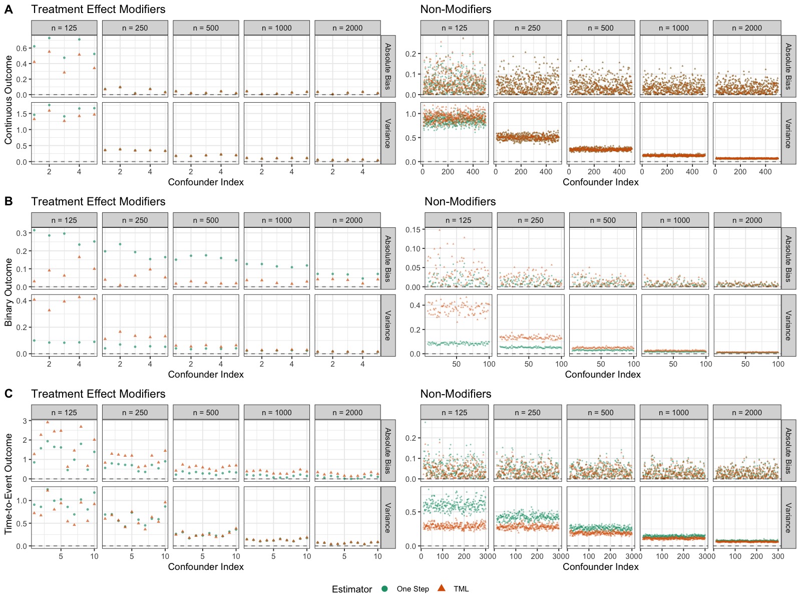
Figure 1A presents the empirical absolute bias and variance of the one-step and TML estimators. Both exhibit a small empirical bias for the TEMs for , but are otherwise approximately unbiased at all other sample sizes. These estimators’ variances are virtually identical at all sample sizes, and rapidly decrease as sample size increases. The bias and variance for non-TEMs (covariates indices 6 to 500) are similarly negligible for both estimators in all sample sizes.
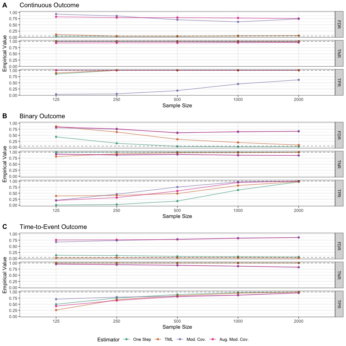
We next evaluate these estimators’ ability to distinguish covariates that modify the effect of treatment from those that do not. The empirical false discovery rate (FDR), true negative rate (TNR), and true positive rate (TPR) are computed at each sample size. The FDR reports the proportion of incorrectly classified covariates among the set of predicted TEMs. The TNR and TPR measure the proportion of correctly classified non-TEMs and TEMs, respectively. Using nominal 5%-level, two-sided Wald-type hypothesis tests and accounting for multiple testing using the FDR-controlling approach of Benjamini and Hochberg (1995), we expect the one-step and TML estimators to achieve a 5% FDR in the largest sample sizes. The one-step and TML estimators’ classification are compared to those of the modified covariates and augmented modified covariates methods. Again, variables with non-zero estimated treatment-covariate interaction coefficients are labeled as TEMs.
Of the four methods considered, only the one-step and TML estimators approximately control the FDR at the nominal level in all sample sizes (Figure 2A). The (augmented) modified covariates methods, on the other hand, maintain an FDR near 75%. Their performance does not improve as a function of . Trends in the methods’ FDRs are elucidated by their TNRs and TPRs. The one-step and TML estimators produce a near-perfect TNR while maintaining a competitive TPR. The augmented modified covariates procedure has a TPR near 100% in all sample sizes, yet has TNRs marginally lower than the one-step and TML estimators. The modified covariates method produces similar TNRs to its augmented counterpart, but has poorer TPRs. The parametric methods’ inability to reliably classify TEMs might be due to the non-linearity of the expected conditional outcome or the number of features relative to the sample size.
6.2 Binary Outcome, Observational Study
We consider another observational DGP, this time with a binary outcome and a moderate number of correlated covariates:
Here, is a Toeplitz matrix, so that the pre-treatment covariates’ correlation structure imitates that of spatial or temporal data. Again, care is taken to avoid practical positivity violation issues.
We benchmark the estimation of the relative TEM-VIP presented in Equation (6). The true parameter values are approximated using Monte Carlo methods. Again, 200 replicates were simulated for each of and . The corresponding one-step and TML estimators are compared and their nuisance parameters are estimated using Super Learners, with the same base learners for and as in the continuous-outcome example. The (augmented) modified covariate methods again rely on the LASSO for propensity score estimation, and use the logistic link function to model the outcome conditional on the potential TEMs and treatment.
The empirical bias and variance of the one-step and TML estimators are provided in Figure 1B. Among the TEMs, the one-step estimator exhibits more finite-sample bias than the TML estimator, though this bias decreases as sample size increases. The TML estimator, however, has noticeably greater finite-sample variance than the one-step for . Among the non-TEMs (pre-treatment covariates indexed 6 through 100), these estimators have similar bias. Again, however, the TML estimator has greater variance in the smaller sample sizes.
The empirical FDR, TNR, and TPR of the one-step and TML estimators, as well as those of the (augmented) modified covariates methods are presented in Figure 2B. Only the one-step estimator reliably controls the FDR at the 5% level at sample sizes of and above. This is seemingly due to the estimator’s conservative behavior: It achieves a near-perfect TNR at all sample sizes, but has the lowest TPR of all estimators regardless of sample size. The TML estimator fails to control the FDR at the desired levels in all sample sizes, though the FDR decreases with sample size and is nearly controlled at . The poor FDR of the TML estimator relative to the one-step estimator may be due to the latter’s increased variability, exhibited in Figure 1B. The (augmented) modified covariates methods tend to perform similarly: their FDR hovers around 75% at all sample sizes, their TNR decreases marginally as increases, and their TPRs are generally higher than those of the nonparametric estimators. Given that sparsity and linearity assumptions are satisfied, the lackluster FDR control of the (augmented) modified covariates procedures might be attributed to violations of the Irrepresentable Condition (Zhao and Yu, 2006) — the covariates’ correlation structure is too complex.
6.3 Right-Censored Time-to-Event Outcome, Randomized Control Trial
Next, we simulate RCT data with known treatment assignment mechanism, a discrete right-censored time-to-event outcome, and a duration of 10 time units. Recall that , where and are defined as before, is the right-censored time-to-event, and is the censoring indicator. The simulation generative model is given by
where the covariates’ covariance matrix is block-diagonal, with each block corresponding to ten moderately correlated features. This correlation structure loosely mimics the expression levels of a collection of genes.
The estimand is defined as the absolute TEM-VIP of Equation (9) at time . Again, the true parameter values are approximated through Monte Carlo methods. The one-step and TML estimators’ conditional censoring hazard function is estimated by the LASSO and their conditional survival hazard function is estimated by the LASSO augmented with treatment-covariate interaction terms. The propensity scores of these nonparametric estimators and the (augmented) modified covariates methods are fixed at , as in a 1:1 RCT. Penalized Cox proportional hazards models are used by the parametric methods to model the conditional survival hazard. We highlight that our simulation DGP satisfies the proportional hazards and non-informative censoring assumptions, but that its covariates possess a complex correlation structure. This might worsen the (augmented) modified covariate methods’ treatment effect modifier classification performance.
Figure 1C presents the one-step and TML estimators’ empirical biases and variances. As for the binary DGP, both estimators are biased for the TEMs (indices 1–10) at all sample sizes, but approximately unbiased for all non-TEMs. As expected, however, the empirical bias associated with the TEMs decreases with sample size, and is negligible when . The empirical variances of these estimators behave as expected, too: they decrease with increasing sample size. The TML estimator’s empirical variances are generally smaller than those of the one-step estimator.
The FDR, TNR, and TPR of all methods considered are reported in Figure 2C. The TML estimator is the only procedure to control the FDR at the nominal 5% level, while the one-step estimator possesses an FDR of approximately 10% for , and which slowly decreases to the nominal rate by . The (augmented) modified covariates approaches result in empirical FDRs that grow with sample size, from approximately 70% for to 90% for . The parametric methods’ behavior with respect to the FDR might be explained by the relationship between their TNR and sample size: as sample size increases, they produce a greater amount of false positives. The nonparametric estimators, however, maintain a near-perfect TNR at all sample sizes. All procedures perform similarly with respect to the TPRs in all but the smallest sample size.
7 Application
We apply our framework to a clinical trial dataset with a right-censored time-to-event outcome. This analysis, as well as the results of the simulation studies, can be reproduced with the code found in this public repository: github.com/PhilBoileau/pub_temvip-framewor.
Trastuzumab is a monoclonal antibody targeting the HER2 oncogene that demonstrably improves the clinical outcomes of breast cancer patients whose tumors over-express this gene. Improvement is not uniform, however: some patients are resistant to this therapy. Identifying biomarkers that predict response to trastuzumab is therefore of great interest (Loi et al., 2014).
Loi et al. (2014) make available a subset of patients enrolled in the FinHER clinical trial (GSE47994), a study comparing docetaxel and vinorelbine — chemotherapies — as adjuvant treatment for early-stage breast cancer (Joensuu et al., 2006). Patients with over-expressed HER2 disease were additionally randomized to receive either nine weekly trastuzumab infusions or no trastuzumab . Loi et al. (2014) provide the quality controlled, normalized gene expression data and relevant clinical information for 201 of these patients. Taking as outcome distant disease-free survival, defined as the time interval between the date of randomization and the date of first cancer recurrence or death, if prior to recurrence, we consider the 500 most variable genes for the purpose of TEM discovery.
Traditional approaches to this task rely on Cox proportional hazards models. For example, a penalized regression of the outcome on the treatment, genes, treatment-gene interactions, and pre-treatment covariates like age and chemotherapy could be fit, and the genes with non-zero estimated interaction coefficients would be classified as TEMs. This is equivalent to the augmented modified covariates approach of Tian et al. (2014). Alternatively, individual regressions for each gene of the outcome conditioning on treatment, gene, pre-treatment covariates, and the treatment-gene interaction could be fitted. Genes with significant treatment-gene interactions would be reported as TEMs. However, both approaches perform inference about conditional parameters, the hazards ratio, while we aim to learn about parameters that reflect population-level information about treatment effect heterogeneity. Verifying the proportional hazards assumption is also impractical given the number of potential TEMs considered.
We instead use our framework, taking as estimand the RMST-based TEM-VIP of Equation (9). Patients’ distant disease-free survival times are discretized into 6-month intervals for computational convenience. We use the TML estimator since the previous simulation experiments suggests that it controls the Type I error rate better than the one-step estimator at this sample size. Its element-wise variance is also likely lower. Given that previous evidence suggests possible higher-order interactions between patients’ chemotherapy regimen, trastuzumab, and biomarkers (Loi et al., 2014), we estimate the conditional failure and censoring hazards using a Super Learner made up of the penalized generalized linear models using the logit link and possessing terms for the treatment, genes, and treatment-gene interactions, Random Forests, and XGBoost (Chen and Guestrin, 2016). This procedures takes approximately 20 minutes to run on a personal computer with a single core of an Apple M1 CPU. Parallelization can reduce this runtime further. We note that similar results are produced by directly estimating the nuisance parameters with Random Forests or XGBoost, though at the expense of an objective choice of nuisance estimators otherwise facilitated by the Super Learner estimator.
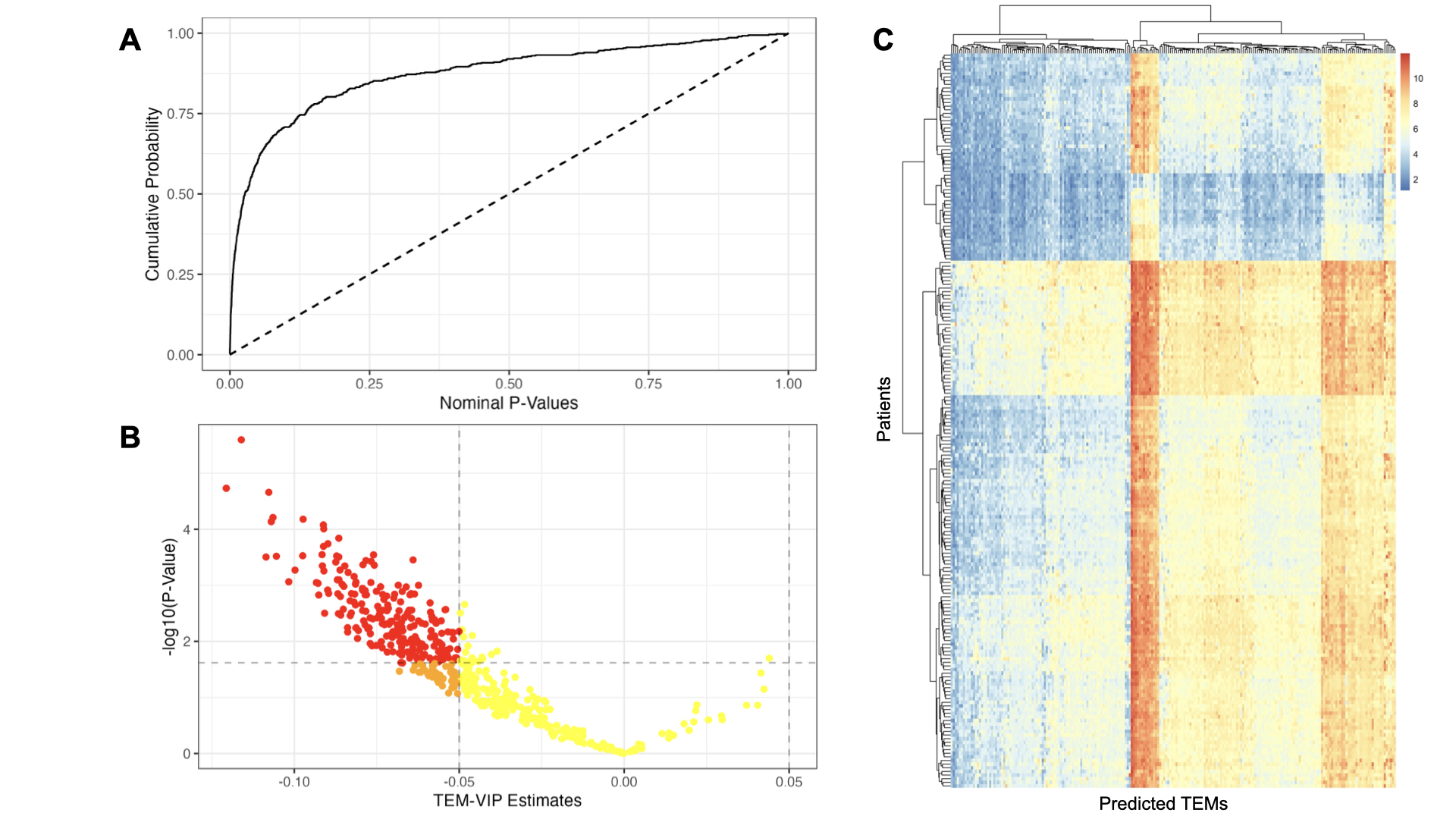
In this analysis, we have sought to dichotomize pre-treatment covariates into TEMs and non-TEMs based on the value of their estimated TEM-VIP. However, as expected, there seems to be a continuum in the biomarkers’ capacity to influence the effect of treatment, in terms of both statistical significance and biological effect size. This can be seen in the empirical cumulative distribution function (eCDF) of the nominal -values (Figure 3A) and in the volcano plot (Figure 3B). Hypothesis testing alone, with a null of , may therefore not be adequate. As in differential expression studies in transcriptomics, one can instead leverage the volcano plot and deem a biomarker of clinical interest if it is significant at the 5% FDR level and if its absolute estimated TEM-VIP is larger than (for each unit increase in log2 gene expression, a TEM-VIP equal to in this analysis approximately corresponds to an expected difference in RMST of about days). There are 220 such biomarkers for the FinHER clinical trial. Alternatively, if one is interested only in modifications above a certain magnitude , one could define the null hypothesis for the biomarker as . The (adjusted) -values obtained from these tests could then be used to produce a ranked list of biomarkers for follow-up analyses. The above considerations highlight the importance of thinking carefully and critically about how to translate the biological question of interest into a statistical inference question, including defining what constitutes a meaningful effect size.
| Gene | Estimate | Std. Err. | Adj. -Value | |
|---|---|---|---|---|
| 1 | EPPK1 | -0.116 | 0.025 | 0.001 |
| 2 | NDUFB3 | -0.121 | 0.028 | 0.004 |
| 3 | BNIP3L | -0.108 | 0.025 | 0.004 |
| 4 | PNKD | -0.106 | 0.027 | 0.006 |
| 5 | DUSP4 | -0.097 | 0.024 | 0.006 |
Now, the five genes with the smallest -values from among the clinically meaningful biomarkers are presented in Table 1. All have previously been linked to breast cancer, and their estimated effects are generally in the direction expected by the literature. Increased EPPK1 expression has been linked to estrogen-related receptor , which is associated with breast cancer growth suppression (Ariazi et al., 2002; Tiraby et al., 2011). A meta-analysis of 11 genome-wide association studies found that a single nucleotide polymorphism in a NDUFB3 promoter was significantly associated estrogen receptor negative breast cancer (Couch et al., 2016). Moussay et al. (2011) found that BNIP3L upregulation is associated with TNF stimulation, which is associated with trastuzumab resistance (Mercogliano et al., 2017). Evidence suggests that overexpression of MR-1S, an isomer of PNKD associated with disordered cell differentiation, malignant transformation initiation, and accelerated metastasis, is therefore a potential therapeutic target of breast cancer (Wang et al., 2018). Finally, Menyhart et al. (2017) found that increased expression of DUSP4 correlates with increased resistance to trastuzumab.
We also present the log-transformed gene expression of the features with clinically meaningful TEM-VIP estimates in Figure 3C. We should expect them to define patient subgroups if these biomarkers truly modify the effect of treatment. Indeed, these genes’ expression data produce multiple distinct patient clusters. We refrain from interpreting Figure 3C any further, however, considering it solely a diagnostic tool. Using patients’ outcomes and biomarkers to compute TEM-VIP estimates, then relying on these estimates to data-adaptively define subgroups in the same data may cause overfitting. These results would ideally be validated on an external dataset, though, as is often the case with openly-accessible clinical trial data, none are available. This might motivate extensions to this TEM discovery framework that support valid inference about both TEM-VIPs and patient subgroups using the same data.
8 Discussion
We propose several causally interpretable TEM-VIPs in full-data models, establish identifiability conditions to relate them to parameters of observed-data distributions, derive accompanying nonparametric estimators, and study these estimators’ asymptotic behavior. Under non-stringent conditions on the DGPs and nuisance parameter estimators, we find that these estimators are consistent. Imposing a few additional assumptions results in efficient, asymptotically linear estimators that permit straightforward hypothesis testing about the corresponding TEM-VIPs. A general workflow for creating new TEM-VIPs and deriving associated nonparametric estimators is provided.
Simulation experiments demonstrate that the estimators’ behavior approximates their established theoretical guarantees in realistic DGPs and for moderate sample sizes. As an additional validation of our methodology, we attempted to identify TEMs in a publicly available clinical trial dataset. These data were originally collected to assess the effect of a monoclonal antibody therapy, trastuzumab, on breast cancer patients. Many genes were classified as TEMs, and a literature review of the top-ranked genes suggests that they are associated with breast cancer. Indeed, a number of these TEMs are known biomarkers of trastuzumab resistance. A diagnostic plot of the predicted TEMs’ expression data further suggests that they may be used to define patient subgroups, but this must be validated with external data.
This work gives rise to several research directions. The framework outlined in Section 5 permits the derivation of bespoke pathwise differentiable TEM-VIPs and accompanying nonparametric efficient estimators. In particular, researchers working in the biotechnology and pharmaceutical industries can perform inference about TEM-VIPs derived from estimands used in clinical trials. Such heterogeneous treatment effect analyses would closely track the statistical guidelines enforced by regulatory authorities, like those of the International Council for Harmonization of Technical Requirements for Pharmaceuticals for Human Use for clinical trials (International Council for Harmonisation of Technical Requirements for Pharmaceuticals for Human Use, 2019). This framework for TEM inference might also support statistically rigorous subgroup discovery. TEMs identified using our methodology could be used to cluster observations (i.e., patients), and, subsequently, treatment effects could be estimated within these groups. Whether there exists a sound approach that permits the application of this workflow to a single dataset, perhaps building on recent advances in post-selection inference, should be investigated. Future work might also determine whether these TEM-VIP estimators improve treatment rule estimation procedures by acting as variable filters. That is, only pre-treatment covariates with TEM-VIP estimates significantly different from zero would be used, along with known confounders, to learn the treatment rule. Doing so would increase the interpretability of the rule and might improve estimation in high-dimensional regimes.
Appendix
S1 Proofs
Theorem 1
Proposition 1
Proof.
Proposition 2
Proof.
From the definition of given by Equation (5), we find that
It follows immediately that when or for . ∎
Theorem 2
Proof.
Asymptotic linearity of and are achieved when the third and fourth terms in the von Mises expansion of Equation (3) converge in probability to 0. Under A7, with probability tending to one which implies that . It follows that the third term of the von Mises expansion is .
What remains is to bound the error term. From Boileau et al. (2022), we find that
The last inequality follows from A9. A similar bound applies to . The remainder term of Equation (3) is therefore under the conditions of A8.
It follows, applying the central limit theorem to the first term of the von Mises expansion, that . The same is true for .
∎
Corollary 1
Proof.
The conditions outlined in Theorem 1 imply that . It follows immediately that is equal to . ∎
Proposition 3
Proof.
Using the same point mass contamination approach, we obtain the following efficient influence function for :
∎
Proposition 4
Proof.
Theorem 3
Proof.
The proof is analogous to Theorem 2. Again, the entropy constraint of A7 ensures that the third term of the von Mises expansion converges to zero in probability to 1. The remainder term in the same von Mises expansion is shown to be :
The second equality follows from A10 and the Maclaurin series of . The final inequality follows from A9 and that is a positive random variable such that almost surely (a.s.). The reported result follows by applying the central limit theorem to the first term of the von Mises expansion.
∎
Theorem 4
Proposition 5
Proof.
Using previous results from Moore and van der Laan (2011) and the functional delta method, we obtain:
∎
Proposition 6
Proof.
Theorem 5
Proof.
The proof is analogous Theorem 2’s. From the results of Moore and van der Laan (2011) and the the functional delta method, the entropy condition of A7 implies that the third term of the von Mises expansion for any given is . Then,
Similar to the proof of Proposition 6, it suffices to show that the integrand is bounded by . Indeed, this has previously been established under conditions A7, A2, A9, A16 and A17. See, for example, van der Laan and Robins (2003), (Tsiatis, 2006) and Cui et al. (2022). ∎
Corollary 2
Proof.
It follows from the conditions of Theorem 4 that is equal to . ∎
Proposition 7
Proof.
Again relying on the point mass contamination approach, we obtain:
∎
Proposition 8
Theorem 6
Proof.
Again, the entropy condition of A7 implies that the third term of the von Mises expansion is . Studying the remainder term, we find that
The stated result follows.
∎
References
- Hernán [2010] Miguel A. Hernán. The hazards of hazard ratios. Epidemiology, 21(1), 2010.
- Greenland et al. [1999] Sander Greenland, Judea Pearl, and James M. Robins. Confounding and Collapsibility in Causal Inference. Statistical Science, 14(1):29 – 46, 1999.
- Rubin [1974] D.B. Rubin. Estimating causal effects of treatments in randomized and nonrandomized studies. Journal of Educational Psychology, 66(5):688–701, 1974.
- Zhao et al. [2018] Qingyuan Zhao, Dylan S. Small, and Ashkan Ertefaie. Selective inference for effect modification via the LASSO, 2018.
- Semenova and Chernozhukov [2020] Vira Semenova and Victor Chernozhukov. Debiased machine learning of conditional average treatment effects and other causal functions. The Econometrics Journal, 24(2):264–289, 08 2020. ISSN 1368-4221. doi: 10.1093/ectj/utaa027. URL https://doi.org/10.1093/ectj/utaa027.
- Bahamyirou et al. [2022] Asma Bahamyirou, Mireille E. Schnitzer, Edward H. Kennedy, Lucie Blais, and Yi Yang. Doubly robust adaptive LASSO for effect modifier discovery. The International Journal of Biostatistics, 2022. doi: doi:10.1515/ijb-2020-0073. URL https://doi.org/10.1515/ijb-2020-0073.
- van der Laan et al. [2007] Mark J. van der Laan, Eric C. Polley, and Alan E. Hubbard. Super Learner. Statistical Applications in Genetics and Molecular Biology, 6(1), 2007. doi: doi:10.2202/1544-6115.1309. URL https://doi.org/10.2202/1544-6115.1309.
- Luedtke and van der Laan [2016] Alexander R. Luedtke and Mark J. van der Laan. Super-learning of an optimal dynamic treatment rule. The International Journal of Biostatistics, 12(1):305–332, 2016. doi: doi:10.1515/ijb-2015-0052. URL https://doi.org/10.1515/ijb-2015-0052.
- Breiman [2001] Leo Breiman. Random Forests. Machine Learning, 45(1):5–32, 2001.
- Wager and Athey [2018] Stefan Wager and Susan Athey. Estimation and inference of heterogeneous treatment effects using Random Forests. Journal of the American Statistical Association, 113(523):1228–1242, 2018. doi: 10.1080/01621459.2017.1319839. URL https://doi.org/10.1080/01621459.2017.1319839.
- Cui et al. [2022] Yifan Cui, Michael R. Kosorok, Erik Sverdrup, Stefan Wager, and Ruoqing Zhu. Estimating heterogeneous treatment effects with right-censored data via causal Survival Forests, 2022. URL https://arxiv.org/abs/2001.09887.
- Tibshirani [1996] Robert Tibshirani. Regression shrinkage and selection via the Lasso. Journal of the Royal Statistical Society. Series B (Methodological), 58(1):267–288, 1996. ISSN 00359246. URL http://www.jstor.org/stable/2346178.
- Tian et al. [2014] Lu Tian, Ash A. Alizadeh, Andrew J. Gentles, and Robert Tibshirani. A simple method for estimating interactions between a treatment and a large number of covariates. Journal of the American Statistical Association, 109(508):1517–1532, 2014. doi: 10.1080/01621459.2014.951443. URL https://doi.org/10.1080/01621459.2014.951443. PMID: 25729117.
- Chen and Guestrin [2016] Tianqi Chen and Carlos Guestrin. XGBoost: A scalable tree boosting system. In Proceedings of the 22nd ACM SIGKDD International Conference on Knowledge Discovery and Data Mining, KDD ’16, pages 785–794, New York, NY, USA, 2016. ACM. ISBN 978-1-4503-4232-2. doi: 10.1145/2939672.2939785. URL http://doi.acm.org/10.1145/2939672.2939785.
- Zhao and Yu [2006] Peng Zhao and Bin Yu. On model selection consistency of Lasso. Journal of Machine Learning Research, 7(90):2541–2563, 2006. URL http://jmlr.org/papers/v7/zhao06a.html.
- Hastie et al. [2009] Trevor Hastie, Robert Tibshirani, and Jerome Friedman. The elements of statistical learning: Data mining, inference and prediction. Springer, 2 edition, 2009. URL http://www-stat.stanford.edu/~tibs/ElemStatLearn/.
- Williamson et al. [2022] Brian D. Williamson, Peter B. Gilbert, Noah R. Simon, and Marco Carone. A general framework for inference on algorithm-agnostic variable importance. Journal of the American Statistical Association, 0(0):1–14, 2022.
- Boileau et al. [2022] Philippe Boileau, Nina Ting Qi, Mark J. van der Laan, Sandrine Dudoit, and Ning Leng. A flexible approach for predictive biomarker discovery. Biostatistics, 07 2022. ISSN 1465-4644. doi: 10.1093/biostatistics/kxac029. URL https://doi.org/10.1093/biostatistics/kxac029. kxac029.
- Hines et al. [2022a] Oliver Hines, Karla Diaz-Ordaz, and Stijn Vansteelandt. Variable importance measures for heterogeneous causal effects, 2022a. URL https://arxiv.org/abs/2204.06030.
- Levy et al. [2021] Jonathan Levy, Mark van der Laan, Alan Hubbard, and Romain Pirracchio. A fundamental measure of treatment effect heterogeneity. Journal of Causal Inference, 9(1):83–108, 2021.
- Rosenblum and van der Laan [2010] Michael Rosenblum and Mark J. van der Laan. Simple, efficient estimators of treatment effects in randomized trials using generalized linear models to leverage baseline variables. The International Journal of Biostatistics, 6(1), 2010.
- Tchetgen Tchetgen et al. [2009] Eric J. Tchetgen Tchetgen, James M. Robins, and Andrea Rotnitzky. On doubly robust estimation in a semiparametric odds ratio model. Biometrika, 97(1):171–180, 12 2009. ISSN 0006-3444. doi: 10.1093/biomet/asp062. URL https://doi.org/10.1093/biomet/asp062.
- Tuglus et al. [2011] Cathy Tuglus, Kristin E. Porter, and Mark J. van der Laan. Targeted maximum likelihood estimation of conditional relative risk in a semi-parametric regression model. Working Paper 283, University of California, Berkeley, Berkeley, 2011. URL https://biostats.bepress.com/ucbbiostat/paper283/.
- Chambaz et al. [2012] Antoine Chambaz, Pierre Neuvial, and Mark J. van der Laan. Estimation of a non-parametric variable importance measure of a continuous exposure. Electronic Journal of Statistics, 6(none):1059 – 1099, 2012.
- Yadlowsky et al. [2021] Steve Yadlowsky, Fabio Pellegrini, Federica Lionetto, Stefan Braune, and Lu Tian. Estimation and validation of ratio-based conditional average treatment effects using observational data. Journal of the American Statistical Association, 116(533):335–352, 2021.
- Chen et al. [2017] Shuai Chen, Lu Tian, Tianxi Cai, and Menggang Yu. A general statistical framework for subgroup identification and comparative treatment scoring. Biometrics, 73(4):1199–1209, 2017. doi: https://doi.org/10.1111/biom.12676. URL https://onlinelibrary.wiley.com/doi/abs/10.1111/biom.12676.
- Ning et al. [2020] Yang Ning, Peng Sida, and Kosuke Imai. Robust estimation of causal effects via a high-dimensional covariate balancing propensity score. Biometrika, 107(3):533–554, 06 2020. ISSN 0006-3444. doi: 10.1093/biomet/asaa020. URL https://doi.org/10.1093/biomet/asaa020.
- Fisher and Kennedy [2021] Aaron Fisher and Edward H. Kennedy. Visually communicating and teaching intuition for influence functions. The American Statistician, 75(2):162–172, 2021.
- Hines et al. [2022b] Oliver Hines, Oliver Dukes, Karla Diaz-Ordaz, and Stijn Vansteelandt. Demystifying statistical learning based on efficient influence functions. The American Statistician, 0(ja):1–48, 2022b. doi: 10.1080/00031305.2021.2021984. URL https://doi.org/10.1080/00031305.2021.2021984.
- von Mises [1947] Richard von Mises. On the asymptotic distribution of differentiable statistical functions. The Annals of Mathematical Statistics, 18(3):309–348, 1947.
- Bickel et al. [1993] Peter J. Bickel, Chris A. J. Klaassen, YA’Acov Ritov, and Jon A. Wellner. Efficient and adaptive estimation for semiparametric models. Johns Hopkins University Press Baltimore, 1993.
- van der Laan and Robins [2003] Mark J. van der Laan and James M. Robins. Unified Methods for Censored Longitudinal Data and Causality. Springer Science & Business Media, 2003.
- Pfanzagl and Wefelmeyer [1985] Johann Pfanzagl and Wolfgang Wefelmeyer. Contributions to a general asymptotic statistical theory. Statistics & Risk Modeling, 3(3-4):379–388, 1985.
- Klaassen [1987] Chris A. J. Klaassen. Consistent estimation of the influence function of locally asymptotically linear estimators. The Annals of Statistics, 15(4):1548–1562, 1987. ISSN 00905364. URL http://www.jstor.org/stable/2241690.
- Zheng and van der Laan [2011] Wenjing Zheng and Mark J. van der Laan. Cross-validated targeted minimum-loss-based estimation. In Targeted Learning: Causal Inference for Observational and Experimental Data, pages 459–474. Springer, 2011.
- Chernozhukov et al. [2017] Victor Chernozhukov, Denis Chetverikov, Mert Demirer, Esther Duflo, Christian Hansen, and Whitney Newey. Double/debiased/neyman machine learning of treatment effects. American Economic Review, 107(5):261–65, May 2017. doi: 10.1257/aer.p20171038. URL https://www.aeaweb.org/articles?id=10.1257/aer.p20171038.
- van der Laan and Rubin [2006] Mark J. van der Laan and Daniel Rubin. Targeted maximum likelihood learning. International Journal of Biostatistics, 2(1), 2006.
- van der Laan and Rose [2011] Mark J. van der Laan and Sherri Rose. Targeted Learning: Causal Inference for Observational and Experimental Data. Springer Science & Business Media, 2011.
- van der Laan and Rose [2018] Mark J. van der Laan and Sherri Rose. Targeted Learning in Data Science: Causal Inference for Complex Longitudinal Data. Springer International Publishing, 2018.
- Tsiatis [2006] Anastasios Tsiatis. Semiparametric Theory and Missing Data. Springer Series in Statistics. Springer New York, New York, NY, 1st ed. 2006. edition, 2006.
- Hejazi et al. [2023] Nima S. Hejazi, Philippe Boileau, Mark J. van der Laan, and Alan E. Hubbard. A generalization of moderated statistics to data adaptive semiparametric estimation in high-dimensional biology, 2023.
- Gruber and van der Laan [2010] Susan Gruber and Mark J. van der Laan. A targeted maximum likelihood estimator of a causal effect on a bounded continuous outcome. The International Journal of Biostatistics, 6(1), 2010.
- Bickel and Doksum [2015] Peter J. Bickel and Kjell A. Doksum. Mathematical Statistics: Basic Ideas and Selected Topics, volume II. Chapman and and Hall, CRC Press, 2015. doi: 10.1201/9781315369266.
- Neuhaus [1971] Georg Neuhaus. On Weak Convergence of Stochastic Processes with Multidimensional Time Parameter. The Annals of Mathematical Statistics, 42(4):1285 – 1295, 1971.
- Gill et al. [1995] Richard D. Gill, Mark J. Laan, and Jon A. Wellner. Inefficient estimators of the bivariate survival function for three models. In Annales de l’IHP Probabilités et statistiques, volume 31, pages 545–597, 1995.
- van der Laan and Gruber [2016] Mark van der Laan and Susan Gruber. The International Journal of Biostatistics, 12(1):351–378, 2016.
- van der Laan [2017] Mark van der Laan. A generally efficient targeted minimum loss based estimator based on the highly adaptive lasso. The International Journal of Biostatistics, 13(2):20150097, 2017. doi: doi:10.1515/ijb-2015-0097. URL https://doi.org/10.1515/ijb-2015-0097.
- Bickel [1982] P. J. Bickel. On Adaptive Estimation. The Annals of Statistics, 10(3):647 – 671, 1982.
- Schick [1986] Anton Schick. On Asymptotically Efficient Estimation in Semiparametric Models. The Annals of Statistics, 14(3):1139 – 1151, 1986.
- Farrell et al. [2021] Max H. Farrell, Tengyuan Liang, and Sanjog Misra. Deep neural networks for estimation and inference. Econometrica, 89(1):181–213, 2021. doi: https://doi.org/10.3982/ECTA16901. URL https://onlinelibrary.wiley.com/doi/abs/10.3982/ECTA16901.
- Bibaut and van der Laan [2019] Aurélien F. Bibaut and Mark J. van der Laan. Fast rates for empirical risk minimization over càdlàg functions with bounded sectional variation norm, 2019. URL https://arxiv.org/abs/1907.09244.
- Chen and Tsiatis [2001] Pei-Yun Chen and Anastasios A. Tsiatis. Causal inference on the difference of the restricted mean lifetime between two groups. Biometrics, 57(4):1030–1038, 2001.
- Royston and Parmar [2011] Patrick Royston and Mahesh K. B. Parmar. The use of restricted mean survival time to estimate the treatment effect in randomized clinical trials when the proportional hazards assumption is in doubt. Statistics in Medicine, 30(19):2409–2421, 2011. doi: https://doi.org/10.1002/sim.4274. URL https://onlinelibrary.wiley.com/doi/abs/10.1002/sim.4274.
- Díaz et al. [2019] Iván Díaz, Elizabeth Colantuoni, Daniel F. Hanley, and Michael Rosenblum. Improved precision in the analysis of randomized trials with survival outcomes, without assuming proportional hazards. Lifetime Data Analysis, 25(3):439–468, 2019.
- Moore and van der Laan [2011] Kelly Moore and Mark van der Laan. RCTs with Time-to-Event Outcomes, pages 259–269. 06 2011. ISBN 978-1-4419-9781-4. doi: 10.1007/978-1-4419-9782-1_17.
- Benkeser et al. [2019] David Benkeser, Peter B. Gilbert, and Marco Carone. Estimating and testing vaccine sieve effects using machine learning. Journal of the American Statistical Association, 114(527):1038–1049, 2019.
- R Core Team [2023] R Core Team. R: A Language and Environment for Statistical Computing. R Foundation for Statistical Computing, Vienna, Austria, 2023. URL https://www.R-project.org/.
- Duncan and Tang [2022] James Duncan and Tiffany Tang. simChef: Intensive Computational Experiments Made Easy, 2022. URL https://yu-group.github.io/simChef. R package version 0.0.2.
- Huling and Yu [2021] Jared D. Huling and Menggang Yu. Subgroup identification using the personalized package. Journal of Statistical Software, 98(5):1–60, 2021. doi: 10.18637/jss.v098.i05. URL https://www.jstatsoft.org/index.php/jss/article/view/v098i05.
- Coyle et al. [2021] Jeremy R Coyle, Nima S Hejazi, Ivana Malenica, Rachael V Phillips, and Oleg Sofrygin. sl3: Modern Pipelines for Machine Learning and Super Learning, 2021. URL https://doi.org/10.5281/zenodo.1342293. R package version 1.4.2.
- Zou and Hastie [2005] Hui Zou and Trevor Hastie. Regularization and variable selection via the elastic net. Journal of the Royal Statistical Society. Series B (Statistical Methodology), 67(2):301–320, 2005. ISSN 13697412, 14679868. URL http://www.jstor.org/stable/3647580.
- Friedman [1991] Jerome H. Friedman. Multivariate Adaptive Regression Splines. The Annals of Statistics, 19(1):1 – 67, 1991.
- Benjamini and Hochberg [1995] Yoav Benjamini and Yosef Hochberg. Controlling the false discovery rate: A practical and powerful approach to multiple testing. Journal of the Royal Statistical Society. Series B (Methodological), 57(1):289–300, 1995. ISSN 00359246. URL http://www.jstor.org/stable/2346101.
- Loi et al. [2014] S. Loi, S. Michiels, R. Salgado, N. Sirtaine, V. Jose, D. Fumagalli, P.-L. Kellokumpu-Lehtinen, P. Bono, V. Kataja, C. Desmedt, M.J. Piccart, S. Loibl, C. Denkert, M.J. Smyth, H. Joensuu, and C. Sotiriou. Tumor infiltrating lymphocytes are prognostic in triple negative breast cancer and predictive for trastuzumab benefit in early breast cancer: Results from the FinHER trial. Annals of Oncology, 25(8):1544–1550, 2014.
- Joensuu et al. [2006] Heikki Joensuu, Pirkko-Liisa Kellokumpu-Lehtinen, Petri Bono, Tuomo Alanko, Vesa Kataja, Raija Asola, Tapio Utriainen, Riitta Kokko, Akseli Hemminki, Maija Tarkkanen, Taina Turpeenniemi-Hujanen, Sirkku Jyrkkiö, Martti Flander, Leena Helle, Seija Ingalsuo, Kaisu Johansson, Anna-Stina Jääskeläinen, Marjo Pajunen, Mervi Rauhala, Jaana Kaleva-Kerola, Tapio Salminen, Mika Leinonen, Inkeri Elomaa, and Jorma Isola. Adjuvant docetaxel or vinorelbine with or without trastuzumab for breast cancer. New England Journal of Medicine, 354(8):809–820, 2006.
- Ariazi et al. [2002] Eric A. Ariazi, Gary M. Clark, and Janet E. Mertz. Estrogen-related Receptor \textalphaand Estrogen-related Receptor \textgammaAssociate with Unfavorable and Favorable Biomarkers, Respectively, in Human Breast Cancer1. Cancer Research, 62(22):6510–6518, 11 2002. ISSN 0008-5472.
- Tiraby et al. [2011] Claire Tiraby, Bethany C. Hazen, Marin L. Gantner, and Anastasia Kralli. Estrogen-Related Receptor \textgammaPromotes Mesenchymal-to-Epithelial Transition and Suppresses Breast Tumor Growth. Cancer Research, 71(7):2518–2528, 03 2011. ISSN 0008-5472. doi: 10.1158/0008-5472.CAN-10-1315. URL https://doi.org/10.1158/0008-5472.CAN-10-1315.
- Couch et al. [2016] Fergus J. Couch, Karoline B. Kuchenbaecker, Kyriaki Michailidou, Gustavo A. Mendoza-Fandino, Silje Nord, Janna Lilyquist, Curtis Olswold, Emily Hallberg, Simona Agata, Habibul Ahsan, Kristiina Aittomäki, Christine Ambrosone, Irene L. Andrulis, Hoda Anton-Culver, Volker Arndt, Banu K. Arun, Brita Arver, Monica Barile, Rosa B. Barkardottir, Daniel Barrowdale, Lars Beckmann, Matthias W. Beckmann, Javier Benitez, Stephanie V. Blank, Carl Blomqvist, Natalia V. Bogdanova, Stig E. Bojesen, Manjeet K. Bolla, Bernardo Bonanni, Hiltrud Brauch, Hermann Brenner, Barbara Burwinkel, Saundra S. Buys, Trinidad Caldes, Maria A. Caligo, Federico Canzian, Jane Carpenter, Jenny Chang-Claude, Stephen J. Chanock, Wendy K. Chung, Kathleen B. M. Claes, Angela Cox, Simon S. Cross, Julie M. Cunningham, Kamila Czene, Mary B. Daly, Francesca Damiola, Hatef Darabi, Miguel de la Hoya, Peter Devilee, Orland Diez, Yuan C. Ding, Riccardo Dolcetti, Susan M. Domchek, Cecilia M. Dorfling, Isabel dos Santos-Silva, Martine Dumont, Alison M. Dunning, Diana M. Eccles, Hans Ehrencrona, Arif B. Ekici, Heather Eliassen, Steve Ellis, Peter A. Fasching, Jonine Figueroa, Dieter Flesch-Janys, Asta Försti, Florentia Fostira, William D. Foulkes, Tara Friebel, Eitan Friedman, Debra Frost, Marike Gabrielson, Marilie D. Gammon, Patricia A. Ganz, Susan M. Gapstur, Judy Garber, Mia M. Gaudet, Simon A. Gayther, Anne-Marie Gerdes, Maya Ghoussaini, Graham G. Giles, Gord Glendon, Andrew K. Godwin, Mark S. Goldberg, David E. Goldgar, Anna González-Neira, Mark H. Greene, Jacek Gronwald, Pascal Guénel, Marc Gunter, Lothar Haeberle, Christopher A. Haiman, Ute Hamann, Thomas V. O. Hansen, Steven Hart, Sue Healey, Tuomas Heikkinen, Brian E. Henderson, Josef Herzog, Frans B. L. Hogervorst, Antoinette Hollestelle, Maartje J. Hooning, Robert N. Hoover, John L. Hopper, Keith Humphreys, David J. Hunter, Tomasz Huzarski, Evgeny N. Imyanitov, Claudine Isaacs, Anna Jakubowska, Paul James, Ramunas Janavicius, Uffe Birk Jensen, Esther M. John, Michael Jones, Maria Kabisch, Siddhartha Kar, Beth Y. Karlan, Sofia Khan, Kay-Tee Khaw, Muhammad G. Kibriya, Julia A. Knight, Yon-Dschun Ko, Irene Konstantopoulou, Veli-Matti Kosma, Vessela Kristensen, Ava Kwong, Yael Laitman, Diether Lambrechts, Conxi Lazaro, Eunjung Lee, Loic Le Marchand, Jenny Lester, Annika Lindblom, Noralane Lindor, Sara Lindstrom, Jianjun Liu, Jirong Long, Jan Lubinski, Phuong L. Mai, Enes Makalic, Kathleen E. Malone, Arto Mannermaa, Siranoush Manoukian, Sara Margolin, Frederik Marme, John W. M. Martens, Lesley McGuffog, Alfons Meindl, Austin Miller, Roger L. Milne, Penelope Miron, Marco Montagna, Sylvie Mazoyer, Anna M. Mulligan, Taru A. Muranen, Katherine L. Nathanson, Susan L. Neuhausen, Heli Nevanlinna, Børge G. Nordestgaard, Robert L. Nussbaum, Kenneth Offit, Edith Olah, Olufunmilayo I. Olopade, Janet E. Olson, Ana Osorio, Sue K. Park, Petra H. Peeters, Bernard Peissel, Paolo Peterlongo, Julian Peto, Catherine M. Phelan, Robert Pilarski, Bruce Poppe, Katri Pylkäs, Paolo Radice, Nazneen Rahman, Johanna Rantala, Christine Rappaport, Gad Rennert, Andrea Richardson, Mark Robson, Isabelle Romieu, Anja Rudolph, Emiel J. Rutgers, Maria-Jose Sanchez, Regina M. Santella, Elinor J. Sawyer, Daniel F. Schmidt, Marjanka K. Schmidt, Rita K. Schmutzler, Fredrick Schumacher, Rodney Scott, Leigha Senter, Priyanka Sharma, Jacques Simard, Christian F. Singer, Olga M. Sinilnikova, Penny Soucy, Melissa Southey, Doris Steinemann, Marie Stenmark-Askmalm, Dominique Stoppa-Lyonnet, Anthony Swerdlow, Csilla I. Szabo, Rulla Tamimi, William Tapper, Manuel R. Teixeira, Soo-Hwang Teo, Mary B. Terry, Mads Thomassen, Deborah Thompson, Laima Tihomirova, Amanda E. Toland, Robert A. E. M. Tollenaar, Ian Tomlinson, Thérèse Truong, Helen Tsimiklis, Alex Teulé, Rosario Tumino, Nadine Tung, Clare Turnbull, Giski Ursin, Carolien H. M. van Deurzen, Elizabeth J. van Rensburg, Raymonda Varon-Mateeva, Zhaoming Wang, Shan Wang-Gohrke, Elisabete Weiderpass, Jeffrey N. Weitzel, Alice Whittemore, Hans Wildiers, Robert Winqvist, Xiaohong R. Yang, Drakoulis Yannoukakos, Song Yao, M Pilar Zamora, Wei Zheng, Per Hall, Peter Kraft, Celine Vachon, Susan Slager, Georgia Chenevix-Trench, Paul D. P. Pharoah, Alvaro A. N. Monteiro, Montserrat García-Closas, Douglas F. Easton, and Antonis C. Antoniou. Identification of four novel susceptibility loci for oestrogen receptor negative breast cancer. Nature Communications, 7(1):11375, 2016.
- Moussay et al. [2011] Etienne Moussay, Tony Kaoma, Joanna Baginska, Arnaud Muller, Kris Van Moer, Nathalie Nicot, Petr V. Nazarov, Laurent Vallar, Salem Chouaib, Guy Berchem, and Bassam Janji. The acquisition of resistance to TNF\textalphain breast cancer cells is associated with constitutive activation of autophagy as revealed by a transcriptome analysis using a custom microarray. Autophagy, 7(7):760–770, 2011.
- Mercogliano et al. [2017] María F. Mercogliano, Mara De Martino, Leandro Venturutti, Martín A. Rivas, Cecilia J. Proietti, Gloria Inurrigarro, Isabel Frahm, Daniel H. Allemand, Ernesto Gil Deza, Sandra Ares, Felipe G. Gercovich, Pablo Guzmán, Juan C. Roa, Patricia V. Elizalde, and Roxana Schillaci. TNF\textalpha-Induced Mucin 4 Expression Elicits Trastuzumab Resistance in HER2-Positive Breast Cancer. Clinical Cancer Research, 23(3):636–648, 01 2017. ISSN 1078-0432. doi: 10.1158/1078-0432.CCR-16-0970. URL https://doi.org/10.1158/1078-0432.CCR-16-0970.
- Wang et al. [2018] Junxia Wang, Wuli Zhao, Hong Liu, Hongwei He, and Rongguang Shao. Myofibrillogenesis regulator 1 (MR-1): a potential therapeutic target for cancer and PNKD. Journal of Drug Targeting, 26(8):643–648, 2018.
- Menyhart et al. [2017] Otília Menyhart, Jan Budczies, Gyöngyi Munkácsy, Francisco J Esteva, András Szabó, Teresa Puig Miquel, and Balázs Győrffy. DUSP4 is associated with increased resistance against anti-HER2 therapy in breast cancer. Oncotarget, 8(44):77207–77218, 2017. ISSN 1949-2553. doi: https://doi.org/10.18632/oncotarget.20430. URL https://www.oncotarget.com/article/20430/.
- International Council for Harmonisation of Technical Requirements for Pharmaceuticals for Human Use [2019] International Council for Harmonisation of Technical Requirements for Pharmaceuticals for Human Use. Addendum on estimands and sensitivity analysis in clinical trials to the guideline on statistical principles for clinical trials E9(R1). https://database.ich.org/sites/default/files/E9-R1_Step4_Guideline_2019_1203.pdf, 2019. Accessed: 2023-01-24.