Identification of nonlinear beam-hardening effects in X-ray tomography

Abstract.

We study streaking artifacts caused by beam-hardening effects in X-ray computed tomography (CT). The effect is known to be nonlinear. We show that the nonlinearity can be recovered from the observed artifacts for strictly convex bodies. The result provides a theoretical support for removal of the artifacts.

1. Introduction

In X-ray computed tomography (CT), artifacts due to beam-hardening effects is common for patients with medical implants. They are notorious for causing degradation of CT images and difficulties for diagnosis. The reduction or removal of such artifacts has drawn numerous research efforts, but the problem still remains one of the major challenges in X-ray CT.

In [11], the authors demonstrated the nonlinear nature of the beam-hardening effects. Let $f$ be the attenuation coefficient of the object being imaged. Because of the polychromatic nature of X-ray beams, we consider the dependency of $f$ on the energy level $E$. This is particularly significant for metal objects. Assume that $E\in[E_{0}-\epsilon,E_{0}+\epsilon]$, $\epsilon>0$, and write $f$ as $f_{E}$. We write $f_{E}(x)=f_{E_{0}}(x)+\alpha\chi_{D}$, where $\chi_{D}$ is the characteristic function for a metal object $D\subset{\mathbb{R}}^{2}$, and $\alpha>0$ a constant which can be thought of as the approximation of the derivative of $f_{E}$ in $E$. The X-ray data can be derived from the Beer-Lambert law which gives

(1) $$P=Rf_{E}+P_{MA}.$$

Here, $Rf_{E}$ denote the Radon transform of $f_{E}$, and $P_{MA}$ denotes a mismatch term. Under further assumptions, it is derived in [11] that

(2) $$P_{MA}=-\ln\left(\frac{\sinh(\alpha\epsilon R\chi_{D})}{\alpha\epsilon R\chi_{D}}\right)$$

is a nonlinear function of $R\chi_{D}$. If one applies the filtered back-projection (FBP) to reconstruct $f_{E}$, the mismatch term $P_{MA}$ leads to the artifact, see Figure 1 for a demonstration. By using the notion of wave front set in microlocal analysis, the authors of [11] gave a mathematical characterization of the artifacts. For strictly convex objects, the artifacts appear to be straight lines tangent to at least two boundary points of the metal objects, see Figure 1. For more complicated situations, the artifacts and their relation to the geometry of metal regions are further studied in [10, 17]. Finally, we mention that artifacts due to similar mechanism are also known in the attenuated X-ray tomography, see [7].

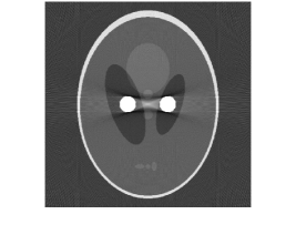
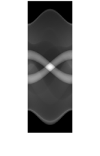
Figure 1. Illustration of the beam-hardening artifacts produced by a quadratic nonlinearity. The left figure shows the reconstruction from FBP. The two bright disks represents the metal objects. The artifacts appear to be straight lines tangent to both disks. The right figure shows the sinogram (color map of $P$ in (1)). The two bright strips correspond to the support of $R\chi_{D}.$

The identification of the nonlinear effect in $P_{MA}$ is the key for removal of the artifacts. In practice, the shape of the metal objects can usually be acquired so it is reasonable to assume that $\chi_{D}$ is known and think of $P_{MA}$ as a nonlinear function $F(R{\chi_{D}})$. Then one can remove $P_{MA}$ if $F$ is known. For example, the numerical scheme developed in [12] consists of two steps: first, one recovers $\chi_{D}$ from the reconstruction $f_{CT}$ using image segmentation techniques; second, one can use the model (2) and find the optimal $\alpha$ which reduces the artifact. In general, not much can be said about the nonlinear function as it depends on many factors such as the energy distribution of X-ray beams, geometry and physical properties of metal objects and even $f_{E_{0}}$. Lately, there have been increasing efforts to find the nonlinear effect by using deep learning techniques, see for example [13, 18].

The purpose of this note is to show that the nonlinearity can be identified from the observed artifacts. Also, we provide a constructive proof which is potentially useful in practice.

2. The main result

Because of the local nature of the problem as we explain later, it suffices to state our main result in a relatively simple setting. We assume that the metal region $D=D_{1}\cup D_{2}$, where $D_{j},j=1,2$ are simply connected disjoint bounded domains in ${\mathbb{R}}^{2}$ with smooth boundary $\partial D_{j}$. Let $\chi_{D}=\chi_{D_{1}}+\chi_{D_{2}}$ be the characteristic function of $D$. We assume that the attenuation coefficient is of the form

(3) $$f(x)=h(x)+\chi_{D}(x),\quad x\in{\mathbb{R}}^{2}$$

where $h$ represents the attenuation coefficient of the tissue. For the Radon transform on ${\mathbb{R}}^{2}$, we use the following parametrization

$$Rf(s,\phi)=\int_{x_{1}\cos\phi+x_{2}\sin\phi=s}f(x)dx$$

Here, $x\in{\mathbb{R}}$ and $(s,\phi)\in M={\mathbb{R}}\times(-\pi,\pi)$. Note that because we are dealing with a local problem for $Rf$, it suffices to use local coordinates in the region of interest. We model the beam-hardening effects by a polynomial function $F:{\mathbb{C}}\rightarrow{\mathbb{C}}$ of the form

(4) $$F(t)=\sum_{j=2}^{J}a_{j}t^{j}$$

where $a_{j}$ are constant and $J\in{\mathbb{N}}.$ Then the X-ray CT data is modeled by

(5) $$P=Rf+P_{MA},\quad P_{MA}=F(R\chi_{D})$$

For the reconstruction, we apply the FBP to get

(6) $$f_{CT}=f+f_{MA},\ \ f_{MA}=R^{*}I^{-1}P_{MA}$$

where $I^{-1}$ is the Riesz potential and $R^{*}$ denotes the adjoint of $R$, see for example [15]. Our main result is

Theorem 2.1.

Suppose $D_{j},j=1,2$ are strictly convex and $h\in C_{0}^{\infty}({\mathbb{R}}^{2})$. Then $F$ in (4) is uniquely determined by $f_{CT}$ in (6).

In fact, as we will see in the proof of Theorem 2.1, it suffices to use $f_{CT}$ away from $\partial D$ to determine $F$. So the theorem really says that $F$ can be determined from the artifacts. This is important because $f$ in (3) is singular at $\partial D$. The singularities of $f_{MA}$ at $\partial D$ are weaker so it would be more difficult to recover $F$ from those singularities. Among other things, one useful consequence is the following

Corollary 2.2.

Under the assumption of Theorem 2.1, $f_{CT}\in C^{\infty}({\mathbb{R}}^{2}\backslash\partial D)$ if and only if $F=0.$

The result implies that the artifact is always visible unless there is no beam-hardening effect. This seems to be the first existence result for the streaking artifacts.

Next, we make a few remarks regarding the assumptions of the results.

Remark 2.3 (The nonlinear function $F$).

As studied in [11, 10, 17], the artifacts are generated from $P_{MA}$ in (5) at certain discrete points. We will see in Section 3 that near those points, it suffices to consider $t$ small in (4). Thus assuming $F$ of the form (4) is not restrictive. In fact, Theorem 2.1 can be applied to any of those points to reconstruct the coefficients of the Taylor series expansion of a general nonlinear function. Note that any linear term in $F$ can be thought of as part of $f$ in (3), that’s why they are not included in (4).

Remark 2.4 (The number of objects).

The streaking artifacts are associated with lines tangent to both $D_{1}$ and $D_{2}$. If the metal regions consists of more than two disjoint simply connected regions, our results apply as long as there is no line tangent to more than two of the regions. We refer to [10] for the detailed treatment of that case.

Remark 2.5 (The convexity assumption).

The assumption that $D_{j},j=1,2$ are strictly convex is essential. In Section 4, we will show that $R\chi_{D_{j}},j=1,2$ possess better regularity properties under the strict convexity assumption which is the key to determine $F$. In fact, if $D_{j}$ are not strictly convex, it seems impossible to recover $F$ from the artifacts.

Remark 2.6 (The regularity of $h$).

We assumed $h\in C_{0}^{\infty}$ for simplicity. Actually, the results hold as long as the singular support of $h$ does not meet the streaking artifacts.

Finally, we briefly discuss the ideas of the proof. We already mentioned that streaking artifacts are associated with singularities, more precisely wave front sets of $F(R\chi_{D})$ due to the nonlinear interactions of the singularities in $R\chi_{D}.$ With more precise notions of Lagrangian distributions, quantitative results on the strength of the artifacts are obtained in [10], see also [17] for non-convex objects. Essentially, these results provided the upper bound of the wave front set which tells where the artifact could appear. Our idea is that when the artifact actually happens, it carries information of the nonlinear function $F$. So we can use the artifact to reconstruct $F$. The philosophy that nonlinearity can help solving inverse problems was perhaps first demonstrated in [9] for nonlinear wave equations. In the last decade, the method has undergone rapid developments and the majority of the work relies on the idea of higher order linearization. Unfortunately, this method is not applicable to our problem because it requires the X-ray data for a family of metal objects but we only have one.

The way we overcome the difficulty is to study the fine structure of singularities in $F(R\chi_{D})$. A key observation, discussed in Section 4 is that when $D$ is strictly convex, $R\chi_{D}$ can be locally written as an asymptotic summation of conormal distributions with increasing regularities. This allows us to obtain expansion of $F(R\chi_{D})$ near the interaction point in terms of the strength of singularities instead of the magnitudes in the higher order linearization expansion. To recover $F$, another key component is to show that all terms in the expansion are non-trivial. This is done in Section 5, where we finish the proof of Theorem 2.1 and Corollary 2.2.

3. Microlocal analysis of the artifacts

In this section, we consider the artifact generation for a quadratic nonlinearity. Some of the analysis appeared in [10] but we need to improve them so they can be used for more general nonlinearities.

3.1. Regularity of $R\chi_{D}$.

We start with the notion of conormal distributions, see Section 18.2 of [5] for details. Let $\Omega\subset{\mathbb{R}}^{n},n\in{\mathbb{N}}$ denote an open and relatively compact subset. Let $\Sigma\subset\Omega$ be a submanifold of co-dimension $k$. The set of conormal distributions of order $m$ is denoted by $I^{m}(\Omega,\Sigma)$. Such distributions can be defined in a coordinate invariant way but we only need the local representations. According to Theorem 18.2.8 of [5], $u\in I^{m}(\Omega,\Sigma)$ if and only if $u\in C^{\infty}({\mathbb{R}}^{n}\setminus\Sigma)$ and near any point $p\in\Sigma$ and in local coordinates where $\Sigma=\{y_{1}=y_{2}=\ldots=y_{k}=0\},$ $y=(y^{\prime},y^{\prime\prime}),$ $y^{\prime}=(y_{1},y_{2},\ldots,y_{k}),$ $y^{\prime\prime}\in{\mathbb{R}}^{n-k},$ we have

(7) $$u(y)=\int_{{\mathbb{R}}^{k}}e^{iy^{\prime}\cdot\eta^{\prime}}a(\eta^{\prime},y^{\prime\prime})\;d\eta^{\prime},\;\ a\in S^{m+\frac{n-2k}{4}}({\mathbb{R}}^{k}\times{\mathbb{R}}^{n-k}),$$

where for $r\in{\mathbb{R}},$ $S^{r}({\mathbb{R}}^{k}\times{\mathbb{R}}^{n-k})$ is the class of symbols satisfying

$$|\partial_{y^{\prime\prime}}^{\alpha}\partial_{\eta^{\prime}}^{\beta}a(\eta^{\prime},y^{\prime\prime})|\leq C_{\alpha,\beta}(1+|\eta^{\prime}|)^{r-|\beta|}.$$

It is known that $\text{WF}(u)\subset N^{*}\Sigma$ and the space of distributions satisfy

$$I^{m}(\Omega,\Sigma)\subset I^{m^{\prime}}(\Omega,\Sigma),\;\ m<m^{\prime}.$$

The principal symbol of $u$ is defined to be the equivalence class of $a(\eta^{\prime},y^{\prime\prime})$ in the quotient $S^{m+\frac{n-2k}{4}}({\mathbb{R}}^{k}\times{\mathbb{R}}^{n-k})/S^{m+\frac{n-2k}{4}-1}({\mathbb{R}}^{k}\times{\mathbb{R}}^{n-k})$ and the map

$$I^{m}(\Omega,\Sigma)/I^{m-1}(\Omega,\Sigma)\longrightarrow S^{m+\frac{n-2k}{4}}({\mathbb{R}}^{k}\times{\mathbb{R}}^{n-k})/S^{m+\frac{n-2k}{4}-1}({\mathbb{R}}^{k}\times{\mathbb{R}}^{n-k})$$

$$[u]\longmapsto[a],$$

is an isomorphism. The symbol map can be invariantly defined as in [5], but since our analysis is completely local, we do not need to discuss that. Below, we mostly consider $n=2$ and $k=1.$

Let $D_{j},j=1,2$ be a simply connected bounded domain in ${\mathbb{R}}^{2}$ with smooth strictly convex boundary $\partial D_{j}$. The characteristic function $\chi_{D_{j}}\in I^{-1}({\mathbb{R}}^{2};\partial D_{j})$. It is known that $R\chi_{D_{j}}$ is a conormal distribution, see for example [10]. We will see a direct calculation in Section 3. To describe the conormal distribution, we start with $R:{\mathscr{E}}^{\prime}({\mathbb{R}}^{2})\rightarrow{\mathscr{D}}^{\prime}(M)$ as an elliptic Fourier integral operator. Using local coordinates $(s,\phi)$ for $M$ and $x=(x_{1},x_{2})$ for ${\mathbb{R}}^{2}$, we write the Schwartz kernel of $R$, denoted by $K_{R}$, as an oscillatory integral

$$K_{R}(s,\phi,x)=\frac{1}{(2\pi)^{\frac{1}{2}}}\int_{\mathbb{R}}e^{i(x_{1}\cos\phi+x_{2}\sin\phi-s)\lambda}d\lambda.$$

The phase function is $\phi(s,\theta,x;\lambda)=(x_{1}\cos\phi+x_{2}\sin\phi-s)\lambda$ so the associated Lagrangian submanifold of $T^{*}M\times T^{*}{\mathbb{R}}^{2}$ is

$$\begin{gathered}\Lambda=\{(x_{1}\cos\phi+x_{2}\sin\phi,\phi,-\lambda,\lambda(-x_{1}\sin\phi+x_{2}\cos\phi);x_{1},x_{2},\lambda\cos\phi,\lambda\sin\phi):\\ \lambda\in{\mathbb{R}}\backslash 0,\phi\in(-\pi,\pi),x_{1},x_{2}\in{\mathbb{R}}\}.\end{gathered}$$

In particular, $K_{R}\in I^{-\frac{1}{2}}(M\times{\mathbb{R}}^{2};\Lambda)$. We denote the homogeneous canonical relation by

(8) $$\begin{gathered}C=\{(x_{1}\cos\phi+x_{2}\sin\phi,\phi,-\lambda,\lambda(-x_{1}\sin\phi+x_{2}\cos\phi);\\ x_{1},x_{2},-\lambda\cos\phi,-\lambda\sin\phi):\\ \lambda\in{\mathbb{R}}\backslash 0,\phi\in(-\pi,\pi),x_{1},x_{2}\in{\mathbb{R}}\}\subset T^{*}M\backslash 0\times T^{*}{\mathbb{R}}^{2}\backslash 0\end{gathered}$$

Let $C_{j}\stackrel{{\scriptstyle\operatorname{def}}}{{=}}N^{*}\partial D_{j}\backslash 0,j=1,2$ and we think of them as canonical relations of $\chi_{D_{j}}$, see Appendix A. The composition of the two homogeneous canonical relations $C,C_{j}$ is transversal (see Appendix A) so the composition $C\circ C_{j}$ is a homogeneous canonical relation which is a Lagrangian submanifold of $T^{*}M$. Under the strict convexity assumption, the Lagrangian becomes a conormal bundle. In fact, the projection of $C\circ C_{j}$ to $M$ is injective and the projection is

(9) $$S_{j}\stackrel{{\scriptstyle\operatorname{def}}}{{=}}\{(s,\phi)\in M:s=x_{1}\cos\phi+x_{2}\sin\phi,\ \ (x_{1},x_{2})\in\partial D_{j}\}$$

which is a co-dimension one submanifolds of $M$. We have $C\circ C_{j}=N^{*}S_{j}\backslash 0,j=1,2$. One can apply the FIO composition theorem [6, Theorem 25.2.3] to conclude that $R\chi_{D_{j}}\in I^{-\frac{3}{2}}(M;S_{j}),j=1,2.$

3.2. The nonlinear analysis.

We consider a quadratic nonlinearity $F(t)=t^{2}$ in (4) and let

(10) $$\tilde{P}_{MA}\stackrel{{\scriptstyle\operatorname{def}}}{{=}}(R(\chi_{D}))^{2}=(R(\chi_{D_{1}}))^{2}+(R(\chi_{D_{2}}))^{2}+2R(\chi_{D_{1}})R(\chi_{D_{2}}).$$

We analyze the singularity in each terms. For $(R\chi_{D_{j}})^{2},j=1,2$, we recall the following multiplicative property of conormal distributions, see [14]:

Lemma 3.1.

If $\Sigma\subset\Omega$ is a $C^{\infty}$ hypersurface, if $u,v\in I^{m-\frac{n}{4}+\frac{1}{2}}(\Omega,\Sigma)$ and $m<-1,$ then $uv\in I^{m-\frac{n}{4}+\frac{1}{2}}(\Omega,\Sigma).$

We conclude that $(R\chi_{D_{j}})^{2}\in I^{-\frac{3}{2}}(M;S_{j}),j=1,2$. So $\text{WF}((R\chi_{D_{j}})^{2})\subset N^{*}S_{j}$ does not produce new singularities.

Next consider the product $R\chi_{D_{1}}R\chi_{D_{2}}$ in (10). This term will produce new singularities and the result can be described by using the notion of paired Lagrangian distributions, see [3] for details. Let $X$ be an $n$-dimensional manifold, $\Lambda_{0},\Lambda_{1}\subset T^{*}X\backslash 0$ be two cleanly intersecting Lagrangians in the sense that $\Sigma=\Lambda_{0}\cap\Lambda_{1}$ is smooth and $T_{q}\Sigma=T_{q}\Lambda_{0}\cap T_{q}\Lambda_{1},q\in\Sigma.$ The paired Lagrangian distributions associated with the pair $(\Lambda_{0},\Lambda_{1})$ with order $p,l\in{\mathbb{R}}$ is denoted by $I^{p,l}(\Lambda_{0},\Lambda_{1})$. We only need the case when $\Lambda_{0},\Lambda_{1}$ are conormal bundles. Locally, such distributions can be described as follows, see [2]. Let $x=(x_{1},\cdots,x_{n})$ be coordinates of ${\mathbb{R}}^{n}.$ Let $k_{1},k_{2}\in{\mathbb{N}}$ and $k_{1}+k_{2}\leq n.$ Consider

$$\begin{gathered}Y_{1}=\{x_{1}=x_{2}=\cdots x_{k_{1}}=0\}=\{x^{\prime}=0\},\\ Y_{2}=\{x_{1}=x_{2}=\cdots x_{k_{1}+k_{2}=0}\}=\{x^{\prime}=0,x^{\prime\prime}=0\}.\end{gathered}$$

Let $\Lambda_{0}=N^{*}Y_{1}\backslash 0,\Lambda_{1}=N^{*}Y_{2}\backslash 0$ and $u\in I^{p,l}(\Lambda_{0},\Lambda_{1})$ can be written as

(11) $$u(x)=\int_{{\mathbb{R}}^{k_{1}+k_{2}}}e^{i(x^{\prime}\cdot\xi^{\prime}+x^{\prime\prime}\cdot\xi^{\prime\prime})}a(x,\xi^{\prime},\xi^{\prime\prime})d\xi^{\prime}d\xi^{\prime\prime}$$

with $a(x;\xi^{\prime},\xi^{\prime\prime})$ belonging to the product type symbols

$$\begin{gathered}S^{\mu,\mu^{\prime}}({\mathbb{R}}^{n}\times({\mathbb{R}}^{k_{1}}\backslash 0)\times{\mathbb{R}}^{k_{2}})=\{a\in C^{\infty}:|\partial_{x}^{\gamma}\partial_{\xi^{\prime\prime}}^{\beta}\partial_{\xi^{\prime}}^{\alpha}a(x,\xi)|\\ \leq C_{\alpha\beta\gamma K}\langle\xi^{\prime},\xi^{\prime\prime}\rangle^{\mu-|\alpha|}\langle\xi^{\prime\prime}\rangle^{\mu^{\prime}-|\beta|}\}\end{gathered}$$

where $\mu=p-k_{1}/2+n/4,\mu^{\prime}=l-k_{2}/2$. We recall the fact that if $u\in I^{p,l}(\Lambda_{0},\Lambda_{1})$, then $\text{WF}(u)\subset\Lambda_{0}\cup\Lambda_{1}$. Also, $u\in I^{p+l}(\Lambda_{0}\backslash\Lambda_{1})$ and $u\in I^{p}(\Lambda_{1}\backslash\Lambda_{0})$ as Lagrangian distributions. Thus the principal symbols can be defined invariantly for each piece. In fact, one can also define the notion of principal symbols for $u$ invariantly, see [3]. However, we only need the behavior of these distributions locally. So it suffices to work with the expression (11)

To analyze the singularities in $R\chi_{D_{1}}R\chi_{D_{2}}$, we need to know how the Lagrangians intersects. As shown in [10], if $D_{1},D_{2}$ are strictly convex, then $S_{1}$ intersect $S_{2}$ transversally at a finite point set $S_{\diamond}=S_{1}\cap S_{2}$, see Figure 1.

Lemma 3.2.

For each $q\in S_{\diamond}$, there exists neighborhood $O$ of $q$ such that in $O$,

(12) $$R(\chi_{D_{1}})R(\chi_{D_{2}})\in I^{-\frac{3}{2},-1}(T_{q}^{*}M,N^{*}S_{1})+I^{-\frac{3}{2},-1}(T_{q}^{*}M,N^{*}S_{2})$$

and the principle symbol on $T_{q}^{*}M\backslash(N^{*}S_{1}\cup N^{*}S_{2})$ is non-vanishing.

Proof.

We repeat the proof of Lemma 1.1 of [2]. Consider the intersection of $S_{1},S_{2}$ at $q.$ We choose local coordinates $(x_{1},x_{2})$ for ${\mathbb{R}}^{2}$ such that $q=(0,0)$, $S_{1}=\{x_{1}=0\}$ and $S_{2}=\{x_{2}=0\}$. Then we can write

$$\begin{gathered}R\chi_{D_{1}}(x)=\int_{{\mathbb{R}}}e^{ix_{1}\xi_{1}}a(x,\xi_{1})d\xi_{1},\quad a\in S^{-3/2}({\mathbb{R}}^{2}\times({\mathbb{R}}\backslash 0))\\ R\chi_{D_{2}}(x)=\int_{{\mathbb{R}}}e^{ix_{2}\xi_{2}}b(x,\xi_{2})d\xi_{2},\quad b\in S^{-3/2}({\mathbb{R}}^{2}\times({\mathbb{R}}\backslash 0))\end{gathered}$$

and the principal symbols of $a,b$ are non-vanishing. Then we get

(13) $$R\chi_{D_{1}}(x)R\chi_{D_{2}}(x)=\int_{{\mathbb{R}}}e^{ix_{1}\xi_{1}+ix_{2}\xi_{2}}a(x,\xi_{1})b(x,\xi_{2})d\xi_{1}d\xi_{2}$$

Introduce a cutoff function $\chi(t)\in C_{0}^{\infty}({\mathbb{R}})$, $\chi=1$ for $|t|\leq 1/2$ and $\chi=0$ for $|t|\geq 1$. Then we have

$$\begin{gathered}\chi(\langle\xi_{2}\rangle/\langle\xi_{1}\rangle)a(x,\xi_{1})b(x,\xi_{2})\in S^{-3/2,-3/2}({\mathbb{R}}^{2}\times({\mathbb{R}}\backslash 0)\times{\mathbb{R}})\\ (1-\chi)(\langle\xi_{2}\rangle/\langle\xi_{1}\rangle)a(x,\xi_{1})b(x,\xi_{2})\in S^{-3/2,-3/2}({\mathbb{R}}^{2}\times({\mathbb{R}}\backslash 0)\times{\mathbb{R}})\end{gathered}$$

So the product is a sum of two Lagrangian distributions with orders $p=-3/2+1/2-1/2=-3/2$ and $l=-3/2+1/2=-1.$

To find the principal symbol on $T_{q}^{*}M\backslash(N^{*}S_{1}\cup N^{*}S_{2})$, we consider (13) for $C_{1}\langle\xi_{2}\rangle\leq\langle\xi_{1}\rangle\leq C_{2}\langle\xi_{2}\rangle$ for some positive constants $C_{1},C_{2}$. Then the symbol $ab\in S^{-3}({\mathbb{R}}^{2}\times{\mathbb{R}}^{2})$ and the principal symbol is given by the product of principal symbols of $a$ and $b$. ∎

In conclusion, we proved that $\text{WF}(\tilde{P}_{MA})\subset(\cup_{q\in S_{\diamond}}T_{q}^{*}M)\cup N^{*}S_{1}\cup N^{*}S_{2}$. Moreover, $(\cup_{q\in S_{\diamond}}T_{q}^{*}M)\backslash N^{*}(S_{1}\cup S_{2})\subset\text{WF}(\tilde{P}_{MA})$.

3.3. Description of the artifact

Consider $\tilde{f}_{MA}\stackrel{{\scriptstyle\operatorname{def}}}{{=}}R^{*}I^{-1}(R\chi_{D})^{2}.$ We show that this term contributes to the streaking artifacts. We define $L_{\diamond}=\{L:\text{$L$ is a straight line in ${\mathbb{R}}^{2}$ tangent to $D_{1}$ and $D_{2}$}\}.$

Lemma 3.3.

Fix any $L\in L_{\diamond}$, consider $\tilde{f}_{MA}$ near $L$ and away from $\partial D_{1}\cup\partial D_{2}\cup L_{\diamond}\backslash\{L\}$. Then we have $\tilde{f}_{MA}\in I^{-2}(N^{*}L)$ and the principal symbol is non-vanishing.

Proof.

Essentially, $I^{-1}$ is an pseudo-differential operator of order $1$, see e.g. [17]. Also, we know that $R^{*}$ is an elliptic FIO of order $-\frac{1}{2}$. Let $C^{*}$ be the canonical relation of $R^{*}.$ Then we check that $C^{*}\circ N^{*}S_{j}\backslash 0=C^{*}\circ C\circ N^{*}\partial D_{j}\backslash 0=N^{*}\partial D_{j}\backslash 0,j=1,2.$ It follows from the wave front analysis that

$$\text{WF}(R^{*}I^{-1}((R\chi_{D_{j}}))^{2})\subset N^{*}\partial D_{j},\quad j=1,2.$$

Next, consider singularities in $R^{*}I^{-1}(R\chi_{D_{1}}R\chi_{D_{2}})$. First of all, for $q\in S_{\diamond}$ and let $\chi_{q}$ be a smooth cut-off function supported near $q$, we have

$$I^{-1}\big{(}\chi_{q}R(\chi_{D_{1}})R(\chi_{D_{2}})\big{)}\in I^{-\frac{1}{2},-1}(T_{q}^{*}M,N^{*}S_{1})+I^{-\frac{1}{2},-1}(T_{q}^{*}M,N^{*}S_{2})$$

and the principal symbol at $T_{q}^{*}M\backslash(N^{*}S_{1}\cup N^{*}S_{2})$ is non-vanishing. Here, we used Proposition 4.1 of [3]. For the application of $R^{*}$, we can still use Proposition 4.1 of [3]. The transversality of the compositions $C^{*}\circ(T_{q}^{*}M\backslash 0)$ and $C^{*}\circ(N^{*}S_{j}\backslash 0),j=1,2$ are verified in Appendix A. In particular, $C^{*}\circ(T_{q}^{*}M\backslash 0)=N^{*}L\backslash 0$, where

$$L=\{x\in{\mathbb{R}}^{2}:x_{1}\cos\phi+x_{2}\sin\phi=s,q=(s,\phi)\}\in L_{\diamond}.$$

So we get

$$R^{*}\circ I^{-1}\big{(}\chi_{q}R(\chi_{D_{1}})R(\chi_{D_{2}})\big{)}\in I^{-1,-1}(N^{*}L,N^{*}\partial D_{1})+I^{-1,-1}(N^{*}L,N^{*}\partial D_{2}).$$

The principal symbol at $N^{*}L\backslash(N^{*}\partial D_{1}\cup N^{*}D_{2})$ is the product of the principal symbols of $R^{*}I^{-1}$ and $\chi_{q}R(\chi_{D_{1}})R(\chi_{D_{2}})$ at $N^{*}L$ so it is non-vanishing. The analysis can be repeated for each $q\in S_{\diamond}$ and the proof is completed. ∎

According to [11, Definition 3.2], the straight lines in $L_{\diamond}$ are streaking artifacts in the sense of wave front sets. Lemma 3.3 states that such artifacts always exist, namely $\text{WF}(\tilde{f}_{MA})\backslash\partial D\neq\emptyset$ if the nonlinear function $F$ is quadratic.

4. Improved regularity analysis

To analyze the singularities produced by higher order polynomial nonlinearities, we will use a special property of the Radon transform of $\chi_{D}$ when $D$ is strictly convex. We start with Piriou’s conormal distributions, see [14], which provides a good motivation.

Definition 4.1.

If $m<-1,$ let $k(m)$ be the non-negative integer such that $-m-2\leq k(m)<-m-1.$ If $\Sigma\subset\Omega$ is a ${C^{\infty}}$ hypersurface, we say that $u\in{\stackrel{{\scriptstyle o}}{{\operatorname{I}}}}{}^{m-\frac{n}{4}+\frac{1}{2}}(\Omega,\Sigma)$ if $u\in I^{m-\frac{n}{4}+\frac{1}{2}}(\Omega,\Sigma)$ and vanishes to order $k(m)+1$ at $\Sigma$.

It is proved in Proposition 2.4 of [16] that if $\Sigma\subset\Omega$ is a ${C^{\infty}}$ hypersurface, $u\in I^{m-\frac{n}{4}+\frac{1}{2}}(\Omega,\Sigma)$ and $m<-1,$ then $u={\mathscr{E}}+v,$ with $v\in{\stackrel{{\scriptstyle o}}{{\operatorname{I}}}}{}^{m-\frac{n}{4}+\frac{1}{2}}(\Omega,\Sigma)$ and ${\mathscr{E}}\in C^{\infty}.$ If $v\in{\stackrel{{\scriptstyle o}}{{\operatorname{I}}}}{}^{m-\frac{n}{4}+\frac{1}{2}}(\Omega,\Sigma)$ and $\Sigma=\{y_{1}=0\},$ then $v=y_{1}^{k(m)}w,$ $w\in I^{m+k(m)-\frac{n}{4}+\frac{1}{2}}(\Omega,\Sigma).$ Now consider $n=2$ and take $v\in{\stackrel{{\scriptstyle o}}{{\operatorname{I}}}}{}^{m}(\Omega,\Sigma),m<-1$. Then $v\in y_{1}^{k(m)}I^{m+k(m)}(\Omega,\Sigma)$. But since $m+k(m)<-1,$ we get that

$$v^{2}\in y_{1}^{2k(m)}I^{m+k(m)}(\Omega,\Sigma).$$

We can apply Proposition 18.2.3 of [5] to conclude that $v^{2}\in I^{m-k(m)}(\Omega,\Sigma).$ The argument can be repeated to yield that for $l\in{\mathbb{N}},$ $v^{l}\in I^{m-(l-1)k(m)}(\Omega,\Sigma)$. In conclusion, if $k(m)>0$, the conormal distribution becomes more and more regular after self-multiplication. We observe that the vanishing order in Piriou’s conormal distribution plays an important role in the argument.

Now let $U$ be a simply connected bounded domain with smooth boundary $\partial U$. As in (9), let $S\stackrel{{\scriptstyle\operatorname{def}}}{{=}}\{(s,\phi)\in M:s=x_{1}\cos\phi+x_{2}\sin\phi,x\in\partial U\}$ which is a codimension one submanifold of $M.$ We know that $R\chi_{U}\in I^{-\frac{3}{2}}({\mathbb{R}}^{2};S)$ so $m=-3/2$ and $k(m)=0$. It seems that we do not gain any vanishing order from the analysis above. However, if $U$ is strictly convex, we show below that it is possible to gain $1/2$ vanishing order. We remark that for non-strictly convex domain, this is not true. One can construct simple examples to verify it, see Figure 2.

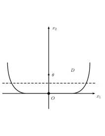
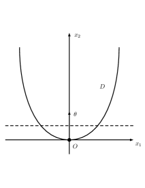
Figure 2. Regularity of $R\chi_{D}(s,\theta)$. We consider $\theta$ in the direction of $x_{2}$-axis. Then $R\chi_{D}(s,\theta)$ is the integration of $\chi_{D}(x)$ along the dashed line with distance $s$ to $x_{1}$-axis. Left figure: $D$ is not strictly convex near $O$. $R\chi_{D}(s,\theta)$ has a Heaviside type singularity in $s$. Right figure: $D$ is strictly convex near $O$. Then $R\chi_{D}(s,\theta)$ behaves like a homogeneous distribution $s_{+}^{1/2}$ in $s$.

Below, we use $t_{+}^{\alpha},\alpha>-1$ to denote homogeneous distributions so that $t_{+}^{\alpha}=t^{\alpha}$ for $t\geq 0$ and $t_{+}^{\alpha}=0$ for $t<0$. See Section 3.2 of [4] for details. The key result of this section is

Lemma 4.2.

Suppose $U$ is strictly convex. For $q_{0}\in S$, there exists a neighborhood of $q_{0}$ and local coordinates $y=(y_{1},y_{2})\in{\mathbb{R}}^{2}$ such that $q_{0}=(0,0)$, $S=\{y_{2}=0\}$ and

$$R\chi_{U}(y)=h(y)y_{2,+}^{1/2}+y_{2,+}r(y),\quad r\in I^{-3/2}(M;S)$$

where $h$ is smooth and positive.

Note that $y_{2,+}\in I^{-3/2}(M;S)$ so the product $y_{2,+}r(y)$ makes sense as product of distributions in $I^{-3/2}(M;S)$ by Lemma 3.1. Also, note that $I^{-3/2}(M;S)\subset L^{\infty}$, see [2] so the product also makes sense in $L^{\infty}.$

Proof.

Recall that $\partial U$ is a simple closed strictly convex curve if and only if the curvature $\kappa$ is strictly positive on $\partial U$, see Section 2.3 of [8]. Here, the curvature is defined in the Frenet frame and is always non-negative.

For any $q_{0}\in S$, we consider a neighborhood and local coordinates $(y_{1},y_{2})$ such that $q_{0}=(0,0)$ and $S$ is given by $y_{2}=0$. Then we write $s=s(y_{1},y_{2})$ and $\phi=\phi(y_{1},y_{2})$ as smooth functions. Consider the Radon transform

(14) $$\begin{gathered}R\chi_{D}(y_{1},y_{2})=\frac{1}{2\pi}\int_{{\mathbb{R}}^{2}}\int_{{\mathbb{R}}}e^{i\lambda(s-x_{1}\cos\phi-x_{2}\sin\phi)}\chi_{D}(x)d\lambda dx_{1}dx_{2}.\end{gathered}$$

For any $\phi$, we let $q$ be a point on $\partial U$ such that $\theta=(\cos\phi,\sin\phi)$ is orthogonal to $T_{q}(\partial U)$. (By the strict convexity of $U$, there are two points with this property.) We compute the integral in (14) in the Frenet frame at $p$. Thus, we choose local coordinates $(z_{1},z_{2})$ near $p$ such that $q=(0,0)$ and $z_{1}$ axis is tangent to $\partial U$ at $q$. Moreover, by selecting the orientation of $\partial U$, we can arrange the new coordinate system to have the same orientation as the original one and $U$ stays in $z_{2}>0.$ Let $\Phi:{\mathbb{R}}^{2}\rightarrow{\mathbb{R}}^{2}$ be the coordinate change so $z=\Phi(x;y)$. Note $\Phi$ depends on $y$ and is smooth in $y.$ Then we write $dx=J(z;y)dz$ where $J$ is the Jacobian factor and $J>0.$ Note that in this new coordinate system, we have $x_{1}\cos\phi+x_{2}\sin\phi=s_{0}\pm z_{2}$ where the sign is $+$ if $\theta$ is in the direction of positive $z_{2}$ axis and $-$ otherwise.

Suppose $\partial U$ is parameterized by arc-length $\tau$ starting from $q$. Then in the Frenet frame, we have the canonical form of the curve

$$z_{1}(\tau)=\tau-\frac{\kappa^{2}\tau^{3}}{6}+o(\tau^{3}),\quad z_{2}(\tau)=\frac{\kappa}{2}\tau^{2}+\frac{\kappa^{\prime}\tau^{3}}{6}+o(\tau^{3})$$

see Section 1-6 of [1]. Here, $\kappa,\kappa^{\prime}$ are the curvature and its $\tau$ derivative at $q.$ As $\kappa>0,$ by using the inverse function theorem, we can take $z_{1}\in(-\delta,\delta)$ with $\delta>0$ small as the parameter and express the curve as the graph of a function

$$z_{2}=\frac{\kappa}{2}z_{1}^{2}+\frac{\kappa^{\prime}z_{1}^{3}}{6}+o(z_{1}^{3})$$

For $z_{1}\geq 0$, the function is invertible and we have

$$z_{1}=(\frac{2}{\kappa})^{\frac{1}{2}}z_{2}^{\frac{1}{2}}+a_{3}z_{2}^{\frac{3}{2}}+\cdots,\quad z_{2}\geq 0.$$

Finally, we go back to (14) and get

$$\begin{split}R\chi_{D}(y)&=\frac{1}{2\pi}\int_{{\mathbb{R}}}e^{i\lambda(s-s_{0}\pm z_{2})}\int_{{\mathbb{R}}^{2}}\chi_{D}(z)J(z;y)dzd\lambda\\ &=\int_{{\mathbb{R}}}e^{i\lambda(s-s_{0}\pm z_{2})}(\int_{0}^{\delta}(a_{1}(y,z_{2})z_{2}^{\frac{1}{2}}+a_{3}(y,z_{2})z_{2}^{\frac{3}{2}}+\cdots)dz_{2})d\lambda\\ &=c_{1}(y)(s-s_{0})^{\frac{1}{2}}_{+}+c_{2}(y)(s-s_{0})^{\frac{3}{2}}_{+}+\cdots\end{split}$$

For the second line, we used Taylor expansion of $J(z;y)$ in $z_{1}.$ Note that $a_{1}>0$. For the last line, we used the Taylor expansion of $a_{n},n=1,2,\cdots$ in $z_{2}$ and integrated in $z_{2}.$ Note that $c_{1}(y)>0.$ This completes the proof of the lemma. ∎

Next, we consider the situation near $S_{\diamond}$.

Lemma 4.3.

Suppose $D_{1},D_{2}$ are strictly convex. For $q_{0}\in S_{1}\cap S_{2}$, there is local coordinates $y=(y_{1},y_{2})\in{\mathbb{R}}^{2}$ near $q_{0}$ such that locally $q_{0}=(0,0),$ $S_{1}=\{y_{2}=0\},S_{2}=\{y_{1}=0\}$ and

$$\begin{gathered}R\chi_{D_{1}}(y)=h_{1}(y)y_{2,+}^{1/2}+y_{2,+}r_{1}(y),\quad r_{1}\in I^{-3/2}(M;S_{1})\\ R\chi_{D_{2}}(y)=h_{2}(y)y_{1,+}^{1/2}+y_{1,+}r_{2}(y),\quad r_{2}\in I^{-3/2}(M;S_{2})\end{gathered}$$

where $h_{j},j=1,2$ are smooth and positive.

Proof.

First, we apply Lemma 4.3 to find a neighborhood $V_{1}$ of $q_{0}$ and coordinates $(z_{1},z_{2})$ such that $S_{1}=\{z_{2}=0\}$. Then we apply Lemma 4.3 again to find a neighborhood $V_{2}$ of $q_{0}$ and coordinates $(w_{1},w_{2})$ such that $S_{2}=\{w_{2}=0\}$. Because $S_{1}$ intersects $S_{2}$ transversally at $q_{0}$ see [10], we know that the $z_{2}$ axis is not parallel to $w_{2}$ axis. Thus, we can find a new coordinate system $(y_{1},y_{2})$ with $y_{1}=z_{2},y_{2}=w_{2}$. Then we write $z_{1}=z_{1}(y),w_{1}=w_{1}(y)$ as smooth functions. Finally, the conclusions follows from Lemma 4.3. ∎

The vanishing order is the key for obtaining multiplicative properties similar to Piriou’s distributions.

Lemma 4.4.

Let $m,n\in{\mathbb{N}}.$ Under the assumptions of Lemma 4.3, we have

1. For $j=1,2$, $(R\chi_{D_{j}})^{n}(y)=h_{j}(y)y_{2,+}^{n/2}+y_{2,+}^{1+n/2}r_{j}(y),$ where $r_{j}\in I^{-3/2}(M;S_{j})$ and $h_{j}$ is smooth and positive.

2. $(R\chi_{D_{1}})^{m}(y)(R\chi_{D_{2}})^{n}(y)=h(y)y_{2,+}^{m/2}y_{1,+}^{n/2}+r(y)$, where $r$ is a sum of paired Lagrangian distributions such that $r\in I^{-5/2-m/2-n/2}(T_{q_{0}}^{*}M\backslash(N^{*}S_{1}\cup N^{*}S_{2}))$.

Proof.

(1). We prove for $n=2$. The general case can be obtained by induction. We can find a proper coordinates as in Lemma 4.2 and write for $j=1,2$

$$R\chi_{D_{j}}(y)=\tilde{h}(y)y_{2,+}^{1/2}+y_{2,+}\tilde{r}(y),\quad\tilde{r}\in I^{-3/2}(M;S_{j})$$

Then

$$(R\chi_{D_{j}})^{2}=\tilde{h}^{2}(y)y_{2,+}+2\tilde{h}(y)\tilde{r}(y)y_{2,+}^{3/2}+y_{2,+}^{2}\tilde{r}^{2}(y)$$

Note that $\tilde{h}\tilde{r}\in I^{-3/2}(M;S_{j})$. Also, $\tilde{r}^{2}\in I^{-3/2}(M;S_{j})$ so $y_{2,+}^{\frac{1}{2}}\tilde{r}^{2}\in I^{-3/2}(M;S_{j})$ as well.

(2). We use the coordinates in Lemma 4.3 to get

$$\begin{gathered}(R\chi_{D_{1}})^{m}(y)=h_{1}(y)y_{2,+}^{m/2}+y_{2,+}^{1+m/2}r_{1}(y),\quad r_{1}\in I^{-3/2}(M;S_{1})\\ (R\chi_{D_{2}})^{n}(y)=h_{2}(y)y_{1,+}^{n/2}+y_{1,+}^{1+n/2}r_{2}(y),\quad r_{2}\in I^{-3/2}(M;S_{2})\end{gathered}$$

where $h_{1},h_{2}$ are smooth and positive functions. Thus

$$\begin{gathered}(R\chi_{D_{1}})^{m}(y)(R\chi_{D_{2}})^{n}(y)=h_{1}(y)h_{2}(y)y_{2,+}^{m/2}y_{1,+}^{n/2}+h_{1}(y)r_{2}(y)y_{2,+}^{m/2}y_{1,+}^{1+n/2}\\ +h_{2}(y)r_{1}(y)y_{1,+}^{n/2}y_{2,+}^{1+m/2}+y_{2,+}^{m/2+1}y_{1,+}^{n/2+1}r_{1}(y)r_{2}(y).\end{gathered}$$

Note that $h_{1}r_{2}\in I^{-3/2}(M;S_{2})$. Then by using Proposition 2.4 of [16], we see that $h_{1}(y)r_{2}(y)y_{2,+}^{m/2}\in I^{-1-m/2}(M;S_{2})$. By using the proof of Lemma 12 (here, we need the result for different orders but the proof is the same, see also [2]), we get

(15) $$\begin{gathered}h_{1}(y)r_{2}(y)y_{2,+}^{m/2}y_{1,+}^{1+n/2}\in I^{-1-m/2,-3/2-n/2}(T^{*}_{q_{0}}M,N^{*}S_{2})\\ +I^{-2-n/2,-1/2-m/2}(T^{*}_{q_{0}}M,N^{*}S_{1}).\end{gathered}$$

Similarly, we obtain that

(16) $$\begin{gathered}h_{2}(y)r_{1}(y)y_{1,+}^{n/2}y_{2,+}^{1+m/2}\in I^{-1-n/2,-3/2-m/2}(T^{*}_{q_{0}}M,N^{*}S_{1})\\ +I^{-2-m/2,-1/2-n/2}(T^{*}_{q_{0}}M,N^{*}S_{2}),\\ y_{2,+}^{m/2+1}y_{1,+}^{n/2+1}r_{1}(y)r_{2}(y)\in I^{-2-n/2,-3/2-m/2}(T^{*}_{q_{0}}M,N^{*}S_{1})\\ +I^{-2-m/2,-3/2-n/2}(T^{*}_{q_{0}}M,N^{*}S_{2}).\end{gathered}$$

We conclude that away from $N^{*}S_{1}\cup N^{*}S_{2}$, terms in (15) and (16) belong to $I^{-5/2-m/2-n/2}(T_{q_{0}}^{*}M)$. This completes the proof. ∎

5. Determination of the nonlinear term

Proof of Theorem 2.1.

Suppose $\tilde{F}(t)=\sum_{j=2}^{\tilde{J}}\tilde{a}_{j}t^{j}$ is another nonlinear polynomial of the form (4). Let $\tilde{P}_{MA},\tilde{f}_{CT}$ be the corresponding functions for $\tilde{F}$. Assume that $f_{CT}=\tilde{f}_{CT}$. We consider

(17) $$P_{MA}-\tilde{P}_{MA}=\sum_{j=2}^{J}(a_{j}-\tilde{a}_{j})(R\chi_{D})^{j}.$$

Here, we assumed $J\geq\tilde{J}$ and we let $\tilde{a}_{j}=0$ for $j>\tilde{J}.$ We claim that for any $q\in S_{\diamond}$,

(18) $$\text{WF}(P_{MA}-\tilde{P}_{MA})\cap(T^{*}_{q}M\backslash(N^{*}S_{1}\cup N^{*}S_{2}))=\emptyset.$$

To see this, we first use Lemma 4.4 to conclude that $P_{MA}-\tilde{P}_{MA}$ is a sum of Lagrangian distributions and paired Lagrangian distributions exactly as those in the proof of Lemma 3.3 but with different orders. Then the symbol calculation in Lemma 3.3 yields the claim because $f_{CT}-\tilde{f}_{CT}$ is smooth away from $\partial D.$

Next, we show that $a_{j}=\tilde{a}_{j}$ in (17). Without loss of generality, we can take $\tilde{a}_{j}=0$ and show $a_{j}=0.$ We expand and regroup the terms in (17) as following

$$\begin{gathered}\sum_{j=2}^{J}a_{j}(R\chi_{D})^{j}=\sum_{j=2}^{J}a_{j}(R\chi_{D_{1}})^{j}+\sum_{j=2}^{J}a_{j}(R\chi_{D_{2}})^{j}+\sum_{j=2}^{J}a_{j}A_{j}\\ \text{ where }A_{j}=\sum_{m+n=j,m,n\geq 1}C_{m,n}(R\chi_{D_{1}})^{m}(R\chi_{D_{2}})^{n},\quad C_{m,n}>0.\end{gathered}$$

To determine $a_{j},$ we use singularities at $T_{q}^{*}M$ for $q\in S_{\diamond}$ away from $N^{*}S_{1}\cup N^{*}S_{2}$ so it suffices to look at singularities in $A_{j}.$ According to Lemma 4.4, we know that

$$A_{j}=\sum_{m+n=j,m,n\geq 1}C_{m,n}h_{m,n}(y)y_{2,+}^{m/2}y_{1,+}^{n/2}+r_{m,n}(y),$$

where $C_{m,n}$ and $h_{m,n}$ are both positive. Note that microlocally in $T_{q}^{*}M\backslash(N^{*}S_{1}\cup N^{*}S_{2}),$ we have $C_{m,n}h_{m,n}(y)y_{2,+}^{m/2}y_{1,+}^{n/2}\in I^{-2-m/2-n/2}(T_{q}^{*}M)$. We know from Lemma 4.4 that $r_{m,n}\in I^{-5/2-m/2-n/2}(T_{q}^{*}M).$ Thus microlocally, $A_{j}\in I^{-2-j/2}(T_{q}^{*}M)$. To see that the principal symbol is non-vanishing, it suffices to find the Fourier transform of $A_{j,0}=\sum_{m+n=j,m,n\geq 1}C_{m,n}h_{m,n}(0)y_{2,+}^{m/2}y_{1,+}^{n/2}$. Recall from Example 7.1.17 and Section 3.2 of [4] that the Fourier transform of $x_{+}^{a},\operatorname{Re}a>-1$ is $\Gamma(a+1)e^{i\pi(a+1)/2}(\xi-i0)^{-a-1}$. Thus, the Fourier transform of $A_{j,0},j\geq 2$ is given by

$$\sum_{m+n=j,m,n\geq 1}C_{m,n}h_{m,n}(0)\Gamma(\frac{m}{2}+1)\Gamma(\frac{n}{2}+1)e^{i\pi(j/2+1)/2}(\xi_{1}-i0)^{-m/2-1}(\xi_{2}-i0)^{-n/2-1}$$

Note that $C_{m,n},h_{m,n}(0)$ and the Gamma function terms are all positive. The exponential factor is the same for all terms in the summation. Thus, the principal symbol of $A_{j}$ on $T_{q}^{*}M\backslash(N^{*}S_{1}\cup N^{*}S_{2})$ is non-vanishing.

Now we can finish the proof. For $j=2$, we get that microlocally in $T_{q}^{*}M\backslash(N^{*}S_{1}\cup N^{*}S_{2})$, $A_{2}\in I^{-5/2}(T_{q}^{*}M)$ and $A_{j}\in I^{-7/2}(T_{q}^{*}M)$ for $j\geq 3$. Because the principal symbol of $A_{2}$ is non-vanishing, we derive from the claim in the beginning of the proof that $a_{2}=0$. Now we can repeat the argument for $j=3,\cdots,J$ to get that all $a_{j}=0$. This finishes the proof. ∎

Proof of Corollary 2.2.

If $F=0$, it is easy to see from (6) that $f_{CT}\in C^{\infty}({\mathbb{R}}^{2}\backslash\partial D).$ If $f_{CT}\in C^{\infty}$ away from $\partial D$, we know from the proof of Theorem 2.1 that (18) holds true for $\tilde{P}_{MA}=0$ and $\tilde{a}_{j}=0,j=1,2,\cdots,J$. Then the proof of Theorem 2.1 implies that $F=0.$ ∎

6. Acknowledgments

The author wishes to thank Prof. Jin Keun Seo for helpful conversations about the nonlinear nature of the beam-hardening artifacts. This work is supported by NSF under grant DMS-2205266.

Appendix A Composition of FIOs

In this appendix, we verify some technical conditions for the composition of Fourier integral operators in Section 3. We recall some definitions from [6, Section 25.2]. Let $X,Y,Z$ be three manifolds. Let $C_{1}$ be a homogeneous canonical relation from $T^{*}Y\backslash 0$ to $T^{*}X\backslash 0$ and $C_{2}$ be a homogeneous canonical relation from $T^{*}Z\backslash 0$ to $T^{*}Y\backslash 0$, we say that the composition $C_{2}\circ C_{1}$ is transversal if ${\mathscr{X}}=C_{1}\times C_{2}$ intersects ${\mathscr{Y}}=T^{*}X\times\Delta(T^{*}Y)\times T^{*}Z$ transversally, that is for any $q$ in the intersection

$$T_{q}{\mathscr{X}}+T_{q}{\mathscr{Y}}=T_{q}{\mathscr{Z}}\text{ with }{\mathscr{Z}}=T^{*}X\times T^{*}Y\times T^{*}Y\times T^{*}Z$$

Here, $\Delta(T^{*}Y)$ denotes the diagonal set of $T^{*}Y\times T^{*}Y.$ The composition is proper if the map ${\mathscr{X}}\cap{\mathscr{Y}}\rightarrow T^{*}(X\times Z)\backslash 0$ is proper. If the composition is transversal and proper, then $C=C_{2}\circ C_{1}$ is a canonical relation. We have Theorem 25.2.3 of [6] for the composition of FIOs. Actually, we only need the special case of transversal compositions. For the study of composition of Fourier integral operators and conormal distributions, we take $Z$ to be a point, see the treatment on page 22 of [6].

We start with the composition of $C$ and $C_{j},j=1,2$ in Section 3.1. Recall from (8) that the canonical relation of $R$ is parametrized as

$$\begin{gathered}C=\{(x_{1}\cos\phi+x_{2}\sin\phi,\phi,-\lambda,\lambda(-x_{1}\sin\phi+x_{2}\cos\phi);\\ x_{1},x_{2},-\lambda\cos\phi,-\lambda\sin\phi):\\ \lambda\in{\mathbb{R}}\backslash 0,\phi\in(-\pi,\pi),x_{1},x_{2}\in{\mathbb{R}}\}\subset T^{*}M\backslash 0\times T^{*}{\mathbb{R}}^{2}\backslash 0\end{gathered}$$

For $C_{j}=N^{*}\partial D_{j}\backslash 0,j=1,2$, we choose local coordinates $(y_{1},y_{2})$ near $q\in\partial D_{j}$ such that $q=0$ and $D_{j}=\{y_{2}=0\}.$ Then $C_{j}=\{(y_{1},0,0,\xi_{2}):y_{1}\in{\mathbb{R}},\xi_{2}\in{\mathbb{R}}\backslash 0\}.$ Now we let ${\mathscr{Z}}=T^{*}M\times T^{*}{\mathbb{R}}^{2}\times T^{*}{\mathbb{R}}^{2},{\mathscr{X}}=C\times C_{j}\subset{\mathscr{Z}}$ and ${\mathscr{Y}}=T^{*}M\times\Delta(T^{*}{\mathbb{R}}^{2})\subset{\mathscr{Z}}$. Note that ${\mathscr{X}}$ is parametrized by $x_{1},x_{2},\lambda,\phi,y_{1},\xi_{2}\in{\mathbb{R}}$ and we write an element of ${\mathscr{Y}}$ as $(s,\psi,\alpha,\beta;z_{1},z_{2},\eta_{1},\eta_{2},$ $z_{1},z_{2},\eta_{1},\eta_{2})$ with all variables in ${\mathbb{R}}.$ The intersection ${\mathscr{X}}\cap{\mathscr{Y}}$ is given by

$$\begin{gathered}s=x_{1}\cos\phi+x_{2}\sin\phi,\psi=\phi,\alpha=-\lambda,\beta=\lambda(-x_{1}\sin\phi+x_{2}\cos\phi),\\ x_{1}=y_{1}=z_{1},x_{2}=y_{2}=z_{2}=0,-\lambda\cos\phi=0=\eta_{1},-\lambda\sin\phi=\xi_{2}=\eta_{2}\end{gathered}$$

which implies that $\phi=\pm\pi/2$ so

$$\begin{gathered}{\mathscr{X}}\cap{\mathscr{Y}}=\{(0,\pm\pi/2,-\lambda,\mp\lambda x_{1};x_{1},0,0,\mp\lambda,x_{1},0,0,\mp\lambda):x_{1},\lambda\in{\mathbb{R}}\}.\end{gathered}$$

We see that the projection to $T^{*}M$ is proper. Let $q\in{\mathscr{X}}\cap{\mathscr{Y}}$. To compute the tangent vector of $T_{q}{\mathscr{X}}$, we use the map $\pi:{\mathbb{R}}^{6}_{(x_{1},x_{2},\lambda,\phi,y_{1},\xi_{2})}\rightarrow{\mathscr{X}}$. So a general tangent vector at $q$ can be obtained by

$$\begin{gathered}\pi_{*}(\delta x_{1},\delta x_{2},\delta\lambda,\delta\phi,\delta y_{1},\delta\xi_{2})\\ =(\delta x_{2}-x_{1}\delta\phi,\delta\phi,-\delta\lambda,-\lambda\delta x_{1}-x_{1}\delta\lambda,\delta x_{1},\delta x_{2},\lambda\delta\phi,-\delta\lambda,\delta y_{1},0,0,\delta\xi_{2})\end{gathered}$$

For the tangent vector of $T_{q}{\mathscr{Y}}$, we use the map $\rho:{\mathbb{R}}^{8}_{(s,\psi,\alpha,\beta;z_{1},z_{2},\eta_{1},\eta_{2})}\rightarrow{\mathscr{Y}}$ to get

$$\begin{gathered}\rho_{*}(\delta s,\delta\psi,\delta\alpha,\delta\beta;\delta z_{1},\delta z_{2},\delta\eta_{1},\delta\eta_{2})\\ =(\delta s,\delta\psi,\delta\alpha,\delta\beta;\delta z_{1},\delta z_{2},\delta\eta_{1},\delta\eta_{2},\delta z_{1},\delta z_{2},\delta\eta_{1},\delta\eta_{2})\end{gathered}$$

Now we conclude that $T_{q}{\mathscr{X}}+T_{q}{\mathscr{Y}}=T_{q}{\mathscr{Z}}$ by listing $12$ linearly independent tangent vectors which is quite straightforward.

Next, consider the composition of $C^{*}$ and $C_{0}=T_{q}^{*}M\backslash 0$ needed in Lemma 3.3. From (8), we get

(19) $$\begin{gathered}C^{*}=\{(x_{1},x_{2},-\lambda\cos\phi,-\lambda\sin\phi;x_{1}\cos\phi+x_{2}\sin\phi,\phi,\\ -\lambda,\lambda(-x_{1}\sin\phi+x_{2}\cos\phi)):\lambda\in{\mathbb{R}}\backslash 0,\phi\in(-\pi,\pi),x_{1},x_{2}\in{\mathbb{R}}\}\end{gathered}$$

We write

$$C_{0}=\{(0,0,\zeta_{1},\zeta_{2}):\zeta_{1},\zeta_{2}\in{\mathbb{R}},\zeta_{1}\zeta_{2}\neq 0\}$$

Then let ${\mathscr{X}}=C^{*}\times C_{0}$, ${\mathscr{Y}}=T^{*}{\mathbb{R}}^{2}\times\Delta(T^{*}M)$ and ${\mathscr{Z}}=T^{*}{\mathbb{R}}^{2}\times T^{*}M\times T^{*}M.$ The intersection ${\mathscr{X}}\cap{\mathscr{Y}}$ is given by

$$x_{1}\cos\phi+x_{2}\sin\phi=0,\phi=0,-\lambda=\zeta_{1},\lambda(-x_{1}\sin\phi+x_{2}\cos\phi)=\zeta_{2}$$

which implies $x_{1}=0,\phi=0$ so

$${\mathscr{X}}\cap{\mathscr{Y}}=\{(0,x_{2},-\lambda,0;0,0,-\lambda,-\lambda x_{2}):\lambda,x_{2}\in{\mathbb{R}}\}$$

The projection to $T^{*}{\mathbb{R}}^{2}$ is proper. Let $q\in{\mathscr{X}}\cap{\mathscr{Y}}$. To compute the tangent vector of $T_{q}{\mathscr{X}}$, we use the map $\pi:{\mathbb{R}}^{6}_{(x_{1},x_{2},\lambda,\phi,\alpha,\beta)}\rightarrow{\mathscr{X}}$. So

$$\begin{gathered}\pi_{*}(\delta x_{1},\delta x_{2},\delta\lambda,\delta\phi,\delta\zeta_{1},\delta\zeta_{2})\\ =(\delta x_{1},\delta x_{2},-\delta\lambda,-\lambda\delta\phi,\delta x_{1}+x_{2}\delta\phi,\delta\phi,-\delta\lambda,x_{2}\delta\lambda,\lambda\delta x_{2},0,0,\delta\zeta_{1},\delta\zeta_{2})\end{gathered}$$

For the tangent vector of $T_{q}{\mathscr{Y}}$, we use $(z_{1},z_{2},\eta_{1},\eta_{2};s,\phi,\alpha,\beta;s,\phi,\alpha,\beta)$ for a general element of ${\mathscr{Y}}$. Consider $\rho:{\mathbb{R}}^{8}_{(z_{1},z_{2},\eta_{1},\eta_{2};s,\phi,\alpha,\beta)}\rightarrow{\mathscr{Y}}$ and we get

$$\begin{gathered}\rho_{*}(\delta z_{1},\delta z_{2},\delta\eta_{1},\delta\eta_{2};\delta s,\delta\psi,\delta\alpha,\delta\beta)\\ =(\delta z_{1},\delta z_{2},\delta\eta_{1},\delta\eta_{2},\delta s,\delta\psi,\delta\alpha,\delta\beta,\delta s,\delta\psi,\delta\alpha,\delta\beta)\end{gathered}$$

We can also see that $T_{q}{\mathscr{X}}+T_{q}{\mathscr{Y}}=T_{q}{\mathscr{Z}}$.

Finally, we consider the composition of $C^{*}$ and $\tilde{C}_{j}=N^{*}S_{j}\backslash 0,j=1,2$ needed in Lemma 3.3. In this case, we can find local coordinates $(y_{1},y_{2})$ near $p\in S_{j}$ so that $p=0$ and $S_{j}=\{y_{1}=0\}$. Thus,

$$\tilde{C}_{j}=\{(0,y_{2},\eta_{1},0):y_{2}\in{\mathbb{R}},\eta_{1}\in{\mathbb{R}}\backslash 0\}$$

Then let ${\mathscr{X}}=C^{*}\times\tilde{C}_{j}$, ${\mathscr{Y}}=T^{*}{\mathbb{R}}^{2}\times\Delta(T^{*}M)$ and ${\mathscr{Z}}=T^{*}{\mathbb{R}}^{2}\times T^{*}M\times T^{*}M.$ Using (19), the intersection ${\mathscr{X}}\cap{\mathscr{Y}}$ is given by

$$x_{1}\cos\phi+x_{2}\sin\phi=0,\phi=y_{2},-\lambda=\eta_{1},\lambda(-x_{1}\sin\phi+x_{2}\cos\phi)=0$$

which implies $x_{1}=x_{2}=0$ so

$${\mathscr{X}}\cap{\mathscr{Y}}=\{(0,0,-\lambda\cos\phi,-\lambda\sin\phi,0,\phi,-\lambda,0,0,\phi,-\lambda,0):\lambda,\phi\in{\mathbb{R}}\}$$

The projection to $T^{*}{\mathbb{R}}^{2}$ is proper. To compute the tangent vector of $T_{q}{\mathscr{X}}$, we use the map $\pi:{\mathbb{R}}^{6}_{(x_{1},x_{2},\lambda,\phi,y_{2},\eta_{1})}\rightarrow{\mathscr{X}}$. So

$$\begin{gathered}\pi_{*}(\delta x_{1},\delta x_{2},\delta\lambda,\delta\phi,\delta\zeta_{1},\delta\zeta_{2})\\ =(\delta x_{1},\delta x_{2},-\delta\lambda\cos\phi+\lambda\sin\phi d\phi,-\delta\lambda\sin\phi-\lambda\cos\phi\delta\phi;\\ \delta x_{1}\cos\phi+\delta x_{2}\sin\phi,\delta\phi,-\delta\lambda,-\lambda\delta x_{1}\sin\phi+\lambda\delta x_{2}\cos\phi,0,\delta y_{2},-\delta\lambda,0)\end{gathered}$$

For the tangent vector of $T_{q}{\mathscr{Y}}$, we use $(z_{1},z_{2},\eta_{1},\eta_{2};s,\phi,\alpha,\beta;s,\phi,\alpha,\beta)$ for a general element of ${\mathscr{Y}}$. Let $\rho:{\mathbb{R}}^{8}_{(z_{1},z_{2},\eta_{1},\eta_{2};s,\phi,\alpha,\beta)}\rightarrow{\mathscr{Y}}$ to get

$$\begin{gathered}\rho_{*}(\delta z_{1},\delta z_{2},\delta\eta_{1},\delta\eta_{2};\delta s,\delta\psi,\delta\alpha,\delta\beta)\\ =(\delta z_{1},\delta z_{2},\delta\eta_{1},\delta\eta_{2},\delta s,\delta\psi,\delta\alpha,\delta\beta,\delta s,\delta\psi,\delta\alpha,\delta\beta)\end{gathered}$$

Again, we can find 12 linearly independent vectors to see that $T_{q}{\mathscr{X}}+T_{q}{\mathscr{Y}}=T_{q}{\mathscr{Z}}$.

References

- [1] M. P. do Carmo, Differential Geometry of Curves and Surfaces: Revised and Updated Second Edition. Courier Dover Publications, 2016.
- [2] A. Greenleaf, G. Uhlmann. Recovering singularities of a potential from singularities of scattering data. Communications in Mathematical Physics 157.3 (1993): 549-572.
- [3] V. Guillemin, G. Uhlmann. Oscillatory integrals with singular symbols. Duke Math. J 48.1 (1981): 251-267.
- [4] L. Hörmander. The Analysis of Linear Partial Differential Operators I: Distribution theory and Fourier analysis. Second edition. Springer-Verlag, 1989.
- [5] L. Hörmander. The Analysis of Linear Partial Differential Operators III: Pseudo-Differential Operators. Classics in Mathematics (2007).
- [6] L. Hörmander. The Analysis of Linear Partial Differential Operators IV: Fourier Integral Operators. Classics in Mathematics (2009).
- [7] A. Katsevich. Local tomography with nonsmooth attenuation. Transactions of the American Mathematical Society 351.5 (1999): 1947-1974.
- [8] W. Klingenberg. A Course in Differential Geometry. Vol. 51. Springer Science & Business Media, 2013.
- [9] Y. Kurylev, M. Lassas and G. Uhlmann. Inverse problems for Lorentzian manifolds and non-linear hyperbolic equations. Inventiones Mathematicae 212.3 (2018): 781-857.
- [10] B. Palacios, G. Uhlmann, Y. Wang. Quantitative analysis of metal artifacts in X-ray tomography. SIAM Journal on Mathematical Analysis 50.5 (2018): 4914-4936.
- [11] H. S. Park, J. K. Choi, J. K. Seo. Characterization of metal artifacts in X-ray computed tomography. Communications on Pure and Applied Mathematics 70.11 (2017): 2191-2217.
- [12] H. S. Park, D. Hwang, J. K. Seo. Metal artifact reduction for polychromatic X-ray CT based on a beam-hardening corrector. IEEE Transactions on Medical Imaging 35.2 (2015): 480-487.
- [13] H. S. Park, S. M. Lee, H. P. Kim, J. K. Seo. Machine-learning-based nonlinear decomposition of CT images for metal artifact reduction. arXiv:1708.00244 (2017).
- [14] A. Piriou. Calcul symbolique non linéaire pour une onde conormale simple. Annales de l’institut Fourier. Vol. 38. No. 4. 1988.
- [15] T. E. Quinto. An introduction to X-ray tomography and Radon transforms. Proceedings of Symposia in Applied Mathematics. Vol. 63. 2006.
- [16] A. Sá Barreto, Y. Wang. Singularities generated in the triple interaction of semilinear conormal waves. Analysis & PDE 14.1 (2021): 135-170.
- [17] Y. Wang, Y. Zou. Streak artifacts from non-convex metal objects in X-ray tomography. Pure and Applied Analysis. 3.2 (2021): 295-318.
- [18] Y. Zhang, H. Yu. Convolutional neural network based metal artifact reduction in X-ray computed tomography. IEEE Transactions on Medical Imaging 37.6 (2018): 1370-1381.