Coordination for Connected Automated Vehicles at Merging Roadways in Mixed Traffic Environment

Abstract

In this paper, we present an optimal control framework to address motion coordination of connected automated vehicles (CAVs) in the presence of human-driven vehicles (HDVs) in merging scenarios. Our framework combines an unconstrained trajectory solution of a low-level energy-optimal control problem with an upper-level optimization problem that yields the minimum travel time for CAVs. We predict the future trajectories of the HDVs using Newell’s car-following model. To handle potential deviations of HDVs’ actual behavior from the predicted one, we design a safety filter for CAVs based on control barrier functions. The effectiveness of the proposed control framework is demonstrated via simulations with heterogeneous human driving behaviors.

I Introduction

Emerging vehicular technologies in automation and communication have generated new opportunities to enhance traffic safety and efficiency [1]. Prior research efforts have shown that in environments consisting solely of connected automated vehicles (CAVs), the traffic throughput and energy consumption can be significantly improved under different vehicle coordination strategies such as optimal control [2, 3, 4], model predictive control [5], control barrier functions [6], and learning-based control [7, 8]. It is expected that CAVs will gradually penetrate the market and interact with human-driven vehicles (HDVs) over the next several years. The presence of HDVs, however, complicates vehicle coordination, given the existing limitations on predicting precise driving behavior [9].

Addressing coordination of CAVs in a mixed traffic environment, where CAVs and HDVs co-exist, has attracted considerable attention recently. Some examples include game theory combined with reinforcement learning [10], dynamic programming [11], statistical modeling of human uncertainties [12], and reachability analysis [13, 14]. Efforts on experimental validation with scaled robotic cars have been reported in [15]. In mixed autonomy, traffic bottlenecks such as merging roadways and intersections pose significant challenges to the decision-making and control of CAVs. A centralized algorithm for socially compliant navigation at an intersection given the social preferences of the vehicles was presented in [16]. A hierarchical on-ramp merging control strategy for CAVs was presented in [17], where an upper-level planner computes an expected merging position and a low-level trajectory controller guarantees constraints under uncertainties of HDVs. A vehicle coordination problem for a signal-free intersection using vehicle platooning was addressed in [18].

In this paper, we extend the framework developed in [2, 4] for CAV coordination to a mixed-traffic merging scenario. We present an optimal control formulation to derive the trajectories for the CAVs, in which the unconstrained trajectory solution of a low-level energy-optimal control problem is embedded in an upper-level optimization problem aimed at finding the minimum travel time for the CAV. We employ Newell’s car-following model [19] to predict the HDVs’ future trajectories, which are used to formulate no-conflict constraints in the optimal control problem. The constraints help each CAV avoid conflicts with the vehicles traveling on the same road and those traveling on the other merging road. Since the predicted trajectories may deviate from those arising from the human drivers’ actions, we design a safety filter for the CAVs based on control barrier functions [20, 21]. The safety filter modifies the original optimal control input of the CAV in a minimally invasive fashion so that conflict-free maneuvers are ensured. We demonstrate the efficacy of the proposed framework by simulations given different levels of CAV penetration and traffic volumes.

The remainder of the paper proceeds as follows. In Section II, we formulate the coordination problem of CAVs in a mixed-traffic merging scenario. In Section III, we present the optimal control problem formulation combined with a method for predicting the future trajectories of HDVs, and a control barrier function-based safety filter. The simulation results are provided in Section IV. Finally, we draw concluding remarks in Section V.

II Problem Formulation

We consider the problem of coordinating multiple CAVs, co-existing with HDVs, in a scenario where two merging roadways intersect at a conflict point; see Fig. 1. We define a control zone inside which a coordinator is able to monitor the motion of all vehicles (including CAVs and HDVs). Communication errors or delays are neglected. The analysis of such effects is left for future research. Next, we provide the following necessary definitions for our exposition.

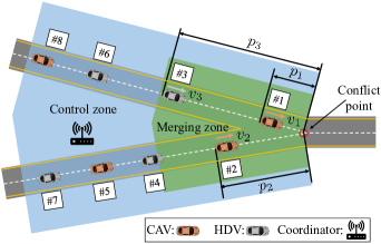
Figure 1: Merging scenario with two merging roadways intersecting at a conflict point. The blue area represents the control zone. In the merging zone (green area), virtual projection is utilized as detailed in Section III-B.

Definition 1

Let ${\mathcal{L}(t)=\{1,\ldots,L(t)\}}$, ${t\in\mathbb{R}_{\geq 0}}$, be the set of vehicles traveling inside the control zone at time $t$, where ${{L}(t)\in\mathbb{N}}$ is the total number of vehicles. Let ${\mathcal{A}(t)\subset\mathcal{L}(t)}$ and ${\mathcal{H}(t)\subset\mathcal{L}(t)}$ be the sets of CAVs and HDVs, respectively. For example, considering the scenario in Fig. 1, ${\mathcal{L}(t)=\{1,\dots,8\}}$, ${\mathcal{A}(t)=\{1,2,5,8\}}$, and ${\mathcal{H}(t)=\{3,4,6,7\}}$. Note that the indices of the vehicles are determined by the order in which they enter the control zone.

Definition 2

For a vehicle ${i\in\mathcal{L}(t)}$, let ${\mathcal{S}_{i}(t)\subset\mathcal{L}(t)}$ and ${\mathcal{N}_{i}(t)\subset\mathcal{L}(t)}$, ${t\in\mathbb{R}_{\geq 0}}$, be the sets of vehicles inside the control zone traveling on the same road as vehicle $i$ and on the neighboring road, respectively.

We consider that the dynamics of vehicle ${i\in\mathcal{L}(t)}$ are described by a double integrator model:

$$\begin{split}\dot{p}_{i}(t)&=v_{i}(t),\\ \dot{v}_{i}(t)&=u_{i}(t),\end{split}$$ (1)

where ${p_{i}\in\mathcal{P}}$, ${v_{i}\in\mathcal{V}}$, and ${u_{i}\in\mathcal{U}}$ denote the longitudinal position of the rear bumper, speed, and control input (acceleration) of the vehicle, respectively. The sets ${\mathcal{P},\mathcal{V},}$ and $\mathcal{U}$ are compact subsets of $\mathbb{R}$. Note that we set ${p_{i}=0}$ at the conflict point; see Fig. 1. The control input is bounded by

$$u_{\min}\leq u_{i}(t)\leq u_{\max},\quad\forall i\in\mathcal{L}(t),$$ (2)

where ${u_{\min}<0}$ and ${u_{\max}>0}$ are the minimum and maximum control inputs given by the physical acceleration and braking limits of the vehicles or imposed by driver/passenger comfort. Next, we provide the speed limits of the CAVs,

$$0\leq v_{i}(t)\leq v_{\max},\quad\forall i\in\mathcal{A}(t),$$ (3)

where ${v_{\max}>0}$ is the maximum allowable speed. We do not impose a maximum speed limit for HDVs since human drivers may violate it, but we still assume that

$$0\leq v_{i}(t),\quad\forall i\in\mathcal{H}(t),$$ (4)

which means the HDVs do not go backward.

To avoid conflicts between vehicles, we impose two types of constraints: (i) between vehicles traveling on neighboring roads (to avoid that they meet at the conflict point) and (ii) between vehicles traveling on the same road (to avoid rear-end collisions). To prevent a potential conflict between CAV–$i$ and a vehicle ${k\in\mathcal{N}_{i}(t)}$ traveling on the neighboring road, we require a minimum time gap ${t_{\min}>0}$ between the time instants ${t_{i}^{\mathrm{f}}}$ and $t_{k}^{\mathrm{f}}$ when the CAV–$i$ and vehicle $k$ cross the conflict point, respectively, i.e.,

$$\left\lvert t_{i}^{\mathrm{f}}-t_{k}^{\mathrm{f}}\right\rvert\geq t_{\min}.$$ (5)

To prevent rear-end collision between CAV–$i$ and its immediate preceding vehicle $k$ traveling on the same road, i.e., ${k=\max\,\{j\in\mathcal{S}_{i}(t)\;|\;j<i\}}$, we impose the constraint:

$$p_{k}(t)-p_{i}(t)\geq d_{\min}+t^{\mathrm{h}}_{\min}v_{i}(t),$$ (6)

where ${d_{\min}>0}$ and ${t^{\mathrm{h}}_{\min}>0}$ are the minimum standstill distance and the minimum time headway. Note that we use the distance between the vehicles’ rear bumpers, and the vehicle length is included by choosing sufficiently large ${d_{\min}}$.

III Optimal Control Formulation

In this section, we present an optimal control framework to coordinate the CAVs in mixed traffic, extending the one developed for 100% CAV penetration in [2, 4]. For each CAV, we use the unconstrained trajectory solution of a low-level energy-minimal optimal control problem to formulate an upper-level optimization problem that finds the minimum time for crossing the conflict point while satisfying all state, control, and safety constraints.

III-A Optimal Control Problems

We formulate the low-level optimization by considering that the solution to the upper-level optimization problem is known, i.e., that the minimum time $t_{i}^{\mathrm{f}}$ which satisfies all constraints is given. Then, the low-level optimal control problem aims at finding the control input (acceleration) for each CAV by solving the following optimization problem.

Problem 1: (Low-level energy-optimal control) Let $t_{i}^{0}$ and $t_{i}^{\mathrm{f}}$ be the times that CAV–$i$ enters and exits the control zone, respectively. Then, CAV–$i$ solves the following optimal control problem at $t_{i}^{0}$:

$$\begin{split}&\operatorname*{minimize}_{u_{i}(t)\in\mathcal{U}}\quad\frac{1}{2}\int_{t^{0}_{i}}^{t^{\mathrm{f}}_{i}}u^{2}_{i}(t)~{}\mathrm{d}t,\\ &\text{subject to:}\\ &\quad\eqref{eq:model2},\eqref{eq:uconstraint},\eqref{eq:vconstraint},\\ &\quad\eqref{eq:rearend_constraint},\;k=\max\,\{j\in\mathcal{S}_{i}(t_{i}^{0})\;|\;j<i\},\\ &\text{given:}\\ &\quad p_{i}(t_{i}^{0})=p^{0},\,\,v_{i}(t_{i}^{0})=v_{i}^{0},\,\,p_{i}(t_{i}^{\mathrm{f}})=0,\,\,u_{i}(t_{i}^{\mathrm{f}})=0,\end{split}$$ (7)

where $p^{0}$ is the position of the entry point of the control zone. The boundary conditions in (7) are set at the entry and exit of the control zone.

Note that (5) is not included in the low-level problem since the time $t_{i}^{\mathrm{f}}$, derived through the upper-level problem discussed below, satisfies (5). Also, note that in (7) we minimize the $L^{2}$ norm of control input $u_{i}(t)$ in ${t\in[t_{i}^{0},\ t_{i}^{\mathrm{f}}]}$ while the energy consumption per unit mass is given by

$$\varepsilon=\int_{t^{0}_{i}}^{t^{\mathrm{f}}_{i}}v_{i}(t)g(u_{i}(t))~{}\mathrm{d}t,$$ (8)

where ${g(x)=\max\{0,x\}}$. However, it was shown in [22] that the energy consumption (8) can be upper and lower bounded by monotonic functions of the cost function in (7). Therefore, minimizing the $L^{2}$ norm of the control input still benefits energy efficiency.

The closed-form solution of Problem III-A can be derived using the Hamiltonian analysis [2]. In case none of the state and control constraints are active, the unconstrained Hamiltonian is formulated as

$$\!\!H_{i}(t,p_{i}(t),v_{i}(t),u_{i}(t))=\frac{1}{2}u_{i}^{2}(t)+\lambda_{i}^{p}v_{i}(t)+\lambda_{i}^{v}u_{i}(t),$$ (9)

where $\lambda_{i}^{p}$ and $\lambda_{i}^{v}$ are co-states corresponding to position and speed, respectively. The Euler-Lagrange equations of optimality are given by

$$\dot{\lambda}_{i}^{p} =-\frac{\partial H_{i}}{\partial p_{i}}=0,$$ (10)

$$\dot{\lambda}_{i}^{v} =-\frac{\partial H_{i}}{\partial v_{i}}=-\lambda_{i}^{p},$$ (11)

$$\frac{\partial H_{i}}{\partial u_{i}} =u_{i}+\lambda_{i}^{v}=0.$$ (12)

Since the speed of CAV–$i$ is not specified at the travel time $t_{i}^{\mathrm{f}}$, we have the boundary condition

$$\lambda_{i}^{v}(t_{i}^{\mathrm{f}})=0.$$ (13)

Applying the Euler-Lagrange optimality conditions (10)-(12) to the Hamiltonian (9), yields the optimal control law

$$u_{i}^{\ast}(t)=-{\lambda_{i}^{v}}^{\ast}=6a_{i}t+2b_{i},$$ (14)

where $a_{i}$ and $b_{i}$ are constants of integration. Therefore, the unconstrained solution takes the form

$$\begin{split}v^{\ast}_{i}(t)&=3a_{i}t^{2}+2b_{i}t+c_{i},\\ p^{\ast}_{i}(t)&=a_{i}t^{3}+b_{i}t^{2}+c_{i}t+d_{i},\end{split}$$ (15)

where ${c_{i},d_{i}\in\mathbb{R}}$ are constants of integration. Note that substituting (13) into (12) at $t_{i}^{\mathrm{f}}$ yields the terminal condition ${u_{i}(t_{i}^{\mathrm{f}})=0}$. Given the boundary conditions in (7), if $t_{i}^{\mathrm{f}}$ is known, the constants of integration can be found as

$$\begin{bmatrix}a_{i}\\ b_{i}\\ c_{i}\\ d_{i}\end{bmatrix}=\begin{bmatrix}(t_{i}^{0})^{3}&(t_{i}^{0})^{2}&t_{i}^{0}&1\\ 3(t_{i}^{0})^{2}&2t_{i}^{0}&1&0\\ (t_{i}^{\mathrm{f}})^{3}&(t_{i}^{\mathrm{f}})^{2}&t_{i}^{\mathrm{f}}&1\\ 6t_{i}^{\mathrm{f}}&2&0&0\end{bmatrix}^{-1}\begin{bmatrix}p^{0}\\ v_{i}^{0}\\ 0\\ 0\end{bmatrix},$$ (16)

in case the matrix above is not singular.

Next, we formulate the upper-level optimal control problem to minimize the travel time and guarantee all the constraints for the energy-optimal trajectory (15); see [23].

Problem 2: (Upper-level minimal-time planning) Once entering the control zone, CAV–$i$ solves the following optimal control problem at $t_{i}^{0}$

$$\begin{split}&\operatorname*{minimize}_{t_{i}^{\mathrm{f}}\in\mathcal{T}_{i}(t_{i}^{0})}\quad t_{i}^{\mathrm{f}}\\ &\text{subject to:}\\ &\quad\eqref{eq:uconstraint},\eqref{eq:vconstraint},\\ &\quad\eqref{eq:lateral_constraint},\;\forall\,k\in\mathcal{N}_{i}(t_{i}^{0}),\\ &\quad\eqref{eq:rearend_constraint},\;k=\max\,\{j\in\mathcal{S}_{i}(t_{i}^{0})\;|\;j<i\},\\ &\quad\eqref{eq:optimalTrajectory},\\ &\text{given:}\\ &\quad p_{i}(t_{i}^{0})=p^{0},\,\,v_{i}(t_{i}^{0})=v_{i}^{0},\,\,p_{i}(t_{i}^{\mathrm{f}})=0,\,\,u_{i}(t_{i}^{\mathrm{f}})=0.\end{split}$$ (17)

Here, the compact set ${\mathcal{T}_{i}(t_{i}^{0})=[\underline{t}_{i}^{\mathrm{f}},\overline{t}_{i}^{\mathrm{f}}]}$ represents the feasible range of travel time under the state and input constraints of CAV–$i$ computed at $t_{i}^{0}$.

The computation steps to solve Problem III-A numerically are summarized next; for more details, see [4]. First, we initialize ${t_{i}^{\mathrm{f}}=\underline{t}_{i}^{\mathrm{f}}}$, and compute the parameters ${[a_{i},b_{i},c_{i},d_{i}]}$ using (16). We evaluate all the state, control, and no-conflict constraints. If none of the constraints is violated, we return the solution; otherwise, $t_{i}^{\mathrm{f}}$ is increased by a step size. The procedure is repeated until the solution satisfies all the constraints. By solving Problem III-A, the optimal exit time $t_{i}^{\mathrm{f}}$ along with the optimal trajectory (15) and control law (14) are obtained for CAV–$i$ for ${t\in[t_{i}^{0},t_{i}^{\mathrm{f}}]}$.

If a feasible solution to Problem III-A exists, then the solution is a cubic polynomial of the form (15), guaranteeing that none of the constraints are activated. If the solution of Problem III-A does not exist, one may derive an alternative trajectory numerically by piecing together the constrained and unconstrained arcs [23].

III-B Human Drivers’ Trajectory Prediction

To solve Problem III-A, all vehicles’ trajectories and exit times having potential conflicts with CAV–$i$ must be available. When CAV–$i$ enters the control zone, the trajectories and exit times of other CAVs traveling in the control zone can be obtained from the coordinator via wireless communication. The states of HDVs are assumed to be available, but their future trajectories are not known.

Next, we present an approach to predict the future trajectories and exit times of the HDVs traveling in the control zone based on Newell’s car-following model [19]. This model simply considers that due to traffic wave propagation, the trajectory of a vehicle is a shifted copy in time and space of its predecessor. Specifically, the position of each HDV–$k$, ${k\in\mathcal{H}(t)}$, is predicted from the position of its preceding vehicle ${j=\max\,\{l\in\mathcal{S}_{i}(t)\;|\;l<i\}}$ as

$$p_{k}(t)=p_{j}\big{(}t-\tau_{k}\big{)}-w\,\tau_{k},$$ (18)

where ${\tau_{k}>0}$ is the time shift of HDV–$k$, and ${w>0}$ is the speed of the backward propagating traffic waves, which is considered to be constant [24]. Here we use ${w=$5\text{\,}\mathrm{m}\mathrm{/}\mathrm{s}$}$.

Since ${v_{j}(t)\geq 0}$ and ${w>0}$, ${p_{j}\left(t-\tau_{k}\right)-w\tau_{k}}$ is a strictly decreasing function of $\tau_{k}$. Thus, there exists a unique value of $\tau_{k}$ such that (18) is satisfied for any $t$. That is, when CAV–$i$ enters the conflict zone at ${t=t_{i}^{0}}$, it can solve (18) for $\tau_{k}$ for each HDV–$k$ based on the positions of the vehicles (obtained from the coordinator). If there is no preceding vehicle in front of HDV–$k$, it is assumed to maintain its current speed, making its position an affine function of time.

In the proximity of the conflict point, defined as the merging zone in Fig. 1, the HDVs interact with vehicles on the neighboring road and control their longitudinal motion accordingly. This is achieved by the virtual projection of vehicles traveling on the neighboring road, an example shown in Fig. 2. Here, from the perspective of HDV–$3$, the projected CAV–$2$ is considered as the preceding vehicle instead of CAV–$1$. Similar generalized car-following models for merging and lane-changing scenarios have been reported in [25, 26].

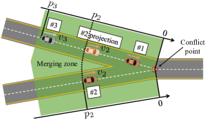
Figure 2: An example of virtual projection in the merging zone, where the CAV–$2$ is projected from the perspective of HDV–$3$.

Using the proposed prediction model, the position of each HDV in the control zone can be represented either by a cubic polynomial or by an affine function of time. The trajectory prediction is then used for estimating the HDVs’ exit times to impose the no-conflict (5) and rear-end safety constraints (6). We use $t_{k}^{\mathrm{f}}$ and ${[a_{k},b_{k},c_{k},d_{k}]}$, ${k\in\mathcal{H}(t)}$, to denote the predicted exit time and the constants parameterizing the predicted trajectory of HDV–$k$. Substituting the solution (15) into (18) (for both $p_{k}$ and $p_{j}$), the trajectory parameters of HDV–$k$ can be obtained from those of the preceding vehicle $j$ according to

$$\begin{split}a_{k}&=a_{j},\\ b_{k}&=b_{j}-3a_{j}\tau_{k},\\ c_{k}&=c_{j}+3a_{j}\tau_{k}^{2}-2b_{j}\tau_{k},\\ d_{k}&=d_{j}-a_{j}\tau_{k}^{3}+b_{j}\tau_{k}^{2}-c_{j}\tau_{k}-w\tau_{k},\end{split}$$ (19)

and $t_{k}^{\mathrm{f}}$ can be found by solving

$$a_{k}(t_{k}^{\mathrm{f}})^{3}+b_{k}(t_{k}^{\mathrm{f}})^{2}+c_{k}t_{k}^{\mathrm{f}}+d_{k}=0.$$ (20)

Then $t_{k}^{\mathrm{f}}$ and ${[a_{k},b_{k},c_{k},d_{k}]}$ can be integrated into the constraints (5) and (6) between CAV–$i$ and HDV–$k$.

III-C Safety Filter using Control Barrier Functions

Using Newell’s car-following model, we can predict the HDVs’ future trajectories and then integrate them into Problem III-A to derive the trajectory and control law for CAVs in the control zone. However, in reality, HDVs may behave differently from the predicted model. Under this discrepancy, the derived optimal control law for CAVs may not always ensure conflict-free maneuvers. To address this issue, in this subsection, we utilize control barrier functions [20] to design a safety filter that modifies the original optimal control input to a safe control action once unsafe situations are realized. Thus, conflict-free maneuvers are guaranteed for the CAVs.

To develop this safety filter, we consider a system involving a CAV–$i$ and a preceding vehicle $k$ traveling inside the control zone. Note that the preceding vehicle may be either an HDV or a CAV. Also, to ensure both rear-end safety and to avoid conflicts with vehicles on the other merging road, the preceding vehicle $j$ refers to the vehicle either physically ahead of the CAV–$i$ on the same lane, i.e., ${k=\max\,\{j\in\mathcal{S}_{i}(t_{i}^{0})\;|\;j<i\}}$, or virtually projected from the neighboring lane, i.e., ${k=\max\,\{j\in\mathcal{N}_{i}(t_{i}^{0})\;|\;j<i\}}$, whichever is the closest in front. Based on (1), the dynamics of such a system can be written as

$$\begin{split}\dot{D}_{ik}(t)&=v_{k}(t)-v_{i}(t),\\ \dot{v}_{i}(t)&=u_{i}(t),\end{split}$$ (21)

where ${D_{ik}:=p_{k}-p_{i}}$ is the distance between vehicles $i$ and $k$. By defining the state ${x:=[D_{ik}~{}v_{i}]^{\top}}$ and the input ${u:=u_{i}}$, system (21) can be rewritten into the concise form

$$\dot{x}=f(x)+g(x)u,$$ (22)

with

$$f(x)=\begin{bmatrix}v_{k}-v_{i}\\ 0\end{bmatrix},\quad g(x)=\begin{bmatrix}0\\ 1\end{bmatrix}.$$ (23)

We characterize the safety of CAV–$i$ by the forward invariance of a safe set ${\mathcal{S}\subset\mathbb{R}^{2}}$, that is, we require that ${x(0)\in\mathcal{S}\Rightarrow x(t)\in\mathcal{S}}$, $\forall t\geq 0$. We define a scalar-valued control barrier function (CBF) such that ${h(x)\geq 0}$ when ${x\in\mathcal{S}}$, that is, safety can be ensured by maintaining the positivity of the CBF. Here we define

$$\begin{split}\mathcal{S}&=\{x\in\mathbb{R}^{2}:D_{ik}\geq d_{\mathrm{sf}}+t^{\mathrm{h}}_{\mathrm{sf}}v_{i}\},\\ h(x)&=(D_{ik}-d_{\mathrm{sf}})/t^{\mathrm{h}}_{\mathrm{sf}}-v_{i},\end{split}$$ (24)

where ${d_{\mathrm{sf}}\geq 0}$ is the safe standstill distance while $t^{\mathrm{h}}_{\mathrm{sf}}$ is the safe time headway. An illustration of the safe set $\mathcal{S}$ is shown in Fig. 3 where $t^{\mathrm{h}}_{\mathrm{sf}}$ and $d_{\mathrm{sf}}$ are indicated.

It was shown in [21] that since ${\nabla h(x)g(x)<0}$ always holds, the positivity of the CBF defined in (24) can be assured if the control action satisfies

$$u\leq u_{\mathrm{s}}(x)=-\frac{\nabla h(x)f(x)+\alpha(h(x))}{\nabla h(x)g(x)},$$ (25)

with ${\alpha>0}$. Substituting (23) and (24) into (25) we obtain

$$u_{\mathrm{s}}(x)=\frac{v_{k}-v_{i}}{t^{\mathrm{h}}_{\mathrm{sf}}}+\alpha\bigg{(}\frac{D_{ik}-d_{\mathrm{sf}}}{t^{\mathrm{h}}_{\mathrm{sf}}}-v_{i}\bigg{)}.$$ (26)

Such safe control input can upper bound the CAVs’ control inputs. In particular, denoting the optimal control input derived from Problems III-A and III-A as $u_{\mathrm{o}}$, a safety filter can be synthesized as

$$u=\min\{u_{\mathrm{o}},u_{\mathrm{s}}\},$$ (27)

which modifies the original optimal control input $u_{\mathrm{o}}$ to safe input $u_{\mathrm{s}}$ in a minimally invasive fashion. This ensures CAVs’ conflict-free maneuvers under uncertain HDVs’ behaviors.

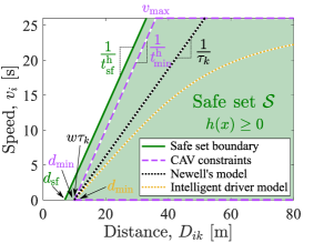
Figure 3: Safe set $\mathcal{S}$ (green region) visualized in state space for ${t^{\mathrm{h}}_{\mathrm{sf}}=1}$ $[\mathrm{s}]$ and ${d_{\mathrm{sf}}=7}$ $[\mathrm{m}]$. The range policies corresponding to the CAV constraints (3) and (6) (purple dashed), Newell’s car following model (18) (black dotted) and the intelligent driver model (28) (yellow dotted) are also indicated.

IV Simulation Results

In this section, we demonstrate the proposed framework by numerical simulations under various penetration rates of CAVs and various traffic volumes. We consider a merging scenario for a control zone of length $300\text{\,}\mathrm{m}$, and we define a merging zone of length $75\text{\,}\mathrm{m}$ upstream of the conflict point. Vehicles enter the control zone with uniformly randomized initial speeds between $22$ and $26\text{\,}\mathrm{m}\mathrm{/}\mathrm{s}$. We generate random vehicle entering time by a normal distribution where the traffic volumes determine the mean.

Given a preceding vehicle $j$ (which may be projected from the neighboring road), the following HDV–$k$’s control input is given by

$$\!u_{k}\!=a\Bigg{(}\!1-\bigg{(}\!\frac{v_{k}}{v_{\max}}\!\bigg{)}^{4}\!-\!\Bigg{(}\!\frac{d_{\min}+t^{\mathrm{h}}v_{k}-\frac{v_{k}(v_{j}-v_{k})}{2\sqrt{ab}}}{p_{j}-p_{k}}\!\Bigg{)}^{2}\Bigg{)},$$ (28)

where $v_{\max}$ and $d_{\min}$ are the same as the speed limit and the standstill distance imposed for CAVs in (3) and (6) but here these denote desired values rather than constraints. Also, $t^{\mathrm{h}}$ is the desired time headway, $a$ is the desired maximum acceleration, and $b$ is the comfortable deceleration. The parameters used in the simulations are ${u_{\mathrm{min}}=$-3\text{\,}\mathrm{m}\mathrm{/}\mathrm{s}^{2}$}$, ${u_{\mathrm{max}}=$2\text{\,}\mathrm{m}\mathrm{/}\mathrm{s}^{2}$}$, ${v_{\mathrm{max}}=$26\text{\,}\mathrm{m}\mathrm{/}\mathrm{s}$}$, ${t_{\min}=$2\text{\,}\mathrm{s}$}$, ${d_{\min}=$10\text{\,}\mathrm{m}$}$, ${t^{\mathrm{h}}_{\min}=$1\text{\,}\mathrm{s}$}$, ${d_{\mathrm{sf}}=$7\text{\,}\mathrm{m}$}$, ${t^{\mathrm{h}}_{\mathrm{sf}}=$1\text{\,}\mathrm{s}$}$, ${\alpha=$0.6\text{\,}\mathrm{1}\mathrm{/}\mathrm{s}$}$, ${t^{\mathrm{h}}=$2\text{\,}\mathrm{s}$}$, ${a=$1\text{\,}\mathrm{m}\mathrm{/}\mathrm{s}^{2}$}$, and ${b=$1.5\text{\,}\mathrm{m}\mathrm{/}\mathrm{s}^{2}$}$.

On the state space diagram in Fig. 3, we plot the range policy embedded in the IDM and compare it with Newell’s car-following model (using the most aggressive $\tau_{k}$ value obtained from simulations). Both lie inside the safe set $\mathcal{S}$. We also remark that for simplicity of the simulation, when a feasible solution of Problems III-A and III-A does not exist at the entrance of the control zone, the safe controller $u_{\mathrm{s}}$ is used for the CAV, instead of numerically solving a two-level optimization problem to derive $u_{\mathrm{o}}$.

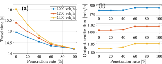
Figure 4: Average travel time (a) and output traffic flux (b) under different penetration rates of coordinated CAVs.

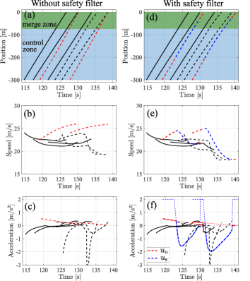
Figure 5: Simulated position, speed, and acceleration profiles for a CAV and surrounding HDVs without and with CBF-based safety filter. The trajectories of HDVs are represented by black curves. For CAV, red segments denote where optimal control input $u_{\mathrm{o}}$ is used while blue segments denote where safe input $u_{\mathrm{s}}$ is used. The actual control input used for the CAV is highlighted by the thick curve in panel (f). The vehicles moving on different roads are distinguished by solid and dashed curves. The blue and green shaded areas highlight the control and merge zones.

We conduct simulations using the proposed framework for six CAV penetration rates: 0%, 20%, 40%, 60%, 80%, 100%, and three traffic volumes: $1000$, $1200$, and $1400$ vehicles per hour. To quantify the benefits of coordinated CAVs, we use two metrics: average travel time in the control zone of the vehicles and the output traffic flux of the vehicles exiting the control zone. We conduct the simulations with 200 vehicles to compute these two metrics. In Fig. 4, we summarize the results of average travel time and output flux for different CAV penetration rates and traffic volumes. Note that by increasing the CAV penetration rate, the average travel time improves significantly. Under high traffic volume ($1400\text{\,}\mathrm{v}\mathrm{e}\mathrm{h}\mathrm{/}\mathrm{h}$), $100\%$ coordinated CAVs can improve the average travel time by $11\%$ compared to the baseline traffic with pure HDVs. Moreover, with higher CAV penetration, we also observe moderate improvements in the output traffic flux; see Fig. 4(b).

To demonstrate the CBF-based safety filter, the position, speed, and acceleration profiles of a few CAVs and HDVs are shown in Fig. 5 for traffic volume $1200\text{\,}\mathrm{v}\mathrm{e}\mathrm{h}\mathrm{/}\mathrm{h}$. The left panels reveal that without the safety filter, the optimal trajectories of the CAVs (red curves), derived at the entry of the control zone, may come very close to the trajectories of the HDVs (black curves). On the other hand, the right panels demonstrate that with the help of the safety filter, the CAVs can avoid conflicts with the HDVs. Note that in panels (d) and (e), the red segments represent where the optimal control input $u_{\mathrm{o}}$ is used for the CAV, while the blue segments represent where the safe input $u_{\mathrm{s}}$ is used. In panel (f), the control inputs $u_{\mathrm{o}}$ and $u_{\mathrm{s}}$ are plotted in red and blue, respectively, with the overall control input that the CAV used highlighted by the thicker curve.

V Concluding Remarks

In this paper, we presented a framework for coordinating CAVs in mixed traffic where they interact with HDVs. We developed an upper-level optimization problem that yields the minimum travel time of the CAVs and uses the unconstrained trajectory solution of a low-level energy-optimal control problem. We utilized Newell’s car-following model with virtual projection to predict human driving behavior and introduced a control barrier function-based safety filter to address possible unsafe situations arising from the inaccuracy of these predictions. Numerical simulations were used to demonstrate the performance and implications of the proposed framework. Future research should address the problem of merging scenarios with multiple lanes and conduct experimental validation to assess the real-time practicality of the proposed framework.

References

- [1] T. Ersal, I. Kolmanovsky, N. Masoud, N. Ozay, J. Scruggs, R. Vasudevan, and G. Orosz, “Connected and automated road vehicles: state of the art and future challenges,” Vehicle System Dynamics, vol. 58, no. 5, 2020.
- [2] A. A. Malikopoulos, L. E. Beaver, and I. V. Chremos, “Optimal time trajectory and coordination for connected and automated vehicles,” Automatica, vol. 125, no. 109469, 2021.
- [3] J. I. Ge and G. Orosz, “Optimal control of connected vehicle systems with communication delay and driver reaction time,” IEEE Transactions on Intelligent Transportation Systems, vol. 18, no. 8, pp. 2056–2070, 2017.
- [4] B. Chalaki, L. E. Beaver, and A. A. Malikopoulos, “Experimental validation of a real-time optimal controller for coordination of cavs in a multi-lane roundabout,” in IEEE Intelligent Vehicles Symposium (IV), 2020, pp. 504–509.
- [5] A. Katriniok, B. Rosarius, and P. Mähönen, “Fully distributed model predictive control of connected automated vehicles in intersections: Theory and vehicle experiments,” IEEE Transactions on Intelligent Transportation Systems, vol. 23, no. 10, pp. 18 288–18 300, 2022.
- [6] B. Chalaki and A. A. Malikopoulos, “A barrier-certified optimal coordination framework for connected and automated vehicles,” in Proceedings of the 61th IEEE Conference on Decision and Control (CDC), 2022, pp. 2264–2269.
- [7] B. Chalaki, L. E. Beaver, B. Remer, K. Jang, E. Vinitsky, A. Bayen, and A. A. Malikopoulos, “Zero-shot autonomous vehicle policy transfer: From simulation to real-world via adversarial learning,” in 16th IEEE International Conference on Control & Automation (ICCA), 2020, pp. 35–40.
- [8] B. Chalaki and A. A. Malikopoulos, “A hysteretic q-learning coordination framework for emerging mobility systems in smart cities,” in 2021 European Control Conferences (ECC), 2021, pp. 17–22.
- [9] “Social Interactions for Autonomous Driving: A Review and Perspectives,” Foundations and Trends® in Robotics, vol. 10, no. 3-4, pp. 198–376, 2022.
- [10] B. M. Albaba and Y. Yildiz, “Modeling cyber-physical human systems via an interplay between reinforcement learning and game theory,” Annual Reviews in Control, vol. 48, pp. 1–21, 2019.
- [11] M. Karimi, C. Roncoli, C. Alecsandru, and M. Papageorgiou, “Cooperative merging control via trajectory optimization in mixed vehicular traffic,” Transportation Research Part C, vol. 116, p. 102663, 2020.
- [12] A. Bajcsy, S. L. Herbert, D. Fridovich-Keil, J. F. Fisac, S. Deglurkar, A. Dragan, and C. Tomlin, “A scalable framework for real-time multi-robot, multi-human collision avoidance,” International Conference on Robotics and Automation (ICRA), pp. 936–943, 2019.
- [13] M. Koschi and M. Althoff, “Set-based prediction of traffic participants considering occlusions and traffic rules,” IEEE Transactions on Intelligent Vehicles, vol. 6, no. 2, pp. 249–265, 2021.
- [14] S. Oh, Q. Chen, H. E. Tseng, G. Pandey, and G. Orosz, “Adaptive signalized intersection control in mixed traffic environment of connected vehicles with safety guarantees,” in 26th IEEE International Conference on Intelligent Transportation Systems (ITSC), 2023.
- [15] B. Chalaki, L. E. Beaver, A. M. I. Mahbub, H. Bang, and A. A. Malikopoulos, “A research and educational robotic testbed for real-time control of emerging mobility systems: From theory to scaled experiments,” IEEE Control Systems, vol. 42, no. 6, pp. 20–34, 2022.
- [16] N. Buckman, A. Pierson, W. Schwarting, S. Karaman, and D. Rus, “Sharing is caring: Socially-compliant autonomous intersection negotiation,” in IEEE/RSJ International Conference on Intelligent Robots and Systems (IROS). IEEE, 2019, pp. 6136–6143.
- [17] H. Liu, W. Zhuang, G. Yin, Z. Li, and D. Cao, “Safety-critical and flexible cooperative on-ramp merging control of connected and automated vehicles in mixed traffic,” IEEE Transactions on Intelligent Transportation Systems, 2023.
- [18] M. Faris, P. Falcone, and J. Sjöberg, “Optimization-based coordination of mixed traffic at unsignalized intersections based on platooning strategy,” in IEEE Intelligent Vehicles Symposium (IV), 2022, pp. 977–983.
- [19] G. F. Newell, “A simplified car-following theory: a lower order model,” Transportation Research Part B, vol. 36, no. 3, pp. 195–205, 2002.
- [20] A. Alan, A. J. Taylor, C. R. He, A. D. Ames, and G. Orosz, “Control barrier functions and input-to-state safety with application to automated vehicles,” IEEE Transactions on Control Systems Technology, 2023, https://doi.org/10.1109/TCST.2023.3286090.
- [21] T. G. Molnár, G. Orosz, and A. D. Ames, “On the safety of connected cruise control: analysis and synthesis with control barrier functions,” in 62nd IEEE Conference on Decision and Control (CDC), 2023, https://arxiv.org/abs/2309.00074.
- [22] M. Shen, C. R. He, T. G. Molnar, A. H. Bell, and G. Orosz, “Energy-efficient connected cruise control with lean penetration of connected vehicles,” IEEE Transactions on Intelligent Transportation Systems, 2023, https://doi.org/10.1109/TIV.2023.3281763.
- [23] A. A. Malikopoulos, C. G. Cassandras, and Y. J. Zhang, “A decentralized energy-optimal control framework for connected automated vehicles at signal-free intersections,” Automatica, vol. 93, pp. 244–256, 2018.
- [24] T. G. Molnár, X. A. Ji, S. Oh, D. Takács, M. Hopka, D. Upadhyay, M. Van Nieuwstadt, and G. Orosz, “On-board traffic prediction for connected vehicles: implementation and experiments on highways,” in American Control Conference (ACC), 2022, pp. 1036–1041.
- [25] A. I. M. Medina, N. van de Wouw, and H. Nijmeijer, “Automation of a T-intersection using virtual platoons of cooperative autonomous vehicles,” in 18th IEEE International Conference on Intelligent Transportation Systems (ITSC), 2015, pp. 1696–1701.
- [26] Y. Guo, Q. Sun, R. Fu, and C. Wang, “Improved car-following strategy based on merging behavior prediction of adjacent vehicle from naturalistic driving data,” IEEE Access, vol. 7, pp. 44 258–44 268, 2019.