Adapting to Disruptions: Flexibility as a Pillar of Supply Chain Resilience

Abstract

Supply chain disruptions cause shortages of raw material and products. To increase resilience, i.e., the ability to cope with shocks, substituting goods in established supply chains can become an effective alternative to creating new distribution links. We demonstrate its impact on supply deficits through a detailed analysis of the US opioid distribution system. Reconstructing 40 billion empirical distribution paths, our data-driven model allows a unique inspection of policies that increase the substitution flexibility. Our approach enables policymakers to quantify the trade-off between increasing flexibility, i.e., reduced supply deficits, and increasing complexity of the supply chain, which could make it more expensive to operate.

Introduction

The complexity of supply chains—connecting manufacturers, distributors, retailers, and final buyers—has increased over the past century, raising concerns about their resilience [3]. Recent events such as the COVID-19 pandemic, the war in Ukraine, and US–China trade disputes have affected supply chains by severely disrupting the global distribution of raw materials and goods. Following the Covid-19 pandemic, the US administration declared the “Public Health Supply Chain” a top national security issue and is seeking “new approaches to build diversity and flexibility” [30]. To do so, policymakers and firms must quantify and devise policies to improve resilience, which is the ability to mitigate shortages following sudden reductions in products’ availability.

There are several ways to tackle product shortages [27, 11]. However, only two responses are immediately available: rationing and substitution. While rationing may become necessary as the shortage deepens, substitution is typically the first choice as it impacts final buyers the least. A distributor has two strategies to implement substitution: (i) establishing relations with new distributors, or (ii) leveraging existing relations to obtain a substitute good.

The first strategy requires searching for new distributors and establishing new business relations, which may be costly and time-consuming [25]. The second strategy requires relaxing product preferences by accepting substitute goods from existing upstream distributors. Inspired by the seminal works of Tang and Tomlin [24], Dolgui et al. [5], Ivanov et al. [10], we call this last strategy flexibility. We show that policies fostering flexibility can considerably alleviate shortages.

An ideal dataset to study the power of flexibility is ARCOS [22]. It lists all drug shipments from 2006 to 2014 in the US opioid distribution system that has been often affected by shortages with dramatic consequences [26, 32, 13, 29, 8]. This dataset offers an unprecedented view of distribution at a systemic scale, which is unique in supply chain research [1]. With these data, we reconstruct 40 billion distribution paths connecting manufacturers to more than a thousand distributors and 200 000 final buyers, i.e., pharmacies, hospitals, and practitioners. Based on the reconstructed paths, we develop and estimate a data-driven model to investigate (i) how supply shocks lead to shortages and (ii) how fostering flexibility mitigates them.

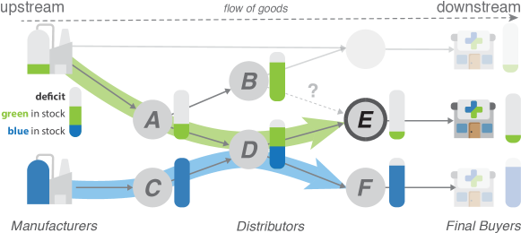
Figure 1: Schematic illustration of a distribution system of two perfectly substitutable products: blue and green. Goods flow from upstream to downstream distributors, and orders in the opposite direction. Grey arrows represent shipments of goods from one distributor to another. The two bold coloured arrows are distribution paths, i.e., sequences of distributors through which goods arrive at their destination (final buyers). In this example, there is a shortage of green, shown by the deficit of green at both distributors and final buyers, while blue is fully available. Distributor $E$ has demand for green, exceeding the stock available upstream at $D$. $D$ could satisfy the demand with blue, a substitute. This is only possible if $E$ relaxes its upstream preference for green and accepts blue instead. Alternatively, $E$ could establish a new relation with $B$ to obtain green (dashed line). Assuming that the cost of establishing a new relation is higher than substituting blue for green, $E$ should choose the latter. This work focuses on this substitution, i.e., relaxing upstream preferences.

Upstream Preferences and Flexibility

To operationalize flexibility in a distribution system, we focus on the distributor of a good rather than the good itself. To understand this change of perspective consider the example in Fig. 1. It shows a distribution system of two substitutable goods: green and blue. Distributor $E$ prefers goods coming from $A$ (green) over $C$ (blue). We formalize these upstream preferences as stochastic chains with memory [15, 2]. These correspond to the probabilities that $E$ places an order to $D$ for goods coming from $A$ or $C$. In this case, $\Pr(E\mathrel{\hbox{\rule[-0.2pt]{5.0pt}{0.4pt}}\mkern-4.0mu\hbox{\char 41\relax}}D\mathrel{\hbox{\rule[-0.2pt]{5.0pt}{0.4pt}}\mkern-4.0mu\hbox{\char 41\relax}}A)=1$ and $\Pr(E\mathrel{\hbox{\rule[-0.2pt]{5.0pt}{0.4pt}}\mkern-4.0mu\hbox{\char 41\relax}}D\mathrel{\hbox{\rule[-0.2pt]{5.0pt}{0.4pt}}\mkern-4.0mu\hbox{\char 41\relax}}C)=0$, respectively. However, if $E$ had no specific preferences regarding $A$ (green) or $C$ (blue), it would instead receive goods solely based on their availability in $D$. This implies that $E$ would adapt to the preferences of its upstream distributor $D$. Thus, $\Pr(E\mathrel{\hbox{\rule[-0.2pt]{5.0pt}{0.4pt}}\mkern-4.0mu\hbox{\char 41\relax}}D\mathrel{\hbox{\rule[-0.2pt]{5.0pt}{0.4pt}}\mkern-4.0mu\hbox{\char 41\relax}}A)=\Pr(D\mathrel{\hbox{\rule[-0.2pt]{5.0pt}{0.4pt}}\mkern-4.0mu\hbox{\char 41\relax}}A)=0.5$ and $\Pr(E\mathrel{\hbox{\rule[-0.2pt]{5.0pt}{0.4pt}}\mkern-4.0mu\hbox{\char 41\relax}}D\mathrel{\hbox{\rule[-0.2pt]{5.0pt}{0.4pt}}\mkern-4.0mu\hbox{\char 41\relax}}C)=\Pr(D\mathrel{\hbox{\rule[-0.2pt]{5.0pt}{0.4pt}}\mkern-4.0mu\hbox{\char 41\relax}}C)=0.5$. Flexibility $\phi_{E}$ is the propensity of distributor $E$ to relax its preferences in favour to those upstream. Formally,

$$\Pr(E\mathrel{\hbox{\rule[-0.2pt]{5.0pt}{0.4pt}}\mkern-4.0mu\hbox{\char 41\relax}}D\mathrel{\hbox{\rule[-0.2pt]{5.0pt}{0.4pt}}\mkern-4.0mu\hbox{\char 41\relax}}A|\phi_{E}) :=\phi_{E}\Pr(E\mathrel{\hbox{\rule[-0.2pt]{5.0pt}{0.4pt}}\mkern-4.0mu\hbox{\char 41\relax}}D\mathrel{\hbox{\rule[-0.2pt]{5.0pt}{0.4pt}}\mkern-4.0mu\hbox{\char 41\relax}}A)+(1-\phi_{E})\Pr(D\mathrel{\hbox{\rule[-0.2pt]{5.0pt}{0.4pt}}\mkern-4.0mu\hbox{\char 41\relax}}A)$$ (1)

$$\Pr(E\mathrel{\hbox{\rule[-0.2pt]{5.0pt}{0.4pt}}\mkern-4.0mu\hbox{\char 41\relax}}D\mathrel{\hbox{\rule[-0.2pt]{5.0pt}{0.4pt}}\mkern-4.0mu\hbox{\char 41\relax}}C|\phi_{E}) :=\phi_{E}\Pr(E\mathrel{\hbox{\rule[-0.2pt]{5.0pt}{0.4pt}}\mkern-4.0mu\hbox{\char 41\relax}}D\mathrel{\hbox{\rule[-0.2pt]{5.0pt}{0.4pt}}\mkern-4.0mu\hbox{\char 41\relax}}C)+(1-\phi_{E})\Pr(D\mathrel{\hbox{\rule[-0.2pt]{5.0pt}{0.4pt}}\mkern-4.0mu\hbox{\char 41\relax}}C)\;.$$

When $\phi_{E}>0$, distributor $E$ becomes more flexible in its preferences and starts sourcing goods from $C$, thus opening up an alternative distribution path: $C\mathrel{\hbox{\rule[-0.2pt]{5.0pt}{0.4pt}}\mkern-4.0mu\hbox{\char 41\relax}}D\mathrel{\hbox{\rule[-0.2pt]{5.0pt}{0.4pt}}\mkern-4.0mu\hbox{\char 41\relax}}E$. Through this new path, $E$ can fulfill its demand by substituting the good (green) it needs with the substitute (blue) coming from $C$. For instance, suppose E has a deficit of 4 green units, and D has a total stock of 4 units (2 green and 2 blue). If $\phi_{E}=0$, E would only be able to fulfill 2 units of its demand by receiving 2 green units. Instead, if $E$ partially relaxes its upstream preferences ($\phi_{E}=0.5$), $E$ could further reduce its deficit by an additional unit.

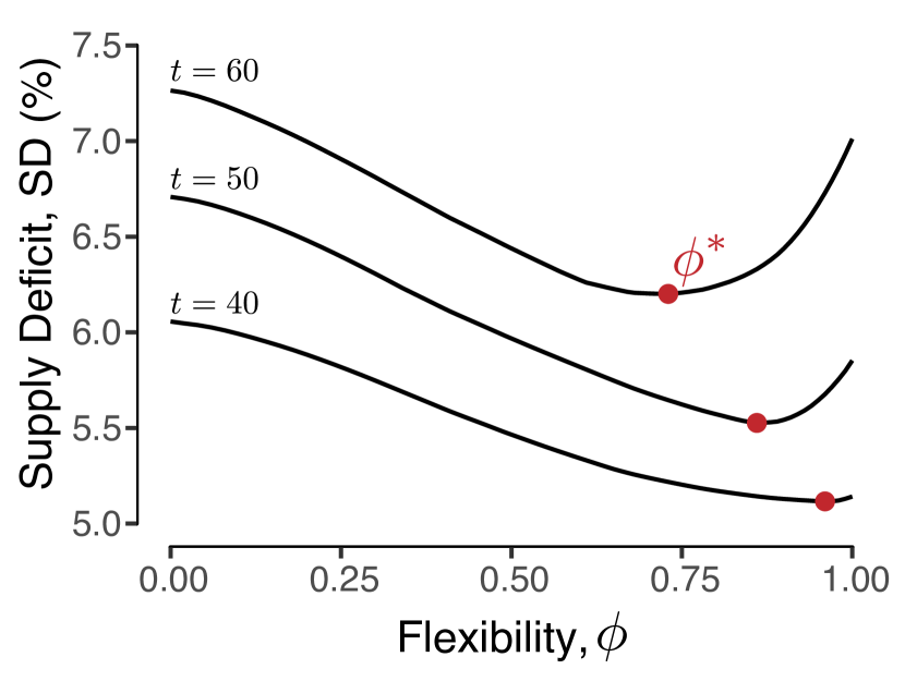
(a)

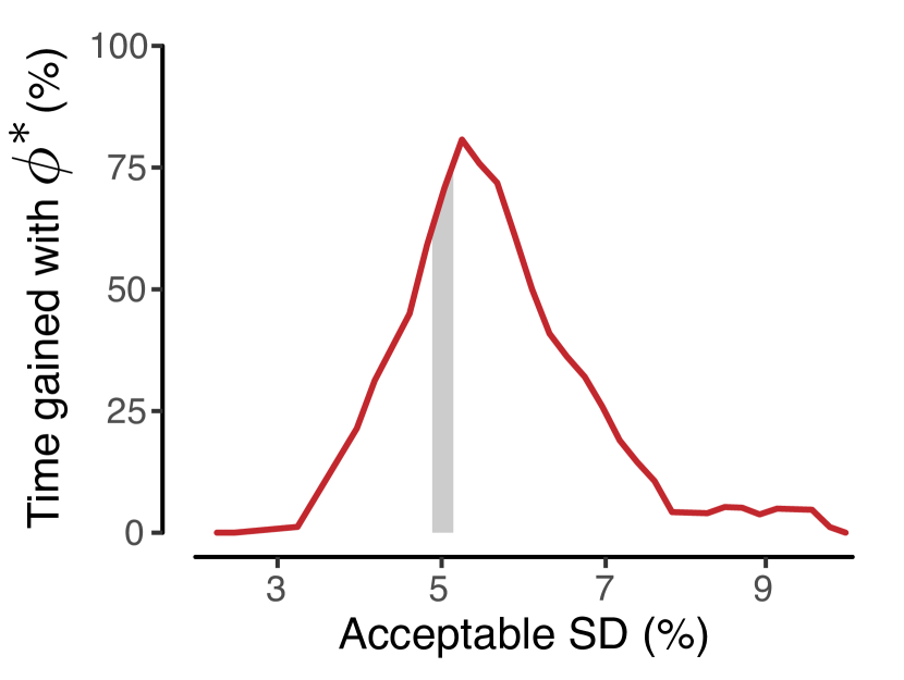
(c)

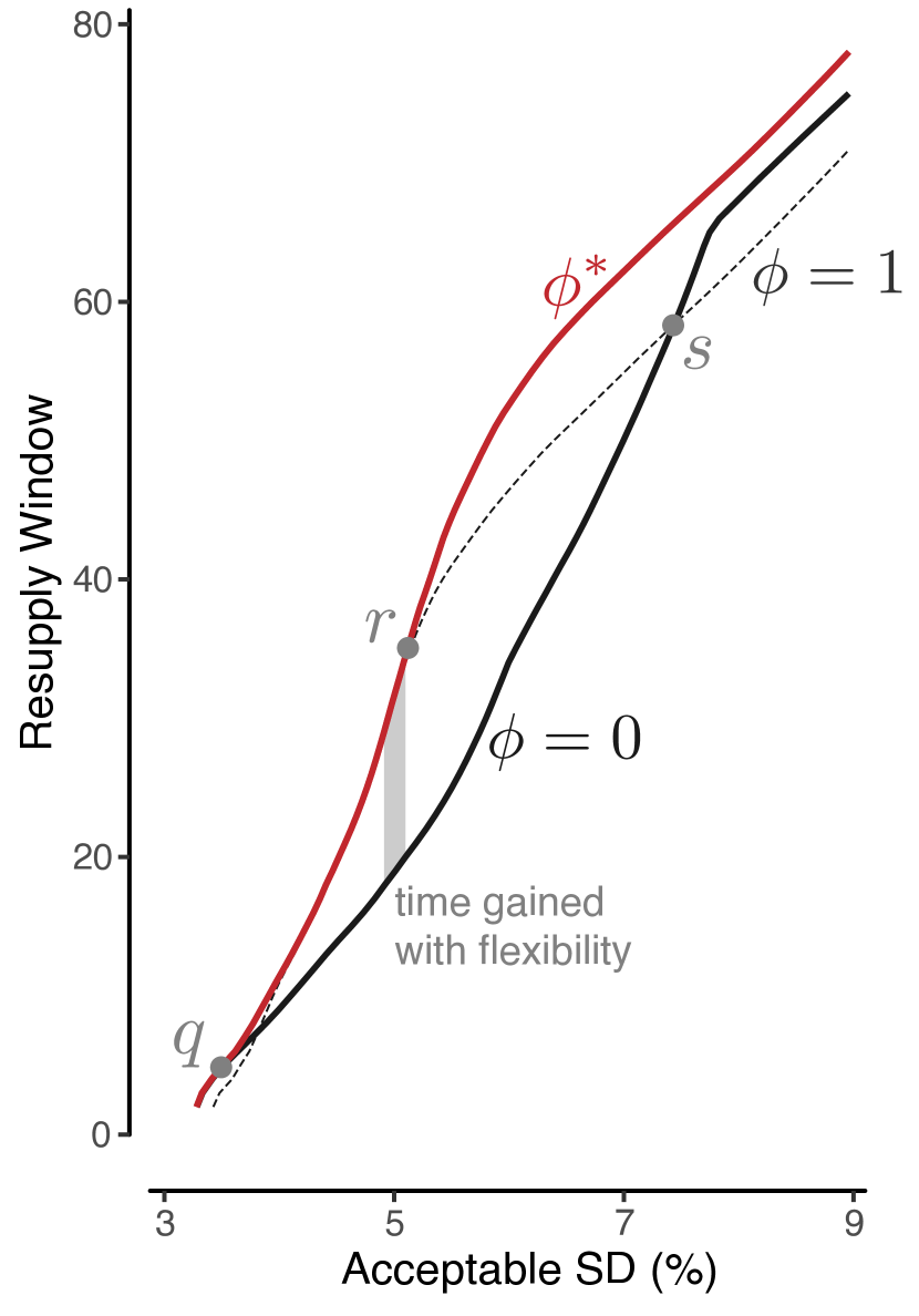
(b)

Figure 3: Stress-test simulation results for the Oxycodone distribution system in 2012. (a) Percentage of final buyers’ total demand that was not met, shown as the deficit, for flexibility values $\phi\in[0,1]$. The results are plotted at 40, 50, and 60 days after production stopped. The flexibility value $\phi^{*}$ yielding the maximum deficit reduction is shown in red. (b) Available resupply window shown as the time available to resupply before breaching an acceptable supply deficit (ASD), black line. The extended resupply window obtained with $\phi=\phi^{*}$ shown in red, is always above the black line. The resupply window obtained with full flexibility ($\phi=1$) is shown as the dashed line. Up to point $q$, the resupply window is the same for $\phi=0$ and $\phi^{*}$. Beyond point $r$, the largest resupply window is obtained for $\phi^{*}<1$. Beyond point $s$, full flexibility ($\phi=1$) is worse than no flexibility ($\phi=0$). (c) Time gained with flexibility, showing the increase in the time available for resupply for a given ASD.

Flexibility alleviates shortages

Stress test of distribution systems

We use stress test simulations to explore how the empirical distribution system may respond to supply shocks. Using a data-driven agent-based model, we simulate distributors placing orders based on demand and distributing goods based on orders. To simulate a sudden stop in production at $t=0$, we set upstream distributor stocks to only 70% of their maximal capacity inferred from data. We then analyze how this upstream deficit affects the final-buyers supply deficit and how the latter grows over time while production is halted. See Section 1.5 for a detailed explanation of the simulations.

In Fig. 3, we plot the outcome of the simulations for the Oxycodone distribution system. Figure 3(a) shows final-buyers supply deficit at different times. After 40 days, without flexibility, final buyers suffer a deficit of 6%. While this number might seem small, it corresponds to over $3$M missing Oxycodone doses. This deficit continues to increase with time as the shortage remains unresolved and stocks are depleted.

Mitigating supply deficit

We consider how different levels of flexibility affect the final-buyer supply deficit varying $\phi$ between 0 and 1. We assign the same flexibility $\phi$ to all distributors. In Fig. 3(a), we show that flexibility considerably reduces the deficit of final buyers. At $t$=40, the deficit decreases from about 6% to 5% as $\phi$ increases from 0 to 1. This reduction means that about $500$k more Oxycodone doses are now reaching final buyers thanks to flexibility. The largest reduction happens for some value $\phi^{*}$, corresponding to the $\phi$ value yielding the lowest supply deficit. Importantly, we find that $\phi^{*}$ may be smaller than 1.

Acceptable Supply Deficit

For essential goods, such as pharmaceuticals, a minimal supply level must be guaranteed. We use the term acceptable supply deficit (ASD) to refer to the maximum amount of goods that can be missing while still maintaining established standards. In the case of Oxycodone, an acceptable supply deficit (ASD) would be the maximum deficit that does not compromise patient safety. The concept of ASD is similar to that of service level agreements (SLAs), which set performance guarantees at the company level. However, ASD differs from SLAs in that it is a systemic measure considering all final buyers.

Given an ASD, we define the resupply window as the latest possible time $t$ at which resupply must happen before the deficit exceeds the ASD. We find that the resupply window can be considerably extended thanks to flexibility. In Fig. 3(b), we show the maximum extension of the resupply window with flexibility for a given ASD. For small ASDs, the gain from flexibility is minimal. However, for larger values, the resupply window can be substantially extended. For example, if a supply deficit of 5% is acceptable, the resupply must happen within 20 days without flexibility. With enough flexibility, the resupply window can be extended by up to 38 days.

In Fig. 3(c), we show the percentage gain that can be obtained for different levels of ASD. We find that the resupply window can be extended by up to 80%. However, if the ASD is very low, e.g., 2%, then this ASD will be breached quickly. Thus, flexibility has no time to alleviate shortages. If the ASD is very high, e.g., 10%, when that supply deficit is reached, stocks will be depleted by regular demand. Hence, we identify a range of ASD where flexibility is particularly effective.

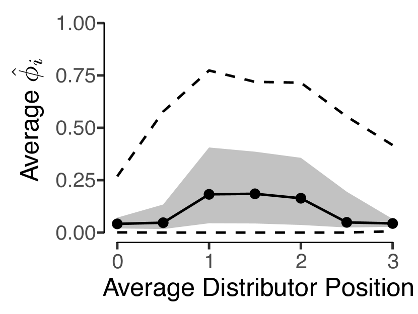
(a)

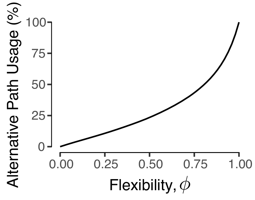
(b)

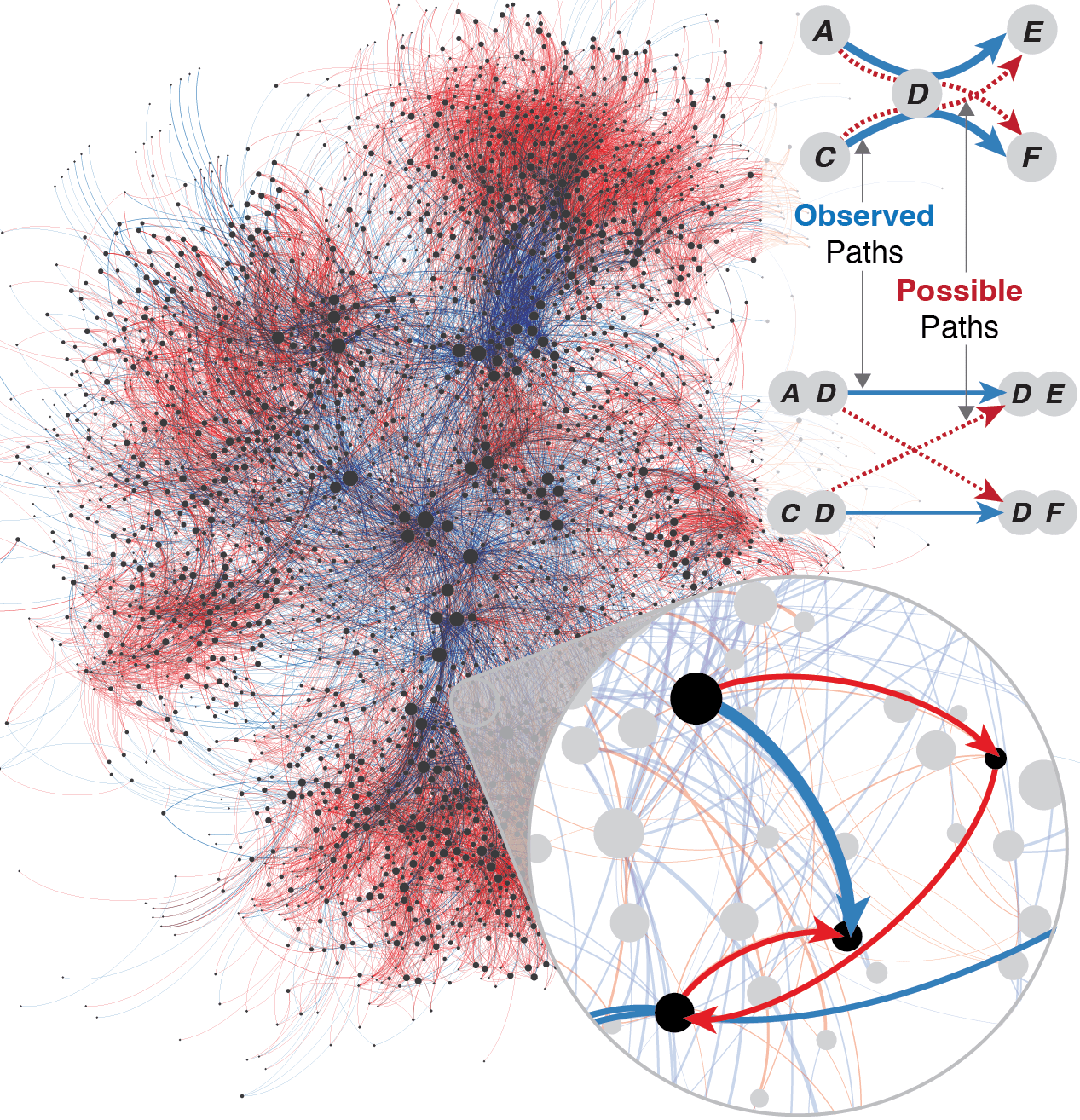
(c)

Figure 5: (a) Year-to-year flexibility $\hat{\phi}_{i}$ of distributor $i$ in the Oxycodone distribution system from 2006 to 2014, shown as a function of the distributor’s position on the distribution paths. The black lines represent the average flexibility, the shaded area shows the middle 50% of the data, and the dashed line shows 95%. (b) Proportion of goods shipped via alternative distribution paths 180 days after the stop in production, for different levels of flexibility $\phi$, (c) The distribution system for Oxycodone in 2012 represented as a second-order network. In this representation, a path of length two, such as $A\mathrel{\hbox{\rule[-0.2pt]{5.0pt}{0.4pt}}\mkern-4.0mu\hbox{\char 41\relax}}D\mathrel{\hbox{\rule[-0.2pt]{5.0pt}{0.4pt}}\mkern-4.0mu\hbox{\char 41\relax}}E$, is depicted by an edge between the two “meta-nodes” $(A,D)\mathrel{\hbox{\rule[-0.2pt]{5.0pt}{0.4pt}}\mkern-4.0mu\hbox{\char 41\relax}}(D,E)$ (as shown in the inset on the left). Blue edges indicate distribution paths that were observed, while the red edges represent alternative distribution paths that could exist. Increasing the parameter $\phi$ in this representation increases the probability that these red alternative paths become available for the distribution, in addition to the observed blue distribution paths. The zoom-in feature highlights that creating alternative distribution paths (red) allows previously disconnected nodes to connect. However, it is important to note that these alternative paths can be less direct than the observed blue paths, requiring products to follow longer routes.

Empirical Evidence for Flexibility

Flexibility can mitigate supply deficits. Now, we provide evidence that distributors can indeed adapt their upstream preferences and thus increase their flexibility. We look at how empirical distribution systems evolve over time and assess the year-to-year flexibility $\widehat{\phi}_{i}(y)$ of each distributor. $\widehat{\phi}_{i}(y)$ captures how much distributor $i$ relaxes its upstream preferences from year $y-1$ to year $y$. Precisely, we take a maximum likelihood approach (MLE) to infer $\widehat{\phi}_{i}(y)$ given the upstream preference in year $y-1$ and the observed distribution paths in year $y$. See Section 1.3 for details.

We find that, in every year, some degree of flexibility is present. While on average distributors’ flexibility is low, large flexibility values are sporadically observed. To understand which distributors are more flexible, we compute the average position a distributor has on their distribution paths. For example, distributor $D$ in Fig. 1 has position 2 in both the green and blue distribution path. In Fig. 5(a), we see how the average $\widehat{\phi}_{i}$ changes with positions. Distributors appearing at the beginning of paths have low flexibility, as do distributors at the end of paths, i.e., close to final buyers. Instead, distributors occupying middle positions are more flexible, with an average $\widehat{\phi}_{i}(t)$ as high as 0.25. In fact, 95% of distributors occupying intermediate positions within the distribution system have a flexibility as high as 0.75. This suggests that (i) distributors are able to adapt their preferences and (ii) maximum flexibility depends on their position.

Balancing deficit reduction and the cost of flexibility

Flexibility introduces alternative distribution paths

We compute the proportion of goods distributed through alternative paths as flexibility increases. In Fig. 5(b), we see that the usage of alternative paths grows monotonously with $\phi$. In other words, the more flexible, the more likely are distributors to use alternative distribution paths. This allows final buyers to receive goods from multiple sources.

To understand where these alternative distribution paths are introduced, we visualise the distribution system in Fig. 5(c). Blue edges show empirical distribution paths, while red edges represent the alternative paths available with full flexibility, i.e., $\phi=1$. The zoom-in feature in Fig. 5(c) shows that adding alternative paths (red) allows distribution between previously disconnected distributors. Importantly, from Fig. 5(c) we learn that the bulk of alternative distribution paths made available with flexibility is located towards the periphery of the distribution system.

The price of flexibility

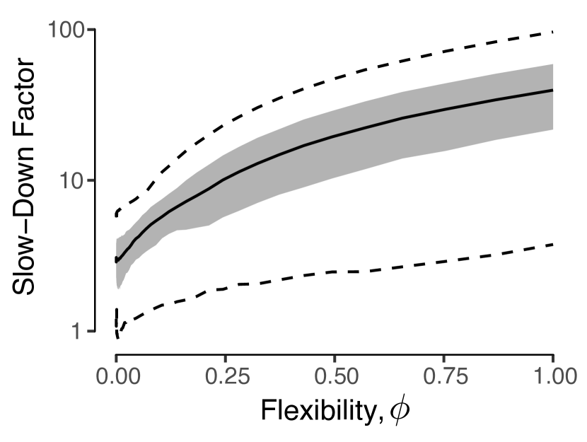
(a)

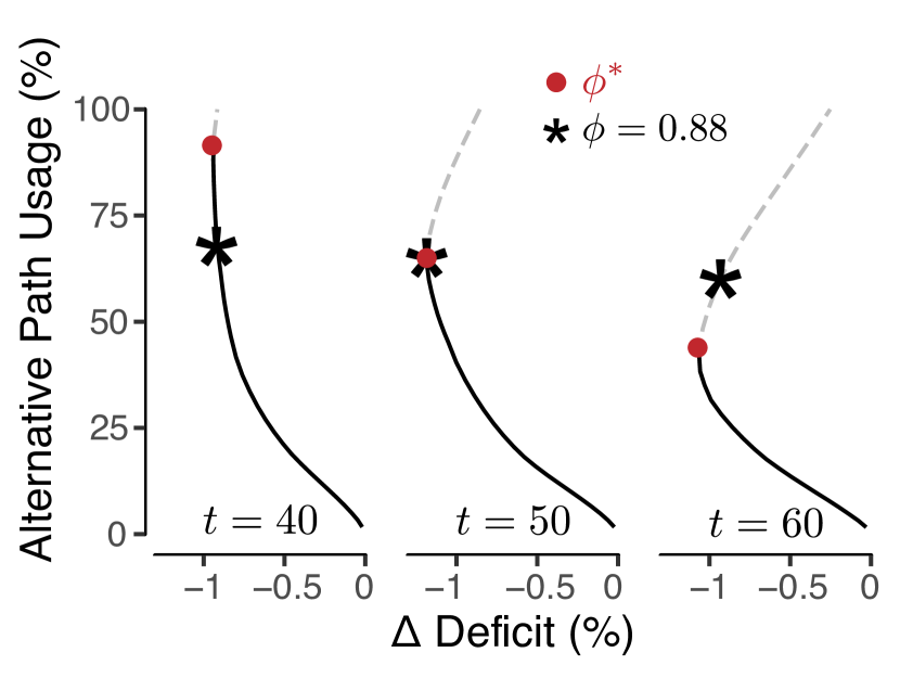
(b)

Figure 6: (a) Slow-down factor for the Oxycodone distribution system, averaged from 2007 to 2014, as a function of $\phi$. The solid line indicates the average; the dashed lines show bootstrapped 95% CI, and the shaded area indicates the 50% CI. All bootstrapped statistics are estimated over 10 000 samples. (b) Deficit Reduction ($\Delta$) versus alternative path usage, plotted at 40, 50, and 60 days after production stop. $\phi$ increases from bottom to top along the curves. Solid lines show efficient values of $\phi$, while dashed lines show inefficient ones separated at $\phi^{*}(t)$. The point corresponding to $\phi^{*}(50)$ is shown in red, which is efficient at $t=40$, has the highest deficit reduction at $t=50$, and becomes inefficient at $t=60$.

The increase in path usage may be costly. Costs may rise, for example, because of handling, labour, and increased complexity. Using alternative paths may also slow down distribution because they can be less direct, as shown in the zoom-in feature in Fig. 5(c). Therefore, alternative distribution paths may delay distribution to final buyers.

To proxy such a distribution delay, we compute the slowdown factor introduced by Scholtes et al. [17]. This factor indicates the proportion of additional distribution steps required for to reach final buyers. By modeling the distribution of goods as a diffusion process, we are able to estimate how the average distribution time scales with flexibility. Details are provided in Section 1.4.

In Fig. 6(a), we observe that increasing $\phi$ slows down the distribution system monotonously. Thus, as flexibility increases, goods pass through more distributors, potentially raising handling costs. This suggests the presence of a tradeoff between flexibility and the usage of alternative paths.

Decreasing returns to flexibility

In Fig. 6(b), we see the tradeoff between deficit reduction and alternative path usage. The plot highlights the existence of an inefficient set located on the upper side of the curves (dashed line). For points in this set, a given deficit reduction is achievable at lower flexibility as well. In other words, the same deficit is attainable using fewer distribution paths, and thus with lower costs. The set of points where this happens is the efficient set. Moreover, in Fig. 6(b) we show that an efficient point at $t=40$ becomes inefficient at $t=60$. This occurs because the value of $\phi^{*}(t)$, separating the efficient from the inefficient set, decreases with time, which is also visible in Fig. 3.

Discussion

Natural disasters, geopolitical tensions, and public health crises can severely disrupt supply chains, leading to shortages. Our work demonstrates that flexibility, i.e., the ability to substitute goods through existing distribution paths, mitigates shortages and, crucially, extends the time before a critical deficit is reached. Specifically, to quantify the distribution system’s ability to mitigate supply deficits we developed a new analysis tool for distribution systems using stochastic chains with memory [15, 2].

Strengthening supply chain resilience, i.e. the ability to withstand and recover from shocks [9, 23], was declared a top national security by US President Obama in 2012 [14]. To reconstitute the flow of commerce after disruption requires proactive and reactive measures. Proactive measures strengthen the supply chain’s ability to withstand shocks by taking preventive action before disruptions occur [4, 21], aiming to avert shortages altogether. Examples of proactive measures include mandating higher safety stocks, investing in just-in-case capacity, and pursuing diversification [26]. In contrast, reactive measures prioritize swift responses after a shortage emerges, allowing the system to adapt and mitigate the effects of the disruption [20, 18, 19]. While proactive measures may require significant upfront investments and, crucially, time, reactive measures are immediately available.

Flexibility, a reactive measure, leverages existing resources such as infrastructure, business relations, and goods, making them immediately available without creating new connections. However, flexibility is costly due to increased handling time and distribution complexity. Consequently, there is a tradeoff between its benefits and costs. To manage this tradeoff and foster flexibility, regulators and policymakers must continuously monitor distribution paths, to gain insights into how flexibility can extend the time until a critical deficit is reached.

Our work provides the necessary tools to evaluate flexibility and stress-test the system continuously. Our analysis has highlighted that the most effective flexibility level changes with time and the impact of flexibility is highest during the initial phase of a shortage. This becomes important when devising policies to foster flexibility. Our approach is applicable to a broad range of products, not just pharmaceuticals, and is well-suited for substitutable products with partially overlapping distribution systems, e.g., grain, gas and oil. By carefully balancing policies that foster flexibility and costs, supply chains can become more resilient, enabling them to adapt to disruptions.

1 Material and Methods

1.1 The ARCOS dataset

We study the opioid shipments dataset ARCOS [22], which serves as our model distribution system. The US Drug Enforcement Agency (DEA) maintains this dataset and tracks the chain of custody of every shipment of a controlled substance from manufacturing to the dispenser. ARCOS, which stands for Automated Reports and Consolidated Ordering System, is a data collection system where manufacturers and distributors report controlled substance transactions to the DEA. Transactions recorded in ARCOS include information such as the sending and receiving entities, the quantity and good shipped, and the date. Drugs are identified by their national drug code, which allows us to distinguish the labeller, good, and packaging forms, such as 12ml vials or 120 pill boxes. It is worth noting that the last entities to be tracked by ARCOS are pharmacies, hospitals, and practitioners, not the patients, and they will be referred to as “final buyers” hereafter.

Substitutability and price elasticity

The extent to which substitution alleviates shortages depends on the substitutability of the products. The FDA defines drugs to be “pharmacologically equivalent” if they contain (1) the same active ingredient, (2) have the same dosage form, and (3) are identical in strength and concentration. In this work, we follow this definition but relax the “identical in strength” and “dosage form” requirements.

Although price differences can affect product substitutability, we have chosen not to model them in this study. This decision is based on research by Yeung et al. [33], which found that medically necessary drugs, such as painkillers, are not significantly affected by short-term price increases. Furthermore, price increases do not stimulate supply, as noted by the US Food and Drug Administration in their report on drug shortages [28]. This is primarily due to the low price elasticity of prescription drugs, which is caused by how necessary pharmaceuticals are reimbursed. Insurers and federal programs, rather than patients, are usually responsible for paying for these drugs.

From shipping transactions to distribution paths

In this study, we reconstruct the distribution paths of opioid drugs by tracking all ARCOS transactions in the order they were recorded while monitoring distributor stock levels. Specifically, we trace individual packages as they leave the manufacturing facility, pass through distributors, and arrive at final buyers, e.g., hospitals, pharmacies, or practitioners.

To do so, we assume that distribution systems follow a first-in-first-out (FIFO) stock management policy, where the first packages arriving are also the first ones to leave. This policy minimizes the impact on the product’s shelf-life, which is crucial for perishable products such as medicine. In fact, the World Health Organization recommends in their "Good Distribution Practices" [31] that distributors follow a "first expiry/first-out" stock management policy.

Using the 500 million transactions in ARCOS for 2006-2014, we reconstruct 40 billion distribution paths of individual drug packages. The set of reconstructed paths is denoted as $P:=\{p_{1},p_{2},\dotsc,p_{S}\}$, where each element in the set is a single path of a single drug package. Each path is represented as a tuple $p_{s}=(M\mathrel{\hbox{\rule[-0.2pt]{5.0pt}{0.4pt}}\mkern-4.0mu\hbox{\char 41\relax}}k\mathrel{\hbox{\rule[-0.2pt]{5.0pt}{0.4pt}}\mkern-4.0mu\hbox{\char 41\relax}}j\cdots\mathrel{\hbox{\rule[-0.2pt]{5.0pt}{0.4pt}}\mkern-4.0mu\hbox{\char 41\relax}}i)$. Here, $M$ denotes a manufacturer and $k,j,i$ denotes distributors. The path ends with the last distributor that ships to the final buyers. In other words, $p_{s}$ denotes the sequence of distributors traversed by a given package on its journey from manufacturer to final buyer.

1.2 Higher-order Markov chains model for distribution systems

From distribution paths to upstream preferences

The length of reconstructed paths varies between 1 and 4. The majority of these paths, though, has a length of 2. This means that, in most cases, the distribution process involves only one manufacturer and two subsequent distributors. Given this observation, we choose to model upstream preferences up to 2 steps upstream. Supporting this assumption, LaRock et al. [12] have shown that this approach is particularly suitable to capture important paths within a system. Further, we validate this modelling choice performing the model selection tests proposed by [16, 6]. The tests show that modelling the distribution system accounting for 2 steps upstream is statistically optimal, given the available data.

Let’s consider the length-2 distribution path $p_{s}=(k\mathrel{\hbox{\rule[-0.2pt]{5.0pt}{0.4pt}}\mkern-4.0mu\hbox{\char 41\relax}}j\mathrel{\hbox{\rule[-0.2pt]{5.0pt}{0.4pt}}\mkern-4.0mu\hbox{\char 41\relax}}i)$, where $k$ is a manufacturer, and $j$ and $i$ two distributors. In our data, each length-2 path may appear as a full observation or as a subpath of a longer distribution path, i.e., $(\cdots\mathrel{\hbox{\rule[-0.2pt]{5.0pt}{0.4pt}}\mkern-4.0mu\hbox{\char 41\relax}}k\mathrel{\hbox{\rule[-0.2pt]{5.0pt}{0.4pt}}\mkern-4.0mu\hbox{\char 41\relax}}j\mathrel{\hbox{\rule[-0.2pt]{5.0pt}{0.4pt}}\mkern-4.0mu\hbox{\char 41\relax}}i\mathrel{\hbox{\rule[-0.2pt]{5.0pt}{0.4pt}}\mkern-4.0mu\hbox{\char 41\relax}}\cdots)$. We denote with $\tilde{A}_{kji}$ the total number of occurrences of $p_{s}$ in the data, summing all its occurrences as standalone path with those as subpath of longer distribution paths.

To proceed further, we assume perfect market clearing within the system. Under this assumption, supply equals demand. This implies that the amount of shipments corresponds to the orders placed. This means that $\tilde{A}_{kji}=A_{ijk}$, where $A_{ijk}$ indicates the amount of orders placed by $i$ to $k$, via the intermediary $j$. To model the distribution system, we leverage higher-order Markov chains and construct the 2-step tensor, $T^{\text{2-step}}$. Each entry of $T^{\text{2-step}}_{ijk}$ contains the probability that $i$ submits an order to $k$ via the intermediary $j$:

$$T^{\text{2-step}}_{ijk}=\frac{A_{ijk}}{\sum\limits_{j^{\prime}k^{\prime}}A_{ij^{\prime}k^{\prime}}}$$ (2)

where the sum runs over all sub-paths $(j^{\prime}\mathrel{\hbox{\rule[-0.2pt]{5.0pt}{0.4pt}}\mkern-4.0mu\hbox{\char 41\relax}}k^{\prime})$. Formally, each element of $T^{\text{2-step}}$ represents the transition probability of an order moving along a path $(i\mathrel{\hbox{\rule[-0.2pt]{5.0pt}{0.4pt}}\mkern-4.0mu\hbox{\char 41\relax}}j\mathrel{\hbox{\rule[-0.2pt]{5.0pt}{0.4pt}}\mkern-4.0mu\hbox{\char 41\relax}}k)$. $T^{\text{2-step}}$, thus, captures all upstream preferences up to 2 steps upstream. Note that Eq. 2 ensures the dependency between the (probability of) orders placed by $i$ towards $j$ and the (probability of) orders placed by $j$ towards $k$, namely $P(i\mathrel{\hbox{\rule[-0.2pt]{5.0pt}{0.4pt}}\mkern-4.0mu\hbox{\char 41\relax}}j\mathrel{\hbox{\rule[-0.2pt]{5.0pt}{0.4pt}}\mkern-4.0mu\hbox{\char 41\relax}}k)$.

Relaxing upstream preferences

Distributors may relax their upstream preferences and, in the most extreme case, accept goods independently of their origin. To capture this tendency, we introduce a 1-step transition matrix, $S$. A given element $S_{ij}$ captures the probability that $i$ places an order to $j$. Formally, we write $S_{ij}=\sum_{k}T^{\text{2-step}}_{ijk}$ where the sum runs over all distributors $k$. Using this 1-step transition matrix, we construct a new tensor, $T^{\text{1-step}}$, that captures preferences up to 1 step upstream while modelling paths of length 2:

$$T^{\text{1-step}}_{ijk}=\frac{S_{jk}}{\sum\limits_{k^{\prime}}S_{jk^{\prime}}}\cdot\Theta\left(\sum\limits_{k^{\prime}}A_{ijk^{\prime}}\right)$$ (3)

where $\Theta(x)$ equals 0 for $x\leq 0$ and equals 1 otherwise. It ensures that we only considers a distributor $j$ if there is at least one order placed by $i$ towards $j$. Note that, except for the $\Theta$, the right-hand side has only two $(jk)$ while the left-hand side of Eq. 3 has three indices $(ijk)$. This is not a mistake. We are assuming that $i$ has fully relaxed its upstream preferences, aligning them to the intermediary $j$. As a consequence, the proportion of orders that $i$ places toward $k$ does not depend on $i$ anymore, but it only depends on the proportion of orders that $j$ places toward $k$.

Flexibility

Upstream preferences are relaxed according to various level of the distributors’ flexibility. To model different levels of flexibility, we combine the $T^{\text{1-step}}_{ijk}$ and the $T^{\text{2-step}}_{ijk}$ as:

$$T(\phi_{i})_{ijk}=(1-\phi_{i})T^{\text{2-step}}_{ijk}+\phi_{i}T^{\text{1-step}}_{ijk}$$ (4)

where $\phi_{i}$ is a parameter used to interpolate between the two limit cases: (i) a fully flexible case captured by $T^{\text{1-step}}$, (ii) and a zero flexible system captured by $T^{\text{2-step}}$. Its value ranges from zero to one and indicates the percentage of goods received by distributors independently of their upstream preferences. When flexibility equals zero, $T(\phi_{i}=0)$ reduces to the 2-step tensor, i..e, $T^{\text{2-step}}$. When flexibility equals one, $T(\phi_{i}=0)$ reduces to the 1-step tensor, i.e., $T^{\text{1-step}}$.

We can visualize both $T^{\text{1-step}}$ and $T^{\text{2-step}}$ using a second order graphical representation (Fig. 5(c)). In this representation, paths of length 2 $i\mathrel{\hbox{\rule[-0.2pt]{5.0pt}{0.4pt}}\mkern-4.0mu\hbox{\char 41\relax}}j\mathrel{\hbox{\rule[-0.2pt]{5.0pt}{0.4pt}}\mkern-4.0mu\hbox{\char 41\relax}}k$ are represented by an edge between the two “meta-nodes” $(i,j)\mathrel{\hbox{\rule[-0.2pt]{5.0pt}{0.4pt}}\mkern-4.0mu\hbox{\char 41\relax}}(j,k)$ (see inset on the bottom-right of the figure). This figure shows observed paths of length two in blue, i.e., the positive entries in $T^{\text{2-step}}$. Paths, red, are possible but have not been observed and correspond to the positive entries in $T^{\text{1-step}}$. Increasing $\phi$ in this representation corresponds to adding red edges (possible paths) to the observed paths (blue edges).

1.3 Estimating the empirical flexibility

We use a maximum likelihood approach to estimate the system’s empirical flexibility at a given time horizon $h$. Specifically, we estimate the upstream preferences for each distributor by computing the shipment transition tensor $B(b,\boldsymbol{\phi})$ over a period $[t-b,t]$, where $b$ is the period over which the preferences are estimated and $\boldsymbol{\phi}$ is an n-dimensional vector whose entries $\phi_{i}$ correspond the flexibility of distributor $i$.

Specifically, we obtain $B(b,\boldsymbol{\phi})$ as the row normalized transpose of the order transition tensor $T(\boldsymbol{\phi},b)$ defined in (4). The rationale behind this is that we define expected shipments to be equal to expected orders assuming each distributor has placed orders for the observed volume. Formally,

$$B_{ijk}(b,\phi_{k}):=\frac{T_{kji}(b,\phi_{k})\cdot v_{k}}{\sum\limits_{k^{\prime}j^{\prime}}T_{k^{\prime}j^{\prime}i}(b,\phi_{k^{\prime}})\cdot v_{k^{\prime}}}$$ (5)

where $T_{ijk}(b,\phi_{k})$ is defined in (4) over the period $[t-b,t]$ and $v_{k}=\sum_{lm}A_{klm}$ is the total volume ordered by $k$.

We then construct from the shipments observed in the period $[t,t+h]$ the shipment tensor $\tilde{A}(h)$. The entry $\tilde{A}_{ijk}(h)$ captures the number of shipments from $i$ to $k$ via $j$ in the period $[t,t+h]$. Finally, we compute the likelihood of the observed shipments given the estimated transition tensor $B(b,\boldsymbol{\phi})$ parametrized by $\boldsymbol{\phi}$ as:

$$\mathcal{L}(\phi)=\prod\limits_{i,j,k}B_{ijk}(b,\phi_{k})^{\tilde{A}_{ijk}(h)}\propto\log\mathcal{L}(\phi)=\sum\limits_{i,j,k}\tilde{A}_{ijk}(h)\log B_{ijk}(b,\phi_{k})$$ (6)

The most likely parameter to have generated the observed shipments corresponds to the flexibility vector $\boldsymbol{\hat{\phi}}$ for which the likelihood is maximal.

$$\boldsymbol{\hat{\phi}}=\arg\max\limits_{\boldsymbol{\phi}}\log\mathcal{L}(\boldsymbol{\phi})$$ (7)

In Fig. 5(a), we estimate upstream preferences over a year ($b=$ 1 year) and then use the estimated transition matrix to predict the shipments over the next year ($h=$ 1 year).

1.4 Slow-down factor

To compare the distribution speed between flexible and strict upstream preferences, we employ the slow-down factor introduced by Scholtes et al. [17]. Let $M$ denote a row-stochastic transition matrix describing a random walk on a network. It has been shown that the time $t$ needed for the node visitation probability to converge to the stationary distribution starting from any initial condition scales with

$$t\approx\frac{1}{\log{\abs{\lambda_{2}\left[M\right]}}}\,,$$ (8)

where $\lambda_{2}\left[M\right]$ is the second leading eigenvalue of $M$.

Consider now the $B(b,\boldsymbol{\phi})$ tensor defined in Eq. 5 and by setting the vector $v=\mathbb{1}$. Its elements $B_{ijk}(b,\boldsymbol{\phi})$ are the probabilities of a shipment from $i$ to $k$ via $j$ as a function of flexibility $\boldsymbol{\phi}$. We can map the $B(b,\boldsymbol{\phi})$ $n\times n\times n$ tensor representing 2-steps transitions to an equivalent $n^{2}\times n^{2}$ second-order transition matrix $\tilde{B}(b,\boldsymbol{\phi})$ as follows. A second-order node $(i,j)$ denotes that $i$ ships to $j$ in the distribution system. If the shipment from $i$ to $j$ does not exists, the second-order node $(i,j)$ does not exist [17, 16]. In the other cases,

$$\tilde{B}_{(i,j)(m,k)}(b,\boldsymbol{\phi})=\begin{cases}B_{ijk}(b,\boldsymbol{\phi})\text{ iff $m=j$,}\\ 0\text{ otherwise.}\end{cases}$$ (9)

Let $\Omega$ denote the set of final distributors, i.e., of distributors that ship goods downstream to final buyers (patients, hospital, pharmacies). By connecting each final distributor $\omega\in\Omega$ to an end-node $\dagger$, we can model the fact that distribution paths end at final distributors (see [6] for more details):

$$\tilde{B}_{(\omega,\dagger)(\dagger)}(\phi)>0\text{ iff $\omega\in\Omega$,}$$ (10)

where, with an abuse of notation, we denote with $(\dagger)$ the second-order representation of the end-node. Finally, we set $\tilde{B}_{(\dagger)(\dagger)}(b,\boldsymbol{\phi})=1\forall\boldsymbol{\phi}$. By doing so, we ensure that the Markov-chain defined by $\tilde{B}(b,\boldsymbol{\phi})$ is absorbing and has a unique stationary distribution $(0,\dots,0,1)$, where the last element corresponds to the end-node $(\dagger)$. Thus, all random walks converge to $(\dagger)$.

Let $\lambda_{2}\left[\tilde{B}(b,\boldsymbol{\phi})\right]$ be the second leading eigenvalue of $\tilde{B}(b,\boldsymbol{\phi})$. Then, we can define the slow-down factor $\sigma(\boldsymbol{\phi})$ as the additional number of steps it takes for the visitation probability to converge to its stationary distribution compared to the reference case $\boldsymbol{\phi}=\mathbb{0}$. Formally, from Eq. 8:

$$\sigma(\phi):=\frac{\log\abs{\lambda_{2}\left[\tilde{B}(b,\mathbb{0})\right]}}{\log\abs{\lambda_{2}\left[\tilde{B}(b,\boldsymbol{\phi})\right]}}\,.$$ (11)

The full derivation of this result is provided by [17].

1.5 Modeling distribution dynamics with upstream preferences

When a shock hits the distribution system, it can response to it with various levels of flexibility. To model how distribution dynamics change depending on the level of flexibility considered, we extend the ARIO (Adaptive Regional Input Output) model introduced by [7]. In this extension, we propose to incorporate the distributors’ upstream preferences. According to the ARIO principles, distributors place orders to (i) meet demand and (ii) avoid empty inventories by keeping them at a constant target level, $s^{T}$, or safety buffer, i.e., :

$$o_{(i|j)}(t)=d_{(i|j)}\left(t-1\right)+\frac{1}{\tau}\left[s_{(i|j)}^{T}-s_{(i|j)}(t)\right]$$ (12)

In Eq. 12 $o_{(i|j)}$ is the order placed by $i$ towards $j$ and $d_{(i|j)}$ is the demand $i$ faces on the goods received from $j$. The demand $d_{(i|j)}$ takes into account two terms: orders received from (a) final buyers and (b) orders received from other distributors. The term (a) is captured by the vector $c$, the term (b) is captured by the order matrix $O$. Following Hallegatte [7], we model the two terms separately.

The parameter $\tau$ indicates how quickly distributor $i$ wants to restore its inventories. To keep our model simple, we consider $\tau$ homogenous across distributors and constant over time. In our study, we set it equal to one working week, i.e., $\tau=5$ days.

$s_{(i|j)}$ represents the sub-stock of $i$ used to store goods received from $j$. Note that unlike the original version of the ARIO model, in the presented model distributors hold stocks divided into sub-stocks. A substock $s_{(i|j)}$ represents the part of the stock used by $i$ to store goods coming from $j$. In this way, we keep track of the stage before the goods enter the warehouse. Sub-stocks are updated according to the total ship-out and the total ship-in:

$$s_{(i|j)}(t)=s_{(i|j)}(t-1)+W_{(i|j)}^{\mathrm{in}}(t-1)-\left[W_{(i|j)}^{\mathrm{out}}(t-1)+\omega_{(i|j)}(t-1)\right]$$ (13)

The second term on the right-hand side indicates the total amount of goods $i$ received from $j$. The third term, i.e., the one in parenthesis, indicates the amount of goods shipped by $i$ given that it has received such goods from $j$. This total ship-out captures both the amount directed to final buyers, $\omega_{(i|j)}$, and the amount directed to other distributors, $W_{(i|j)}^{\mathrm{out}}$.

Once stocks are updated, distributors places orders while respecting their upstream preferences captured by the tensor $T_{ijk}$ as:

$$O_{ijk}(t)=o_{(i|j)}(t)T_{ijk}\left(\phi\right)$$ (14)

where $T(\phi)$ is defined in Eq. 4. Thus, in the case of zero flexibility, $\phi=0$, upstream preferences are kept fix. In the case of medium flexibility, $\phi\neq 0$, upstream preferences are relaxed.

Finally, assuming that distributors want to meet demand as much as possible. The quantity shipped by a given distributor $i$ is always determined as the maximum between the orders faced by $i$ and its stock level.

1.6 Initializing the model with real-world data

In a stress-test approach, we want to start with the closest representation of the real system, and simulate its deviation given a possible supply shock. Building on this reasoning, we initialize the demand from final buyers and the stock levels of distributors with the empirical data. First, we assume that distributors meet demand perfectly within the observation year, $y$. Based on this assumption, we determine the constant daily demand faced by distributor $i$ as:

$$c_{i}=\frac{\omega_{i}(y)}{365}$$ (15)

where $\omega_{i}(y)$ indicates the amount $i$ shipped to final buyers in the year $y$. Then, respecting the proportion of volumes observed, we obtain the demand faced by $i$ and conditioned to distributor $j$ as:

$$c_{(i|j)}=c_{i}\frac{W^{\mathrm{in}}_{(i|j)}(y)}{\sum\limits_{j^{\prime}}W^{\mathrm{in}}_{(i|j^{\prime})}(y)}$$ (16)

Next, we determine the target stocks assuming that all distributors meet their planning within the observation year. Under this assumption, the target stocks are obtained as the empirical buffer observed at the end of the year, as:

$$s^{T}_{i}=W_{i}^{\mathrm{in}}(y)-\left[W_{i}^{\mathrm{out}}(y)-\omega_{i}(y)\right]$$ (17)

where the first term on the right-hand side indicates the total ship-in of $i$ in the year $y$; whereas the second term indicates the total ship-out of $i$ in the year $y$. Then, respecting the proportion of volumes observed, we compute the target sub-stock of $i$ conditioned to distributor $j$ as:

$$s^{T}_{(i|j)}=s^{T}_{i}\frac{W^{\mathrm{in}}_{(i|j)}(y)}{\sum\limits_{j^{\prime}}W^{\mathrm{in}}_{(i|j^{\prime})}(y)}$$ (18)

All stocks are initialized to their target values at the beginning of the simulation.

1.7 Simulating a supply shock

We consider an external shock that reduce the total production by $\sigma$ percentage, i.e, :

$$s_{i}(t=t^{*})=(1-\sigma)s_{i}(t-1)\quad\forall i\in\{m_{1},m_{1},\dots,m_{n}\}$$ (19)

where $\sigma$ is the size of the shock and $s_{i}$ denotes the manufacturer’s stock level (used to store its production), and $t^{*}$ is the time the shock hits the system.

1.8 Measuring supply deficit

To evaluate the effect of flexibility in mitigating shortages we measure the reduction of supply deficit for final buyers. Specifically, we define supply deficit, $\delta(t)$, at time $t$, as the percentage of the (cumulative) unfulfilled demand of final buyers, i.e.:

$$\delta(t)=\frac{\sum\limits_{t^{\prime}=0}^{t}\sum\limits_{i}\omega_{i}(t^{\prime})-c_{i}}{t\times\sum\limits_{i}c_{i}}$$ (20)

where $i$ runs over all distributors shipping to final buyers. Our indicator is built assuming that goods ordered are shipped within the next working day.

1.9 Measuring alternative path usage

Flexibility introduces alternative distribution paths that can be used to source substitutable goods and mitigate the shortage. Therefore, flexibility brings changes to usual operations resulting from a difference in the usage of the distribution paths. To quantify such changes, we consider the amount shipped in two scenario: when flexibility is zero and when it is different from zero. The difference between those two quantities gives the difference in the amount of goods shipped between every distributor pair when upstream preferences are relaxed. We normalize such absolute difference with the maximum possible difference, occurring for $\phi=1$, thus obtaining:

$$\Gamma(t)=\frac{\sum\limits_{ij}\abs{W_{(i|j)}(\phi,t)-W_{(i|j)}(\phi=0,t)}}{\sum\limits_{ij}\abs{W_{(i|j)}(\phi=1,t)-W_{(i|j)}(\phi=0,t)}}$$ (21)

References

- Bier et al. [2020] Bier, T.; Lange, A.; Glock, C. H. (2020). Methods for Mitigating Disruptions in Complex Supply Chain Structures: A Systematic Literature Review. International Journal of Production Research 58(6), 1835–1856.
- Buhlmann and Wyner [1999] Buhlmann, P.; Wyner, A. J. (1999). Variable Length Markov Chains. The Annals of Statistics 27(2), 480–513.
- Burkholz and Schweitzer [2019] Burkholz, R.; Schweitzer, F. (2019). International Crop Trade Networks: The Impact of Shocks and Cascades. arXiv:1901.05872 [nlin, physics:physics, q-fin] .
- Casiraghi and Schweitzer [2020] Casiraghi, G.; Schweitzer, F. (2020). Improving the Robustness of Online Social Networks: A Simulation Approach of Network Interventions. Frontiers in Robotics and AI 7.
- Dolgui et al. [2018] Dolgui, A.; Ivanov, D.; Sokolov, B. (2018). Ripple Effect in the Supply Chain: An Analysis and Recent Literature. International Journal of Production Research 56(1-2), 414–430.
- Gote et al. [2020] Gote, C.; Casiraghi, G.; Schweitzer, F.; Scholtes, I. (2020). Predicting Sequences of Traversed Nodes in Graphs using Network Models with Multiple Higher Orders. arXiv:2007.06662 .
- Hallegatte [2014] Hallegatte, S. (2014). Modeling the role of inventories and heterogeneity in the assessment of the economic costs of natural disasters. Risk analysis 34(1), 152–167.
- Hollingsworth and Herndon [2018] Hollingsworth, H.; Herndon, CPE, C. (2018). The Parenteral Opioid Shortage: Causes and Solutions. Journal of Opioid Management 14(2), 81.
- Hollnagel et al. [2007] Hollnagel, E.; Woods, D. D.; Leveson, N. (2007). Resilience engineering: Concepts and precepts. Ashgate Publishing.
- Ivanov et al. [2014] Ivanov, D.; Sokolov, B.; Dolgui, A. (2014). The Ripple Effect in Supply Chains: Trade-off ‘Efficiency-Flexibility-Resilience’ in Disruption Management. International Journal of Production Research 52(7), 2154–2172.
- Jongh, Thyra de et al. [2021] Jongh, Thyra de; Becker, Dominik; Boulestreau, Mathieu; Davé, Anoushka; Dijkstal, Felix; King, Robert; Petrosova, Liana; Varnai, Peter; Vis, Christiaan; Spit, Wim; Moulac, Maxime; Pelsya, Florent (2021). Future-Proofing Pharmaceutical Legislation: Study on Medicine Shortages. Tech. rep., European Commission. Directorate General for Health and Food Safety., LU.
- [12] LaRock, T.; Nanumyan, V.; Scholtes, I.; Casiraghi, G.; Eliassi-Rad, T.; Schweitzer, F. (). HYPA: Efficient Detection of Path Anomalies in Time Series Data on Networks. In: Proceedings of the 2020 SIAM International Conference on Data Mining (SDM). Society for Industrial and Applied Mathematics, pp. 460–468.
- Miller et al. [2021] Miller, F. A.; Young, S. B.; Dobrow, M.; Shojania, K. G. (2021). Vulnerability of the Medical Product Supply Chain: The Wake-up Call of COVID-19. BMJ Quality & Safety 30(4), 331–335.
- Obama [2012] Obama, B. (2012). National Strategy for Global Supply Chain Security. https://www.dhs.gov/national-strategy-global-supply-chain-security.
- Rissanen [1983] Rissanen, J. (1983). A universal data compression system. IEEE Transactions on Information Theory 29(5), 656–664.
- Scholtes [2017] Scholtes, I. (2017). When is a Network a Network? Multi-Order Graphical Model Selection in Pathways and Temporal Networks. In: Proceedings of the 23rd ACM SIGKDD International Conference on Knowledge Discovery and Data Mining. KDD ’17, New York, NY, USA: Association for Computing Machinery, p. 1037–1046.
- Scholtes et al. [2014] Scholtes, I.; Wider, N.; Pfitzner, R.; Garas, A.; Tessone, C. J.; Schweitzer, F. (2014). Causality-driven slow-down and speed-up of diffusion in non-Markovian temporal networks. Nature communications 5(1), 1–9.
- Schweitzer [2022] Schweitzer, F. (2022). Group relations, resilience and the I Ching. Physica A: Statistical Mechanics and its Applications 603, 127630.
- Schweitzer et al. [2022] Schweitzer, F.; Andres, G.; Casiraghi, G.; Gote, C.; Roller, R.; Scholtes, I.; Vaccario, G.; Zingg, C. (2022). Modeling Social Resilience: Questions, Answers, Open Problems. Advances in Complex Systems 25(08), 2250014.
- Schweitzer et al. [2021] Schweitzer, F.; Casiraghi, G.; Tomasello, M. V.; Garcia, D. (2021). Fragile, Yet Resilient: Adaptive Decline in a Collaboration Network of Firms. Frontiers in Applied Mathematics and Statistics 7, 6.
- Schweitzer et al. [2020] Schweitzer, F.; Zhang, Y.; Casiraghi, G. (2020). Intervention scenarios to enhance knowledge transfer in a network of firms. Frontiers in Physics 8, 382.
- SLCG Economic Consulting [2019] SLCG Economic Consulting, S. (2019). Opioid Data. https://www.slcg.com/opioid-data/.
- Sterbenz et al. [2010] Sterbenz, J. P. G.; Hutchison, D.; Çetinkaya, E. K.; Jabbar, A.; Rohrer, J. P.; Schöller, M.; Smith, P. (2010). Resilience and survivability in communication networks: Strategies, principles, and survey of disciplines. Computer Networks 54(8), 1245–1265.
- Tang and Tomlin [2008] Tang, C.; Tomlin, B. (2008). The Power of Flexibility for Mitigating Supply Chain Risks. International Journal of Production Economics 116(1), 12–27.
- Trent and Monczka [2005] Trent, R. J.; Monczka, R. M. (2005). Achieving excellence in global sourcing. MIT Sloan Management Review .
- Tucker et al. [2020] Tucker, E. L.; Cao, Y.; Fox, E. R.; Sweet, B. V. (2020). The Drug Shortage Era: A Scoping Review of the Literature 2001–2019. Clinical Pharmacology & Therapeutics 108(6), 1150–1155.
- Urahn et al. [2017] Urahn, S. K.; Coukell, A.; Jungman, E.; Snyder, E.; Bournas, J. E.; Kourti, T. (2017). Drug Shortages. Tech. rep., The Pew Charitable Trusts and International Society for Pharmaceutical Engineering.
- USFDA [2019] USFDA (2019). Drug Shortages: Root Cause and Potential Solutions. Tech. rep., U.S. Food and Drug Administration.
- Wang and Downing [2019] Wang, B.; Downing, N. L. (2019). A Crisis within an Epidemic: Critical Opioid Shortage in US Hospitals. Postgraduate Medical Journal 95(1127), 515–516.
- Whitehouse [2021] Whitehouse, T. (2021). National Strategy for a Resilient Public Health Supply Chain. Tech. rep., The Whitehouse.
- WHO [2020] WHO (2020). TRS 1025 - Annex 7: Good Storage and Distribution Practices for Medical Products. Tech. rep., World Health Organisation.
- Woodcock and Wosinska [2013] Woodcock, J.; Wosinska, M. (2013). Economic and Technological Drivers of Generic Sterile Injectable Drug Shortages. Clinical Pharmacology and Therapeutics 93(2), 170–176.
- Yeung et al. [2018] Yeung, K.; Basu, A.; Hansen, R. N.; Sullivan, S. D. (2018). Price elasticities of pharmaceuticals in a value based-formulary setting. Health economics 27(11), 1788–1804.