Bayesian Analysis of Generalized Hierarchical Indian Buffet Processes for Within and Across Group Sharing of Latent Features

Abstract

Bayesian nonparametric hierarchical priors provide flexible models for sharing of information within and across groups. We focus on latent feature allocation models, where the data structures correspond to multisets or unbounded sparse matrices. The fundamental development in this regard is the Hierarchical Indian Buffet process (HIBP), devised by [44]. However, little is known in terms of explicit tractable descriptions of the joint, marginal, posterior and predictive distributions of the HIBP. We provide explicit novel descriptions of these quantities, in the Bernoulli HIBP and general spike and slab HIBP settings, which allows for exact sampling and simpler practical implementation. We then extend these results to the more complex setting of hierarchies of general HIBP (HHIBP). The generality of our framework allows one to recognize important structure that may otherwise be masked in the Bernoulli setting, and involves characterizations via dynamic mixed Poisson random count matrices. Our analysis shows that the standard choice of hierarchical Beta processes for modeling across group sharing is not ideal in the classic Bernoulli HIBP setting proposed by [44], or other spike and slab HIBP settings, and we thus indicate tractable alternative priors.

, and t1Supported in part by the grant RGC-GRF 16300217 of the HKSAR. t2Supported by Institute of Information & communications Technology Planning & Evaluation (IITP) grant funded by the Korea government (MSIT) (No.2019-0-00075, Artificial Intelligence Graduate School Program (KAIST).)

1 Introduction

Bayesian nonparametric hierarchical priors are highly effective in providing flexible models for latent data structures exhibiting sharing of information between and across groups. Most prominent is the Hierarchical Dirichlet Process (HDP) [43] and its subsequent variants, which model latent clustering between and across groups. HDP-type processes, due in part to the characterization of a Dirichlet process [16] in terms of Dirichlet vectors, may be viewed as more flexible extensions of Latent Dirichlet Allocation models (LDA) [5] and have been applied to, for example, topic modeling, natural language processing, and datasets arising in genetics. See, for example, [1, 10, 42, 47] and relevant discussions in [6, 12].

[11] provide results for latent clustering models suitable for datasets corresponding to multiplicative intensity models, employing hierarchical completely random measures (CRM) (see [24] and references therein for the non-hierarchical cases). Relevant also to models we consider here, [20] apply more complex hierarchies of HDP (HHDP) to problems arising in genetics. Notably, approximate inference is enabled by employing a hierarchical gamma-Poisson representation of the HHDP.

In this work, we focus on tractable Bayesian analysis for hierarchical notions of latent feature allocation models, where the data structures correspond to multisets or unbounded sparse matrices. The fundamental development in this regard is the Hierarchical Indian Buffet Process (HIBP), devised in [44], which utilizes a hierarchy of Beta processes over $J$ groups to induce sharing across groups, where each group generates binary random matrices reflecting within-group sharing of features according to beta-Bernoulli Indian Buffet process (IBP) priors. We first present some details of the basic IBP.

1.1 Brief overview of the basic Indian Buffet Process (IBP)

The basic Indian Buffet process(IBP) first devised in [18], constitutes a class of flexible, and tractable, Bayesian non-parametric priors for a wide range of statistical applications involving latent features. See for example [36], for a recent interesting application to problems in genetics. In particular, the IBP may be viewed as priors over an equivalence class of (sparse) random binary matrices with an infinite number of columns and $M$ rows, which are allowed to grow, representing the presence or absence of latent features possessed and shared by $M$ customers/individuals. Importantly, as shown by [18], the sampling of such processes may be described using an Indian Buffet process sequential scheme, cast in terms of $M$ customers sequentially selecting dishes from an Indian Buffet restaurant, where each dish represents features or attributes of that customer, the mechanism allows for the selection of dishes previously chosen by other customers as well as a mechanism to choose new dishes is described as follows for the simplest case. For a parameter $\theta>0,$ the first customers selects a $\mathrm{Poisson}(\theta)$ number of dishes drawn from a non-atomic finite measure $B_{0},$ given the selection process of the first $M$ customers the ($M+1$) st customer will choose $\mathrm{Poisson}(\theta/(M+1))$ number of new dishes and chooses each previously chosen dish according to Bernoulli random variables, where the most popular dishes have the highest chance of being chosen. Throughout we use the notation for any integer $n$, $[n]:=\{1,\ldots,n\}$ and $((a_{l})):=(a_{1},a_{2},\ldots),$ to denote an infinite collection of variables. Let now for fixed $p\in[0,1]$, $(((\mathscr{B}^{(i)}_{k}(p))),i\in[M])\overset{iid}{\sim}\mathrm{Bernoulli}(p)$ [44] showed that the IBP may be constructed from $M$ conditionally independent Bernoulli processes, say $Z^{(i)}=\sum_{k=1}^{\infty}\mathscr{B}_{k}^{(i)}(p_{k})\delta_{w_{k}}$ for $i\in[M]$ whose random success probabilities $((p_{l})):=(p_{1},p_{2}\ldots,)$ are points of a Poisson random measure (PRM) with mean intensity (Lévy density) $\varrho_{0,\theta}(s):=\theta s^{-1}\mathbb{I}_{\{0\leq s\leq 1\}}$ corresponding to the jumps of a simple homogeneous Beta process [22], expressed as $\mu\overset{d}{=}\sum_{k=1}^{\infty}p_{k}\delta_{w_{k}}\sim\mathrm{BP}(\theta,B_{0}),$ where more specifically, for $\bar{B}_{0}(d\omega):=B_{0}(d\omega)/B_{0}(\Omega),$ that $((p_{l},w_{l}))$ are points of a $\mathrm{PRM},$ on $[0,1]\times\Omega,$ with mean measure $\varrho_{0,\theta}(s)B_{0}(d\omega)ds=B_{0}(\Omega)\varrho_{0,\theta}(s)\bar{B}_{0}(d\omega)ds$ and hence $(w_{k})$ are drawn iid from $\bar{B}_{0}.$ In more formal Bayesian parlance, $\left(Z^{(i)},i\in[M]\right)|\mu$ are conditionally iid Bernoulli processes with law denoted as $\mathrm{BeP}(\mu).$ The joint marginal distribution of $\left(Z^{(i)},i\in[M]\right)$ is obtained by marginalizing out $\mu,$ and the IBP sequential scheme can be obtained from a description of the predictive distribution $Z^{(M+1)}|(Z^{(i)},i\in[M]),$ which can be obtained from the posterior distribution of $\mu|\left(Z^{(i)},i\in[M]\right),$ as described in [44]. A thorough understanding of these components then allows for their practical utility in a wide range of factor models where observed data structures, say $\mathbf{W},$ conditional on $(Z_{1},\ldots,Z_{M})=\mathbf{z},$ may have the form $\Phi(\mathbf{W}|\mathbf{z}).$ The IBP has been extended to more general choices for $\mu,$ including the richer class of stable-Beta processes, see [41], with jumps $(p_{k})$ specified by a Lévy density,

$$\theta\varrho_{\alpha,c}(p)=\theta p^{-\alpha-1}(1-p)^{c+\alpha-1}\mathbb{I}_{\{0<p<1\}},$$ (1.1)

for $c>-\alpha$ and $0\leq\alpha<1.$ Here we will say $\mu$ is a stable-Beta process with parameters $(\alpha,c;\theta),$ with distributional notation $\mu\sim\mathrm{sBP}((\alpha,c),\theta,B_{0}).$ When $\alpha=0,$ $\mathrm{BP}(c,\theta,B_{0}):=\mathrm{sBP}((0,c),\theta,B_{0})$ denotes a two-parameter Beta process as used in [44].

1.2 CRM priors

Consider now $(s_{l})$ to be more general points of a $\mathrm{PRM}$ on $(0,\infty)$ specified by the Lévy density $\rho(s),$ satisfying, $\int_{0}^{\infty}(s\wedge 1)\rho(s)ds<\infty$, such that $\sigma(1):=\sum_{k=1}^{\infty}s_{k}$ is a non-negative infinitely divisible random variable with Laplace transform $\mathbb{E}[{\mbox{e}}^{-\kappa\sigma(1)}]={\mbox{e}}^{-\tilde{\psi}(\kappa)},$ for $\kappa>0,$ where $\tilde{\psi}(\kappa)=\int_{0}^{\infty}(1-{\mbox{e}}^{-\kappa s})\rho(s)ds$ is the corresponding Laplace exponent. The process $(\sigma(t),t\geq 0)$ is said to be a subordinator, see for instance [32, Section 7], if it is a non-decreasing jump process with stationary independent increments. Specifically, for $s<t,$ $\sigma(s)$ is independent of $\sigma(t)-\sigma(s)\overset{d}{=}\sigma(t-s),$ where $\mathbb{E}[{\mbox{e}}^{-\kappa\sigma(t)}]={\mbox{e}}^{-t\tilde{\psi}(\kappa)},$ and is otherwise a special case of a completely random measure (CRM) that is defined over $(0,\infty).$

If $\rho$ is a finite measure then $(\sigma(t),t\geq 0)$ is a compound Poisson process. In all cases for $\rho,$ we will denote the law of a subordinator $\sigma\sim\mathrm{CRM}(\rho,\mathbb{L}),$ where $\mathbb{L}(dt)=dt$ is Lebesque measure on $(0,\infty).$ In general, we use the notation $\mu\sim\mathrm{CRM}(\rho,B)$ to denote a general $\mathrm{CRM},$ with jumps $(s_{k})$ in $(0,\infty)$ and where, in all other cases besides $\mathbb{L},$ $B$ is a finite measure over $\Omega.$ There is the representation $\mu:=\sum_{k=1}^{\infty}s_{k}\delta_{w_{k}},$ where equivalently $((s_{l},w_{l}))$ are points of a PRM with mean intensity $\rho(s)B(d\omega)ds=B(\Omega)\rho(s)\bar{B}(d\omega)ds.$ Note furthermore for arbitrary $O\subset\Omega$, $\mu(O)\overset{d}{=}\sigma(B(O))$ with Laplace transform $\mathbb{E}[e^{-\kappa\mu(O)}]=e^{-B(O)\tilde{\psi}(\kappa)}$. There are the following representations that we shall use often, for any discrete measure $B=\sum_{k=1}^{\infty}\lambda_{k}\delta_{Y_{k}}$, where $(\lambda_{k},Y_{k})\in(0,\infty)\times\Omega$, $\mu\overset{d}{=}\sum_{k=1}^{\infty}\sigma_{k}(\lambda_{k})\delta_{Y_{k}}\sim\mathrm{CRM}(\rho,B),$ for $(\sigma_{k})\overset{iid}{\sim}\mathrm{CRM}(\rho,\mathbb{L}),$ and for each fixed $(k,\lambda_{k}),$ $\sigma_{k}(\lambda_{k})\overset{d}{=}\sum_{l=1}^{\infty}s_{k,l}$ where $(s_{k,l}):=(s_{k,l},l=1,2,\ldots)$ are the points of a PRM with mean $\lambda_{k}\rho(s)ds.$ These facts are easily verified using Laplace transforms.

Remark 1.1.

For any fixed $(k,\lambda),$ $\sigma_{k}(\lambda)$ has an infinitely divisible distribution specified by the Laplace exponent $\lambda\tilde{\psi}(\kappa)$. This means that it cannot be equivalent in distribution to a random variable with bounded support. Hence, for instance, supposing that $\mu\sim\mathrm{BP}(c,\theta,B),$ for a discrete $B=\sum_{k=1}^{\infty}p_{k}\delta_{Y_{k}},$ for $p_{k}\in[0,1],$ then $\mu\overset{d}{=}\sum_{k=1}^{\infty}\sigma_{k}(p_{k})\delta_{Y_{k}},$ for $(\sigma_{k})\overset{iid}{\sim}\mathrm{CRM}(\theta\varrho_{0,c},\mathbb{L}).$ However, $\sigma_{k}(\lambda),$ for any $\lambda>0,$ cannot have a Beta distribution.

1.3 Thibaux-Jordan Hierarchical Beta processes over groups of Bernoulli IBP

The IBP, and its variants produce sparse matrices, with binary entries, and otherwise dictate sharing of latent features within a single group of $M$ customers. In analogy to the Hierarchical Dirichlet Process (HDP) [43], which allows for sharing of information between and across $J$ groups of latent class/clustering models, [44] proposed the use of hierarchical Beta processes which induces sharing of information across $J$ groups of Bernoulli processes say $((Z^{(i)}_{j},i\in[M_{j}],j\in[J]).$ This is described in terms of a document classification model in [44, Section 6, eq. (8)] as,

Baseline $$B_{0} \sim\mathrm{BP}(c_{0},\theta_{0},G_{0})$$ (1.2)

Categories $$\mu_{j} \sim\mathrm{BP}(c_{j},\theta_{j},B_{0}) j\in[J]$$

Documents $$Z^{(i)}_{j} \sim\mathrm{BeP}(\mu_{j}) i\in[M_{j}]$$

That is, $\mu_{1},\ldots,\mu_{J}|B_{0}$ are conditionally independent Beta processes with respective distributions $\mu_{j}|B_{0}\sim\mathrm{BP}(c_{j},\theta_{j},B_{0})$, for $j\in[J]$, such that $(Z^{(i)}_{j},i\in[M_{j}])|\mu_{j},B_{0}\overset{iid}{\sim}\mathrm{BeP}(\mu_{j})$, for $j\in[J]$. If $B_{0}$ were non-atomic, then while there is sharing within each group $j$, according to an IBP, there is no sharing across groups. The sharing across the $J$ groups is induced by the choice of $B_{0}\sim\mathrm{BP}(c_{0},\theta_{0},G_{0})$, where $G_{0}$ is a finite measure over $\Omega$, with $\bar{G_{0}}(d\omega):=G_{0}(d\omega)/G_{0}(\Omega)$. Equivalent to (1.2), letting $((p_{k},Y_{k}))$ denote the points of a $\mathrm{PRM}$ with mean measure $\theta_{0}\varrho_{0,c_{0}}(p)G_{0}(d\omega)=G_{0}(\Omega)\theta_{0}\varrho_{0,c_{0}}(p)\bar{G}_{0}(d\omega)$, one may set $B_{0}=\sum_{k=1}^{\infty}p_{k}\delta_{Y_{k}}\sim\mathrm{BP}(c_{0},\theta_{0},G_{0})$. Given $B_{0}$, let, for each fixed $j\in[J]$, $(((\mathscr{B}^{(i)}_{j,l}(s_{j,l}),i\in[M_{j}]),s_{j,l},\omega_{j,l}))$, denote points of a $\mathrm{PRM}$ with mean intensity $\left[\prod_{i=1}^{M_{j}}s^{a^{(i)}_{j}}_{j}{(1-s_{j})}^{(1-a^{(i)}_{j})}\right]\theta_{j}\varrho_{0,c_{j}}(s_{j})B_{0}(d\omega)ds_{j}$, for $((a^{(i)}_{j},i\in[M_{j}]),s_{j},\omega)\in{\{0,1\}}^{M_{j}}\times[0,1]\times\Omega$, then one may set,

$$\left(Z^{(i)}_{j}:=\sum_{l=1}^{\infty}\mathscr{B}^{(i)}_{j,l}(s_{j,l})\delta_{\omega_{j,l}},i\in[M_{j}]\right)\quad\mbox{and}\quad\mu_{j}:=\sum_{l=1}^{\infty}s_{j,l}\delta_{\omega_{j,l}}$$ (1.3)

Additionally, $(\mu_{j},j\in[J])\overset{d}{=}(\sum_{k=1}^{\infty}\sigma_{j,k}(p_{k})\delta_{Y_{k}},j\in[J])$, where for each $j\in[J]$ the collection $(\sigma_{j,k})\overset{iid}{\sim}\mathrm{CRM}(\theta_{j}\varrho_{0,c_{j}},\mathbb{L})$, and is referred to as a Hierarchical Beta process. [44] discuss applications to topic models/document classification, but there are many possibilities, for example applications to neural nets and imaging as described in [15, 19, 31], which use various approximate methods for sampling/inference. More generally, one may specify $\mu_{j}\sim\mathrm{CRM}(\rho_{j},B_{0})$ for any Lévy density $\rho_{j}(s)$ over $[0,1]$, where the more flexible choice of stable-Beta priors $\mu_{j}\sim\mathrm{sBP}((\alpha_{j},c_{j}),\theta_{j},B_{0})$ has proven to be desirable choices in the non-hierarchical setting.

As to $B_{0}$, one of our contributions is to show that in many respects, the choice of a Beta process in (1.2) or a stable-Beta process for $B_{0}$, which is ideal in a Bernoulli IBP setting for $\mu$, is not ideal in the hierarchical setting in (1.2). We will discuss this in more detail in the appendix section B.1. In relation to that, for $B_{0}:=\sum_{k=1}^{\infty}\lambda_{k}\delta_{Y_{k}}$ and $E_{j,k}:={\{l:\omega_{j,l}=Y_{k}\}}={\{l:B_{0}(\{\omega_{j,l}\})=\lambda_{k}\}},$ there is the representation,

$$Z^{(i)}_{j}\overset{d}{=}\sum_{k=1}^{\infty}\left[\sum_{l\in E_{j,k}}\mathscr{B}^{(i)}_{j,l}(s_{j,l})\right]\delta_{Y_{k}}\quad\mbox{and}\quad\mu_{j}\overset{d}{=}\sum_{k=1}^{\infty}\left[\sum_{l\in E_{j,k}}s_{j,l}\right]\delta_{Y_{k}}\overset{d}{=}\sum_{k=1}^{\infty}\sigma_{j,k}(\lambda_{k})\delta_{Y_{k}},$$ (1.4)

where importantly, $\sum_{l\in E_{j,k}}\mathscr{B}^{(i)}_{j,l}(s_{j,l})$ and $\sum_{l\in E_{j,k}}s_{j,l}$ can both be larger than $1$. Secondly, (1.4) indicates that the structural properties of $((\mu_{j},(Z^{(i)}_{j},i\in[M_{j}])),j\in[J])$ only depend on $B_{0}$ through $(E_{j,k},j\in[J]),Y_{k}$. It is also clear that $\lambda_{k}$ need not take its values in $[0,1]$, and hence indicates that one can use a much wider class of prior distributions for $B_{0}$, say $B_{0}\sim\mathrm{CRM}(\tau_{0},G_{0})$.

Similar to the non-hierarchical IBP setting, one would like tractable exact forms for the following quantities in the Hierarchical Beta process Bernoulli HIBP setting (1.2), as well as for more choices for $(\mu_{j},j\in[J]),B_{0}$. Specifically, we list points (H1-H6) as follows.

H1

An explicit finite sum representation of the process $((Z^{(i)}_{j},i\in[M_{j}],j\in[J]))$, suitable for exact sampling.

H2

An explicit tractable expression for the joint marginal distribution of $((Z^{(i)}_{j},i\in[M_{j}],j\in[J])).$

H3

Explicit descriptions of the predictive distributions $Z^{(M_{j}+1)}_{j}|((Z^{(i)}_{l},i\in[M_{j}],l\in[J])),$ for $j=1,\ldots J+1.$

H4

Item H3 corresponds to a tractable description of the analogue of the IBP sequential scheme.

H5

Explicit simple descriptions of the posterior distributions of $(\mu_{j},j\in[J]),B_{0}$ given $((Z^{(i)}_{j},i\in[M_{j}],j\in[J])).$

H6

A better overall understanding of the within-group and across-group sharing mechanisms and the suitability of choices of priors for $(\mu_{j},j\in[J]),B_{0}.$

Perhaps surprisingly, in terms of explicit, exact and tractable, there is not much known about the points H1-H6 above. For instance, and indicative of what is known, there is no explicit simple description of the analogue of the Indian Buffet sequential scheme described for customers in a single restaurant, $j\in[J],$ to a Hierarchical Indian Buffet process (HIBP) sequential scheme for sharing within and across $[J]$ restaurants. Our results, in this work, achieve H1-H6 for these models and extensions.

1.4 Focus and generalized spike and slab HIBP and hierarchies of HIBP

The IBP has inspired the development and investigation of generalizations which induce non-binary entries. Notably, [45] pointed out that images, which play the analogous roles of customers, exhibit multiple occurrences of a feature within a single image, and hence in analogy to the classic gamma-Poisson Bayesian parametric model, proposed the use of Poisson-type IBP with a gamma process prior for $\mu,$ in that setting, see also [34]. Specifically, for $((\mathscr{P}^{(i)}_{k}(s)),i\in[M])$ denoting iid collections of $\mathrm{Poisson}(s)$ variable one may represent features and counts for the $i$-th image in terms of $Z^{(i)}:=\sum_{k=1}^{\infty}\mathscr{P}^{(i)}_{k}(\kappa s_{k})\delta_{w_{k}}|\mu\sim\mathrm{PoiP}(\kappa,\mu),$ where the notation $\mathrm{PoiP}(\kappa,\mu)$ denotes the law of a Poisson process in the sense of [49].

There are other investigations involving Poisson and Negative Binomial count models. In addition, there are examples of non-integer based entries corresponding to, for example, Normal or gamma distributions, and further extensions to a multivariate setting. Here we list some applications of the IBP and these extensions [2, 7, 8, 12, 13, 21, 33, 36, 40, 45, 48, 50]. [27] provides a unified framework for the posterior analysis of IBP-type models and important multivariate extensions, which produce sparse random matrices with arbitrary valued entries, by introducing what we call here spike and slab IBP priors. These are based on random variables having mass at zero but otherwise producing non-zero entries corresponding to any random variable. In addition, see [3, 40] for potential ideas regarding matrices with general spike and slab entries. It is notable that models with general compound Poisson entries, and also complex random count matrices, shall arise naturally within the context of our work.

As a natural extension to the Bernoulli HIBP framework of [44], we use the framework of [27] to construct general spike and slab HIBP as follows. Consider a collection of variables $(A_{j},j\in[J]),$ such that for each $j,$ the conditional distribution of $A_{j}|s$ corresponds to a spike and slab distribution $G_{A_{j}}(da|s)$ defined as

$$G_{A_{j}}(da|s)=[1-\pi_{A_{j}}(s)]\delta_{0}(da)+\pi_{A_{j}}(s)\tilde{G}_{A^{\prime}_{j}}(da|s)$$ (1.5)

where $\tilde{G}_{A^{\prime}_{j}}(da|s)$ corresponds to a proper distribution (slab distribution) of a random variable $A^{\prime}_{j}$ which does not take mass at $0,$ and $\mathbb{P}(A_{j}=0|s)=1-\pi_{A_{j}}(s)>0$ is the spike. As in [27, Section 2 eq.(2.1), Section 3 eq. (3.1)], we require $\pi_{A_{j}}(s)$ to satisfy $\int_{0}^{\infty}\pi_{A_{j}}(s)\rho_{j}(s)ds<\infty,$ for $\rho_{j}$ a Levy density defining the distribution of the jumps of a corresponding $\mathrm{CRM}$ $\mu_{j}.$

The spike and slab generalization of (1.2) can be expressed in terms of the following hierarchical constructions:

Baseline $$B_{0} \sim\mathrm{CRM}(\tau_{0},G_{0})$$ (1.6)

Categories $$\mu_{j} \sim\mathrm{CRM}(\rho_{j},B_{0}) j\in[J]$$

Documents $$Z^{(i)}_{j} :=\sum_{l=1}^{\infty}A^{(i)}_{j,l}\delta_{\omega_{j,l}} i\in[M_{j}]$$

where specifically, set $B_{0}:=\sum_{k=1}^{\infty}\lambda_{k}\delta_{Y_{k}}\sim\mathrm{CRM}(\tau,G_{0})$, for $\tau_{0}$ a Lévy density on $(0,\infty)$. Given $B_{0}$, let, for each fixed $j\in[J]$, $((A^{(i)}_{j,l}(s_{j,l}),i\in[M_{j}]),s_{j,l},\omega_{j,l})),$ denote points of a $\mathrm{PRM}$ with mean intensity $\prod_{i=1}^{M_{j}}G_{A_{j}}(da^{(i)}_{j}|s_{j})\rho_{j}(s_{j})B_{0}(d\omega)$. Then one may define

$$\left(Z^{(i)}_{j}:=\sum_{l=1}^{\infty}A^{(i)}_{j,l}\delta_{\omega_{j,l}},i\in[M_{j}]\right){\mbox{ and }}\mu_{j}:=\sum_{l=1}^{\infty}s_{j,l}\delta_{\omega_{j,l}}\sim\mathrm{CRM}(\rho_{j},B_{0})$$ (1.7)

which leads to a class of mixed generalized spike and slab HIBP $((Z^{(i)}_{,j},i\in[M_{j}]),j\in[J])$.

Note that within our construction, the collection $(A_{j},j\in[J])$ may have very different types of distributions, allowing for the analysis of different data structures such as documents or images. For instance, $A_{1}|p$ may have a $\mathrm{Bernoulli}(p)$ distribution, whereas $A_{2}|s$ may have a $\mathrm{Poisson}(\kappa s)$ distribution. Additionally, $A_{3}|p$ may have a Negative-Binomial $(r,p)$ distribution denoted as $\mathrm{NB}(r,p)$, with $\mathbb{P}(A_{3}=a|p)={a+r-1\choose a}p^{a}{(1-p)}^{r}$ for $a=0,1,\ldots$, where it follows that $\pi_{A_{3}}(p)=1-(1-p)^{r}$. We may use other specifications for $A_{j},j=4,5,\ldots$. It is noteworthy that, similar to the Gamma-Negative Binomial process setting in [48] and [50, Section 2.2], we shall encounter the more difficult case of the $\mathrm{NB}(r,p)$ process where $r$ is replaced by general points $(\lambda_{k})$.

In this work, in addition to the results we achieve in regards to (H1-H6) for the Bernoulli based HIBP (1.2), we achieve the same level of results for the much larger class of spike and slab HIBP models described in (1.6) and (1.7). The generality of our framework allows one to recognize important structure that may otherwise be masked in the Bernoulli setting. Furthermore, it includes Poisson-type HIBP, which as we shall show, play a fundamental role in the analysis of all types of spike and slab HIBP regardless of the choice of $(A_{j},j\in[J]).$ Considering collections of spike and slab variables of the form $((A_{d,j},d\in[D_{j}]),j\in[J]),$ we then use our results for Poisson type HIBP to provide explicit results, given in Section 3, for the more complex setting of hierarchies of HIBP, say (HHIBP), described briefly as follows,

Baseline $$B_{0} \sim\mathrm{CRM}(\tau_{0},G_{0})$$ (1.8)

Categories $$B_{j} \sim\mathrm{CRM}(\tau_{j},B_{0}) j\in[J]$$

Subcategories $$\mu_{{d,j}} \sim\mathrm{CRM}(\rho_{d,j},B_{j}) d\in[D_{j}]$$

Documents $$Z^{(i)}_{d,j} :=\sum_{l=1}^{\infty}A^{(i)}_{d,j,l}\delta_{\omega_{d,j,l}} i\in[M_{d,j}]$$

where, in this setting, $A_{d,j}|s$ has a spike and slab distribution

$$G_{A_{d,j}}(da|s)=[1-\pi_{A_{d,j}}(s)]\delta_{0}(da)+\pi_{A_{d,j}}(s)\tilde{G}_{A_{d,j}^{\prime}}(da|s),$$ (1.9)

which is defined similarly to (1.5) but with $A_{d,j}$ in place of $A_{j}$. Given $B_{1},...,B_{J},B_{0}$ and for each fixed $(d,j)$, the points of a $\mathrm{PRM}$ with mean $\prod_{i=1}^{M_{d,j}}G_{A_{d,j}}(da^{(i)}_{d,j}|s_{d,j})\rho_{d,j}(s_{d,j})B_{j}(d\omega)$ are denoted by $((A^{(i)}_{d,j,l},i\in[M_{d,j}]),s_{d,j,l},\omega_{d,j,l})$.

Our developments in Section 3 provide previously unavailable explicit results for, and generalize, the hierarchies of Bernoulli HIBP setting proposed in [44, Section 6.3]. Specifically, our results offer implementable descriptions of HIBP and HHIBP in terms of common mechanisms for allocation of unique features and counts across groups via general notions of dynamic mixed Poisson type random count matrices and arrays of such matrices, which are similar to the models considered in [48, 50].

In addition, our prediction rules for HIBP and HHIBP, as illustrated here for the HHIBP, allow for sequential infinite growth in terms of customer size $M_{d,j}$, $j$-th HIBP group size $D_{j}$, and number of HIBP $J$. Specifically, given a realization of $(((Z^{(i)}_{l,v},i\in[M_{l,v}]),l\in[D_{v}]),v\in[J]),$ we describe the prediction rules for $M_{d,j}+1$, $D_{j}+1$, and $J+1$.

In the appendix (B.1), we discuss prior specifications for $((B_{j},j\in[J]),B_{0})$ that may be practically applied regardless of the choice of $((A_{d,j},d\in[D_{j}]),j\in[J])$. We note that Generalized Gamma priors are highly suitable choices for $((B_{j},j\in[J]),B_{0})$ owing to our characterizations in terms of mixed Poisson random count matrices. As we mentioned previously, our results also demonstrate why the Beta process specification for $B_{0}$ is not ideal.

In the Appendix, we provide explicit calculations for both the general HIBP and HHIBP settings. Additionally, we provide, for the first time, explicit and tractable calculations for the Bernoulli and Poisson-based HIBP and HHIBP. Our results thus offer novel insights and practical tools for the analysis of hierarchical latent feature models.

1.5 Related processes

We first describe a variant of processes that are commonly employed within the literature on applications of the Hierarchical Beta process Bernoulli HIBP in (1.2), see [19, 31, 44].

Given $B_{0}:=\sum_{k=1}^{\infty}p_{k}\delta_{Y_{k}}$ and for each $j\in[J]$, set $P_{j,k}\overset{ind}{\sim}\mathrm{Beta}(c_{j}p_{k},c_{j}(1-p_{k}))$ for $k=1,2,\ldots$ and define

$$Z^{*}_{i,j}:=\sum_{k=1}^{\infty}\mathscr{B}^{(i)}_{j,k}(P_{j,k})\delta_{Y_{k}}{\mbox{ and }}\mu^{*}_{j}:=\sum_{k=1}^{\infty}P_{j,k}\delta_{Y_{k}}.$$ (1.10)

The idea is that the distribution of $((\mu^{*}_{j},(Z^{*}_{i,j},i\in[M_{j}])),j\in[J])$ is equivalent to or serves as a good approximation to the distribution of $((\mu_{j},(Z^{(i)}_{,j},i\in[M_{j}])),j\in[J])$ following (1.2) and (1.3), in particular, the case where $\mu_{j}\sim\mathrm{BP}(c_{j},c_{j},B_{0})$. However, comparing (1.10) with the representations in (1.4) and Remark 1.1, this notion of equivalence is false.

Nonetheless, the processes $Z^{*}_{i,j}$ do share common atoms over $J$ groups. They are, in fact, special cases of general hierarchical trait allocation models discussed in [35]. Generally, their constructions can be represented as $Z^{*}_{i,j}:=\sum_{k=1}^{\infty}I^{(i)}_{j,k}\delta_{Y_{k}}$ and $\mu^{*}_{j}:=\sum_{k=1}^{\infty}J_{j,k}\delta_{Y_{k}}$, where for each $j\in[J]$, $((I^{(i)}_{j,k},i\in[M_{j})]),J_{j,k}),\lambda_{k},Y_{k})$ denote points of a $\mathrm{PRM}$ with mean $\prod_{i=1}^{M_{j}}G_{I_{j}}(da^{(i)}_{j}|s_{j})F_{j}(ds_{j}|x)\tau_{0}(x)G_{0}(dy)$. In this case, $G_{I_{j}}$ is the spike and slab distribution of an $I_{j}$ which otherwise takes its values in a subset of $\{0,1,2,\ldots\}$, and $I^{(i)}_{j,k}|J_{j,k}$ has distribution $G_{I_{j}}(da^{(i)}_{j}|J_{j,k})$, and $(J_{j,k})|(\lambda_{k})$ are conditionally independent such that $J_{j,k}|\lambda_{k}$ has (proper) distribution $F_{j}(ds|\lambda_{k})$, and $((\lambda_{k},Y_{k}))$ are specified by $(\tau_{0},G_{0})$. The case where $I^{(i)}_{j,k}|J_{j,k}$ are assigned Poisson distributions can be formulated to agree with Poisson-type HIBP, and it is worthwhile to compare our forthcoming results in that case to their hierarchical Gamma-Poisson model in [35, Appendix B].

In general, [35] consists of two results [35, Theorems 1,2], corresponding to descriptions of the marginal likelihood of $((Z^{*}_{i,j},i\in[M_{j}]),j\in[J])$ and posterior distributions of $((\mu^{*}_{j},j\in[J]),B_{0})$. So, in particular, these results parallel the desired points, (H2) and (H5). However, indicative of the difficulties involved in all the hierarchical latent feature models we have described, their results are not suggestive of simple or tractable closed forms of pertinent quantities, hence not quite what is desired in terms of (H2) and (H5).

Alternatively, one can express their processes as multivariate IBP in the sense of [27, Section 5]. However, direct applications of the results in [27, Section 5], after identifying the multivariate spike and slab components, would not lead to results indicating immediate practical utility in terms of computational implementation or providing key insights into the underlying structure. Thus, obtaining satisfactory versions of (H1-H6) enabling practical utility requires, as we shall show, carefully expressed representations for the processes of interest. While the results in [27] also play a key role in our exposition, a nuanced application of the approach is necessary.

Remark 1.2.

Proofs of the results we present here may be found in the Appendix. In addition, due to space considerations, we place descriptions of the marginal distributions for the HIBP and HHIBP processes, corresponding to (H2), in the Appendix. This is an extensive re-write and extension of [28], where variations of the results below for the HIBP were established.

Remark 1.3.

Throughout the rest of the paper, for fixed $\lambda,$ let $\mathscr{P}(\lambda),$ which may have further subscripts, denote a $\mathrm{Poisson}(\lambda)$ variable, and let $((\mathscr{P}_{j,k}(\lambda)),j\in[J])$ denote $J$ iid countably infinite collections of such variables.

2 Main results for HIBP

2.1 Compound Poisson representations given $B_{0}$

There are many possible ways to represent the processes in (1.6). Key to our work is to identify equivalent representations that provide a better understanding of the underlying structures of these models, which in turn lead to explicit tractable results. We proceed to develop our first such representation appearing in Proposition 2.1 below. As in [27, Section 2 eq.(2.1), Section 3 eq. (3.1)], and [27, Appendix, eqs.(A.2),(A.4)], we define

$$\psi_{j}(M_{j})=\sum_{i=1}^{M_{j}}\gamma^{(i)}_{j}=\int_{0}^{\infty}(1-{[1-\pi_{A_{j}}(s)]}^{M_{j}})\rho_{j}(s)ds.$$ (2.1)

where for Lévy densities $\rho^{(i-1)}_{j}(s)=[1-\pi_{A_{j}}(s)]^{i-1}\rho_{j}(s),$ $\gamma^{(i)}_{j}:=\int_{0}^{\infty}\pi_{A_{j}}(s)\rho^{(i-1)}_{j}(s)ds,$ for $i=1,2\ldots$

Remark 2.1.

In the non-hierarchical setting, where $B_{0}$ is non-atomic, $\gamma^{(i)}_{j}$ represents the Poisson rate of new dishes/features selected by customer $i$ of the $j$-th group. So for instance, in the classic Bernoulli IBP case where, $\mu_{j}\sim\mathrm{BP}(1,\theta_{j},B_{0}),$ one recovers the familiar rates $\gamma^{(i)}_{j}=\theta_{j}/i$ for $i=1,\ldots,M_{j}.$ Furthermore, $\rho^{(i-1)}_{j}(p)=\theta_{j}(1-p)^{i-1}p^{-1}\mathbb{I}_{0<p<1}$ corresponding to a $\mathrm{CRM}$ $\mu_{j,i}|B_{0}\sim\mathrm{sBP}((0,i),\theta_{j},B_{0})\sim\mathrm{BP}(i,\theta_{j},B_{0}),$ with $\mu_{j,1}=\mu_{j}.$ See [27] for additional details.

Proposition 2.1.

Let $(\psi_{j}(M_{j}),j\in[J]),$ be specified as in (2.1), and express $B_{0}=\sum_{k=1}^{\infty}\lambda_{k}\delta_{Y_{k}}.$ Then the joint distribution of $((Z^{(i)}_{j},i\in[M_{j}]),j\in[J])|B_{0},$ specified in (1.6), is equivalent to that of the random processes $((\sum_{k=1}^{\infty}[\sum_{l=1}^{N_{j,k}}\hat{A}^{(i)}_{j,k,l}]\delta_{Y_{k}},i\in[M_{j}]),j\in[J]),$ where, given $B_{0}$, $((N_{j,k}),j\in[J])\overset{d}{=}((\mathscr{P}_{j,k}(\psi_{j}(M_{j})\lambda_{k})),j\in[J])$ are conditionally independent collections of Poisson variables with respective parameters $((\psi_{j}(M_{j})\lambda_{k}),j\in[J]).$ Given $N_{j,k}=n_{j,k}>0,$ and each fixed $(j,k),$ the collection of vectors $((\hat{A}^{(i)}_{j,k,l},i\in[M_{j}]),l\in[n_{j,k}])$ are $n_{j,k}$ iid vectors with common mixed multivariate truncated distribution:

$$\mathsf{S}_{j}(a^{(1)}_{j},\ldots,a^{(M_{j})}_{j}|\rho_{j}):=\mathsf{S}_{j}(\mathbf{a}_{j}|\rho_{j})=\frac{\int_{0}^{\infty}\left[\prod_{i=1}^{M_{j}}G_{A_{j}}(da^{(i)}_{j}|s)\right]\rho_{j}(s)ds}{\psi_{j}(M_{j})}\mathbb{I}_{\{\mathbf{a}_{j}\notin\mathbf{0}\}},$$ (2.2)

where $\mathbf{a}_{j}=(a^{(1)}_{j},\ldots,a^{(M_{j})}_{j})$ are the possible values, with $\mathbf{a}_{j}\notin\mathbf{0},$ meaning at least one of the components is non-zero.

Remark 2.2.

In the case where $A_{j}|p\sim\mathrm{Bernoulli}(p);$ $\prod_{i=1}^{M_{j}}G_{A_{j}}(da^{(i)}_{j}|p)=p^{m_{j}}(1-p)^{M_{j}-m_{j}},$ where $m_{j}:=\sum_{i=1}^{M_{j}}a^{(i)}_{j}.$ We will provide details on how to easily sample from $\mathsf{S}_{j}(\mathbf{a}_{j}|\rho_{j})$ in the Bernoulli and Poisson cases, in the supplementary text.

2.2 Across group allocation processes and dynamic Poisson random count matrices

Proposition 2.1 reveals the presence and role of the process:

$$\left(\sum_{k=1}^{\infty}N_{j,k}\delta_{Y_{k}},j\in[J]\right)\overset{d}{=}\left(\sum_{k=1}^{\infty}\mathscr{P}_{j,k}(\psi_{j}(M_{j})\lambda_{k})\delta_{Y_{k}},j\in[J]\right)$$

in terms of the across group sharing mechanism of the otherwise considerably more complex $((Z^{(i)}_{j},i\in[M_{j}]),j\in[J])$. In fact, the process in (2.2) generates the unique features and how many times they are sampled from $B_{0}$ in each group. It is evident that the process (2.2) depends on the $((A_{j},\mu_{j}),j\in[J])$ only through the non-random values $(\psi_{j}(M_{j}),j\in[J])$.

Interestingly, for fixed customer sample sizes $(M_{j},j\in[J]),$ we recognize (2.2) as variants of known processes that have appeared in the literature. It follows that $\sum_{k=1}^{\infty}[\sum_{j=1}^{J}N_{j,k}]\delta_{Y_{k}}\sim\mathrm{PoiP}(\sum_{j=1}^{J}\psi_{j}(M_{j}),B_{0}),$ as in [34, 45], when $B_{0}$ is a gamma process. For this, and more general distributions for $B_{0}$, its properties can be read from [13, 27, 37, 49], in different contexts.

Additionally, a fact that we find quite interesting in regards to the structure of HIBP, is that sampling the counts from the marginal distribution (2.2) yields, for the choice of more general $B_{0}\sim\mathrm{CRM}(\tau_{0},G_{0}),$ and fixed $(\psi(M_{j}),j\in[J]),$ general notions of Poisson random count matrices, say $\mathbf{N}_{J}\in\mathbb{Z}^{J\times K_{J}},$ where $\mathbb{Z}\in\{0,1,2,\ldots\},$ $J$ is the number of rows and $K_{J}$ columns corresponding to features say $(\tilde{Y}_{k},k\in K_{J}),$ that have been observed at least once across the $J$ rows, as described in [50, Sections 1.2.3 and 2.1]. The main difference here, besides generality of $B_{0}\sim\mathrm{CRM}(\tau_{0},G_{0}),$ is that the parameter values $(\psi_{j}(M_{j}),j\in[J])$ vary according to the sample sizes $(M_{j},j\in[J]),$ and hence the count matrices are dynamic.

These points we just mentioned, are clearly not known in the literature on generalized HIBP, including the case of the Bernoulli HIBP, and are rather surprising to us. We shall show how these structures play a major role in obtaining the desired results for $((Z^{(i)}_{j},i\in[M_{j}]),j\in[J]),$ $(\mu_{j},j\in[J])$ and $B_{0}.$ The next result provides a description of the unconditional joint distribution of $(\sum_{k=1}^{\infty}N_{j,k}\delta_{Y_{k}},j\in[J]),$ suitable for sampling, which corresponds to extensions of the descriptions in [48, 50] for the case where $((N_{j,k}),j\in[J])\overset{d}{=}((\mathscr{P}_{j,k}(\psi_{j}(M_{j})\lambda_{k}),$ but for more general choices of $B_{0}\sim CRM(\tau_{0},G_{0})$, with Laplace exponent

$$\tilde{\psi}_{0}(\kappa)=\int_{0}^{\infty}(1-e^{-\kappa s})\tau_{0}(s)ds.$$ (2.3)

We first describe a general class of multivariate distributions that arise in multivariate Poisson IBP type settings. We say that a vector $V_{0}=(V_{1},\ldots,V_{J}))\sim\mathrm{MtP}((\kappa_{j},j\in[J]),\tau_{0}),$ has a multivariate mixed zero-truncated Poisson distribution of vector length $J$ with non-negative parameters $(\kappa_{j},j\in[J])$ and Lévy density $\tau_{0}$, to mean that given $V_{0}|\tilde{V}=\sum_{j=1}^{J}V_{j}=m,$ is $\mathrm{Multinomial}(m,(\pi_{j},j\in J))$ for $\kappa=\sum_{j=1}^{J}\kappa_{j}$ and $\pi_{j}=\kappa_{j}/\kappa$, and $m=1,2,\ldots.$

Where $\tilde{V}\sim\mathrm{MtP}(\kappa,\tau_{0}),$ satisfies for a pair of variables $(\tilde{V},H_{0})$, $\tilde{V}|H_{0}=\lambda\sim\mathrm{tP}(\lambda\kappa)$ and $H_{0}$ has density ${(1-{\mbox{e}}^{-\lambda\kappa})\tau_{0}(\lambda)}/{\tilde{\psi}_{0}(\kappa)}.$ Equivalently, $V_{0}|H_{0}=\lambda\sim\mathrm{tPoisson}(\lambda\kappa_{1},\ldots,\lambda\kappa_{J})$, as described in [46, Section 4.1.1, p. 501]. See [27, 37, 46, 49], and the supplementary file, for more details.

Proposition 2.2.

Given $B_{0}=\sum_{k=1}^{\infty}\lambda_{k}\delta_{Y_{k}}\sim CRM(\tau_{0},G_{0})$, with Laplace exponent $\tilde{\psi}_{0}(\kappa)=\int_{0}^{\infty}(1-\mbox{e}^{-\lambda\kappa})\tau_{0}(\lambda)d\lambda$, consider the random process in (2.2), with parameters $(\psi_{j}(M_{j}),j\in[J]),$ specified as in (2.1). Then the unconditional joint distribution can be expressed as:

$$\left(\sum_{k=1}^{\infty}N_{j,k}\delta_{Y_{k}},j\in[J]\right)\overset{d}{=}\left(\sum_{k=1}^{\xi(\varphi)}X_{j,k}\delta_{\tilde{Y}_{k}},j\in[J]\right)$$

where:

• $\xi(\varphi)$ is a $\mathrm{Poisson}(\varphi)$ variable with mean intensity $\varphi:=G_{0}(\Omega)\tilde{\psi}_{0}(\sum_{j=1}^{J}\psi_{j}(M_{j}))$

• $(\tilde{Y}_{k})$ are iid $\bar{G}_{0}$, and independent of $(\xi(\varphi),(\tilde{Y}_{k}))$

• $X_{0,k}:=(X_{1,k},\ldots X_{J,k})$ are iid across $k\in[\xi(\varphi)]$, with common distribution $\mathrm{MtP}((\psi_{j}(M_{j}),j\in[J]),\tau_{0})$

• Hence, $\tilde{X}_{k}:=\sum_{j=1}^{J}X_{j,k}\overset{iid}{\sim}\mathrm{MtP}(\sum_{j=1}^{J}\psi_{j}(M_{j}),\tau_{0})$

2.3 Results for exact all at once sampling of $((Z^{(i)}_{j},i\in[M_{j}]),j\in[J])$

Next we describe one of our primary results which allows for exact, all at once, sampling of the process $\mathbf{Z}_{J}:=((Z^{(i)}_{j},i\in[M_{j}]),j\in[J])$.

Theorem 1.

Let $((X_{0,k},\tilde{Y}_{k}),k\in[\xi(\varphi)]),\xi(\varphi))$ be as described in Proposition 2.2, and for each fixed $(j,k,l),$ $(\hat{A}^{(i)}_{j,k,l},i\in[M_{j}))$ are as specified in Proposition 2.1 with joint distributiion (2.2). The unconditional joint distribution of $\mathbf{Z}_{J}:=((Z^{(i)}_{j},i\in[M_{j}]),j\in[J]),$ specified in (1.6), satisfies

$$\mathbf{Z}_{J}\overset{d}{=}\left(\left(\sum_{k=1}^{\xi(\varphi)}\left[\sum_{l=1}^{X_{j,k}}\hat{A}^{(i)}_{j,k,l}\right]\delta_{\tilde{Y}_{k}},i\in[M_{j}]\right),j\in[J]\right).$$

Hence, for $\hat{A}_{j,k,l}:=\sum_{i=1}^{M_{j}}\hat{A}^{(i)}_{j,k,l},$ $(\sum_{i=1}^{M_{j}}Z^{(i)}_{j},j\in[J])\overset{d}{=}(\sum_{k=1}^{\xi(\varphi)}[\sum_{l=1}^{X_{j,k}}\hat{A}_{j,k,l}]\delta_{\tilde{Y}_{k}},j\in[J]).$

We now proceed to descriptions of the posterior distributions and prediction rule in the HIBP setting (1.6). We shall assume that the realization of $\mathbf{Z}_{J}:=((Z^{(i)}_{j},i\in[M_{j}]),j\in[J])),$ has the following component values:

• $\xi({\varphi})=r$

• $(({X}_{1,k}=n_{1,k},\ldots,{X}_{J,k}=n_{J,k}),k\in[r])$, with $\sum_{j=1}^{J}n_{j,k}=n_{k}$

• $(\hat{A}^{(i)}_{j,k,l},i\in[M_{j}])=\mathbf{a}_{j,k,l}:=(a^{(i)}_{j,k,l},i\in[M_{j}])$

• $(\tilde{Y}_{k},k\in[r])$ observed features

2.4 Posterior distributions for $B_{0}$ and $(\mu_{j},j\in[J])$

We now describe the posterior distributions of $B_{0}$ and $(\mu_{j},j\in[J]),$ which, using our previous results, is shown to follow from known results for $\sum_{k=1}^{\infty}[\sum_{j=1}^{J}N_{j,k}]\delta_{Y_{k}}|B_{0}\sim\mathrm{PoiP}(\sum_{j=1}^{J}\psi_{j}(M_{j}),B_{0}).$ We note that the result only depends on the choice of $A_{j}$ through $\psi_{j}(M_{j})$.

We first describe the densities of the unobserved respective unique jumps of $B_{0}$ and $(\mu_{j},j\in[J])$ that are concomitants of atoms equal to the observed features $(\tilde{Y}_{k},k\in[r]).$ Let $(\tilde{L}_{k},k\in[r])$ be conditionally independent variables with density equal to, for each $k\in[r],$ $\kappa=\sum_{j=1}^{J}\psi_{j}(M_{j}),$

$$\eta(t|n_{k},\sum_{j=1}^{J}\psi_{j}(M_{j}),\tau_{0})=\frac{t^{n_{k}}{\mbox{e}}^{-t\sum_{j=1}^{J}\psi_{j}(M_{j})}\tau_{0}(t)}{\int_{0}^{\infty}v^{n_{k}}{\mbox{e}}^{-v\sum_{j=1}^{J}\psi_{j}(M_{j})}\tau_{0}(v)dv},$$ (2.4)

and for each $(j,k,l),$ let $(S_{j,k,l},l\in[n_{j,k}],k\in[r])$ of $\mu_{j}$ be conditionally independent with density

$$\vartheta(s|\mathbf{a}_{j,k,l},\rho_{j})\propto\left[\prod_{i=1}^{M_{j}}G_{A_{j}}(da^{(i)}_{j,k,l}|s)\right]\rho_{j}(s).$$ (2.5)

Now for Lévy densities, we have: $\tau_{0,J}(\lambda)={\mbox{e}}^{-\lambda\sum_{j=1}^{J}\psi_{j}(M_{j})}\tau_{0}(\lambda),$ and for each $j\in[J],$ we have: $(\rho^{(M_{j})}_{j}(s)=[1-\pi_{A_{j}}(s)]^{M_{j}}\rho_{j}(s).$ With these densities, we have the following description.

Theorem 2.

Set $\mathbf{Z}_{J}:=((Z^{(i)}_{j},i\in[M_{j}]),j\in[J])),$ following (1.6), and consider the specifications in (2.4) and (2.5). Then,

1. the distribution of $B_{0}|\mathbf{Z}_{J}$ is equivalent to $B_{0,J}+\sum_{k=1}^{r}\tilde{L}_{k}\delta_{\tilde{Y}_{k}},$ where $B_{0,J}=\sum_{k=1}^{\infty}\lambda^{\prime}_{k}\delta_{Y^{\prime}_{k}}\sim\mathrm{CRM}(\tau_{0,J},G_{0}),$ independent of $(\tilde{L}_{k},k\in[r]).$

2. The joint distribution of $(\mu_{j},j\in[J])|\mathbf{Z}_{J}$ is such that component-wise and jointly, for each $j\in[J],$ $\mu_{j}$ is equivalent in distribution to,

   $$\tilde{\mu}_{j,M_{j}}+\sum_{k=1}^{r}\tilde{\sigma}_{j,k}(\tilde{L}_{k})\delta_{\tilde{Y}_{k}}+\sum_{k=1}^{r}\left[\sum_{l=1}^{n_{j,k}}S_{j,k,l}\right]\delta_{\tilde{Y}_{k}}$$

   for $\tilde{\mu}_{j,M_{j}}=\sum_{v=1}^{\infty}\tilde{\sigma}_{j,v+r}(\lambda^{\prime}_{v})\delta_{Y^{\prime}_{v}}|B_{0,J}\sim\mathrm{CRM}(\rho^{(M_{j})}_{j},B_{0,J})$, and $(\tilde{\sigma}_{j,k})\overset{iid}{\sim}\mathrm{CRM}(\rho^{(M_{j})}_{j},\mathbb{L})$ independent of $(\tilde{L}_{k})$ and $(S_{j,k,l}).$

2.5 HIBP predictive distributions

Theorem 1 and Theorem 2 provide descriptions of the predictive distribution of various univariate and multivariate processes. In this section, we describe the predictive distributions in the univariate case, which allow for explicit spike and slab sequential HIBP sampling schemes analogous to the IBP. This also includes sequential schemes for the Bernoulli HIBP case. Multivariate extensions do not present any extra difficulties.

To describe the univariate predictive distribution, we use the following distribution, which is a special univariate case of (2.2) with $\rho^{(M_{j})}_{j}$ in place of $\rho_{j}$ (see also [27, Proposition 3.1, (ii)]). It is defined for each $j$ and $M_{j}=0,1,2,\ldots$ as follows:

$$\mathsf{S}_{j}(a_{j}|\rho^{(M_{j})}_{j})=\frac{\mathbb{I}_{\{{a}_{j}\neq 0\}}\int_{0}^{\infty}\left[G_{A_{j}}(da_{j}|s)\right]\rho^{(M_{j})}_{j}(s)ds}{\psi_{j}(M_{j}+1)-\psi_{j}(M_{j})},$$ (2.6)

where $\gamma^{(M_{j}+1)}_{j}=\psi_{j}(M_{j}+1)-\psi_{j}(M_{j})$.

We also define $\tilde{\psi}_{0,J}(\kappa)=\int_{0}^{\infty}(1-{\mbox{e}}^{-\lambda\kappa})\tau_{0,J}(\lambda)d\lambda.$ For Theorem 3 below, we use

$$\tilde{\psi}_{0,J}(\gamma^{(M_{j}+1)}_{j})=\tilde{\psi}_{0}([\psi_{j}(M_{j}+1)-\psi_{j}(M_{j})]+\sum_{l=1}^{J}\psi_{l}(M_{l}))-\tilde{\psi}_{0}(\sum_{l=1}^{J}\psi_{l}(M_{l})).$$ (2.7)

In the next result, we suppress notation on some variables which would otherwise indicate dependence on $M_{j}.$For clarity, below, $Z^{(1)}_{J+1}\overset{d}{=}\sum_{k=1}^{\infty}A^{(1)}_{J+1}\delta_{w_{J+1,l}}$ with $\mu_{J+1}\sim\mathrm{CRM}(\rho_{J+1},B_{0}).$

Theorem 3.

For any $j\in[J]$, the predictive distribution of $Z_{j}^{(M_{j}+1)}$ given $\mathbf{Z}_{J}$ has the representation:

$$\sum_{k=1}^{\xi(\phi_{j})}\left[\sum_{l=1}^{\tilde{X}_{j,k}}\tilde{A}_{j,k,l}^{(1)}\right]\delta_{Y_{j,k}}+\sum_{k=1}^{r}\left[\sum_{l=1}^{\tilde{N}_{j,k}}\tilde{A}_{j,k,l}^{(2)}\right]\delta_{\tilde{Y}_{k}}+\sum_{k=1}^{r}\left[\sum_{l=1}^{n_{j,k}}A_{j,k,l}\right]\delta_{\tilde{Y}_{k}},$$ (2.8)

• $\xi(\phi_{j})$ is a Poisson random variable with mean $\phi_{j}=G_{0}(\Omega)\tilde{\psi}_{0,J}(\gamma^{(M_{j}+1)}_{j})$,

• $(\tilde{X}_{j,k})$ are iid $\mathrm{MtP}(\gamma^{(M_{j}+1)}_{j},\tau_{0,J})$ and $(Y_{j,k})$ are iid $\bar{G}_{0}$,

• $(\tilde{N}_{j,k},k\in[r])\overset{d}{=}(\mathscr{P}_{j,k}(\gamma^{(M_{j}+1)}_{j}\tilde{L}_{k}),k\in[r])$,

• $((\tilde{A}^{(1)}_{j,k,l}),(\tilde{A}^{(2)}_{j,k,l}))$ are collections of iid variables each with distribution (2.6),

• $(A_{j,k,l})$ are conditionally independent such that $A_{j,k,l}|S_{j,k,l}=s$ has distribution $G_{A_{j}}(da|s)$,

• $(S_{j,k,l})$ are conditionally independent with density specified in (2.5),

• $(\tilde{Y}_{k},k\in[r])$ are fixed previously observed points, and

• the predictive distribution of $Z_{J+1}^{(1)}$ given $((Z_{\ell}^{(i)},i\in[M_{\ell}]),\ell\in[J])$ equates to the processes in (2.8) setting $j=J+1$, $M_{J+1}+1=1$, and $n_{J+1,k}=0$, $k\in[r]$.

3 Hierarchies of HIBP (HHIBP) and Random Count Arrays

[44, Section 6.3], briefly describe an extension to the more complex setting of hierarchies of Bernoulli HIBP, as follows

Baseline $$B_{0} \sim\mathrm{BP}(c_{0},\theta_{0},G_{0})$$ (3.1)

Categories $$B_{j} \sim\mathrm{BP}(c_{j},\theta_{j},B_{0}) j\in[J]$$

Subcategories $$\mu_{d,j} \sim\mathrm{BP}(\varsigma_{d,j},\theta_{d,j},B_{j}) d\in[D_{j}]$$

Documents $$Z^{(i)}_{d,j} \sim\mathrm{BeP}(\mu_{d,j}) i\in[M_{d,j}]$$

While, similar to [20], this is appealing in terms of modeling capabilities, very little is known of its explicit properties, in relation to (H1-H6). In this section we present results for this case and the general spike and slab HHIBP models in (1.8). The HHIBP processes in (1.8) may be described in more detail as follows, let $\mathrm{B}_{0}\sim\mathrm{CRM}(\tau_{0},G_{0}),$ and introduce $J$ processes $B_{1},\ldots,B_{J}$ such that $B_{1}.\ldots,B_{J}|B_{0}$ are conditionally independent with respective distributions $B_{j}=\sum_{l=1}^{\infty}\lambda_{j,l}\delta_{\omega_{j,l}}|B_{0}\sim\mathrm{CRM}(\tau_{j},B_{0}),$ for $j\in[J].$ Equivalently $B_{j}(\cdot)\overset{d}{=}\varepsilon_{j}(B_{0}(\cdot))$ for $j\in[J]$ where $((\varepsilon_{j}(t),t\geq 0),j\in[J])$ is a collection of independent subordinators such that

$$\mathbb{E}[{\mbox{e}}^{-\kappa\varepsilon_{j}(t)}]={\mbox{e}}^{-t\tilde{\psi}_{j}(\kappa)}{\mbox{ where }}\tilde{\psi}_{j}(\kappa)=\int_{0}^{\infty}(1-{\mbox{e}}^{-\kappa v})\tau_{j}(v)dv.$$ (3.2)

That is to say, $\varepsilon_{j}\overset{ind}{\sim}\mathrm{CRM}(\tau_{j},\mathbb{L})$ for $j\in[J],$ and, when $B_{0}=\sum_{k=1}^{\infty}\lambda_{k}\delta_{Y_{k}},$ there is the representation $(B_{1},\ldots,B_{J})\overset{d}{=}(\sum_{k=1}^{\infty}\varepsilon_{j,k}(\lambda_{k})\delta_{Y_{k}},j\in[J]),$ where for each $j\in[J]$ the collection $(\varepsilon_{j,k})\overset{iid}{\sim}\mathrm{CRM}(\tau_{j},\mathbb{L}).$

3.1 Representations for exact sampling HHIBP

Define $\psi_{d,j}(M_{d,j})=\sum_{i=1}^{M_{d,j}}\gamma^{(i)}_{d,j}=\int_{0}^{\infty}(1-{[1-\pi_{A_{d,j}}(s)]}^{M_{d,j}})\rho_{d,j}(s)ds,$ and $\mathsf{S}_{d,j}(a^{(1)}_{d,j},\ldots,a^{(M_{d,j})}_{d,j}|\rho_{d,j}):=\mathsf{S}_{d,j}(\mathbf{a}_{d,j}|\rho_{d,j})$ as in (2.1) and (2.2) with $(A_{d,j},M_{d,j},\rho_{d,j})$ in place of $(A_{j},M_{j},\rho_{j}).$ The next result plays a similar role as Proposition 2.1.

Proposition 3.1.

Under the specification in (1.8), the joint (conditional) distribution of $(((Z^{(i)}_{d,j},i\in[M_{d,j}]),j\in[D_{j}]),j\in[J])|B_{0}$ is equivalent to that of the random processes

$$\left(\left(\left(\sum_{k=1}^{\infty}\left[\sum_{l=1}^{N_{d,j,k}}\hat{A}^{(i)}_{d,j,k,l}\right]\delta_{Y_{k}},i\in[M_{d,j}]\right),d\in[D_{j}]\right),j\in[J]\right)$$

where, given $B_{0}$, and for $(\varepsilon_{j,k})\overset{iid}{\sim}\mathrm{CRM}(\tau_{j},\mathbb{L})$, independent across $j\in[J]$,

$$\left(\left(\left(N_{d,j,k}\right),d\in[D_{j}]\right),j\in[J]\right)\overset{d}{=}\left(\left(\mathscr{P}_{d,j,k}\left(\psi_{d,j}\left(M_{d,j}\right)\varepsilon_{j,k}\left(\lambda_{k}\right)\right),d\in[D_{j}]\right),j\in[J]\right)$$ (3.3)

Given $N_{d,j,k}=n_{d,j,k}>0$ and each fixed $(d,j,k)$, the collection of vectors $((\hat{A}^{(i)}_{d,j,k,l},i\in[M_{j}]),l\in[n_{d,j,k}])$ are $n_{d,j,k}$ iid vectors with common distribution $\mathsf{S}_{d,j}(\mathbf{a}_{d,j}|\rho_{d,j})$.

Proposition 3.1, resembles the form in Proposition 2.1, where, as indicated, the process

$$(((N_{d,j,k}),d\in[D_{j}]),j\in[J])\overset{d}{=}(((\mathscr{P}_{d,j,k}(\psi_{d,j}(M_{d,j})\varepsilon_{j,k}(\lambda_{k})),d\in[D_{j}]),j\in[J]).$$ (3.4)

plays the role of (2.2). However, since $((\varepsilon_{j,k}(\lambda_{k})),j\in[J]),$ are for fixed $(\lambda_{k}),$ collections of independent infinitely-divisible random variables, it follows that (3.4) is a considerably more complex collection of mixed-Poisson processes, which in turn generate an array of mixed-Poisson type random count matrices. For example, conditionally Negative Binomial processes arise when $B_{j}$ is specified to be a gamma process. While not obvious, one can view (3.4) in terms of analysis of a more complex Poisson type HIBP with inhomogeneous parameters $((\psi_{d,j}(M_{d,j}),d\in[D_{j}]),j\in[J]),$ leading to the following tractable analogue of Proposition 2.2.

Proposition 3.2.

Set $\xi(\hat{\phi})\sim\mathrm{Poisson}(\hat{\phi})$, with mean

$$\hat{\phi}=G_{0}(\Omega)\tilde{\psi}_{0}\left(\sum_{j=1}^{J}\tilde{\psi}_{j}\left(\sum_{d=1}^{D_{j}}\psi_{d,j}(M_{d,j})\right)\right).$$ (3.5)

The joint distribution of the process $((\sum_{k=1}^{\infty}\mathscr{P}_{d,j,k}(\psi_{d,j}(M_{d,j})\varepsilon_{j,k}(\lambda_{k}))\delta_{Y_{k}},d\in[D_{j}]),j\in[J])$ in (3.4) is equivalent in distribution to the process

$$\left(\left(\sum_{k=1}^{\xi(\hat{\phi})}\left[\sum_{l=1}^{\hat{X}_{j,k}}C_{d,j,k,l}\right]\delta_{\tilde{Y}_{k}},d\in[D_{j}]\right),j\in[J]\right),$$ (3.6)

where $\hat{X}_{0,k}=(\hat{X}_{1,k},\ldots,\hat{X}_{J,k})\sim\mathrm{MtP}((\tilde{\psi}_{j}(\sum_{d=1}^{D_{j}}\psi_{d,j}(M_{d,j})),j\in[J]),\tau_{0})$ and $({C}_{d,j,k,l},d\in[D_{j}])\sim\mathrm{MtP}((\psi_{d,j}(M_{d,j}),d\in[D_{j}]),\tau_{j})$, independent across $(j,k,l)$.

Proposition 3.2, shows how to generate the unique features $(\tilde{Y}_{k},k\in[\xi(\hat{\phi})])$ and an array of mixed Poisson random count matrices,

$$\mathbf{N}_{D,J}:=\left(\mathbf{N}^{(j)}_{D_{j}},j\in[J]\right)\overset{d}{=}\left(\left(\left(\sum_{l=1}^{\hat{X}_{j,k}}{C}_{d,j,k,l},d\in[D_{j}]\right),k\in[\xi(\hat{\phi})]\right),j\in[J]\right)$$ (3.7)

which, despite its complexity, for certain choices of $(\tau_{j},j\in[J],\tau_{0}),$ can be easily exactly sampled. Propositions 3.1 and 3.2, leads to a tractable analogue of Theorem 1 in the more complex setting of (1.8).

Theorem 4.

Consider the specifications in Propositions 3.1 and 3.2, then the joint distribution of $\mathbf{Z}_{D,J}:=(((Z^{(i)}_{d,j},i\in[M_{d,j}]),d\in[D_{j}]),j\in[J])$ specified in (1.8), is equivalent to that of the random processes

$$\left(\left(\left(\sum_{k=1}^{\xi(\hat{\phi})}\left[\sum_{l=1}^{\hat{N}_{d,j,k}}\hat{A}^{(i)}_{d,j,k,l}\right]\delta_{\tilde{Y}_{k}},i\in[M_{d,j}]\right),d\in[D_{j}]\right),j\in[J]\right)$$

where $((\hat{N}_{d,j,k},d\in[D_{j}]),j\in[J])\overset{d}{=}((\sum_{l=1}^{\hat{X}_{j,k}}{C}_{d,j,k,l},d\in[D_{j}]),j\in[J]).$

We will now describe the posterior distributions and prediction rule in the HHIBP setting, (1.8). We assume that the realization of $\mathbf{Z}_{D,J}$ has the following component values:

• $\xi(\hat{\phi})=r$

• $(\hat{X}_{1,k}=n_{1,k},\ldots,\hat{X}_{J,k}=n_{J,k}),k\in[r]$, with $\sum_{j=1}^{J}n_{j,k}=n_{k}$

• ${C}_{d,j,k,l}={c}_{d,j,k,l},d\in[D_{j}]$

• $\hat{N}_{d,j,k}=\sum_{l=1}^{n_{j,k}}{c}_{d,j,k,l}=\hat{n}_{d,j,k}$

• $\sum_{d=1}^{D_{j}}{C}_{d,j,k,l}=\sum_{d=1}^{D_{j}}{c}_{d,j,k,l}=c_{j,k,l}$

• $(\hat{A}^{(i)}_{d,j,k,l},i\in[M_{d,j}])=\mathbf{a}_{d,j,k,l}:=(a^{(i)}_{d,j,k,l},i\in[M_{d,j}])$

• $(\tilde{Y}_{k},k\in[r])$ observed features.

3.2 Posterior distributions in the HHIBP setting

We now describe the posterior distributions of $B_{0}$, $(B_{j},j\in[J])$, and $(\mu_{d,j},d\in[D_{j}],j\in[J])$.

Theorem 5.

Consider $\mathbf{Z}_{D,J}:=(((Z^{(i)}_{d,j},i\in[M_{d,j}]),j\in[D_{j}]),j\in[J])$, following the HHIBP description in (1.8). Define Lévy densities:

• $\tau_{0,J}(\lambda)={\mbox{e}}^{-\lambda\sum_{j=1}^{J}\tilde{\psi}_{j}(\sum_{d=1}^{D_{j}}\psi_{d,j}(M_{d,j})))}\tau_{0}(\lambda)$

• ${\tau}_{j,D_{j}}(\lambda):={\mbox{e}}^{-\lambda\sum_{d=1}^{D_{j}}\psi_{d,j}(M_{d,j})}\tau_{j}(\lambda),j\in[J]$

Specify variables:

• $L_{k}$ with density $\eta(\lambda|n_{k},\sum_{j=1}^{J}\tilde{\psi}_{j}(\sum_{d=1}^{D_{j}}\psi_{d,j}(M_{d,j})),\tau_{0})$, similar to (2.4)

• $L_{j,k,l}$ with density $\eta(t|{c}_{j,k,l},\sum_{d=1}^{D_{j}}\psi_{d,j}(M_{d,j}),\tau_{j})$

• $S_{d,j,k,l}$ with density $\vartheta(s|\mathbf{a}_{d,j,k,l},\rho_{d,j})\propto\left[\prod_{i=1}^{M_{d,j}}G_{A_{d,j}}(da^{(i)}_{d,j,k,l}|s)\right]\rho_{d,j}(s)$

Then,

1. The distribution of $B_{0}|\mathbf{Z}_{D,J}$ is equivalent to $B_{0,J}+\sum_{k=1}^{r}L_{k}\delta_{\tilde{Y}_{k}}$, where $B_{0,J}=\sum_{k=1}^{\infty}\lambda^{\prime}_{k}\delta_{Y^{\prime}_{k}}\sim\mathrm{CRM}(\tau_{0,J},G_{0})$, and is independent of $(L_{k},k\in[r])$.

2. The joint distribution of $(B_{j},j\in[J])|\mathbf{Z}_{D,J}$ is such that component-wise and jointly, for each $j\in[J]$, $B_{j}|\mathbf{Z}_{D,J}$ is equivalent in distribution to

   $$B_{j,D_{j}}+\sum_{k=1}^{r}\hat{\varepsilon}_{j,k}(L_{k})\delta_{\tilde{Y}_{k}}+\sum_{k=1}^{r}\left[\sum_{l=1}^{n_{j,k}}L_{j,k,l}\right]\delta_{\tilde{Y}_{k}},$$

   where $B_{j,D_{j}}=\sum_{v=1}^{\infty}\hat{\varepsilon}_{j,v+r}(\lambda^{\prime}_{v})\delta_{Y^{\prime}_{v}}|B_{0,J}\sim\mathrm{CRM}({\tau}_{j,D_{j}},B_{0,J})$, and $(\hat{\varepsilon}_{j,k})\overset{iid}{\sim}\mathrm{CRM}({\tau}_{j,D_{j}},\mathbb{L})$ independent of $(L_{k})$, and $(L_{j,k,l})$.

3. The joint distribution of $((\mu_{d,j},d\in[D_{j}]),j\in[J])|\mathbf{Z}_{D,J}$ is such that, for each $(d,j)$, the conditional distribution of $\mu_{d,j}|\mathbf{Z}_{D,J}$ is equivalent to,

   $$\mu_{d,j,M_{d,j}}+\sum_{k=1}^{r}\hat{\sigma}_{d,j,k}(\hat{\varepsilon}_{j,k}(L_{k}))\delta_{\tilde{Y}_{k}}+\sum_{k=1}^{r}\left[\sum_{l=1}^{n_{j,k}}\sigma_{d,j,k,l}(L_{j,k,l})\right]\delta_{\tilde{Y}_{k}}+\sum_{k=1}^{r}\left[\sum_{l=1}^{\hat{n}_{d,j,k}}S_{d,j,k,l}\right]\delta_{\tilde{Y}_{k}},$$

   where,

   • $\mu_{d,j,M_{d,j}}=\sum_{v=1}^{\infty}\hat{\sigma}_{d,j,v+r}(\hat{\varepsilon}_{j,v+r}(\lambda^{\prime}_{v}))\delta_{Y^{\prime}_{v}}|B_{j,D_{j}}\sim\mathrm{CRM}({\rho}^{(M_{d,j})}_{d,j},B_{j,D_{j}})$

   • $(\hat{\sigma}_{d,j,k})\overset{iid}{\sim}\mathrm{CRM}({\rho}^{(M_{d,j})}_{d,j},\mathbb{L})$ and $(\sigma_{d,j,k,l},l\in[n_{j,k}],k\in[r])\overset{iid}{\sim}\mathrm{CRM}({\rho}^{(M_{d,j})}_{d,j},\mathbb{L})$ are independent across $(d,j)$ and all other variables.

3.3 Prediction rule for hierarchies of HIBP

We now describe the prediction rules in the HHIBP setting. Define, for each $(d,j)$ and $M_{d,j}=0,1,2,\ldots,$ $\gamma^{(M_{d,j}+1)}_{d,j}=\psi_{d,j}(M_{d,j}+1)-\psi_{d,j}(M_{d,j})$ Define,

$$\tilde{\psi}_{j,D_{j}}(\gamma^{(M_{d,j}+1)}_{d,j}) :=\tilde{\psi}_{j}\left(\gamma^{(M_{d,j}+1)}_{d,j}+\sum_{l=1}^{D_{j}}\psi_{l,j}(M_{l,j})\right)-\tilde{\psi}_{j}\left(\sum_{l=1}^{D_{j}}\psi_{l,j}(M_{l,j})\right)$$

and $\tilde{\psi}_{0,J}(\tilde{\psi}_{j,D_{j}}(\gamma^{(M_{d,j}+1)}_{d,j}))$ is defined as

$$\tilde{\psi}_{0}\left(\tilde{\psi}_{j,D_{j}}(\gamma^{(M_{d,j}+1)}_{d,j})+\sum_{v=1}^{J}\tilde{\psi}_{v}\left(\sum_{l=1}^{D_{j}}\psi_{l,v}(M_{l,v})\right)\right)-\tilde{\psi}_{0}\left(\sum_{v=1}^{J}\tilde{\psi}_{v}\left(\sum_{l=1}^{D_{j}}\psi_{l,v}(M_{l,v})\right)\right).$$ (3.8)

For fixed $(d,j)$ specify the following variables, which are otherwise independent,

• $(\tilde{X}_{d,j,k})\overset{iid}{\sim}\mathrm{MtP}(\tilde{\psi}_{j,D_{j}}(\gamma^{(M_{d,j}+1)}_{d,j}),\tau_{0,J}).$

• $(\tilde{N}_{d,j,k},k\in[r])\overset{d}{=}(\mathscr{P}_{j,k}(\tilde{\psi}_{j,D_{j}}(\gamma^{(M_{d,j}+1)}_{d,j})L_{k}),k\in[r]),$

• $((C^{(1)}_{d,j,k,l}),(C^{(2)}_{d,j,k,l}))$ are two independent collection of iid $\mathrm{MtP}(\gamma^{(M_{d,j}+1)}_{d,j},\tau_{j,D_{j}})$ variables.

For each fixed $(d,j,k),$ construct the variables

• $\tilde{N}^{(1)}_{d,j,k}=\sum_{l=1}^{\tilde{X}_{d,j,k}}C^{(1)}_{d,j,k,l}$

• $\tilde{N}^{(2)}_{d,j,k}=\sum_{l=1}^{\tilde{N}_{d,j,k}}C^{(2)}_{d,j,k,l}\overset{d}{=}\mathscr{P}_{d,j,k}(\gamma^{(M_{d,j}+1)}_{d,j}\hat{\varepsilon}_{j,k}(L_{k}))$

• $\tilde{N}^{(3)}_{d,j,k}\overset{d}{=}\mathscr{P}_{j,k}(\gamma^{(M_{d,j}+1)}_{d,j}\sum_{l=1}^{n_{j,k}}L_{j,k,l})$

We use these variables in the following description of the prediction rules, which hold for $M_{d,j}+1,D_{j}+1$ and $J+1.$

Theorem 6.

For each fixed $(d,j),$ the predictive distribution of $Z^{(M_{d,j}+1)}_{d,j}|\mathbf{Z}_{D,J}$, following the HHIBP in (1.8), has the representation

$$\hat{Z}_{d,j}+\sum_{k=1}^{r}\left[\sum_{l=1}^{\hat{n}_{d,j,k}}A_{d,j,k,l}\right]\delta_{\tilde{Y}_{k}},$$

where $(A_{d,j,k,l})$ are conditionally independent such that $A_{d,j,k,l}|S_{d,j,k,l}=s$ has distribution $G_{A_{d,j}}(da|s),$ and $(S_{d,j,k,l})$ are conditionally independent with density $\vartheta(s|\mathbf{a}_{d,j,k,l},\rho_{d,j}),$ and $(\tilde{Y}_{k},k\in[r])$ are fixed previously observed points. $\hat{Z}_{d,j}|\mathbf{Z}_{D,J}$ can be represented as

$$\sum_{k=1}^{\xi(\phi_{d,j})}\left[\sum_{l=1}^{\tilde{N}^{(1)}_{d,j,k}}\tilde{A}^{(1)}_{d,j,k,l}\right]\delta_{Y_{d,j,k}}+\sum_{k=1}^{r}\left[\sum_{l=1}^{\tilde{N}^{(2)}_{d,j,k}}\tilde{A}^{(2)}_{d,j,k,l}\right]\delta_{\tilde{Y}_{k}}+\sum_{k=1}^{r}\left[\sum_{l=1}^{\tilde{N}^{(3)}_{d,j,k}}\tilde{A}^{(3)}_{d,j,k,l}\right]\delta_{\tilde{Y}_{k}},$$ (3.9)

where $\xi(\phi_{d,j})\sim\mathrm{Poisson}({\phi}_{d,j})$ with mean $\phi_{d,j}=G_{0}(\Omega)\tilde{\psi}_{0,J}(\tilde{\psi}_{j,D_{j}}(\gamma^{(M_{d,j}+1)}_{d,j})),$ and $(Y_{d,j,k})$ are iid $\bar{G}_{0},$ and $((\tilde{A}^{(v)}_{d,j,k,l}),v=1,2,3)$ are independent collections of iid variables each with distribution $\mathsf{S}_{d,j}(a_{d,j}|\rho^{(M_{d,j})}_{d,j}),$ defined as in (2.6), with $(d,j)$ in place of $j.$

4 Experiments with Simulated data

In this section, we demonstrate a special case of our model and present a MCMC algorithm for posterior inference. Specifically, we choose GG-GG-Poisson HIBP as a showcase, described as the following generative process (see B.2).

$$B_{0}=\sum_{k=1}^{\infty}\lambda_{k}\delta_{Y_{k}} \sim\mathrm{GG}(\alpha,\zeta;\theta_{0}G_{0})$$

$$\mu_{j}=\sum_{l=1}^{\infty}s_{j,l}\delta_{\omega_{j,l}} \sim\mathrm{GG}(\alpha_{j},\zeta_{j};\theta_{j}B_{0})\text{ for }j\in[J],$$

$$Z_{j}^{(i)}=\sum_{l=1}^{\infty}A_{j,l}^{(i)}\delta_{\omega_{j,l}} \sim\mathrm{PoiP}(\beta_{j}\mu_{j})\text{ for }i\in[M_{j}],j\in[J].$$

4.1 Simulation

The sampling procedure based on Theorem 1 is described in Section E.1 in the supplementary material. As an illustration, we visualize word count matrices drawn from the model in Figure 1. As expected, larger $\alpha$ value yields documents having more number of words across groups.

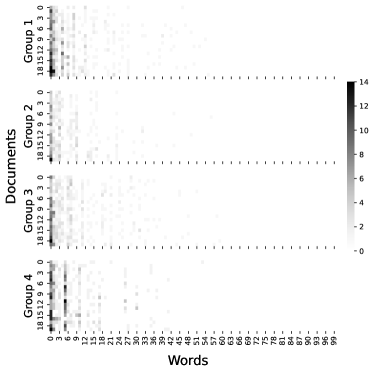
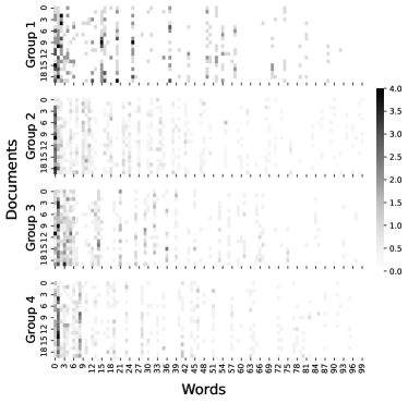
Figure 1: Word count matrices generated from GG-GG-Poisson HIBP model with parameters $J=4$, $\theta_{0}=10,\zeta=1$, $M_{j}=20$, $\theta_{j}\sim\mathrm{Unif}(2,4)$, $\alpha_{j}\sim\mathrm{Unif}(0.2,0.5)$, $\zeta_{j}=1$, and $\beta_{j}=1$ for $j\in[J]$. Left one is generated from $\alpha=0.2$ and right one is generated from $\alpha=0.7$. Showing top 100 words only.

4.2 Posterior Inference

Given a set of observed documents $\mathbf{Z}_{J}=((Z_{j}^{(i)},i\in[M_{j}]),j\in[J])$, one might be interested in inferring the parameters $\phi:=(\alpha,\zeta,\theta_{0},((\alpha_{j},\zeta_{j},\theta_{j},\beta_{j}),j\in[J]))$. In an ideal situation, the set of documents would contain all the counts, including $\xi(\varphi)=r$, $((X_{j,k}=n_{j,k},j\in[J]),k\in[r])$, and $((((\hat{A}^{(i)}_{j,k,l}=m_{j,k,l}^{(i)},i\in[M_{j}]),l\in[n_{j,k}]),j\in[J]),k\in[r])$. However, in practice, given a document, what we often observe is the total number of occurrences of word $k$ in document $i$ of group $j$; that is, $m_{j,k}^{(i)}:=\sum_{l=1}^{n_{j,k}}m_{j,k,l}^{(i)}$. In other words, we only observe the aggregated counts $m_{j,k}^{(i)}$ instead of observing the separated counts $m_{j,k,l}^{(i)}$ and the number of the separated counts $n_{j,k}$. To address this, in Section E.2, we derive a marginal likelihood of the word count matrices represented by the aggregated counts, $\mathbb{P}\Big{(}\xi(\varphi)=r,(\tilde{Y}_{k}\in dy_{k}),((X_{j,k}=n_{j,k})),(((\hat{A}_{j,k}=m_{j,k})))\Big{)}$, where $\hat{A}_{j,k}:=\sum_{i=1}^{M_{j}}\sum_{l=1}^{X_{j,k}}\hat{A}_{j,k,l}^{(i)}$, and present a posterior inference algorithm based on that. Note that we should still infer the counts $((X_{j,k}))$, which can be done via Gibbs sampling as we derive in Section E.3.

For demonstration, we generate documents $\mathbf{Z}_{J}$ with $\theta_{0}=10,\zeta=1,J=4,M_{j}=200,\theta_{j}\sim\mathrm{Unif}(2.0,4.0),\alpha_{j}\sim\mathrm{Unif}(0.1,0.6),\zeta_{j}=1,\beta_{j}=1$ for $j\in[J]$, and varying $\alpha$ values. We fix $\zeta,((\zeta_{j},\beta_{j}),j\in[J])$ to one, and inferred $\theta_{0},\alpha,((\theta_{j},\alpha_{j}),j\in[J])$ with the algorithm presented in Section E.2. We first test two configurations, one with $\alpha=0.2$ and another with $\alpha=0.6$. For each configuration, we run three independent chains with each chain run for 30,000 steps with 15,000 burn-in samples. Figure 2 presents posterior samples for $\theta_{0}$ and $\alpha$. The results for the remaining parameters are shown in Section E.3 in the supplementary material.

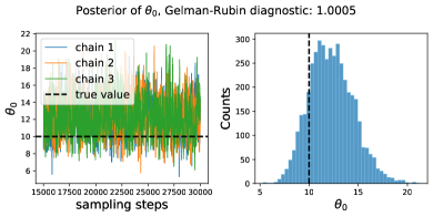
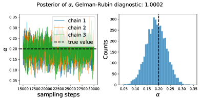
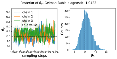
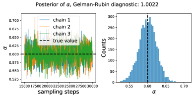
Figure 2: Posterior samples for $\theta_{0}$ and $\alpha$. Top row shows the results for the data generated with $\alpha=0.2$ and bottom row shows the ones with $\alpha=0.6$. We present Gelman-Rubin convergence diagnostic [9, 17]; Gelman-Rubin diagnostic values are clearly smaller than 1.2, indicating convergences.

4.3 Prediction and Classification

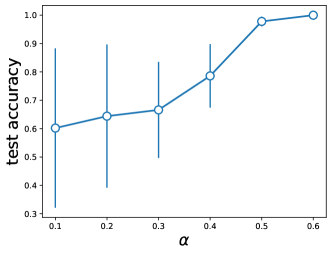
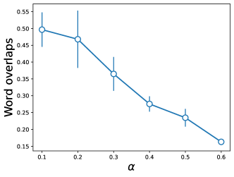
Figure 3: Left: average group classification accuracies for test documents generated with varying $\alpha$ values. Right: average overlap of words (see the main text for definition) across groups for the data generated with varying $\alpha$ values.

We further demonstrate that we can use our model for classifying documents by their groups. Given a set of documents $((Z_{j}^{(i)},i\in[M_{j}]),j\in[J])$, one can simulate or compute predictive probabilities of future documents using Theorem 3. Given a new document $Z_{*}$, for each $j\in[J]$, we compute the probability that $Z_{*}$ was generated from group $j$, $\mathbb{P}(Z_{*}=Z_{j}^{(M_{j}+1)}|\mathbf{Z}_{J})$. Then we can classify $Z_{*}$ to be in group $\arg\max_{j}\mathbb{P}(Z_{*}=Z_{j}^{(M_{j}+1)}|\mathbf{Z}_{J})$.

As an illustration, we generate training documents $\mathbf{Z}_{J}$ as described in Section 4.2, and further generate $100$ test documents per each group, using the prediction rule described in Theorem 3. See Section E.4 for the detailed description for the prediction process for GG-GG-Poisson HIBP case. We then run the posterior inference algorithm for the training data, collect the posterior samples, and compute the predictive probabilities of each test document belonging to one of $J$ groups. Here, similar to training, computing the predictive probabilities also requires working with the aggregated counts. In Section E.5, we present an algorithm to compute predictive probabilities when only the aggregated counts are observed.

Setting the parameters as in Section 4.2, we generate $\mathbf{Z}_{J}$ with $\alpha\in\{0.1,0.2,0.3,0.4,0.5,0.6\}$. For each $\alpha$ we generate five datasets, constituting 30 datasets in total. (Figure 3, left) summarizes the average test group classification accuracies w.r.t. $\alpha$ values used to generate data. We see that documents generated with larger $\alpha$ values are easier to classify; this is presumably because documents generated with larger $\alpha$ values are less likely to share words across groups. To see this, we measure the average overlap of words across groups,

$$\mathrm{Overlap}(\mathbf{Z}_{J}\,|\,\xi(\varphi)=r,((X_{j,k}=n_{j,k})))=\frac{1}{\binom{J}{2}}\sum_{j=1}^{J-1}\sum_{j^{\prime}=j+1}^{J}\sum_{k=1}^{r}\frac{\mathds{1}_{\{n_{j,k}>0\,\wedge\,n_{j^{\prime},k}>0\}}}{r},$$

that is, average portion of words co-occurring between all pairs of groups. (Figure 3, right) presents the $\mathrm{Overlap}(\mathbf{Z}_{J})$ values averaged across 5 datasets per each $\alpha$. As $\alpha$ increases, the average overlap decreases, indicating that documents from different groups become easier to distinguish.

Appendix A Proofs

In sections A.1-A.6 we provide details of the proofs, and related results, for the general HIBP model

Baseline $$B_{0} \sim\mathrm{CRM}(\tau_{0},G_{0})$$ (A.1)

Categories $$\mu_{j} \sim\mathrm{CRM}(\rho_{j},B_{0}) j\in[J]$$

Documents $$Z^{(i)}_{j} :=\sum_{l=1}^{\infty}A^{(i)}_{j,l}\delta_{\omega_{j,l}} i\in[M_{j}]$$

and, we provide corresponding details in sections A.7-A.10 for results in the general HHIBP model,

Baseline $$B_{0} \sim\mathrm{CRM}(\tau_{0},G_{0})$$ (A.2)

Categories $$B_{j} \sim\mathrm{CRM}(\tau_{j},B_{0}) j\in[J]$$

Subcategories $$\mu_{{d,j}} \sim\mathrm{CRM}(\rho_{d,j},B_{j}) d\in[D_{j}]$$

Documents $$Z^{(i)}_{d,j} :=\sum_{l=1}^{\infty}A^{(i)}_{d,j,l}\delta_{\omega_{d,j,l}} i\in[M_{d,j}]$$

A.1 Preliminary representations

We first describe other representations for $\mathbf{Z}_{J}:=((Z^{(i)}_{j},i\in[M_{j}),j\in[J])|B_{0},$ following the general HIBP (1.6). Recall that, conditional on $B_{0}$ these processes for each $j$ are specified by the mean measure $\prod_{i=1}^{M_{j}}G_{A_{j}}(da^{(i)}_{j}|s_{j})\rho_{j}(s_{j})B_{0}(d\omega).$ Hence using $B_{0}:=\sum_{k=1}^{\infty}\lambda_{k}\delta_{Y_{k}},$ the mean measure can be further expressed in terms of a countable sum of mean measures with components, $\prod_{i=1}^{M_{j}}G_{A_{j}}(da^{(i)}_{j}|s_{j})\rho_{j}(s_{j})\lambda_{k}\delta_{Y_{k}}(d\omega),$ for $k=1,2,\ldots.$ As can be verified by evaluating joint Laplace functionals, it follows that, conditional on $B_{0}$,

$$Z^{(i)}_{j}\overset{d}{=}\sum_{k=1}^{\infty}\left[\sum_{l=1}^{\infty}A^{(i)}_{j,k,l}\right]\delta_{Y_{k}}$$

where $A^{(i)}_{j,k,l}|s_{j,k,l}$ has distribution $G_{A_{j}}(da|s_{j,k,l})$ and for fixed $(j,k,l)$ are conditionally iid for $i\in[M_{j}],$ and independent across $(j,k,l)$ For each $(j,k),$ $\mathbf{s}_{j,k}=(s_{j,k,l},l=1,2,\ldots)$ are points of a PRM specified by the Lévy density $\rho_{j}(s)\lambda_{k},$ such that $\sum_{l=1}^{\infty}s_{j,k,l}\overset{d}{=}\sigma_{j,k}(\lambda_{k}),$ where for each $j$ $(\sigma_{j,k})\overset{iid}{\sim}\mathrm{CRM}(\rho_{j},\mathbb{L})$. That is,

$$\mathbb{E}[{\mbox{e}}^{-\kappa\sum_{l=1}^{\infty}s_{j,k,l}}|\lambda_{k}]=\mathbb{E}[{\mbox{e}}^{-\kappa\sigma_{j,k}(\lambda_{k})}|\lambda_{k}]={\mbox{e}}^{-\lambda_{k}\tilde{\psi}_{j}(\kappa)}.$$

Furthermore, for clarity, given $B_{0}$ the joint Laplace functional of $(\mu_{j}(f_{j}),j\in[J])$ for each $f_{j},$ a non-negative measurable function over $\Omega,$ can be expressed as

$$\mathbb{E}[{\mbox{e}}^{-\sum_{j=1}^{J}\mu_{j}(f_{j})}|B_{0}]=\prod_{j=1}^{J}\exp(-\int_{\Omega}\tilde{\psi}_{j}(f_{j}(\omega))B_{0}(d\omega))$$

which by expanding $B_{0}=\sum_{k=1}^{\infty}\lambda_{k}\delta_{Y_{k}},$ is equivalent to

$$\mathbb{E}[{\mbox{e}}^{-\sum_{j=1}^{J}\mu_{j}(f_{j})}|B_{0}]=\prod_{k=1}^{\infty}{\mbox{e}}^{-\lambda_{k}\sum_{j=1}^{J}\tilde{\psi}_{j}(f_{j}(Y_{k}))}$$

yielding, both conditional on $B_{0}$ and unconditonally,

$$(\mu_{j},j\in[J])\overset{d}{=}(\sum_{k=1}^{\infty}\sigma_{j,k}(\lambda_{k})\delta_{Y_{k}},j\in[J]),$$

which, as we mentioned in the main text, is known in the Lévy process literature, and will have specific utility in our setting.

As examples, if $Z^{(i)}_{j}|\mu_{j},B_{0}\sim\mathrm{BeP}(\mu_{j}),$ then $A^{(i)}_{j,k,l}\overset{d}{=}\mathscr{B}^{(i)}_{j,k,l}(s_{j,k,l}),$ that is $A^{(i)}_{j,k,l}|s_{j,k,l}\sim\mathrm{Bernoulli}(s_{j,k,l}),$ and hence

$$Z^{(i)}_{j}\overset{d}{=}\sum_{k=1}^{\infty}\left[\sum_{l=1}^{\infty}\mathscr{B}^{(i)}_{j,k,l}(s_{j,k,l})\right]\delta_{Y_{k}}$$ (A.3)

One can show that $\sum_{l=1}^{\infty}\mathscr{B}^{(i)}_{j,k,l}(s_{j,k,l})|B_{0}$ is $\mathrm{Poisson}(\lambda_{k}\int_{0}^{1}p\rho_{j}(p)dp),$ however the joint distribution of $(\sum_{l=1}^{\infty}\mathscr{B}^{(i)}_{j,k,l}(s_{j,k,l}),i\in[M_{j}])|B_{0}$ is not a vector of Poisson variables.

However, when $Z^{(i)}_{j}|\mu_{j},B_{0}\sim\mathrm{PoiP}(\kappa_{j},\mu_{j}),$ for each $j\in[J],$ it follows that $A^{(i)}_{j,k,l}\overset{d}{=}\mathscr{P}_{j,k,l}(\kappa_{j}s_{j,k,l})$, hence $\sum_{l=1}^{\infty}A^{(i)}_{j,k,l}\overset{d}{=}\mathscr{P}^{(i)}_{j,k}(\kappa_{j}\sum_{l=1}^{\infty}s_{j,k,l})\overset{d}{=}\mathscr{P}^{(i)}_{j,k}(\kappa_{j}\sigma_{j,k}(\lambda_{k})).$ Hence for the Poisson type HIBP it follows that the joint distribution of $((Z^{(i)}_{j},i\in[M_{j}),j\in[J])$ may be represented as

$$\left(\left(\sum_{k=1}^{\infty}\mathscr{P}^{(i)}_{j,k}(\kappa_{j}\sigma_{j,k}(\lambda_{k}))\delta_{Y_{k}},i\in[M_{j}]\right),j\in[J]\right)$$ (A.4)

which notably is a collection of mixed-Poisson processes, similar to what is encountered in (3.4), appearing in Proposition (3.1) and Proposition (3.2) in the HHIBP setting. See [30] for more on mixed-Poisson variables.

The representation in (A.4), while revealing an important structural form for the Poisson HIBP case, in terms of mixed Poisson processes, is deceptive in that it may seem that this particular representation is easiest to obtain pertinent analytic results. In fact, one may view the process as a multivariate type IBP, albeit a complex one, as in [27, Section 5]. Following [27, Section 5.1] take $I_{0}|\lambda$ to be equivalent in distribution to $((\mathscr{P}^{(i)}_{j}(\kappa_{j}\sigma_{j}(\lambda)),i\in[M_{j}]),j\in[J]),$ having the joint distribution

$$\mathbb{P}_{I_{0}}((I^{(i)}_{j}=m^{(i)}_{j},i\in[M_{j}],j\in[J])|\lambda)=\prod_{j=1}^{J}\frac{1}{\prod_{i=1}^{M_{j}}m^{(i)}_{j}!}\times\int_{0}^{\infty}x^{m_{j}}_{j}\kappa^{m_{j}}_{j}{\mbox{e}}^{-x_{j}\kappa_{j}M_{j}}F_{j}(dx_{j}|\lambda)$$

where $m_{j}:=\sum_{i=1}^{M_{j}}m^{(i)}_{j}$ and $\mathbb{P}(\sigma_{j}(\lambda)\in dx)=F_{j}(dx|\lambda).$ Hence the spike is

$$\mathbb{P}_{I_{0}}(\mathbf{0}|\lambda)=1-\pi_{I_{0}}(\lambda)=\prod_{j=1}^{J}\int_{0}^{\infty}{\mbox{e}}^{-x_{j}\kappa_{j}M_{j}}F_{j}(dx_{j}|\lambda)={\mbox{e}}^{-\lambda\sum_{j=1}^{J}\tilde{\psi}_{j}(\kappa_{j}M_{j})}.$$

This identifies the relevant multivariate spike and slab components, which are further mixed with respect to $\tau_{0}(\lambda).$ One may also work with $I_{0}|x_{1},\ldots,x_{J}$ with respect to the joint Lévy density $\rho_{J}(x_{1},\ldots,x_{J})dx_{1}\cdots dx_{J}=\int_{0}^{\infty}\prod_{j=1}^{J}F_{j}(dx_{j}|\lambda)\tau_{0}(d\lambda).$ Using either representation, applications of  [27, eqs. 51-52, and Propositions 5.1,5.2], almost immediately yield results parallel to (H1-H6). However the resulting forms would involve complex integrals with no obvious simple analytic form. To further illustrate this, suppose that $\mu_{j}|B_{0}$ are Gamma processes each specified by Lévy densities $\rho_{j}(s)=\theta_{j}s^{-1}{\mbox{e}}^{-s\zeta_{j}},$ for $j\in[J].$ Then it follows that $\sigma_{j}(\lambda)\sim\mathrm{Gamma}(\theta_{j}\lambda,\zeta_{j}),$ and we have $I_{0}:=((I^{(i)}_{j},i\in[M_{j}]),j\in[J])|\lambda$ has distribution,

$$\prod_{j=1}^{J}\frac{m_{j}!}{M^{m_{j}}_{j}\prod_{i=1}^{M_{j}}m^{(i)}_{j}!}\times{m_{j}+\theta_{j}\lambda-1\choose m_{j}}(1-p_{j})^{\theta_{j}\lambda}p^{m_{j}}_{j}$$ (A.5)

where $p_{j}=\kappa_{j}M_{j}/(\kappa_{j}M_{j}+\zeta_{j}).$

Treatment of cases such as the Bernoulli HIBP represented by (A.3), involves further delicate arguments. These points help to highlight the subtle aspects of the approach we develop, in terms of alternative representations, to achieve desirable forms of (H1-H6) for general choices of $(A_{j},j\in[J]).$

Remark A.1.

It is worthwhile to note that (A.5), for fixed $(M_{j},j\in[J]),$ correspond to Negative-Binomial type processes as discussed in [48, 50]. More specifically their gamma Negative Binomial processes arise when additionally $(\lambda_{k})$ are the jumps of a gamma process, that is $\tau_{0}(\lambda)=\theta_{0}\lambda^{-1}{\mbox{e}}^{\lambda\zeta}.$ The difficulties of using the direct representations are discussed in detail in [48, 50], and otherwise are clear from examining (A.5). Their solution is to use augmentations based on the Compound Poisson representation of Negative Binomial distributions due to [39]. Our developments have similarities, except that the number of cases where Compound Poisson representations for general mixed Poisson variables are known in the literature are very limited. We do not rely on this, but rather develop them based on results in [27].

A.2 Proofs of Propositions 2.1 and 2.2

We first establish Proposition 2.1. The idea, which is novel, is to view $\mathbf{Z}_{J}:=((Z^{(i)}_{j},i\in[M_{j}]),j\in[J])|B_{0}$ in terms of multivariate IBP processes using the framework of [27, Section 5]. For each $j\in[J],$ there is the vector $A_{0,j}:=(A^{(i)}_{j},i\in[M_{j}])|s$ with joint distribution $G_{A_{0,j}}(d\mathbf{a}_{j}|s):=\prod_{i=1}^{M_{j}}G_{A_{j}}(da^{(i)}_{j}|s),$ where $\mathbf{a}_{j}=(a^{(1)}_{j},\ldots,a^{(M_{j})}_{j}),$ are the possible values of $A_{0,j}.$ Restricting the arguments to $\mathbf{a}_{j}\notin\mathbf{0},$ meaning at least one of the components is non-zero, leads to a corresponding multivariate slab distribution

$$\frac{\mathbb{I}_{\{\mathbf{a}_{j}\notin\mathbf{0}\}}\prod_{i=1}^{M_{j}}G_{A_{j}}(da^{(i)}_{j}|s)}{(1-{[1-\pi_{A_{j}}(s)]}^{M_{j}})}$$ (A.6)

where $\mathbb{P}(A^{(1)}_{j}=0,\ldots,A^{(M_{j})}_{j}=0|s)={[1-\pi_{A_{j}}(s)]}^{M_{j}}:=1-\pi_{A_{0,j}}(s)$ is the corresponding spike. Now mixing with respect to the Lévy density $\rho_{j},$ leads to a random vector $(\hat{A}^{(1)}_{j},\ldots,\hat{A}^{(M_{j})}_{j})=(\hat{A}^{(1)}_{j},i\in[M_{j}])$ with a mixed multivariate truncated distribution

$$\mathsf{S}_{j}(a^{(1)}_{j},\ldots,a^{(M_{j})}_{j}|\rho_{j}):=\mathsf{S}_{j}(\mathbf{a}_{j}|\rho_{j})=\frac{\int_{0}^{\infty}\left[\prod_{i=1}^{M_{j}}G_{A_{j}}(da^{(i)}_{j}|s)\right]\rho_{j}(s)ds}{\psi_{j}(M_{j})}\mathbb{I}_{\{\mathbf{a}_{j}\notin\mathbf{0}\}}.$$ (A.7)

Equivalenty, there exists a variable $\tilde{H}_{j},$ with density $(1-{[1-\pi_{A_{j}}(s)]}^{M_{j}})\rho_{j}(s)/\psi_{j}(M_{j}),$ such that $(\hat{A}^{(i)}_{j},i\in[M_{j}])|\tilde{H}_{j}=s$ has joint distribution in (A.6).

Using [27, Proposition 5.2] with $A_{0,j}$ in place of $A_{0},$ leads to an initial representation of each $(Z^{(i)}_{j},i\in[M_{j}])|B_{0}$ for $j\in[J],$ with distribution denoted as $\mathrm{IBP}(A_{0,j},\rho_{j}B_{0}),$ note in our case $\rho_{j}$ is a univariate Lévy density. For clarity, this means the law of each vector $(Z^{(i)}_{j},i\in[M_{j}])|B_{0}$ is determined by the joint Laplace functional

$$\mathbb{E}[{\mbox{e}}^{-\sum_{i=1}^{M_{j}}t_{i}Z^{(i)}_{j}(f)}|B_{0}]=\exp(-\psi_{j}(M_{j})\int_{\mathbb{A}_{0,j}\times\Omega}(1-{\mbox{e}}^{-\sum_{i=1}^{M_{j}}t_{i}a^{(i)}_{j}f(\omega)})\mathsf{S}_{j}(\mathbf{a}_{j}|\rho_{j})B_{0}(d\omega))$$

where $\mathbb{A}_{0,j}$ is the support of $\mathbf{S}_{j}(\mathbf{a}_{j}|\rho_{j}),$ and $Z^{(i)}_{j}(f)=\sum_{l=1}^{\infty}A^{(i)}_{j,l}f(\omega_{j,l}),$ for some function $f$ over $\Omega.$ That is $(Z^{(i)}_{j},i\in[M_{j}])|B_{0}\sim\mathrm{IBP}(A_{0,j},\rho_{j}B_{0})$ means it is equivalent in distribution to the vector of compound Poisson processes $(\sum_{\ell=1}^{\xi_{j}}\hat{A}^{(i)}_{j,\ell}\delta_{\omega_{j,\ell}},i\in[M_{j}]),$ which are conditionally independent over $j\in[J],$ and where, $(\xi_{j},j\in[J])\overset{d}{=}(\mathscr{P}_{j}(\psi_{j}(M_{j})B_{0}(\Omega)),j\in[J]),$ independent of $((\omega_{j,\ell}),j\in[J])\overset{iid}{\sim}\bar{B}_{0},$ and $(\hat{A}^{(i)}_{j,\ell},i\in[M_{j}])\sim\mathsf{S}_{j}(\mathbf{a}_{j}|\rho_{j})$ independent across $(j,\ell).$ That is,

$$\left(\xi_{j},j\in[J]\right)|B_{0} \overset{d}{=}\quad\left(\mathscr{P}_{j}(\psi_{j}(M_{j})B_{0}(\Omega)),j\in[J]\right)$$ (A.8)

$$\left((\omega_{j,\ell}),j\in[J]\right)|B_{0} \overset{iid}{\sim}\quad\bar{B}_{0}$$

$$\left(\hat{A}^{(i)}_{j,\ell},i\in[M_{j}]\right) \sim\quad\mathsf{S}_{j}(\mathbf{a}_{j}|\rho_{j})$$

Hereafter we will not write out explicitly the Laplace functional and simply note that the law of each vector $(Z^{(i)}_{j},i\in[M_{j}])|B_{0}$ is determined by the Poisson mean measure $\psi_{j}(M_{j})\mathsf{S}_{j}(\mathbf{a}_{j}|\rho_{j})B_{0}(d\omega).$ Expanding $B_{0}=\sum_{k=1}^{\infty}\lambda_{k}\delta_{Y_{k}},$ leads to the countable collection of mean measures

$$\lambda_{k}\psi_{j}(M_{j})\mathsf{S}_{j}(\mathbf{a}_{j}|\rho_{j})\delta_{Y_{k}}(d\omega),$$

for $k=1,2,\ldots.$ Using these two forms of the mean measure. yields Proposition 2.1, in particular there are the following equivalent representations for $\mathbf{Z}_{J}|B_{0},$

$$\left(\left(\sum_{k=1}^{\infty}\left[\sum_{l=1}^{N_{j,k}}\hat{A}^{(i)}_{j,k,l}\right]\delta_{Y_{k}},i\in[M_{j}]\right),j\in[J]\right)\overset{d}{=}\left(\left(\sum_{\ell=1}^{\xi_{j}}\hat{A}^{(i)}_{j,\ell}\delta_{\omega_{j,\ell}},i\in[M_{j}]\right),j\in[J]\right)$$ (A.9)

where $((N_{j,k}),j\in[J])\overset{d}{=}((\mathscr{P}_{j,k}(\lambda_{k}\psi_{j}(M_{j})),j\in[J]).$

For the process $(\sum_{k=1}^{\infty}N_{j,k}\delta_{Y_{k}},j\in[J])$ in Proposition 2.2, we may treat it as a single realization of multivariate IBP of vector length $J,$ with $N_{0}:=(N_{1},\ldots,N_{J})$ playing the role of $A_{0}$ in [27, Section 5], where $N_{0}|\lambda$ has distribution $\prod_{j=1}^{J}\lambda^{m_{j}}\psi_{j}^{m_{j}}(M_{j}){\mbox{e}}^{-\lambda\psi_{j}(M_{j})}/m_{j}!,$ corresponding to a product of $J$ independent Poisson variables with parameters $(\lambda\psi_{j}(M_{j}),j\in[J]).$ It follows that the multivariate slab distribution is $N^{\prime}_{0}|\lambda\sim\mathrm{tPoisson}(\lambda\psi_{1}(M_{1}),\ldots,\lambda\psi_{J}(M_{J})),$ as described in [46, Section 4.1.1, p. 501], the corresponding spike is $1-\pi_{N_{0}}(\lambda)={\mbox{e}}^{-\lambda\sum_{j=1}^{J}\psi_{j}(M_{j})}.$ Using these points, the representation in Proposition 2.2 corresponds to a process with an $\mathrm{IBP}(N_{0},\tau_{0}G_{0})$ distribution as described in [27, Proposition 5.2]. That it is to say we have proven that

$$\left(\sum_{k=1}^{\infty}N_{j,k}\delta_{Y_{k}},j\in[J]\right)\overset{d}{=}\left(\sum_{k=1}^{\xi(\varphi)}X_{j,k}\delta_{\tilde{Y}_{k}},j\in[J]\right)$$ (A.10)

where $X_{0,k}:=(X_{1,k},\ldots X_{J,k})\sim\mathrm{MtP}((\psi_{j}(M_{j}),j\in[J]),\tau_{0}).$ We now provide more details on the class of $\mathrm{MtP}$ distributions.

Definition A.1.

Let $(V_{0}=(V_{1},\ldots,V_{J}))$ denote a random vector and consider the pair of variables $(V_{0},H_{0}).$ We say that $V_{0}$ has a multivariate mixed zero-truncated Poisson distribution of vector length $J$ with non-negative parameters $(\kappa_{j},j\in[J])$ and Lévy density $\tau_{0},$ and write $V_{0}\sim\mathrm{MtP}((\kappa_{j},j\in[J]),\tau_{0}),$ if $(V_{0},H_{0})$ satisfies the following properties for $\kappa=\sum_{j=1}^{J}\kappa_{j}$ and $\pi_{j}=\kappa_{j}/\kappa.$

1. $V_{0}|H_{0}=\lambda\sim\mathrm{tPoisson}(\lambda\kappa_{1},\ldots,\lambda\kappa_{J}),$ has the joint probability mass function, with non-negative integer arguments $(m_{1},\ldots,m_{J}),$ such that $m:=\sum_{j=1}^{J}m_{j}\in\{1,2,\ldots\},$

   $$\frac{m!}{\prod_{j=1}^{J}m_{j}!}\prod_{j=1}^{J}\pi^{m_{j}}_{j}\times\frac{{(\kappa\lambda)}^{m}{\mbox{e}}^{-\kappa\lambda}}{m!(1-{\mbox{e}}^{-\lambda\kappa})}$$ (A.11)

2. $\tilde{V}:=\sum_{j=1}^{J}V_{j}|H_{0}=\lambda$ has zero-truncated $\mathrm{Poisson}(\lambda\kappa)$ distribution with law denoted as $\mathrm{tPoisson}(\lambda\kappa)$ and $H_{0}$ has density

   $$\mathbb{P}_{H_{0}}(d\lambda)/d\lambda=\frac{(1-{\mbox{e}}^{-\lambda\kappa})\tau_{0}(\lambda)}{\tilde{\psi}_{0}(\kappa)}$$ (A.12)

3. $V_{0}|\tilde{V}=m$ is $\mathrm{Multinomial}(m,(\pi_{j},j\in J))$

4. Furthermore $\tilde{V}:=\sum_{j=1}^{J}V_{j}\sim\mathrm{MtP}(\kappa,\tau_{0}),$ has the probability mass function for $m=1,2,\ldots,$

   $$\tilde{p}(m|\kappa,\tau_{0})=\frac{\kappa^{m}\int_{0}^{\infty}\lambda^{m}{\mbox{e}}^{-\lambda\kappa}\tau_{0}(\lambda)d\lambda}{m!\tilde{\psi}_{0}(\kappa)}$$ (A.13)

5. The joint probability mass function of $V_{0}=(V_{1},\ldots,V_{J}),$ has the form

   $$\tilde{p}(m_{1},\ldots,m_{J}|(\kappa_{j},j\in[J]),\tau_{0})=\frac{m!}{\prod_{j=1}^{J}m_{j}!}\prod_{j=1}^{J}\pi^{m_{j}}_{j}\times\tilde{p}(m|\kappa,\tau_{0})$$ (A.14)

Remark A.2.

The mean measure that specifies the $\mathrm{IBP}(N_{0},\tau_{0}G_{0})$ distributed process in (A.10) can be expressed as

$$\tilde{\psi}_{0}\left(\sum_{j=1}^{J}\psi_{j}(M_{j})\right)\tilde{p}\left(m_{1},\ldots,m_{J}|(\psi_{j}(M_{j}),j\in[J]),\tau_{0}\right)G_{0}(dy)$$

A.3 Proof of Theorem 1

In principle, the result can be obtained by using Proposition 2.1 and Proposition 2.2 along with a special application of [27, Proposition 5.2], however there are some delicate details to note. The key is to identify the spike and slab distributional decomposition of the components in Proposition 2.1, which is not immediately obvious. In particular, a direct approach using [27, Proposition 5.2] seems to suggest that a closed form expression for the joint density of the relevant slab distribution is required. However that expression would be quite complex, and not immediately indicative of the representations we obtain. We proceed by first identifying the spike distribution. This is done by noting that for each $k,$ the vector

$$\left(\left(\sum_{l=1}^{N_{j,k}}\hat{A}^{(i)}_{j,k,l},i\in[M_{j}]\right),j\in[J]\right),$$ (A.15)

appearing in Proposition 2.1, has all components equal to zero if and only if $N_{j,k}=0$ for $j\in[J].$ Hence the spike distribution for constructing $((Z^{(i)}_{j},i\in[M_{j}]),j\in[J])$ is the same as that for $(\sum_{k=1}^{\infty}N_{j,k}\delta_{Y_{k}},j\in[J]).$ The requisite slab distribution can then be expressed as the distribution of the vector in (A.15) conditioned on the complement of the event $(N_{j,k}=0,j\in[J]).$ The result is then completed by utilizing the results, and details in the proof of Proposition 2.1 and Proposition 2.2.

A.4 Descriptions of HIBP joint marginal distributions

Due to space considerations we have omitted descriptions of the relevant joint distributions of $\mathbf{Z}_{J}:=((Z^{(i)}_{j},i\in[M_{j}]),j\in[J]),$ in the main text. That is to say the unconditional joint (marginal) distribution of $\mathbf{Z}_{J}$ obtained by taking expectations with respect to $(\mu_{j},j\in[J]),B_{0}.$ We now provide details. The approach is not to use the multivariate framework in [27, Section 5], but rather first to apply results, perhaps more familiar to some readers, appearing in [27, Proposition 3.1]. Assume that $(\xi_{j}=v_{j},j\in[J]),$ for $v_{j}=0,1,2,\ldots,$ appearing in (A.8). It is important to note that while the variables $(\omega_{j,\ell},\ell\in[v_{j}]),$ which are atoms of $\mu_{j}$ that are selected conditionally iid from the discrete distribution $\bar{B}_{0},$ may contain ties, the corresponding unobserved jumps of $\mu_{j},$ say $(S_{j,\ell},\ell\in[v_{j}]),$ are distinct. Hence the pairs $((S_{j,\ell},\omega_{j,\ell}),\ell\in[v_{j}])$ are distinct, for each $j\in[J].$ Applying, for each $j\in[J],$ [27, Proposition 3.1], the joint distribution of $(Z^{(i)}_{j},i\in[M_{j})|B_{0}$ can be expressed as

$$\left[\prod_{\ell=1}^{v_{j}}\mathsf{S}_{j}(\mathbf{a}_{j,\ell}|\rho_{j})\right]{[\psi_{j}(M_{j})]}^{v_{j}}{\mbox{e}}^{-\psi_{j}(M_{j})B_{0}(\Omega)}\prod_{\ell=1}^{v_{j}}B_{0}(d\omega_{j,\ell})$$ (A.16)

and the jumps $(S_{j,\ell},\ell\in[v_{j}])|(Z^{(i)}_{j},i\in[M_{j}]),B_{0},$ are conditionally independent with respective densities equivalent to,

$$\vartheta(s|\mathbf{a}_{j,\ell},\rho_{j})\propto\left[\prod_{i=1}^{M_{j}}G_{A_{j}}(da^{(i)}_{j,\ell}|s)\right]\rho_{j}(s).$$ (A.17)

Furthermore setting $\mathsf{S}_{j}(\mathbf{a}_{j}|\rho_{j})=1,$ for $j\in[J],$ it follows from (A.9) and (A.16) that the joint distribution of $(\sum_{k=1}^{\infty}N_{j,k}\delta_{Y_{k}},j\in[J])|B_{0}$ may be expressed as

$$\prod_{j=1}^{J}{[\psi_{j}(M_{j})]}^{v_{j}}{\mbox{e}}^{-\psi_{j}(M_{j})B_{0}(\Omega)}\prod_{\ell=1}^{v_{j}}B_{0}(d\omega_{j,\ell})$$ (A.18)

We assume that the realization of $\mathbf{Z}_{J}:=((Z^{(i)}_{j},i\in[M_{j}]),j\in[J])),$ based on the representation in Theorem 1

$$\mathbf{Z}_{J}:=\left(\left(Z^{(i)}_{j},i\in[M_{j}]\right),j\in[J]\right)\overset{d}{=}\left(\left(\sum_{k=1}^{\xi(\varphi)}\left[\sum_{l=1}^{X_{j,k}}\hat{A}^{(i)}_{j,k,l}\right]\delta_{\tilde{Y}_{k}},i\in[M_{j}]\right),j\in[J]\right),$$

has the following component values, $\xi({\varphi})=r,(({X}_{1,k}=n_{1,k},\ldots,{X}_{J,k}=n_{J,k}),k\in[r]),$ with $\sum_{j=1}^{J}n_{j,k}=n_{k},$ $(\hat{A}^{(i)}_{j,k,l},i\in[M_{j}])=\mathbf{a}_{j,k,l}:=(a^{(i)}_{j,k,l},i\in[M_{j}]).$ and $(\tilde{Y}_{k},k\in[r])$ observed features. In terms of the right hand side of (A.9), for $(\hat{A}^{(i)}_{j,\ell},i\in[M_{j}])=\mathbf{a}_{j,\ell}),$ there is the correspondence $(\mathbf{a}_{j,\ell},\ell\in[v_{j}])=(\mathbf{a}_{j,k,l},l\in[n_{j,k}],k\in[r]),$ where $v_{j}=\sum_{k=1}^{r}n_{j,k}$ and $n=\sum_{j=1}^{J}v_{j}=\sum_{k=1}^{r}n_{k}.$ Using slightly different notation than in [49, Corollary 2], including an extra parameter $\kappa=\sum_{j=1}^{J}\psi_{j}(M_{j})>0,$ for $\gamma_{0}:=G_{0}(\Omega),$ , and positive cell counts $\mathbf{n}_{r}:=(n_{1},\ldots,n_{r})$, where $\sum_{k=1}^{r}n_{k}=n,$ the marginal distribution of $\sum_{k=1}^{\infty}[\sum_{j=1}^{J}N_{j,k}]\delta_{Y_{k}}$ is equivalent to

$$n!\varrho(\mathbf{n}_{r};n|\gamma_{0},\tau_{0},\kappa)\times\prod_{k=1}^{r}\bar{G}_{0}(d\tilde{Y}_{k})$$

for

$$\varrho(\mathbf{n}_{r};n|\gamma_{0},\tau_{0},\kappa)=\frac{\gamma^{r}_{0}}{n!}{\mbox{e}}^{-\gamma_{0}\int_{0}^{\infty}(1-{\mbox{e}}^{-\lambda\kappa})\tau_{0}(\lambda)d\lambda}\prod_{k=1}^{r}n_{k}!\tilde{\psi}_{0}(\kappa)\tilde{p}(n_{k}|\kappa,\tau_{0}),$$ (A.19)

where $n_{k}!\tilde{\psi}_{0}(\kappa)\tilde{p}(n_{k}|\kappa,\tau_{0})=\int_{0}^{\infty}\kappa^{n_{k}}\lambda^{n_{k}}{\mbox{e}}^{-\lambda\kappa}\tau_{0}(\lambda)d\lambda.$ The function in (A.19) is an exchangeable cluster probability function ($\mathrm{ECPF}$) as discussed in [49].

Remark A.3.

See [29, Proposition 4 and eq. (5)], and also [4, Section 2.3], for other interpretations of the ECPF in (A.19). [38] provides additional interpretations, and points out these correspondences to earlier work of Fisher and McCloskey on species sampling models. See also [23].

Equivalently a description of the unconditional joint distribution (the joint marginal distribution) of $\mathbf{Z}_{J},$ is completed by evaluating

$$\mathbb{E}[{\mbox{e}}^{-B_{0}(\Omega)\sum_{j=1}^{J}\psi_{j}(M_{j})}\prod_{j=1}^{J}\prod_{\ell=1}^{v_{j}}B_{0}(d\omega_{j,\ell})],$$

which by [24, Propositions 2.1-2.2], is equivalent to

$${\mbox{e}}^{-G_{0}(\Omega)\tilde{\psi}_{0}(\sum_{j=1}^{J}\sum_{j=1}^{J}\psi_{j}(M_{j}))}\prod_{k=1}^{r}\int_{0}^{\infty}\lambda^{n_{k}}{\mbox{e}}^{-\lambda\sum_{j=1}^{J}\psi_{j}(M_{j})}\tau_{0}(\lambda)d\lambda\times G_{0}(d\tilde{Y}_{k}).$$

where $\sum_{k=1}^{r}n_{k}=\sum_{j=1}^{J}v_{j}:=n,$ with $\sum_{k=1}^{r}n_{j,k}=v_{j}.$ Now for $\kappa=\sum_{j=1}^{J}\psi_{j}(M_{j})$ and $\gamma_{0}=G_{0}(\Omega),$ set

$$\hat{\varrho}(\mathbf{n}_{r}|\gamma_{0},\tau_{0},\kappa):={\mbox{e}}^{-G_{0}(\Omega)\tilde{\psi}_{0}(\sum_{j=1}^{J}\sum_{j=1}^{J}\psi_{j}(M_{j}))}\prod_{k=1}^{r}\int_{0}^{\infty}\lambda^{n_{k}}{\mbox{e}}^{-\lambda\sum_{j=1}^{J}\psi_{j}(M_{j})}\tau_{0}(\lambda)d\lambda$$

Now, using the convention $\prod_{l=1}^{n_{j,k}}c_{l}=1$ for $n_{j,k}=0,$ we can write,

$$\mathbf{S}_{[J]}(\mathbf{a}):=\prod_{j=1}^{J}\left[\prod_{\ell=1}^{v_{j}}\mathsf{S}_{j}(\mathbf{a}_{j,\ell}|\rho_{j})\right]=\prod_{j=1}^{J}\prod_{k=1}^{r}\prod_{l=1}^{n_{j,k}}\mathsf{S}_{j}(\mathbf{a}_{j,k,l}|\rho_{j}),$$ (A.20)

which is the likelihood of

$$((\hat{A}^{(i)}_{j,\ell},i\in[M_{j}]),\ell\in[v_{j}],j\in[J])\overset{d}{=}(((\hat{A}^{(1)}_{j,k,l},\ldots,\hat{A}^{(M_{j})}_{j,k,l}),l\in[n_{j,k}],k\in[r]),j\in J),$$

otherwise the same as in the respective non-hierarchical cases.

The derivations above lead to the following description of the marginal joint distribution of $\mathbf{Z}_{D,J},$ which can otherwise be sampled according to Theorem 4.

Proposition A.1.

Set $\kappa=\sum_{j=1}^{J}\psi_{j}(M_{j})$, and $((X_{j,k}=n_{j,k},j\in[J],k\in[r]),\xi(\varphi)=r),$ $\sum_{j=1}^{J}n_{j,k}=n_{k}>0,$ $\sum_{k=1}^{r}n_{j,k}=v_{j}$ and $\sum_{j=1}^{J}v_{j}=n,$ and $(\hat{A}^{(i)}_{j,k,l},i\in[M_{j}])=\mathbf{a}_{j,k,l}.$ Then the marginal distribution of $((Z^{(i)}_{j},i\in[M_{j}]),j\in[J])$ can be expressed as,

$$\mathbf{S}_{[J]}(\mathbf{a})\times\prod_{j=1}^{J}\psi_{j}(M_{j})^{v_{j}}\times\hat{\varrho}(\mathbf{n}_{r}|\gamma_{0},\tau_{0},\kappa)\times\prod_{k=1}^{r}{G}_{0}(d\tilde{Y}_{k})$$ (A.21)

Remark A.4.

One may also express (A.21) in terms of the ECPF, since $n!\varrho(\mathbf{n}_{r};n|\gamma_{0},\tau_{0},\kappa)=\gamma^{r}_{0}\hat{\varrho}(\mathbf{n}_{r}|\gamma_{0},\tau_{0},\kappa)$. One consequence is this allows for an simple adaptation of the computational procedures outlined in [49].

A.4.1 Multi-group ECPF

As a Corollary, the next result, which may be compared with [49, Corollary 2], describes a multi-group version of an $\mathrm{ECPF}.$

Corollary A.1.

Set $\sum_{j=1}^{J}v_{j}=n,$ and let $K(n)=r\in[n]$ denote the number of distinct points $(\tilde{Y}_{1},\ldots,\tilde{Y}_{r})$ drawn from $n$ samples from $\bar{B}_{0}.$ Further note that $v_{j}=\sum_{k=1}^{r}n_{j,k},$ and $\sum_{k=1}^{r}n_{k}=\sum_{j=1}^{J}v_{j}=n.$

1. Then the joint distribution of random variables $(({\omega}_{j,\ell},\ell\in[\xi_{j}],\xi_{j}=v_{j}),j\in[J]),$ described in (A.8) can be expressed as

   $$\frac{n!\prod_{j=1}^{J}\pi^{v_{j}}_{j}}{\prod_{j=1}^{J}v_{j}!}\times\varrho(\mathbf{n}_{r};n|\gamma_{0},\tau_{0},\sum_{j=1}^{J}\psi_{j}(M_{j}))\times\prod_{k=1}^{r}\bar{G}_{0}(d\tilde{Y}_{k})$$ (A.22)

   where $\gamma_{0}=G_{0}(\Omega),$ and $[\sum_{k=1}^{J}\psi_{k}(M_{j})]\pi_{j}=\psi_{j}(M_{j})$ for $j=1,\ldots,J.$

2. The distribution of the variables in $[(i)],$ is equivalent to

   $$\frac{r!\prod_{k=1}^{r}\prod_{j=1}^{J}n_{j,k}!}{\prod_{j=1}^{J}v_{j}!}$$

   times the distribution of $((X_{j,k}=n_{j,k},j\in[J]),\tilde{Y}_{k}),k\in[\xi(\varphi)]),\xi(\varphi)=r).$

A.5 Proof of the HIBP posterior distributions in Theorem 2

We now provide the proof for the posterior distributions of $B_{0},(\mu_{j},j\in[J])|\mathbf{Z}_{J},$ as described in Theorem 2. It follows from (A.16) and (A.18) that the distribution of $B_{0}|\mathbf{Z}_{J}$ is the same as $B_{0}|(\sum_{k=1}^{\infty}N_{j,k}\delta_{Y_{k}},j\in[J]),$ and furthermore is equivalent to $B_{0}|\sum_{k=1}^{\infty}[\sum_{j=1}^{J}N_{j,k}]\delta_{Y_{k}},$ where

$$\sum_{k=1}^{\infty}\left[\sum_{j=1}^{J}N_{j,k}\right]\delta_{Y_{k}}|B_{0}\sim\mathrm{PoiP}\left(\sum_{j=1}^{J}\psi_{j}(M_{j}),B_{0}\right).$$

Hence the result, as described in Theorem 2, can be read from [27, See section 4.2], based on $M=1$ customer. That is $B_{0}|\mathbf{Z}_{J},$ has the representation

$$B_{0,J}+\sum_{k=1}^{r}\tilde{L}_{k}\delta_{\tilde{Y}_{k}},$$ (A.23)

where $B_{0,J}=\sum_{k=1}^{\infty}\lambda^{\prime}_{k}\delta_{Y^{\prime}_{k}}\sim\mathrm{CRM}(\tau_{0,J},G_{0}),$ independent of $(\tilde{L}_{k},k\in[r]).$ An application of [27, Theorem 3.1] shows that the posterior distribution of $\mu_{j}|\mathbf{Z}_{J},B_{0}$ is equivalent to

$$\hat{\mu}_{j,M_{j}}+\sum_{\ell=1}^{v_{j}}S_{j,\ell}\delta_{\omega_{j,\ell}}$$

where $\hat{\mu}_{j,M_{j}}|B_{0}$ is $\mathrm{CRM}(\rho^{(M_{j})}_{j},B_{0}).$ Now using the posterior representation of $B_{0}|\mathbf{Z}_{J},$ in (A.23), $\mathrm{CRM}(\rho^{(M_{j})}_{j},B_{0}),$ is equivalent to the sum of the CRMs, $\mathrm{CRM}(\rho^{(M_{j})}_{j},B_{0,J})$ and $\mathrm{CRM}(\rho^{(M_{j})}_{j},\sum_{k=1}^{r}\tilde{L}_{k}\delta_{\tilde{Y}_{k}}),$ and it follows that the distribution of $\hat{\mu}_{j,M_{j}}|\mathbf{Z}_{J}$ corresponds to that of $\tilde{\mu}_{j,M_{j}}+\sum_{k=1}^{r}\tilde{\sigma}_{j,k}(\tilde{L}_{k})\delta_{\tilde{Y}_{k}}.$ The result is concluded by noting that $((S_{j,\ell},\omega_{j,\ell}),\ell\in[v_{j}])\overset{d}{=}((S_{j,k,l},\tilde{Y_{k}}),l\in[n_{j,k}],k\in[r]),$ where $(\omega_{j,\ell}),(\tilde{Y}_{k})$ are fixed, hence

$$\sum_{\ell=1}^{v_{j}}S_{j,\ell}\delta_{\omega_{j,\ell}}\overset{d}{=}\sum_{k=1}^{r}\left[\sum_{\ell\in E_{j,k}}S_{j,\ell}\right]\delta_{\tilde{Y}_{k}}\overset{d}{=}\sum_{k=1}^{r}\left[\sum_{l=1}^{n_{j,k}}S_{j,k,l}\right]\delta_{\tilde{Y}_{k}},$$ (A.24)

where $E_{j,k}:=\{\ell:\omega_{j,\ell}=\tilde{Y}_{k}\}.$ That is $(\mu_{j},j\in[J))|\mathbf{Z}_{J}$ is equivalent in distribution to the vector of random measures

$$(\tilde{\mu}_{j,M_{j}}+\sum_{k=1}^{r}\tilde{\sigma}_{j,k}(\tilde{L}_{k})\delta_{\tilde{Y}_{k}}+\sum_{k=1}^{r}\left[\sum_{l=1}^{n_{j,k}}S_{j,k,l}\right]\delta_{\tilde{Y}_{k}},j\in[J])$$ (A.25)

for $\tilde{\mu}_{j,M_{j}}=\sum_{v=1}^{\infty}\tilde{\sigma}_{j,v+r}(\lambda^{\prime}_{v})\delta_{Y^{\prime}_{v}}|B_{0,J}\sim\mathrm{CRM}(\rho^{(M_{j})}_{j},B_{0,J})$, and $(\tilde{\sigma}_{j,k})\overset{iid}{\sim}\mathrm{CRM}(\rho^{(M_{j})}_{j},\mathbb{L})$ independent of $(\tilde{L}_{k}),$ and $(S_{j,k,l}).$

A.6 Proof of HIBP prediction rule in Theorem 3

Apply [27, Proposition 3.2] to obtain a description of the predictive distribution of ${Z}^{(M_{j}+1)}_{j}|\mathbf{Z}_{J},B_{0},$ equating to $\hat{Z}_{j}+\sum_{\ell=1}^{v_{j}}A_{j,\ell}\delta_{\omega_{j,\ell}},$ where due to notational suppression $A_{j,\ell}:=A^{(M_{j}+1)}_{j,\ell}.$ It follows that

$$\sum_{\ell=1}^{v_{j}}A_{j,\ell}\delta_{\omega_{j,\ell}}\overset{d}{=}\sum_{k=1}^{r}\left[\sum_{\ell\in E_{j,k}}A_{j,\ell}\right]\delta_{\tilde{Y}_{k}}\overset{d}{=}\sum_{k=1}^{r}\left[\sum_{l=1}^{n_{j,k}}A_{j,k,l}\right]\delta_{\tilde{Y}_{k}},$$

for $E_{j,k}:=\{\ell:\omega_{j,\ell}=\tilde{Y}_{k}\}$ and $\hat{Z}_{j}|\mathbf{Z}_{J},B_{0},$ has an $\mathrm{IBP}(A_{j},\rho^{(M_{j})}_{j}B_{0})$ distribution which means that it can be represented as a compound Poisson process based on the mean measure $\gamma^{(M_{j}+1)}_{j}\mathsf{S}_{j}(a|\rho^{(M_{j})}_{j})B_{0}(d\omega),$ where $\mathsf{S}_{j}(a|\rho^{(M_{j})}_{j})$ denotes the univariate distribution in (2.6). Use (A.23) to express the mean measure as

$$\gamma^{(M_{j}+1)}_{j}\mathsf{S}_{j}(a|\rho^{(M_{j})}_{j})({B}_{0,J}(d\omega)+\sum_{k=1}^{r}\tilde{L}_{k}\delta_{\tilde{Y}_{k}}(d\omega))$$

and hence $\hat{Z}_{j}|\mathbf{Z}_{J}$ as a sum of an $\mathrm{IBP}(A_{j},\rho^{(M_{j})}_{j}{B}_{0,J})$ and $\mathrm{IBP}(A_{j},\rho^{(M_{j})}_{j}\sum_{k=1}^{r}\tilde{L}_{k}\delta_{\tilde{Y}_{k}})$ process. Since ${B}_{0,J}=\sum_{k=1}^{\infty}\tau^{\prime}_{k}\delta_{Y^{\prime}_{k}}\sim\mathrm{CRM}(\tau_{0,J},G_{0}),$ the first term in (2.8) follows by applying Proposition 2.1 and Theorem 1, to the univariate $\mathrm{IBP}(A_{j},\rho^{(M_{j})}_{j}{B}_{0,J})$ with appropriate adjustments. The second term follows directly by expanding $\sum_{k=1}^{r}\tilde{L}_{k}\delta_{\tilde{Y}_{k}}.$

A.7 Proof of HHIBP Proposition 3.1, Proposition 3.2 and Theorem 4

Recall that given $B_{1}.\ldots,B_{J},B_{0},$ for each fixed $(d,j)$ $((A^{(i)}_{d,j,l},i\in[M_{d,j}]),s_{d,j,l},\omega_{d,j,l})),$ are points of a $\mathrm{PRM}$ with mean intensity $\prod_{i=1}^{M_{d,j}}G_{A_{d,j}}(da^{(i)}_{d,j}|s_{d,j})\rho_{d,j}(s_{d,j})B_{j}(d\omega).$ Hence, given $B_{1}.\ldots,B_{J},B_{0},$ for each $(d,j)$ this leads to a representation based on the mean measure

$$\psi_{d,j}(M_{d,j})\mathsf{S}_{d,j}(\mathbf{a}_{d,j}|\rho_{d,j})B_{j}(d\omega_{j}),$$ (A.26)

as in the HIBP case, with $j$ in place of $(d,j).$ Using the representation $B_{j}=\sum_{l=1}^{\infty}\lambda_{j,l}\delta_{w_{j,l}}$ creates the countable collection of mean measures

$$\lambda_{j,l}\psi_{d,j}(M_{d,j})\mathsf{S}_{d,j}(\mathbf{a}_{d,j}|\rho_{d,j})\delta_{w_{j,l}}(d\omega),$$

for $l=1,2,\ldots,$ leading to the following representation for each $j$, conditionally independent across $j\in[J],$ ,

$$\left(\left(\sum_{l=1}^{\infty}\left[\sum_{t=1}^{\tilde{N}_{d,j,l}}\hat{A}^{(i)}_{d,j,l,t}\right]\delta_{w_{j,l}},i\in[M_{d,j}]\right),d\in[D_{j}]\right)\overset{d}{=}\left(\left(\sum_{\ell=1}^{\xi_{d,j}}\hat{A}^{(i)}_{d,j,\ell}\delta_{\omega_{d,j,\ell}},i\in[M_{d,j}]\right),d\in[D_{j}]\right)$$ (A.27)

where $((\tilde{N}_{d,j,l}),d\in[D_{j}])\overset{d}{=}((\mathscr{P}_{d,j,l}(\lambda_{j,l}\psi_{d,j}(M_{d,j})),d\in[D_{j}]),$ and for the right-hand side of equation (A.27), given $B_{j},$ $(\xi_{d,j},d\in[D_{j}])\overset{d}{=}(\mathscr{P}_{d,j}(\psi_{d,j}(M_{d,j})B_{j}(\Omega)),d\in[D_{j}]),$ independent of $((\omega_{d,j,\ell}),d\in[D_{j}])\overset{iid}{\sim}\bar{B}_{j},$ and $(\hat{A}^{(i)}_{d,j,\ell},i\in[M_{d,j}])\sim\mathsf{S}_{d,j}(\mathbf{a}_{d,j}|\rho_{d,j})$ independent across $(d,j,\ell).$

Remark A.5.

Note furthermore we can define $\xi_{j}=\sum_{j=1}^{D_{j}}\xi_{d,j}\overset{d}{=}\mathscr{P}_{j}(B_{j}(\Omega)\sum_{d=1}^{D_{j}}\psi_{d,j}(M_{d,j}))$ and $\xi=\sum_{j=1}^{J}\xi_{j}\overset{d}{=}\mathscr{P}(\sum_{j=1}^{J}B_{j}(\Omega)\sum_{d=1}^{D_{j}}\psi_{d,j}(M_{d,j})).$

Now, instead, using the representation $(B_{1},\ldots,B_{J})\overset{d}{=}(\sum_{k=1}^{\infty}\varepsilon_{j,k}(\lambda_{k})\delta_{Y_{k}},j\in[J]),$ and expanding each $B_{j}$ in (A.26), leads to the countable collection of mean measures

$$\varepsilon_{j,k}(\lambda_{k})\psi_{d,j}(M_{d,j})\mathsf{S}_{d,j}(\mathbf{a}_{d,j}|\rho_{d,j})\delta_{Y_{k}}(d\omega),$$

for $k=1,2,\ldots,$ which shows that $\mathbf{Z}_{D,J}:=(((Z^{(i)}_{d,j},i\in[M_{d,j}]),j\in[D_{j}]),j\in[J])|B_{0},$ can be represented as

$$\left(\left(\left(\sum_{k=1}^{\infty}\left[\sum_{l=1}^{N_{d,j,k}}\hat{A}^{(i)}_{d,j,k,l}\right]\delta_{Y_{k}},i\in[M_{d,j}]\right),d\in[D_{j}]\right),j\in[J]\right)$$

where $(((N_{d,j,k}),d\in[D_{j}]),j\in[J])\overset{d}{=}(((\mathscr{P}_{d,j,k}(\psi_{d,j}(M_{d,j})\varepsilon_{j,k}(\lambda_{k})),d\in[D_{j}]),j\in[J]).$ as in Proposition 3.1

We now proceed to the proof of Proposition 3.2, which gives a tractable form to sample the joint distribution of

$$\left(\left(\sum_{k=1}^{\infty}\mathscr{P}_{d,j,k}(\psi_{d,j}(M_{d,j})\varepsilon_{j,k}(\lambda_{k}))\delta_{Y_{k}},d\in[D_{j}]\right),j\in[J]\right).$$ (A.28)

As we mentioned in the main text, we may view the process in (A.28) as arising from a Poisson based HIBP with inhomogeneous parameters $((\psi_{d,j}(M_{d,j}),d\in[D_{j}]),j\in[J]).$ Specifically,

Baseline $$B_{0} \sim\mathrm{CRM}(\tau_{0},G_{0})$$ (A.29)

Categories $$B_{j} \sim\mathrm{CRM}(\tau_{j},B_{0}) j\in[J]$$

Documents $$N^{(d)}_{j} \sim\mathrm{PoiP}(\psi_{d,j}(M_{d,j}),B_{j}) d\in[D_{j}]$$

where $N^{(d)}_{j}=\sum_{l=1}^{\infty}\mathscr{P}_{d,j,l}(\lambda_{j,l}\psi_{d,j}(M_{d,j}))\delta_{w_{j,l}}$ for $B_{j}=\sum_{l=1}^{\infty}\lambda_{j,l}\delta_{w_{j,l}}.$ The equivalence to (A.29) can be seen by comparing  (A.28) with (A.4). Proposition 3.2, then follows as a simple variation of Theorem 1. We provide details of the required modifications. Here $d\in[D_{j}]$ plays the role of $i\in[M_{j}],$ and $(B_{j},j\in[J]),$ plays the role of $(\mu_{j},j\in[J]).$ In place of $A_{0,j}:=(A^{(i)}_{j},i\in[M_{j})$ use $C_{0,j}:=(C^{(d)}_{j},d\in[D_{j}])$ where $C_{0,j}|\lambda$ has distribution

$$\prod_{d=1}^{D_{j}}\lambda^{c_{d}}\psi_{d,j}^{c_{d}}(M_{d,j}){\mbox{e}}^{-\lambda\psi_{d,j}(M_{d,j})}/c_{d}!,$$

Hence the corresponding multivariate slab distribution is

$$C^{\prime}_{0,j}|\lambda\sim\mathrm{tPoisson}(\lambda\psi_{1,j}(M_{1,j}),\ldots,\lambda\psi_{D_{j},j}(M_{D_{j},j})),$$

These points lead to the variables $({C}_{d,j,k,l},d\in[D_{j}])\sim\mathrm{MtP}((\psi_{d,j}(M_{d,j}),d\in[D_{j}]),\tau_{j}),$ independent across $(j,k,l),$ furthermore note that $\tilde{\psi}_{j}(\sum_{d=1}^{D_{j}}\psi_{d,j}(M_{d,j}))$ plays the role of $\psi_{j}(M_{j}).$ That is to say for each $j,$ the law of $(N^{(d)}_{j},d\in[D_{j}])|B_{0},$ which are conditionally independent over $j\in[J],$ has an $\mathrm{IBP}(C_{0,j},\tau_{j}B_{0})$ distribution whose compound Poisson representation is determined by the mean measure

$$\tilde{\psi}_{j}\left(\sum_{d=1}^{D_{j}}\psi_{d,j}(M_{d,j})\right)\tilde{p}\left(c_{1},\ldots,c_{D_{j}}|(\psi_{d,j}(M_{d,j}),d\in[D_{j}]),\tau_{j}\right)B_{0}(d\omega)$$ (A.30)

Hence, expanding $B_{0}=\sum_{k=1}^{\infty}\lambda_{k}\delta_{Y_{k}},$ leads to the following description of the distribution of $((N^{(d)}_{j},d\in[D_{j}]),j\in[J])|B_{0},$ which is a variation of Propositions 2.1,

$$\left(\left(\sum_{k=1}^{\infty}\left[\sum_{l=1}^{N_{j,k}}C_{d,j,k,l}\right]\delta_{Y_{k}},d\in[D_{j}]\right),j\in[J]\right)$$ (A.31)

where $((N_{j,k}),j\in[J])\overset{d}{=}((\mathscr{P}_{j,k}(\lambda_{k}\tilde{\psi}_{j}(\sum_{d=1}^{D_{j}}\psi_{d,j}(M_{d,j}))),j\in[J]).$ Arguments similar to the proofs of Proposition 2.2 and Theorem 1, lead to Proposition 3.2.

Theorem 4 follows from Propositions 3.1 and 3.2, using arguments similar to the proof of Theorem 1.

Remark A.6.

In terms of realized samples set $\xi_{d,j}=v_{d,j},$ $\sum_{d=1}^{D_{j}}v_{d,j}=v_{j}$ and $\sum_{j=1}^{J}v_{j}=n.$ And there is the correspondence, $\sum_{k=1}^{r}\sum_{l=1}^{n_{j,k}}c_{d,j,k,l}=\sum_{k=1}^{r}\hat{n}_{d,j,k}=v_{d,j}$ Hence $\sum_{k=1}^{r}\sum_{l=1}^{n_{j,k}}c_{j,k,l}=v_{j}.$

A.8 Descriptions of HHIBP joint distributions

We now present a description of the joint description of $\mathbf{Z}_{D,J}:=(((Z^{(i)}_{d,j},i\in[M_{d,j}]),d\in[D_{j}],j\in[J]),$ which does not appear in the main text. Using the specifications in Remarks A.5 and A.6, and applying [27, Proposition 3.1], the joint distribution of $(Z^{(i)}_{d,j},i\in[M_{d,j}])|(B_{j},j\in[J]),B_{0}$ can be expressed as

$$\left[\prod_{\ell=1}^{v_{d,j}}\mathsf{S}_{d,j}(\mathbf{a}_{d,j,\ell}|\rho_{d,j})\right]{[\psi_{d,j}(M_{d,j})]}^{v_{d,j}}{\mbox{e}}^{-\psi_{d,j}(M_{d,j})B_{j}(\Omega)}\prod_{\ell=1}^{v_{d,j}}B_{j}(d\omega_{d,j,\ell})$$ (A.32)

Since the components of $\mathbf{Z}_{D,J}|(B_{j},j\in[J]),B_{0}$ are conditionally independent over $d\in[D_{j}],j\in[J],$ a description of its joint conditional distribution is expressed in terms of products of $d\in[D_{j}],j\in[J],$ over (A.32). In order to obtain a description of the conditional distribution of $\mathbf{Z}_{D,J}|B_{0},$ we focus on

$$\prod_{j=1}^{J}\prod_{d=1}^{D_{j}}{\mbox{e}}^{-\psi_{d,j}(M_{d,j})B_{j}(\Omega)}\prod_{\ell=1}^{v_{d,j}}B_{j}(d\omega_{d,j,\ell})$$ (A.33)

where $(B_{j},j\in[J])|B_{0}$ are conditionally independent $\mathrm{CRM}(\tau_{j},B_{0})$ for $j\in[J].$ Where $(\omega_{d,j,\ell},\ell\in[v_{d,j}],d\in[D_{j}])$ are $v_{j}=\sum_{k=1}^{D_{j}}v_{d,j}$ samples from the discrete measure $B_{j}.$

Remark A.7.

The expression in (A.33) confirms the equivalence to the more general Poisson type HIBP in (A.29).

As discussed for the HIBP setting, with further elaboration here, the fact that $B_{0}$ itself has ties, will affect the counts for the number of distinct values sampled from $B_{j}.$ The approach here is to use the representation $B_{j}(d\omega)=\int_{0}^{\infty}\lambda N_{j}(d\lambda,d\omega)$ where $N_{j}|B_{0}$ is a Poisson random measure with mean $\mathbb{E}[N_{j}(d\lambda,d\omega)|B_{0}]=\tau_{j}(\lambda)B_{0}(d\omega)d\lambda$ and work, in an augmented space with the corresponding Poisson random measures, say

$$\prod_{d=1}^{D_{j}}\prod_{l=1}^{v_{d,j}}N_{j}(dJ_{d,j,\ell},\omega_{d,j,\ell}),$$

as in [24, 27]. Hence, as in those works, the $(J_{d,j,\ell},\ell\in[v_{d,j}],d\in[D_{j}]),$ are variables having $r_{j}$ unique values $(L_{j,t},t\in[r_{j}]),$ corresponding to unique jumps of $B_{j},$ with counts $c_{j,t}$ equivalent to the number of $(J_{d,j,\ell},\ell\in[v_{d,j}],d\in[D_{j}])$ equal to $L_{j,t}.$ This leads to $r_{j}$ unique pairs $((L_{j,t},w_{j,t}),t\in[r_{j}]),$ where otherwise $(w_{j,t},t\in[r_{j}]),$ are points drawn from $B_{0}$ and hence may have ties. Applying [24, Propositions 2.1-2.2], it follows that

$$\mathbb{E}[{\mbox{e}}^{-B_{j}(\Omega)\sum_{d=1}^{D_{j}}\psi_{d,j}(M_{d,j})}\prod_{d=1}^{D_{j}}\prod_{\ell=1}^{v_{d,j}}B_{j}(d\omega_{d,j,\ell})|B_{0}]$$

is equivalent to,

$${\mbox{e}}^{-B_{0}(\Omega)\tilde{\psi}_{j}(\sum_{d=1}^{D_{j}}\psi_{d,j}(M_{d,j}))}\prod_{t=1}^{r_{j}}\int_{0}^{\infty}\lambda^{c_{j,t}}{\mbox{e}}^{-\lambda\sum_{d=1}^{D_{j}}\psi_{d,j}(M_{d,j})}\tau_{j}(\lambda)d\lambda\times B_{0}(dw_{j,t})$$

where $\sum_{t=1}^{r_{j}}c_{j,t}=v_{j}.$ Furthermore, which can otherwise be deduced from (A.29), or applying [27, Proposition 3.1] in comparison to (2.5), the unique jumps $(L_{j,t},t\in[r_{j}])$ are conditionally independent with respective densities proportional to

$$\mathbb{P}(L_{j,t}\in d\lambda)\propto\lambda^{c_{j,t}}{\mbox{e}}^{-\lambda\sum_{d=1}^{D_{j}}\psi_{d,j}(M_{d,j})}\tau_{j}(\lambda)d\lambda.$$

A description of the unconditional joint distribution (the joint marginal distribution) of $\mathbf{Z}_{D,J},$ is completed by evaluating

$$\mathbb{E}[{\mbox{e}}^{-B_{0}(\Omega)\sum_{j=1}^{J}\tilde{\psi}_{j}(\sum_{d=1}^{D_{j}}\psi_{d,j}(M_{d,j}))}\prod_{j=1}^{J}\prod_{t=1}^{r_{j}}B_{0}(dw_{j,t})],$$

which by [24, Propositions 2.1-2.2], is equivalent to

$${\mbox{e}}^{-G_{0}(\Omega)\tilde{\psi}_{0}(\sum_{j=1}^{J}\tilde{\psi}_{j}(\sum_{d=1}^{D_{j}}\psi_{d,j}(M_{d,j})))}\prod_{k=1}^{r}\int_{0}^{\infty}\lambda^{n_{k}}{\mbox{e}}^{-\lambda\sum_{j=1}^{J}\psi_{j}(\sum_{d=1}^{D_{j}}\psi_{d,j}(M_{d,j}))}\tau_{0}(\lambda)d\lambda\times G_{0}(d\tilde{Y}_{k}).$$

where $\sum_{k=1}^{r}n_{k}=\sum_{j=1}^{J}r_{j},$ with $\sum_{k=1}^{r}n_{j,k}=r_{j}.$

Now, set

$$\mathbf{S}_{[D,J]}(\mathbf{a}):=\prod_{j=1}^{J}\prod_{d=1}^{D_{j}}\left[\prod_{\ell=1}^{v_{d,j}}\mathsf{S}_{d,j}(\mathbf{a}_{d,j,\ell}|\rho_{d,j})\right]=\prod_{j=1}^{J}\prod_{d=1}^{D_{j}}\prod_{k=1}^{r}\prod_{l=1}^{\hat{n}_{d,j,k}}\mathsf{S}_{d,j}(\mathbf{a}_{d,j,k,l}|\rho_{d,j}),$$

$$\mathbf{C}_{[J]}(\mathbf{c}):=\prod_{j=1}^{J}\prod_{k=1}^{r}\prod_{l=1}^{n_{j,k}}\int_{0}^{\infty}\lambda^{c_{j,k,l}}{\mbox{e}}^{-\lambda\sum_{d=1}^{D_{j}}\psi_{d,j}(M_{d,j})}\tau_{j}(\lambda)d\lambda$$

and for $\kappa=\sum_{j=1}^{J}\tilde{\psi}_{j}(\sum_{d=1}^{D_{j}}\psi_{d,j}(M_{d,j}))$ and $\gamma_{0}=G_{0}(\Omega),$ set

$$\hat{\varrho}(\mathbf{n}_{r}|\gamma_{0},\tau_{0},\kappa):={\mbox{e}}^{-G_{0}(\Omega)\tilde{\psi}_{0}(\sum_{j=1}^{J}\tilde{\psi}_{j}(\sum_{d=1}^{D_{j}}\psi_{d,j}(M_{d,j})))}\prod_{k=1}^{r}\int_{0}^{\infty}\lambda^{n_{k}}{\mbox{e}}^{-\lambda\sum_{j=1}^{J}\psi_{j}(\sum_{d=1}^{D_{j}}\psi_{d,j}(M_{d,j}))}\tau_{0}(\lambda)d\lambda$$

The derivations above lead to the following description of the marginal joint distribution of $\mathbf{Z}_{D,J},$ which can otherwise be sampled according to Theorem 4.

Proposition A.2.

Set $\kappa=\sum_{j=1}^{J}\tilde{\psi}_{j}(\sum_{d=1}^{D_{j}}\psi_{d,j}(M_{d,j}))$, and use the specifications in Remarks A.5 and A.6. Then the marginal joint distribution of $\mathbf{Z}_{D,J}$ can be expressed as

$$\mathbf{S}_{[D,J]}(\mathbf{a})\times\prod_{j=1}^{J}\prod_{d=1}^{D_{j}}\psi_{d,j}(M_{d,j})^{v_{d,j}}\times\mathbf{C}_{[J]}(\mathbf{c})\hat{\varrho}(\mathbf{n}_{r}|\gamma_{0},\tau_{0},\kappa)\times\prod_{k=1}^{r}{G}_{0}(d\tilde{Y}_{k})$$ (A.34)

Remark A.8.

One may use the distributional descriptions of variables in Theorem 4, as guides to adjust the expressions in (A.34), to other equivalent forms.

A.9 Proof of the HHIBP posterior distributions in Theorem 5

Based on the developments in the previous two sections, the results for the posterior distributions for $(B_{j},j\in[J]),B_{0}|\mathbf{Z}_{D,J}$ in Theorem 5 follow from the inhomogeneous Poisson HIBP reflected in (A.29) which uses $(C_{0,j},j\in[J])$ in place of $(A_{0,j},j\in[J])$ in Theorem 2. That is the posterior distribution of $B_{0}|\mathbf{Z}_{D,J}$ only depends on the information in the process

$$\sum_{k=1}^{\xi(\hat{\phi})}\left[\sum_{j=1}^{J}\hat{X}_{j,k}\right]\delta_{\tilde{Y}_{k}}\overset{d}{=}\sum_{k=1}^{\infty}\mathscr{P}_{k}(\lambda_{k}\sum_{j=1}^{J}\tilde{\psi}_{j}(\sum_{d=1}^{D_{j}}\psi_{d,j}(M_{d,j}))\delta_{Y_{k}}$$

which given $B_{0}$ is $\mathrm{PoiP}(\sum_{j=1}^{J}\tilde{\psi}_{j}(\sum_{d=1}^{D_{j}}\psi_{d,j}(M_{d,j}),B_{0}).$ With appropriate substitutions the posterior $(B_{j},j\in[J])|\mathbf{Z}_{D,J}$ is similar in form to (A.25). Where similar to the jumps of $\mu_{j}$ in (A.24), and following the descriptions for deriving the joint marginal distributions in the HHIBP setting, the unique jumps of each $B_{j},$ $((L_{j,t},t\in[r_{j}]),$ can be expressed as $((L_{j,t},w_{j,t}),t\in[r_{j}])\overset{d}{=}((L_{j,k,l},\tilde{Y}_{k}),l\in[n_{j,k}],k\in[r])$ and hence

$$\sum_{t=1}^{r_{j}}L_{j,t}\delta_{w_{j,t}}\overset{d}{=}\sum_{k=1}^{r}\left[\sum_{t\in E_{j,k}}L_{j,t}\right]\delta_{\tilde{Y}_{k}}\overset{d}{=}\sum_{k=1}^{r}\left[\sum_{l=1}^{n_{j,k}}L_{j,k,l}\right]\delta_{\tilde{Y}_{k}},$$ (A.35)

where now $E_{j,k}:=\{t:w_{j,t}=\tilde{Y}_{k}\}.$ and $\sum_{k=1}^{r}n_{j,k}=r_{j}$ and $\sum_{t=1}^{r_{j}}c_{j,t}=v_{j}$

The posterior distribution of $((\mu_{d,j},d\in[D_{j}]),j\in[J])|\mathbf{Z}_{D,J}$ follows from the description of $((\mu_{d,j},d\in[D_{j}]),j\in[J])|\mathbf{Z}_{D,J},(B_{j},j\in[J]),$ which again follows from [27, Section 3], as otherwise described in the proof of Theorem 2 with $(d,j)$ in place of $j,$ and then applying the explicit representations of $(B_{j},j\in[J])|\mathbf{Z}_{D,J},$ in Theorem 5,

$$B_{j,D_{j}}+\sum_{k=1}^{r}\hat{\varepsilon}_{j,k}(L_{k})\delta_{\tilde{Y}_{k}}+\sum_{k=1}^{r}\left[\sum_{l=1}^{n_{j,k}}L_{j,k,l}\right]\delta_{\tilde{Y}_{k}}$$

which we have already verified.

A.10 Proof of the HHIBP prediction rule in Theorem 6

Apply [27, Proposition 3.2] to obtain a description of the predictive distribution of ${Z}^{(M_{d,j}+1)}_{d,j}|\mathbf{Z}_{D,J},(B_{j},j\in[J]),B_{0},$ equating to $\hat{Z}_{d,j}+\sum_{\ell=1}^{v_{d,j}}A_{d,j,\ell}\delta_{\omega_{d,j,\ell}}.$ Where it follows that,$\sum_{\ell=1}^{v_{d,j}}A_{d,j,\ell}\delta_{\omega_{d,j,\ell}}|\mathbf{Z}_{D,J},$ for $\sum_{k=1}^{r}\hat{n}_{d,j,k}=v_{d,j},$ can be expressed as,

$$\sum_{\ell=1}^{v_{d,j}}A_{d,j,\ell}\delta_{\omega_{d,j,\ell}}\overset{d}{=}\sum_{k=1}^{r}\left[\sum_{\ell\in E_{d,j,k}}A_{d,j,\ell}\right]\delta_{\tilde{Y}_{k}}\overset{d}{=}\sum_{k=1}^{r}\left[\sum_{l=1}^{\hat{n}_{d,j,k}}A_{d,j,k,l}\right]\delta_{\tilde{Y}_{k}}$$

for $E_{d,j,k}:=\{\ell:\omega_{d,j,\ell}=\tilde{Y}_{k}\}.$

$\hat{Z}_{d,j}|\mathbf{Z}_{D,J},(B_{j},j\in[J]),B_{0},$ has an $\mathrm{IBP}(A_{d,j},\rho^{(M_{d,j})}_{d,j}B_{j})$ distribution which means that it can be represented as a compound Poisson process based on the mean measure:

$$\gamma^{(M_{d,j}+1)}_{d,j}\mathsf{S}_{d,j}(a|\rho^{(M_{d,j})}_{d,j})B_{j}(d\omega)$$

In order to obtain an expression for $\hat{Z}_{d,j}|\mathbf{Z}_{D,J},$ use the posterior representation of $B_{j}|\mathbf{Z}_{D,J},$

$$B_{j,D_{j}}+\sum_{k=1}^{r}\hat{\varepsilon}_{j,k}(L_{k})\delta_{\tilde{Y}_{k}}+\sum_{k=1}^{r}\left[\sum_{l=1}^{n_{j,k}}L_{j,k,l}\right]\delta_{\tilde{Y}_{k}}$$

to express the mean measure, $\gamma^{(M_{d,j}+1)}_{d,j}\mathsf{S}_{d,j}(a|\rho^{(M_{d,j})}_{d,j})B_{j}(d\omega),$ as

$$\gamma^{(M_{d,j}+1)}_{d,j}\mathsf{S}_{d,j}\left(a|\rho^{(M_{d,j})}_{d,j}\right)\times\left[B_{j,D_{j}}(d\omega)+\sum_{k=1}^{r}\hat{\varepsilon}_{j,k}(L_{k})\delta_{\tilde{Y}_{k}}(d\omega)+\sum_{k=1}^{r}\left[\sum_{l=1}^{n_{j,k}}L_{j,k,l}\right]\delta_{\tilde{Y}_{k}}(d\omega)\right].$$

Hence, $\hat{Z}_{d,j}|\mathbf{Z}_{D,J}$ is expressed as a sum of an $\mathrm{IBP}(A_{d,j},\allowbreak\rho^{(M_{j})}_{j}{B}_{j,D_{j}})$, $\mathrm{IBP}(A_{d,j},\allowbreak\rho^{(M_{d,j})}_{d,j}\sum_{k=1}^{r}\hat{\varepsilon}_{j,k}(L_{k})\delta_{\tilde{Y}_{k}})$ and an $\mathrm{IBP}(A_{d,j},\allowbreak\rho^{(M_{d,j})}_{d,j}\sum_{k=1}^{r}[\sum_{l=1}^{n_{j,k}}L_{j,k,l}]\delta_{\tilde{Y}_{k}})$ process. Use the results in Proposition 3.1, Proposition 3.2 and Theorem 4 to obtain the desired form, for the first term. For the second distribution, there is the more obvious representation

$$\sum_{k=1}^{r}\left[\sum_{l=1}^{\tilde{N}^{(2)}_{d,j,k}}\hat{A}^{(2)}_{d,j,k,l}\right]\delta_{\tilde{Y}_{k}}$$

where $\tilde{N}^{(2)}_{d,j,k}\overset{d}{=}\mathscr{P}_{d,j,k}(\gamma^{(M_{d,j}+1)}_{d,j}\hat{\varepsilon}_{j,k}(L_{k})).$ However, the mixed Poisson representation may not be easy to apply. Hence we use a compound Poisson representation for $\tilde{N}^{(2)}_{d,j,k}$ based on the equality in distribution

$$\mathscr{P}_{d,j,k}\left(\gamma^{(M_{d,j}+1)}_{d,j}\hat{\varepsilon}_{j,k}(L_{k})\right)\overset{d}{=}\sum_{v=1}^{\infty}\mathscr{P}_{d,j,k,v}\left(\gamma^{(M_{d,j}+1)}_{d,j}\lambda_{j,k,v}\right)$$

where $(\lambda_{j,k,v},v=1,2,\ldots)$ are the points of a $\mathrm{PRM}$ specified by the Lévy density $L_{k}\tau_{j,D_{j}}(\lambda).$ That is, see again [27, Proposition 3.3],using the right-hand side, we may consider a compound Poisson representation derived from the variable $C|\lambda\sim\mathrm{Poisson}(\lambda\gamma^{(M_{d,j}+1)}_{d,j})$ leading to $\hat{C}\sim\mathrm{MtP}(\gamma^{(M_{d,j}+1)}_{d,j},\tau_{j,D_{j}}).$ That is to say a compound Poisson representation for $\tilde{N}^{(2)}_{d,j,k}$ based on the mean measure

$$L_{k}\tilde{\psi}_{j,D_{j}}(\gamma^{(M_{d,j}+1)}_{d,j})\tilde{p}(m|\gamma^{(M_{d,j}+1)}_{d,j},\tau_{j,D_{j}}),$$

yielding the representation in the second term of  (3.9). The last term in (3.9) follows as in the HIBP setting.

Appendix B Choices of priors and calculations for $(B_{1},\ldots,B_{J}),B_{0}$

As mentioned in the main text, in the HIBP setting of (1.6) the distribution of $B_{0}|\mathbf{Z}_{J}$ only depends on $\sum_{k=1}^{\infty}[\sum_{j=1}^{J}N_{j,k}]\delta_{Y_{k}}$ which given $B_{0}$ is distributed as $\mathrm{PoiP}(\sum_{j=1}^{J}\psi_{j}(M_{j}),B_{0}).$ Importantly this is true no matter the choice of $(A_{j},\mu_{j},j\in[J]),$ which otherwise determine the precise form of the non-random $(\psi_{j}(M_{j}),j\in[J]).$ Hence this suggests priors for $B_{0}$ should be chosen based on well-known priors for Poisson-type data structures, as in [45] and elsewhere. This is also true for the HHIBP setting where $B_{0}|\mathbf{Z}_{D,J}$ is determined by a process which given $B_{0}$ is $\mathrm{PoiP}(\sum_{j=1}^{J}\tilde{\psi}_{j}(\sum_{d=1}^{D_{j}}\psi_{d,j}(M_{d,j}),B_{0}).$ Furthermore $(B_{1},\ldots,B_{J}))|B_{0},\mathbf{Z}_{D,J}$ are determined by the conditionally independent Poisson processes with distributions $\mathrm{PoiP}(\sum_{d=1}^{D_{j}}\psi_{d,j}(M_{d,j}),B_{j}),$ for $j\in[J].$ These points suggest that Beta process specifications for $(B_{1},\ldots,B_{J},B_{0})$ are not ideal in the orginal Hierarchical Bernoulli settings proposed in [44], or in fact for other non-Bernoulli based models. For clarity, we next provide further details for the use of Beta process priors, and then proceed to give explict calculations in the much more tractable case of the usage of generalized gamma priors.

B.1 Inadequacy of Beta process priors for $B_{0}$ and $(B_{j},j\in[J])$

The Beta process priors for $B_{0}$ and $(B_{j},j\in[J])$ in (1.2) and (3.1) are not ideal, in that required calculations of Laplace exponents are not explicit. Moreover, conceptually their use is analogous to using a beta distribution prior for the mean of a Poisson distributed variable in a parametric Bayesian setting. Specifically, in the Hierarchical Beta process Bernoulli HIBP setting of [44, Section 6, eq. (8)], described in (1.2), which we re-produce here,

Baseline $$B_{0} \sim\mathrm{BP}(c_{0},\theta_{0},G_{0})$$

Categories $$\mu_{j} \sim\mathrm{BP}(c_{j},\theta_{j},B_{0}) j\in[J]$$

Documents $$Z^{(i)}_{j} \sim\mathrm{BeP}(\mu_{j}) i\in[M_{j}]$$

with $B_{0}:=\sum_{k=1}^{\infty}p_{k}\delta_{Y_{k}}\sim\mathrm{BP}(c_{0},\theta_{0},G_{0}),$ where each $p_{k}\in[0,1],$ the corresponding Poisson process that arises can be expressed as,

$$\sum_{k=1}^{\infty}\left[\sum_{j=1}^{J}N_{j,k}\right]\delta_{Y_{k}}\overset{d}{=}\sum_{k=1}^{\infty}\mathscr{P}_{k}\left(p_{k}\sum_{j=1}^{J}\psi_{j}(M_{j})\right)\delta_{Y_{k}}\>\Big{|}\>B_{0}\sim\mathrm{PoiP}\left(\sum_{j=1}^{J}\psi_{j}(M_{j}),B_{0}\right)$$

where for $\mu_{j}\sim\mathrm{BP}(c_{j},\theta_{j},B_{0}),$ we have that $\psi_{j}(M_{j})=\sum_{i=1}^{M_{j}}\frac{\theta_{j}}{c_{j}+i-1}.$ Furthermore, we have that $\sum_{k=1}^{\infty}\mathscr{P}_{k}(p_{k}\sum_{j=1}^{J}\psi_{j}(M_{j}))\delta_{Y_{k}}\overset{d}{=}\sum_{l=1}^{\xi(\phi)}\tilde{X}_{l}\delta_{\tilde{Y}_{l}},$ where both $\phi$ and $(\tilde{X}_{l})\overset{iid}{\sim}\mathrm{MtP}(\sum_{j=1}^{J}\psi_{j}(M_{j}),\varrho_{0,c_{0}}),$ involve the calculation of the Laplace exponent

$$\tilde{\psi}_{0}(\sum_{j=1}^{J}\psi_{j}(M_{j}))=\theta_{0}\int_{0}^{1}(1-{\mbox{e}}^{-p\sum_{j=1}^{J}\psi_{j}(M_{j})})p^{-1}(1-p)^{c_{0}-1}dp,$$

which does not have a simple explicit form using $\varrho_{0,c_{0}}.$

Generally, an issue for $B_{0}\sim\mathrm{sBP}((\alpha,c_{0}),\theta_{0},G_{0}),$ and similarly for $B_{j}\sim\mathrm{sBP}((\alpha_{j},c_{j}),\theta_{j},B_{0}),$ is to evaluate quantities of the form, for general $\kappa>0,$

$$\tilde{\psi}_{0,J}(\kappa)=\theta_{0}\int_{0}^{1}(1-{\mbox{e}}^{-p\kappa}){\mbox{e}}^{-p\sum_{j=1}^{J}\psi_{j}(M_{j})}p^{-\alpha-1}(1-p)^{c_{0}+\alpha-1}dp,$$ (B.1)

for $J=0,1,2,\ldots,$ which do not have simple closed forms.

For some other relevant calculations in the case where $B_{0}\sim\mathrm{sBP}((\alpha,c_{0}),\theta_{0},G_{0}),$ that is $\tau_{0}(p)=\theta_{0}\varrho_{\alpha,c_{0}}(p),$ it follows that $\tilde{B}_{0,J},$ has Lévy density $\tau_{0,J}(p)=\theta_{0}{\mbox{e}}^{-p\sum_{j=1}^{J}\psi_{j}(M_{j})}p^{-\alpha-1}(1-p)^{c_{0}+\alpha-1},$ and hence $\tilde{B}_{0,J},$ is not a Beta process. $\tilde{L_{k}}$ are independent with densities,

$$\eta(p|n_{k},\sum_{j=1}^{J}\psi_{j}(M_{j}),\varrho_{\alpha,c_{0}})=\frac{\Gamma(c_{0}+n_{k})}{\Gamma(n_{k}-\alpha)\Gamma(c_{0}+\alpha)}\frac{{\mbox{e}}^{-p\sum_{j=1}^{J}\psi_{j}(M_{j})}p^{n_{k}-\alpha-1}(1-p)^{c_{0}+\alpha-1}\mathbb{I}_{\{0<p<1\}}}{{{}_{1}F_{1}\left(n_{k}-\alpha;c_{0}+\alpha;-\sum_{j=1}^{J}\psi_{j}(M_{j})\right)}},$$ (B.2)

corresponding to exponentially tilted $B_{k}\sim\mathrm{Beta}(n_{k}-\alpha,c_{0}+\alpha)$ random variables, where

$${{}_{1}F_{1}\left(n_{k}-\alpha;c_{0}+\alpha;-\kappa\right)}=\mathbb{E}\left[{\mbox{e}}^{-\kappa B_{k}}\right]$$

is a confluent hypergeometric function of the first kind, which can be evaluated by software packages such as Matlab. See [24, Section 4.4.2] for inhomogeneous versions of (B.2), and other relevant expressions. In the setting of (3.1), the variables $(L_{k})$ and $(L_{j,k,l})$ also have densities of the form in (B.2). The hypergeometric function also appears in the probability mass functions for $X_{0,k}\sim\mathrm{MtP}((\psi_{j}(M_{j}),j\in[J]),\varrho_{\alpha,c_{0}})$ and for $\tilde{X}_{j,k}$ in the case of the prediction rule. Setting $\kappa=\sum_{j=1}^{J}\psi_{j}(M_{j}),$ the ECPF component, $n!\varrho(\mathbf{n}_{r};n|\gamma_{0},\tau_{0},\kappa),$ may be expressed as,

$${\mbox{e}}^{-\theta_{0}\gamma_{0}\tilde{\psi}_{0}(\kappa)}\theta^{r}_{0}\gamma^{r}_{0}\prod_{k=1}^{r}\frac{\Gamma(n_{k}-\alpha)\Gamma(c_{0}+\alpha)}{\Gamma(c_{0}+n_{k})}{{}_{1}F_{1}\left(n_{k}-\alpha;c_{0}+\alpha;-\kappa\right)},$$

where, again, $\tilde{\psi}_{0}(\kappa)=\tilde{\psi}_{0,0}(\kappa)$ in (B.1) does not have a closed form.

Remark B.1.

The Laplace exponents in (B.1) can be expressed in terms of countably infinite sums of confluent hypergeometric functions. Equivalently, this can be seen using ${\mbox{e}^{-p\kappa}}\sum_{l=1}^{\infty}p^{l}\kappa^{l}/l!=(1-{\mbox{e}}^{-p\kappa}).$

B.2 Calculations for Generalized Gamma priors for $B_{0}$ and $(B_{j},j\in[J])$

The choice of $B_{0}$ as a generalized gamma process is certainly known to be desirable, in conditionally Poisson structures, due to its relevant flexible distributional properties and its tractability, see for instance [13, 14, 24, 25, 27, 49, 50]. In particular, for calculations related to the Poisson type IBP processes we encounter in this work, one can read off the descriptions in [27, Section 4.2.1], see also [49], as follows. We say that $B_{0}$ is a generalized gamma process with law denoted as $\mathrm{GG}(\alpha,\zeta;\theta_{0}G_{0})$ if

$$\tau_{0}(\lambda):=\theta_{0}\nu_{\alpha,\zeta}(\lambda)=\frac{\theta_{0}}{\Gamma(1-\alpha)}\lambda^{-\alpha-1}{\mbox{e}}^{-\zeta\lambda}{\mbox{ for }}0<\lambda<\infty,$$ (B.3)

for $\theta_{0}>0,$ and the ranges $0<\alpha<1,$ $\zeta\geq 0,$ or $\alpha\leq 0$ and $\zeta>0.$ When $\alpha=0$ this is the case of the gamma process. That is to say $\mathrm{GG}(0,\zeta;\theta_{0})$ corresponds to a Gamma process with shape $\theta_{0}$ and scale $1/\zeta.$ When $\alpha<0,$ this results in a class of gamma compound Poisson processes. In particular, as a special case of (2.3), $\tilde{\psi}_{0}(\kappa)=\theta_{0}{\Psi}_{\alpha,\zeta}(\kappa)$ where

$$\Psi_{\alpha,\zeta}(\kappa)=\left\{\begin{array}[]{ll}\frac{1}{\alpha}[{(\kappa+\zeta)}^{\alpha}-{\zeta}^{\alpha}],&{\mbox{ if }}0<\alpha<1,\zeta\geq 0\\ {\log(1+\kappa/\zeta)},&{\mbox{ if }}\alpha=0,\zeta>0\\ \frac{1}{\delta}[{\zeta}^{-\delta}-{(\kappa+\zeta)}^{-\delta}],&{\mbox{ if }}\alpha=-\delta<0,\zeta>0\\ \end{array}\right.$$ (B.4)

Furthermore if $\varepsilon\sim\mathrm{CRM}(\theta_{0}\nu_{\alpha,\zeta},\mathbb{L}),$ then the distribution of $\varepsilon(\lambda)$ is a generalized gamma random variable with distribution determined by it Laplace exponent $\lambda\theta_{0}{\Psi}_{\alpha,\zeta}(\kappa).$ Now, as in  [27, Section 4.2.1, eq. (4.5)] and [49, Section 3] if a random variable $X\sim\mathrm{MtP}(\kappa,\nu_{\alpha,\zeta}),$ then its probability mass function has the explicit form, for $m=1,2,\ldots,$

$$\tilde{p}(m|\kappa,\nu_{\alpha,\zeta})=\left\{\begin{array}[]{ll}\frac{\kappa^{m}{(\kappa+\zeta)}^{\alpha-m}}{[{(\kappa+\zeta)}^{\alpha}-{\zeta}^{\alpha}]}\frac{\alpha\Gamma(m-\alpha)}{m!\Gamma(1-\alpha)},&{\mbox{ if }}0<\alpha<1,\zeta\geq 0\\ \frac{\kappa^{m}{(\kappa+\zeta)}^{-m}}{m\log(1+\kappa/\zeta)},&{\mbox{ if }}\alpha=0,\zeta>0\\ \frac{\kappa^{m}{(\kappa+\zeta)}^{-(\delta+m)}}{[{\zeta}^{-\delta}-{(\kappa+\zeta)}^{-\delta}]}\frac{\Gamma(m+\delta)}{m!\Gamma(\delta)},&{\mbox{ if }}\alpha=-\delta<0,\zeta>0\\ \end{array}\right.$$ (B.5)

Equivalently $X|H_{0}=\lambda\sim\mathrm{tPoisson}(\lambda\kappa)$ where $H_{0}$ has density

$$\mathbb{P}_{H_{0}}(d\lambda)/d\lambda=\frac{(1-{\mbox{e}}^{-\lambda\kappa})\lambda^{-\alpha-1}{\mbox{e}}^{-\zeta\lambda}}{\Gamma(1-\alpha)\Psi_{\alpha,\zeta}(\kappa)}$$ (B.6)

From [26, p. 382] we see that $H_{0}\overset{d}{=}G_{1-\alpha}U_{\alpha,\zeta},$ where $G_{1-\alpha}\sim\mathrm{Gamma}(1-\alpha,1)$ and independent of this, $U_{\alpha,\zeta}$ is a random variable with density

$$\frac{\alpha}{{(\zeta+\kappa)}^{\alpha}-\zeta^{\alpha}}u^{-\alpha-1}{\mbox{ for }}\frac{1}{\zeta+\kappa}<u<\frac{1}{\zeta}$$

B.2.1 HIBP calculations for $B_{0}\sim\mathrm{GG}(\alpha,\zeta;\theta_{0}G_{0})$

The common calculations related to $B_{0}\sim\mathrm{GG}(\alpha,\zeta;\theta_{0}G_{0})$ in the HIBP setting are as follows, for $\zeta_{J}=\zeta+\sum_{j=1}^{J}\psi_{j}(M_{j})$:

1. For generating exactly the processes in Proposition 2.2 and Theorem 1, we have:

   • $\tilde{\psi}_{0}(\sum_{j=1}^{J}\psi_{j}(M_{j}))=\theta_{0}{\Psi}_{\alpha,\zeta}(\sum_{j=1}^{J}\psi_{j}(M_{j}))$

   • $X_{0,k}\overset{iid}{\sim}\mathrm{MtP}((\psi_{j}(M_{j}),j\in[J]),\nu_{\alpha,\zeta})$

2. For the posterior distributions of $B_{0}|\mathbf{Z}_{J}$ in Theorem 2, we have:

   • $B_{0,J}\sim\mathrm{GG}(\alpha,\zeta_{J};\theta_{0}G_{0})$

   • $\tilde{L}_{k}\overset{ind}{\sim}\mathrm{Gamma}(n_{k}-\alpha,\zeta_{J})$

3. For the HIBP prediction rule, in Theorem 3, we have:

   • $\phi_{j}=G_{0}(\Omega)\tilde{\psi}_{0,J}(\psi_{j}(M_{j}+1)-\psi_{j}(M_{j})),$ where

     • $\tilde{\psi}_{0,J}(\psi_{j}(M_{j}+1)-\psi_{j}(M_{j}))=\theta_{0}{\Psi}_{\alpha,\zeta_{J}}(\psi_{j}(M_{j}+1)-\psi_{j}(M_{j}))$

     • $\tilde{X}_{j,k}\overset{iid}{\sim}\mathrm{MtP}(\psi_{j}(M_{j}+1)-\psi_{j}(M_{j}),\nu_{\alpha,\zeta_{J}})$

     • $\tilde{N}_{j,k}\overset{ind}{\sim}\mathrm{NB}(n_{k}-\alpha,q_{j})$, where

       $$q_{j} =\frac{\psi_{j}(M_{j}+1)-\psi_{j}(M_{j})}{\psi_{j}(M_{j}+1)-\psi_{j}(M_{j})+\zeta_{J}}$$

       $$=\frac{1}{1+\frac{\zeta_{J}}{\psi_{j}(M_{j}+1)-\psi_{j}(M_{j})}}$$

B.2.2 HHIBP calculations for $B_{j}|B_{0}\sim\mathrm{GG}(\alpha_{j},\zeta_{j};\theta_{j}B_{0})$ and $B_{0}\sim\mathrm{GG}(\alpha,\zeta;\theta_{0}G_{0})$

We next look at the HHIBP setting with $B_{0}\sim\mathrm{GG}(\alpha,\zeta;\theta_{0}G_{0})$, and $B_{j}\sim\mathrm{GG}(\alpha_{j},\zeta_{j};\theta_{j}B_{0}),$ $j\in[J],$ applicable to any HHIBP of the form

Baseline $$B_{0} \sim\mathrm{GG}(\alpha,\zeta;\theta_{0}G_{0})$$ (B.7)

Categories $$B_{j} \sim\mathrm{GG}(\alpha_{j},\zeta_{j};\theta_{j}B_{0}) j\in[J]$$

Subcategories $$\mu_{{d,j}} \sim\mathrm{CRM}(\rho_{d,j},B_{j}) d\in[D_{j}]$$

Documents $$Z^{(i)}_{d,j} :=\sum_{l=1}^{\infty}A^{(i)}_{d,j,l}\delta_{\omega_{d,j,l}} i\in[M_{d,j}]$$

The calculations are as follows, for $\zeta_{0,J}:=\zeta+\sum_{v=1}^{J}\theta_{v}\Psi_{\alpha_{v},\zeta_{v}}(\sum_{l=1}^{D_{v}}\psi_{l,v}(M_{l,v}))$ and $\zeta_{j,D_{j}}:=\zeta_{j}+\sum_{l=1}^{D_{j}}\psi_{l,j}(M_{l,j}).$

1. For generating exactly the processes in Proposition 3.2 and Theorem 4,

   • $\hat{\varphi}=G_{0}(\Omega)\theta_{0}\Psi_{\alpha,\zeta}(\sum_{j=1}^{J}\theta_{j}\Psi_{\alpha_{j},\zeta_{j}}(\sum_{d=1}^{D_{j}}\psi_{d,j}(M_{d,j}))),$

   • $\hat{X}_{0,k}\overset{iid}{\sim}\mathrm{MtP}((\theta_{j}\Psi_{\alpha_{j},\zeta_{j}}(\sum_{d=1}^{D_{j}}\psi_{d,j}(M_{d,j})),j\in[J]),\nu_{\alpha,\zeta})$

   • $(C_{d,j,k,l},d\in[D_{j}])\overset{iid}{\sim}\mathrm{MtP}((\psi_{d,j}(M_{d,j}),d\in[D_{j}]),\nu_{\alpha_{j},\zeta_{j}}),$ for each $(j,k),$

2. For the posterior distributions of $(B_{j},j\in[J]),B_{0}$ in Theorem 5,

   • $B_{0,J}=\sum_{k=1}^{\infty}\lambda^{\prime}_{k}\delta_{Y^{\prime}_{k}}\sim\mathrm{GG}(\alpha,\zeta_{0,J};\theta_{0}G_{0}),$

   • $B_{j,D_{j}}=\sum_{v=1}^{\infty}\hat{\varepsilon}_{j,v+r}(\lambda^{\prime}_{v})\delta_{Y^{\prime}_{v}}|B_{0,J}\sim\mathrm{GG}(\alpha_{j},\zeta_{j,D_{j}};\theta_{j}B_{0,J})$

   • and $(\hat{\varepsilon}_{j,k})\overset{iid}{\sim}\mathrm{GG}(\alpha_{j},\zeta_{j,D_{j}};\theta_{j}\mathbb{L}),$

   • $L_{k}\overset{ind}{\sim}\mathrm{Gamma}(n_{k}-\alpha,\zeta_{0,J}).$ and

   • $L_{j,k,l}\overset{ind}{\sim}\mathrm{Gamma}(c_{j,k,l}-\alpha_{j},\zeta_{j,D_{j}}),$ for$c_{j,k,l}:=\sum_{d=1}^{D_{j}}c_{d,j,k,l}.$

3. For the HHIBP prediction rule, in Theorem 6,

   • $\phi_{d,j}=G_{0}(\Omega)\theta_{0}\Psi_{\alpha,\zeta_{0,J}}({\theta_{j}\Psi_{\alpha_{j},\zeta_{j,D_{j}}}([\psi_{d,j}(M_{d,j}+1)-\psi_{d,j}(M_{d,j})])}),$

   • $\tilde{X}_{d,j,k}\overset{iid}{\sim}\mathrm{MtP}(\theta_{j}\Psi_{\alpha_{j},\zeta_{j,D_{j}}}([\psi_{d,j}(M_{d,j}+1)-\psi_{d,j}(M_{d,j})]),\nu_{\alpha,\zeta_{0,J}}),$ and

   • $\tilde{C}^{(i)}_{d,j,k,l}\overset{iid}{\sim}\mathrm{MtP}(\psi_{d,j}(M_{d,j}+1)-\psi_{d,j}(M_{d,j}),\nu_{\alpha_{j},\zeta_{j,D_{j}}}),$ $i=1,2.$

   • $\tilde{N}_{d,j,k}\overset{d}{=}\mathscr{P}_{j,k}(\tilde{\psi}_{j,D_{j}}(\gamma^{(M_{d,j}+1)}_{d,j})L_{k})\sim\mathrm{NB}(n_{k}-\alpha,q_{d,j}),$

   • where

     $$q_{d,j}=\frac{\theta_{j}\Psi_{\alpha_{j},\zeta_{j,D_{j}}}([\psi_{d,j}(M_{d,j}+1)-\psi_{d,j}(M_{d,j})])}{\theta_{j}\Psi_{\alpha_{j},\zeta_{j,D_{j}}}([\psi_{d,j}(M_{d,j}+1)-\psi_{d,j}(M_{d,j})])+\zeta_{0,J}},$$

   • $\tilde{N}^{(3)}_{d,j,k}\overset{d}{=}\mathscr{P}_{j,k}(\gamma^{(M_{d,j}+1)}_{d,j}\sum_{l=1}^{n_{j,k}}L_{j,k,l})\sim\mathrm{NB}(c_{j,k}-n_{j,k}\alpha_{j},q^{(3)}_{d,j}),$ for

     $$q^{(3)}_{d,j}=\frac{\psi_{d,j}(M_{d,j}+1)-\psi_{d,j}(M_{d,j})}{\psi_{d,j}(M_{d,j}+1)-\psi_{d,j}(M_{d,j})+\zeta_{j,D_{j}}},$$

   • $\tilde{N}^{(1)}_{d,j,k}=\sum_{l=1}^{\tilde{X}_{d,j,k}}\tilde{C}^{(1)}_{d,j,k,l}$ where

   • $\sum_{k=1}^{\xi(\phi_{d,j})}\tilde{N}^{(1)}_{d,j,k}\delta_{Y_{d,j,k}}\overset{d}{=}\sum_{v=1}^{\infty}\mathscr{P}_{j,v}(\gamma^{(M_{d,j}+1)}_{d,j}\hat{\varepsilon}_{j,v+r}(\lambda^{\prime}_{v}))\delta_{Y^{\prime}_{v}}$

   • $\tilde{N}^{(2)}_{d,j,k}=\sum_{l=1}^{\tilde{N}_{d,j,k}}C^{(2)}_{d,j,k,l}\overset{d}{=}\mathscr{P}_{d,j,k}(\gamma^{(M_{d,j}+1)}_{d,j}\hat{\varepsilon}_{j,k}(L_{k})).$

B.3 Joint marginal likelihood calculations

We now present details for the joint marginal distributions in the HIBP and HHIBP setting for the cases where $B_{0}$ and $(B_{j},j\in[J])$ have GG distributions

B.3.1 HIBP Marginal distribution calculations $B_{0}\sim\mathrm{GG}(\alpha,\zeta;\theta_{0}G_{0}),$

Recall, in the HIBP setting, from Proposition A.1 that the marginal distribution of $\mathbf{Z}_{J}:=((Z^{(i)}_{j},i\in[M_{j}]),j\in[J])$ can be expressed as,

$$\mathbf{S}_{[J]}(\mathbf{a})\times\prod_{j=1}^{J}\psi_{j}(M_{j})^{v_{j}}\times\hat{\varrho}(\mathbf{n}_{r}|\gamma_{0},\tau_{0},\kappa)\times\prod_{k=1}^{r}{G}_{0}(d\tilde{Y}_{k})$$

where

$$\hat{\varrho}(\mathbf{n}_{r}|\gamma_{0},\tau_{0},\kappa):={\mbox{e}}^{-G_{0}(\Omega)\tilde{\psi}_{0}(\sum_{j=1}^{J}\psi_{j}(M_{j}))}\prod_{k=1}^{r}\int_{0}^{\infty}\lambda^{n_{k}}{\mbox{e}}^{-\lambda\sum_{j=1}^{J}\psi_{j}(M_{j})}\tau_{0}(\lambda)d\lambda$$

All HIBP models with $B_{0}\sim\mathrm{GG}(\alpha,\zeta;\theta_{0}G_{0})$ will have the common calculations for $\hat{\varrho}(\mathbf{n}_{r}|\gamma_{0},\tau_{0},\kappa)$ expressed as

$${\mbox{e}}^{-\gamma_{0}\theta_{0}\Psi_{\alpha,\zeta}(\sum_{j=1}^{J}\psi_{j}(M_{j}))}\theta^{r}_{0}{\left[\sum_{j=1}^{J}\psi_{j}(M_{j})+\zeta\right]}^{r\alpha-\sum_{k=1}^{r}n_{k}}\prod_{k=1}^{r}\frac{\Gamma(n_{k}-\alpha)}{\Gamma(1-\alpha)}$$ (B.8)

Remark B.2.

Using the equivalence, $n!\varrho(\mathbf{n}_{r};n|\gamma_{0},\tau_{0},\kappa)=\gamma^{r}_{0}\hat{\varrho}(\mathbf{n}_{r}|\gamma_{0},\tau_{0},\kappa),$ it follows that in the case of B.8, the ECPF corresponds to that of the Generlaized Negative Binomial process in [49, Section 3, eq. (13)]. Details for computational procedures, to fit parameters, for this particular case are given in that work.

B.3.2 HHIBP Marginal distribution calculations for $B_{j}|B_{0}\sim\mathrm{GG}(\alpha_{j},\zeta_{j};\theta_{j}B_{0})$ and $B_{0}\sim\mathrm{GG}(\alpha,\zeta;\theta_{0}G_{0}),$

Recall from Proposition A.2 that the marginal likelihood in the general HHIBP setting has the form

$$\mathbf{S}_{[D,J]}(\mathbf{a})\times\prod_{j=1}^{J}\prod_{d=1}^{D_{j}}\psi_{d,j}(M_{d,j})^{v_{d,j}}\times\mathbf{C}_{[J]}(\mathbf{c})\hat{\varrho}(\mathbf{n}_{r}|\gamma_{0},\tau_{0},\kappa)\times\prod_{k=1}^{r}{G}_{0}(d\tilde{Y}_{k})$$

All HHIBP models with $B_{j}|B_{0}\sim\mathrm{GG}(\alpha_{j},\zeta_{j};\theta_{j}B_{0})$ and $B_{0}\sim\mathrm{GG}(\alpha,\zeta;\theta_{0}G_{0})$ will have the common calculations for $\mathbf{C}_{[J]}(\mathbf{c})\hat{\varrho}(\mathbf{n}_{r}|\gamma_{0},\tau_{0},\kappa)$ where,

$$\mathbf{C}_{[J]}(\mathbf{c})=\prod_{j=1}^{J}\prod_{k=1}^{r}\prod_{l=1}^{n_{j,k}}\theta_{j}\varpi(c_{j,k,l}|\alpha_{j},\zeta_{j,D_{j}})=\prod_{j=1}^{J}\theta^{r_{j}}_{j}\prod_{t=1}^{r_{j}}\varpi(c_{j,t}|\alpha_{j},\zeta_{j,D_{j}})$$ (B.9)

where, $r_{j}=\sum_{k=1}^{r}n_{j,k},$ and for $\zeta_{j,D_{j}}=[\sum_{d=1}^{D_{j}}\psi_{d,j}(M_{d,j})+\zeta_{j}],$

$$\varpi(c_{j,k,l}|\alpha_{j},\zeta_{j,D_{j}}):=\frac{\Gamma(c_{j,k,l}-\alpha_{j})}{\Gamma(1-\alpha_{j})}\times{[\sum_{d=1}^{D_{j}}\psi_{d,j}(M_{d,j})+\zeta_{j}]}^{\alpha_{j}-c_{j,k,l}}$$

and for $\hat{\varphi}=G_{0}(\Omega)\theta_{0}\Psi_{\alpha,\zeta}(\sum_{j=1}^{J}\theta_{j}\Psi_{\alpha_{j},\zeta_{j}}(\sum_{d=1}^{D_{j}}\psi_{d,j}(M_{d,j}))),$

$$\hat{\varrho}(\mathbf{n}_{r}|\gamma_{0},\tau_{0},\kappa)=\exp(-G_{0}(\Omega)\theta_{0}\Psi_{\alpha,\zeta}(\sum_{j=1}^{J}\theta_{j}\Psi_{\alpha_{j},\zeta_{j}}(\sum_{d=1}^{D_{j}}\psi_{d,j}(M_{d,j}))))\times\theta^{r}_{0}\prod_{k=1}^{r}\varpi(n_{k}|\alpha,\zeta_{0,J})$$ (B.10)

where $\sum_{k=1}^{r}n_{k}=\sum_{j=1}^{J}r_{j}=\sum_{j=1}^{J}\sum_{k=1}^{r}n_{j,k},$ and for $\zeta_{0,J}:=\zeta+\sum_{v=1}^{J}\theta_{v}\Psi_{\alpha_{v},\zeta_{v}}(\sum_{l=1}^{D_{v}}\psi_{l,v}(M_{l,v})),$

$$\varpi(n_{k}|\alpha,\zeta_{0,J})=\frac{\Gamma(n_{k}-\alpha)}{\Gamma(1-\alpha)}\times{\zeta_{0,J}}^{\alpha-n_{k}}$$

So it follows that $\mathbf{C}_{[J]}(\mathbf{c})\hat{\varrho}(\mathbf{n}_{r}|\gamma_{0},\tau_{0},\kappa),$ is equivalent to

$${\mbox{e}}^{-\hat{\varphi}}\theta^{r}_{0}{[\zeta_{0,J}]}^{r\alpha-\sum_{k=1}^{r}n_{k}}\prod_{k=1}^{r}\frac{\Gamma(n_{k}-\alpha)}{\Gamma(1-\alpha)}\times\prod_{j=1}^{J}\theta^{r_{j}}_{j}{[\zeta_{j,D_{j}}]}^{r_{j}\alpha_{j}-\sum_{t=1}^{r_{j}}c_{j,t}}\prod_{t=1}^{r_{j}}\frac{\Gamma(c_{j,t}-\alpha_{j})}{\Gamma(1-\alpha_{j})}$$

where $\sum_{t=1}^{r_{j}}c_{j,t}=v_{j}$

Appendix C Poisson HHIBP

We provide calculations in the Poisson HHIBP setting with $Z^{(i)}_{d,j}\sim\mathrm{PoiP}(\beta_{d,j},\mu_{d,j}),$ for $i\in[M_{d,j}],d\in[D_{j}],j\in[J].$ For clarity, we mean (1.8) specialized to the Poisson setting,

Baseline $$B_{0} \sim\mathrm{CRM}(\tau_{0},G_{0})$$ (C.1)

Categories $$B_{j} \sim\mathrm{CRM}(\tau_{j},B_{0}) j\in[J]$$

Subcategories $$\mu_{{d,j}} \sim\mathrm{CRM}(\rho_{d,j},B_{j}) d\in[D_{j}]$$

Documents $$Z^{(i)}_{d,j} \sim\mathrm{PoiP}(\beta_{d,j},\mu_{d,j}) i\in[M_{d,j}]$$

for general $\mathrm{CRM}$ choices of $(\mu_{d,j},d\in[D_{j}],j\in[J]),(B_{j},j\in[J]),B_{0}.$ We further note the expressions for the HIBP Poisson setting are similar with $j$ in place of $(d,j).$ See also [27, Section 4.2].

In this HHIBP Poisson setting, $A_{0,d,j}:=(A^{(i)}_{d,j},i\in[M_{d,j}])|s,$ for $\{a^{(i)}_{d,j}=0,1,2,\ldots:i\in[M_{d,j}]\},$ has distribution

$$\prod_{i=1}^{M_{d,j}}s^{a^{(i)}_{d,j}}\beta_{d,j}^{a^{(i)}_{d,j}}{\mbox{e}}^{-s\beta_{d,j}}/a^{(i)}_{d,j}!,$$

Hence the corresponding multivariate slab distribution, of vector length $M_{d,j}$, is

$$A^{\prime}_{0,j}|\lambda\sim\mathrm{tPoisson}(s\beta_{d,j},\ldots,s\beta_{d,j}),$$

and the spike is $1-\pi_{A_{0,d,j}}(s)={\mbox{e}}^{-s\beta_{d,j}M_{d,j}}.$ It follows that

• $\rho^{(M_{d,j})}_{d,j}(s)={\mbox{e}}^{-s\beta_{d,j}M_{d,j}}\rho_{d,j}(s),$

• $\psi_{d,j}(M_{d,j})=\tilde{\psi}_{d,j}(\beta_{d,j}M_{d,j})=\int_{0}^{\infty}(1-{\mbox{e}}^{-s\beta_{d,j}M_{d,j}})\rho_{d,j}(s)ds,$

• $\hat{A}_{d,j,k,l}:=\sum_{i=1}^{M_{d,j}}A^{(i)}_{d,j,k,l}\sim\mathrm{MtP}(\beta_{d,j}M_{d,j},\rho_{d,j}),$

• $(\hat{A}^{(1)}_{d,j,k,l},\ldots,\hat{A}^{(M_{d,j})}_{d,j,k,l})|\hat{A}_{d,j,k,l}=a_{d,j,k,l}\sim\mathrm{Multinomial}(a_{d,j,k,l},(1/M_{d,j},\ldots 1/M_{d,j}))$

• $S_{d,j,k,l}$ are independent with respective densities

  $$\eta(s|a_{d,j,k,l},\beta_{d,j}M_{d,j},\rho_{d,j})\propto s^{a_{d,j,k,l}}{\mbox{e}}^{-s\beta_{d,j}M_{d,j}}\rho_{d,j}(s).$$

• For the prediction rule

  $$\sum_{l=1}^{\hat{n}_{d,j,k}}A_{d,j,k,l}\overset{d}{=}\mathscr{P}_{d,j,k}(\beta_{d,j}\sum_{l=1}^{\hat{n}_{d,j,k}}S_{d,j,k,l}),$$

• $\tilde{A}^{(v)}_{d,j,k,l}\sim\mathrm{MtP}(\beta_{d,j},\rho^{(M_{d,j})}_{d,j})$ , for $v=1,2,3.$

C.1 Calculations for $\mathrm{GG-GG-GG-Poisson}$ HHIBP

Using the details above, and the calculations in Section  B.2, one can easily obtain the details for the following $\mathrm{GG-GG-GG-Poisson}$ HHIBP model,

Baseline $$B_{0} \sim\mathrm{GG}(\alpha,\zeta;\theta_{0}G_{0})$$ (C.2)

Categories $$B_{j} \sim\mathrm{GG}(\alpha_{j},\zeta_{j};\theta_{j}B_{0}) j\in[J]$$

Subcategories $$\mu_{{d,j}} \sim\mathrm{GG}(\alpha_{d,j},\zeta_{d,j};\theta_{d,j}B_{j}) d\in[D_{j}]$$

Documents $$Z^{(i)}_{d,j} \sim\mathrm{PoiP}(\beta_{d,j},\mu_{d,j}) i\in[M_{d,j}]$$

Then,

• $\rho^{(M_{d,j})}_{d,j}(s)=\theta_{d,j}\nu_{\alpha_{d,j},\zeta_{d,j}+\beta_{d,j}M_{d,j}}(s)$

• $\psi_{d,j}(M_{d,j})=\theta_{d,j}\Psi_{\alpha_{d,j},\zeta_{d,j}}(\beta_{d,j}M_{d,j})$

• $\gamma^{(M_{d,j}+1)}_{d,j}=\psi_{d,j}((M_{d,j}+1))-\psi_{d,j}(M_{d,j})=\theta_{d,j}\Psi_{\alpha_{d,j},\zeta_{d,j}+\beta_{d,j}M_{d,j}}(\beta_{d,j})$

• $\hat{A}_{d,j,k,l}\sim\mathrm{MtP}(\beta_{d,j}M_{d,j},\nu_{\alpha_{d,j},\zeta_{d,j}})$

• $(\hat{A}^{(1)}_{d,j,k,l},\ldots,\hat{A}^{(M_{d,j})}_{d,j,k,l})|\hat{A}_{d,j,k,l}=a_{d,j,k,l}\sim\mathrm{Multinomial}(a_{d,j,k,l},(1/M_{d,j},\ldots 1/M_{d,j}))$

• $\tilde{A}^{(v)}_{d,j,k,l}\sim\mathrm{MtP}(\beta_{d,j},\nu_{\alpha_{d,j},\zeta_{d,j}+\beta_{d,j}M_{d,j}}),$ $v=1,2,3.$

• $S_{d,j,k,l}\overset{ind}{\sim}\mathrm{Gamma}(a_{d,j,k,l}-\alpha_{d,j},\zeta_{d,j}+\beta_{d,j}M_{d,j}),$ $l\in[\hat{n}_{d,j,k}].$

• $S_{d,j,k}:=\sum_{l=1}^{\hat{n}_{d,j,k}}S_{d,j,k,l}\sim\mathrm{Gamma}(a_{d,j,k}-\alpha_{d,j}\hat{n}_{d,j,k},\zeta_{d,j}+\beta_{d,j}M_{d,j}),$ for $\sum_{l=1}^{\hat{n}_{d,j,k}}a_{d,j,k,l}:=a_{d,j,k}.$

• $\sum_{l=1}^{\hat{n}_{d,j,k}}A_{d,j,k,l}\overset{d}{=}\mathscr{P}_{d,j,k}(\beta_{d,j}S_{d,j,k})\sim\mathrm{NB}(a_{d,j,k}-\alpha_{d,j}\hat{n}_{d,j,k},p_{d,j}),$ for

  $$p_{d,j}=\frac{\beta_{d,j}}{\beta_{d,j}(M_{d,j}+1)+\zeta_{d,j}},$$

These can be used to practically generate a complex array of random count matrices of the form

$$\left(\left(\left(\left(\sum_{l=1}^{\hat{N}_{d,j,k}}\hat{A}^{(i)}_{d,j,k,l},i\in[M_{d,j}]\right),k\in[\xi(\hat{\phi})]\right),d\in[D_{j}]\right),j\in[J]\right).$$ (C.3)

Specifically (C.3) can be generated all at once by using the steps I and II below.

1. Generate the random count matrix $\mathbf{N}_{D,J}=(((\hat{N}_{d,j,k},d\in[D_{j}]),k\in[\xi(\hat{\varphi})]),j\in[J])$

   • $\xi(\hat{\varphi})~{}\sim\mathrm{Poisson}(\hat{\varphi})$

   • $\hat{\varphi}=G_{0}(\Omega)\theta_{0}\Psi_{\alpha,\zeta}(\sum_{j=1}^{J}\theta_{j}\Psi_{\alpha_{j},\zeta_{j}}(\sum_{d=1}^{D_{j}}\theta_{d,j}\Psi_{\alpha_{d,j},\zeta_{d,j}}(\beta_{d,j}M_{d,j}))),$

   • $\hat{X}_{0,k}\overset{iid}{\sim}\mathrm{MtP}((\theta_{j}\Psi_{\alpha_{j},\zeta_{j}}(\sum_{d=1}^{D_{j}}\theta_{d,j}\Psi_{\alpha_{d,j},\zeta_{d,j}}(\beta_{d,j}M_{d,j})),j\in[J]),\nu_{\alpha,\zeta})$

   • $(C_{d,j,k,l},d\in[D_{j}])\overset{iid}{\sim}\mathrm{MtP}((\theta_{d,j}\Psi_{\alpha_{d,j},\zeta_{d,j}}(\beta_{d,j}M_{d,j}),d\in[D_{j}]),\nu_{\alpha_{j},\zeta_{j}}),$ $l\in[n_{j,k}],$ for $\hat{X}_{j,k}=n_{j,k}\neq 0,$ and each $(j,k),$

   • $\hat{N}_{d,j,k}=\sum_{l=1}^{n_{j,k}}C_{d,j,k,l},$ for $\hat{X}_{j,k}=n_{j,k}\neq 0,$

2. For each $\hat{N}_{d,j,k}=\hat{n}_{d,j,k}\neq 0$ generate,

   • $\hat{A}_{d,j,k,l}\overset{iid}{\sim}\mathrm{MtP}(\beta_{d,j}M_{d,j},\nu_{\alpha_{d,j},\zeta_{d,j}}),$ for $l\in[\hat{n}_{d,j,k}].$

   • $(\hat{A}^{(1)}_{d,j,k,l},\ldots,\hat{A}^{(M_{d,j})}_{d,j,k,l})|\hat{A}_{d,j,k,l}=a_{d,j,k,l}\sim\mathrm{Multinomial}(a_{d,j,k,l},(1/M_{d,j},\ldots 1/M_{d,j}))$ for $l\in[\hat{n}_{d,j,k}].$

C.1.1 Marginal likelihood $\mathrm{GG-GG-GG-Poisson}$ HHIBP

Recall that in general the HHIBP marginal likelihood has the form

$$\mathbf{S}_{[D,J]}(\mathbf{a})\times\prod_{j=1}^{J}\prod_{d=1}^{D_{j}}\psi_{d,j}(M_{d,j})^{v_{d,j}}\times\mathbf{C}_{[J]}(\mathbf{c})\hat{\varrho}(\mathbf{n}_{r}|\gamma_{0},\tau_{0},\kappa)\times\prod_{k=1}^{r}{G}_{0}(d\tilde{Y}_{k})$$

As we showed in  Section B.3, in this setting, $\mathbf{C}_{[J]}(\mathbf{c})\hat{\varrho}(\mathbf{n}_{r}|\gamma_{0},\tau_{0},\kappa),$ is equivalent to

$${\mbox{e}}^{-\hat{\varphi}}\theta^{r}_{0}{[\zeta_{0,J}]}^{r\alpha-\sum_{k=1}^{r}n_{k}}\prod_{k=1}^{r}\frac{\Gamma(n_{k}-\alpha)}{\Gamma(1-\alpha)}\times\prod_{j=1}^{J}\theta^{r_{j}}_{j}{[\zeta_{j,D_{j}}]}^{r_{j}\alpha_{j}-\sum_{t=1}^{r_{j}}c_{j,t}}\prod_{t=1}^{r_{j}}\frac{\Gamma(c_{j,t}-\alpha_{j})}{\Gamma(1-\alpha_{j})}$$

where $\sum_{t=1}^{r_{j}}c_{j,t}=v_{j}.$ Hence it remains to obtain an expression for $\mathbf{S}_{[D,J]}(\mathbf{a})\times\prod_{j=1}^{J}\prod_{d=1}^{D_{j}}\psi_{d,j}(M_{d,j})^{v_{d,j}}$ which is

$$\prod_{j=1}^{J}\prod_{d=1}^{D_{j}}\theta^{v_{d,j}}_{d,j}\beta^{\sum_{\ell=1}^{v_{d,j}}a_{d,j,\ell}}_{d,j}{[\beta_{d,j}M_{d,j}+\zeta_{d,j}]}^{v_{d,j}\alpha_{d,j}-\sum_{\ell=1}^{v_{d,j}}a_{d,j,\ell}}\prod_{\ell=1}^{v_{d,j}}\frac{\Gamma(a_{d,j,\ell}-\alpha_{d,j})}{\Gamma(1-\alpha_{d,j})}$$

where $a_{d,j,\ell}=\sum_{i=1}^{M_{d,j}}a^{(i)}_{d,j,\ell},$ and $\sum_{k=1}^{r}\hat{n}_{d,j,k}=v_{d,j}$

C.1.2 Marginal likelihood $\mathrm{GG-GG-Poisson}$ HIBP

For completeness we give the explicit calculations for the simpler $\mathrm{GG-GG-Poisson}$ HIBP model,

Baseline $$B_{0} \sim\mathrm{GG}(\alpha,\zeta;\theta_{0}G_{0})$$ (C.4)

Categories $$\mu_{{j}} \sim\mathrm{GG}(\alpha_{j},\zeta_{j};\theta_{j}B_{0}) j\in[J]$$

Documents $$Z^{(i)}_{j} \sim\mathrm{PoiP}(\beta_{j},\mu_{j}) i\in[M_{j}]$$

It follows that (B.8) in this case is equivalent to,

$${\mbox{e}}^{-\gamma_{0}\theta_{0}\Psi_{\alpha,\zeta}(\sum_{j=1}^{J}\theta_{j}\Psi_{\alpha_{j},\zeta_{j}}(\beta_{j}M_{j}))}\theta^{r}_{0}{[\sum_{j=1}^{J}\theta_{j}\Psi_{\alpha_{j},\zeta_{j}}(\beta_{j}M_{j})+\zeta]}^{r\alpha-\sum_{k=1}^{r}n_{k}}\prod_{k=1}^{r}\frac{\Gamma(n_{k}-\alpha)}{\Gamma(1-\alpha)}$$ (C.5)

Hence it remains to obtain an expression for $\mathbf{S}_{[J]}(\mathbf{a})\times\prod_{j=1}^{J}\psi_{j}(M_{j})^{v_{j}}$ which is

$$\prod_{j=1}^{J}\theta^{v_{j}}_{j}\beta^{\sum_{\ell=1}^{v_{j}}a_{j,\ell}}_{j}{[\beta_{j}M_{j}+\zeta_{j}]}^{v_{j}\alpha_{j}-\sum_{\ell=1}^{v_{j}}a_{j,\ell}}\prod_{\ell=1}^{v_{j}}\frac{\Gamma(a_{j,\ell}-\alpha_{j})}{\Gamma(1-\alpha_{j})}$$

where $a_{j,\ell}=\sum_{i=1}^{M_{j}}a^{(i)}_{j,\ell},$ and $\sum_{k=1}^{r}n_{j,k}=v_{j}.$

Appendix D Calculations for Bernoulli HIBP and HHIBP

We now give general details for the Bernoulli based HIBP and HHIBP, as considered in [44] but with general choices for $B_{0},(B_{j},j\in[J]).$ As mentioned, except for additional indexing, the calculations do not differ from known results in the non-hierarchical Bernoulli IBP case. Here we focus on the more complex HHIBP setting where the following descriptions may be otherwise read from [27, Section 4.1]. That is

Baseline $$B_{0} \sim\mathrm{CRM}(\tau_{0},G_{0})$$ (D.1)

Categories $$B_{j} \sim\mathrm{CRM}(\tau_{j},B_{0}) j\in[J]$$

Subcategories $$\mu_{{d,j}} \sim\mathrm{CRM}(\rho_{d,j},B_{j}) d\in[D_{j}]$$

Documents $$Z^{(i)}_{d,j} \sim\mathrm{BeP}(\mu_{d,j}) i\in[M_{d,j}].$$

In this HHIBP Bernoulii setting, $A_{0,d,j}:=(A^{(i)}_{d,j},i\in[M_{d,j}])|p,$ for $(a^{(i)}_{d,j}\in\{0,1\}:i\in[M_{d,j}]),$ corresponds to the joint distribution of $M_{d,j}$ iid $\mathrm{Bernoulli}(p)$ variables,

$$p^{m_{d,j}}{(1-p)}^{M_{d,j}-m_{d,j}}$$

where $m_{d,j}=\sum_{i=1}^{M_{d,j}}a^{(i)}_{d,j}\in\{0,\ldots,M_{d,j}\}.$ Hence the corresponding multivariate slab $A^{\prime}_{0,d,j}|p$ has distribution given by the joint pmf,

$$\frac{p^{m_{d,j}}{(1-p)}^{M_{d,j}-m_{d,j}}}{1-{(1-p)}^{M_{d,j}}}$$

where now $m_{d,j}=\sum_{i=1}^{M_{d,j}}a^{(i)}_{d,j}\in[M_{d,j}].$ The corresponding spike is ${(1-p)}^{M_{d,j}}.$ It follows that

• $\rho^{(M_{d,j})}_{d,j}(p)={(1-p)}^{M_{d,j}}\rho_{d,j}(s),$

• $\psi_{d,j}(M_{d,j})=\sum_{i=1}^{M_{d,j}}\gamma^{(i)}_{d,j}=\int_{0}^{1}(1-{(1-p)}^{M_{d,j}})\rho_{d,j}(p)dp,$ where,

• $\gamma^{(M_{d,j}+1)}_{d,j}=\psi_{d,j}(M_{d,j}+1)-\psi_{d,j}(M_{d,j})=\int_{0}^{1}p\rho_{d,j}^{(M_{d,j})}(p)dp,$

• Furthermore, $(\hat{A}^{(1)}_{d,j,k,l},\ldots,\hat{A}^{(M_{d,j})}_{d,j,k,l}),$ has joint distribution, for $m_{d,j,k,l}:=\sum_{i=1}^{M_{d,j}}a^{(i)}_{d,j,k,l}\in[M_{d,j}],$

  $$\mathsf{S}_{d,j}(\mathbf{a}_{d,j,k,l}|\rho_{d,j})=b_{d,j}(m_{d,j,k,l}|\rho_{d,j})=\frac{\int_{0}^{1}p^{m_{d,j,k,l}}{(1-p)}^{M_{d,j}-m_{d,j,k,l}}\rho_{d,j}(p)dp}{\psi_{d,j}(M_{d,j})}.$$ (D.2)

• and $S_{d,j,k,l}$ has density proportional to $p^{m_{d,j,k,l}}{(1-p)}^{M_{d,j}-m_{d,j,k,l}}\rho_{d,j}(p).$

• For the prediction rule

  $$\sum_{l=1}^{\hat{n}_{d,j,k}}A_{d,j,k,l}\overset{d}{=}\sum_{l=1}^{\hat{n}_{d,j,k}}\mathscr{B}_{d,j,k,l}$$

  where

• $\mathscr{B}_{d,j,k,l}\sim\mathrm{Bernoulli}(\mathbb{E}[S_{d,j,k,l}]),$ and, $\tilde{A}^{(v)}_{d,j,k,l}=1$ , for $v=1,2,3.$

The joint distribution in (D.2) leads to an interesting relationship to multivariate Hypergeometric distributions.

Proposition D.1.

The vector $(\hat{A}^{(1)}_{d,j,k,l},\ldots,\hat{A}^{(M_{d,j})}_{d,j,k,l})$ with distribution (D.2) may be described as follows.

1. $\hat{A}_{d,j,k,l}:=\sum_{i=1}^{M_{d,j}}\hat{A}^{(i)}_{d,j,k,l}$ has a mixed zero truncated Binomial distribution, with probability mass function $\mathbb{P}(\hat{A}_{d,j,k,l}=m)=\mathbb{P}(\sum_{i=1}^{M_{d,j}}\hat{A}^{(i)}_{d,j,k,l}=m)=\binom{M_{d,j}}{m}b_{d,j}(m|\rho_{d,j})$ for $m\in[M_{d,j}].$

2. $\hat{A}_{d,j,k,l}|H_{d,j,k,l}=p$ ha a zero truncated $\mathrm{Binomial}(M_{d,j},p)$ distribution, where $H_{d,j,k,l}$ has the density ${(1-{(1-p)}^{M_{d,j}})\rho_{d,j}(p)}/{\psi_{d,j}(M_{d,j})}.$

3. For any choice of $\rho_{d,j},$

   $$\mathbb{P}(\hat{A}^{(1)}_{d,j,k,l}=a^{(1)}_{d,j,k,l}\ldots,\hat{A}^{(M_{d,j})}_{d,j,k,l}=a^{(M_{d,j})}_{d,j,k,l}|\hat{A}_{d,j,k,l}=m)=\frac{1}{\binom{M_{d,j}}{m}},$$

   for $\sum_{i=1}^{M_{j}}a^{(i)}_{d,j,k,l}=m\in[M_{d,j}]\neq 0,$ and otherwise $(a^{(i)}_{d,j,k,l}\in\{0,1\},i\in[M_{d,j}]).$ This corresponds to a simple multivariate Hypergeometric distribution.

D.1 The Bernoulli HIBP and HHIBP prediction rules

We now specialize Theorem 3 and Theorem 6, to arrive at fairly simple descriptions of the predictive distributions in the Bernoulli HIBP and HHIBP cases. These previously unknown results allow one to describe Bernoulli HIBP and HHIBP analogues of the sequential Indian Buffet process scheme.

Corollary D.1.

Consider the specifications in Theorem 3 for $A_{j}|p\sim\mathrm{Bernoulli}(p)$. Then for any $j\in[J]$, the predictive distribution of $Z^{(M_{j}+1)}_{j}$ given $\mathbf{Z}_{J}=((Z^{(i)}_{\ell},i\in[M_{\ell}]),\ell\in[J])$, has the representation:

$$\sum_{k=1}^{\xi(\phi_{j})}\tilde{X}_{j,k}\delta_{Y_{j,k}}+\sum_{k=1}^{r}\tilde{N}_{j,k}\delta_{\tilde{Y}_{k}}+\sum_{k=1}^{r}\left[\sum_{l=1}^{n_{j,k}}\mathscr{B}_{j,k,l}\right]\delta_{\tilde{Y}_{k}}$$

where $(\mathscr{B}_{j,k,l})\sim\mathrm{Bernoulli}(\mathbb{E}[S_{j,k,l}])$. The predictive distribution of $Z^{(1)}_{J+1}|\mathbf{Z}_{J}$ has the representation:

$$\sum_{k=1}^{\xi(\phi_{j})}\tilde{X}_{j,k}\delta_{Y_{j,k}}+\sum_{k=1}^{r}\tilde{N}_{j,k}\delta_{\tilde{Y}_{k}},$$

for $j=J+1$, $M_{J+1}=0$, since $(n_{J+1,k}=0,k\in[r])$.

Corollary D.2.

Suppose that $Z^{(M_{d,j}+1)}_{d,j}|\mu_{d,j}\sim\mathrm{BeP}(\mu_{d,j})$ in Theorem 6. Then the predictive distribution of $Z^{(M_{d,j}+1)}_{d,j}|\mathbf{Z}_{D,J}$ is equivalent to:

$$\sum_{k=1}^{\xi(\phi_{d,j})}\tilde{N}^{(1)}_{d,j,k}\delta_{Y_{d,j,k}}+\sum_{k=1}^{r}\tilde{N}^{(2)}_{d,j,k}\delta_{\tilde{Y}_{k}}+\sum_{k=1}^{r}\tilde{N}^{(3)}_{d,j,k}\delta_{\tilde{Y}_{k}}+\sum_{k=1}^{r}\left[\sum_{l=1}^{\hat{n}_{d,j,k}}\mathscr{B}_{d,j,k,l}\right]\delta_{\tilde{Y}_{k}},$$ (D.3)

where $(\mathscr{B}_{d,j,k,l})\sim\mathrm{Bernoulli}(\mathbb{E}[S_{d,j,k,l}])$. As special cases, the predictive distribution of $Z^{(1)}_{D_{j}+1,j}|\mathbf{Z}_{D,J}$ is equivalent to:

$$\sum_{k=1}^{\xi(\phi_{d,j})}\tilde{N}^{(1)}_{d,j,k}\delta_{Y_{d,j,k}}+\sum_{k=1}^{r}\tilde{N}^{(2)}_{d,j,k}\delta_{\tilde{Y}_{k}}+\sum_{k=1}^{r}\tilde{N}^{(3)}_{d,j,k}\delta_{\tilde{Y}_{k}},$$

for $d=D_{j}+1,M_{D_{j}+1,j}=0$. The distribution of $Z^{(1)}_{1,J+1}|\mathbf{Z}_{D,J}$ is equivalent to:

$$\sum_{k=1}^{\xi(\phi_{d,j})}\tilde{N}^{(1)}_{d,j,k}\delta_{Y_{d,j,k}}+\sum_{k=1}^{r}\tilde{N}^{(2)}_{d,j,k}\delta_{\tilde{Y}_{k}},$$

for $j=J+1,d=1,M_{d,J+1}=0$.

D.2 Calculations for GG-GG-sBP-Bernoulli HHIBP

Using the calculations for (B.7) and the details above, gives the details for the following tractable $\mathrm{GG-GG-sBP-Bernoulli}$ HHIBP model,

Baseline $$B_{0} \sim\mathrm{GG}(\alpha,\zeta;\theta_{0}G_{0})$$ (D.4)

Categories $$B_{j} \sim\mathrm{GG}(\alpha_{j},\zeta_{j};\theta_{j}B_{0}) j\in[J]$$

Subcategories $$\mu_{{d,j}} \sim\mathrm{sBP}((\alpha_{d,j},\varsigma_{d,j}),\theta_{d,j},B_{j}), d\in[D_{j}]$$

Documents $$Z^{(i)}_{d,j} \sim\mathrm{BeP}(\mu_{d,j}) i\in[M_{d,j}]$$

Specifically, similar to [41],

$$\rho_{d,j}(p)=\theta_{d,j}\varrho_{\alpha_{d,j},\beta_{d,j}}(p)=\theta_{d,j}p^{-\alpha_{d,j}-1}(1-p)^{\beta_{d,j}+\alpha_{d,j}-1}\mathbb{I}_{\{0<p<1\}},$$ (D.5)

for $\beta_{d,j}>-\alpha_{d,j}$ and $0\leq\alpha_{d,j}<1.$ It follows that $\rho^{(M_{d,j})}_{d,j}(p)=\theta_{d,j}\varrho_{\alpha_{d,j},M_{d,j}+\beta_{d,j}}(p),$ and $S_{d,j,k,l}\overset{ind}{\sim}\mathrm{Beta}(m_{d,j,k,l}-\alpha_{d,j},M_{d,j}-m_{d,j,k,l}+\beta_{d,j}+\alpha_{d,j}).$ Furthermore,

$$\psi_{d,j}(M_{d,j})=\theta_{d,j}\sum_{i=1}^{M_{d,j}}\frac{\Gamma(1-\alpha_{d,j})\Gamma(\beta_{d,j}+\alpha_{d,j}+i-1)}{\Gamma(\beta_{d,j}+i)}$$ (D.6)

and

$$\gamma^{(M_{d,j}+1)}_{d,j}=\theta_{d,j}\frac{\Gamma(1-\alpha_{d,j})\Gamma(\beta_{d,j}+\alpha_{d,j}+M_{d,j})}{\Gamma(\beta_{d,j}+M_{d,j}+1)}$$

When $\alpha_{d,j}=0,$ it follows that

$$\psi_{d,j}(M_{d,j})=\sum_{i=1}^{M_{d,j}}\frac{\theta_{d,j}}{\beta_{d,j}+i-1}{\mbox{ and }}\gamma^{(M_{d,j}+1)}_{d,j}=\frac{\theta_{d,j}}{\beta_{d,j}+M_{d,j}}$$

In the simplest case of the basic Bernoulli HHIBP, $\mu_{d,j}|B_{j}\overset{ind}{\sim}\mathrm{BP}(1,\theta_{d,j},B_{j}),$ one has $\psi_{d,j}(M_{d,j})=\theta_{d,j}\sum_{i=1}^{M_{d,j}}1/i,$ and

$$\mathbb{P}(\sum_{i=1}^{M_{d,j}}\hat{A}^{(i)}_{d,j,k,l}=m)=\frac{1/m}{\sum_{k=1}^{M_{d,j}}1/k}$$

for $m\in[M_{d,j}].$ These calculations apply for all choices of $(B_{j},j\in[J]),B_{0}$ in (D.1).

D.2.1 Marginal likelihood and prediction rule $\mathrm{GG-GG-sBP-Bernoulli}$ HHIBP

In the Bernoulli HHIBP setting  of (D.4),

$$\zeta_{0,J}:=\zeta+\sum_{v=1}^{J}\theta_{v}\Psi_{\alpha_{v},\zeta_{v}}\left(\sum_{l=1}^{D_{v}}\theta_{l,v}\sum_{i=1}^{M_{l,v}}\frac{\Gamma(1-\alpha_{l,v})\Gamma(\beta_{l,v}+\alpha_{l,v}+i-1)}{\Gamma(\beta_{l,v}+i)}\right)$$

and

$$\zeta_{j,D_{j}}:=\zeta_{j}+\sum_{l=1}^{D_{j}}\theta_{l,j}\sum_{i=1}^{M_{l,j}}\frac{\Gamma(1-\alpha_{l,j})\Gamma(\beta_{l,j}+\alpha_{l,j}+i-1)}{\Gamma(\beta_{l,j}+i)}.$$

Recall that in general the HHIBP marginal likelihood has the form

$$\mathbf{S}_{[D,J]}(\mathbf{a})\times\prod_{j=1}^{J}\prod_{d=1}^{D_{j}}\psi_{d,j}(M_{d,j})^{v_{d,j}}\times\mathbf{C}_{[J]}(\mathbf{c})\hat{\varrho}(\mathbf{n}_{r}|\gamma_{0},\tau_{0},\kappa)\times\prod_{k=1}^{r}{G}_{0}(d\tilde{Y}_{k})$$

In the Bernoulli HHIBP setting of (D.4), $\mathbf{C}_{[J]}(\mathbf{c})\hat{\varrho}(\mathbf{n}_{r}|\gamma_{0},\tau_{0},\kappa),$ is equivalent to

$${\mbox{e}}^{-\hat{\varphi}}\theta^{r}_{0}{[\zeta_{0,J}]}^{r\alpha-\sum_{k=1}^{r}n_{k}}\prod_{k=1}^{r}\frac{\Gamma(n_{k}-\alpha)}{\Gamma(1-\alpha)}\times\prod_{j=1}^{J}\theta^{r_{j}}_{j}{[\zeta_{j,D_{j}}]}^{r_{j}\alpha_{j}-\sum_{t=1}^{r_{j}}c_{j,t}}\prod_{t=1}^{r_{j}}\frac{\Gamma(c_{j,t}-\alpha_{j})}{\Gamma(1-\alpha_{j})}$$

where $\psi_{d,j}(M_{d,j})$ is specified in section D.2. Hence it remains to obtain an expression for $\mathbf{S}_{[D,J]}(\mathbf{a})\times\prod_{j=1}^{J}\prod_{d=1}^{D_{j}}\psi_{d,j}(M_{d,j})^{v_{d,j}}$ which is

$$\prod_{j=1}^{J}\prod_{d=1}^{D_{j}}\theta^{v_{d,j}}_{d,j}\prod_{\ell=1}^{v_{d,j}}\frac{\Gamma(m_{d,j,\ell}-\alpha_{d,j})\Gamma(M_{d,j}-m_{d,j,\ell}+\beta_{d,j}+\alpha_{d,j})}{\Gamma(M_{d,j}+\beta_{d,j})}$$

where $m_{d,j,\ell}=\sum_{i=1}^{M_{d,j}}a^{(i)}_{d,j,\ell}\in[M_{d,j}],$ and $\sum_{k=1}^{r}\hat{n}_{d,j,k}=v_{d,j}.$

1. For the Bernoulli HHIBP prediction rule, in Corollary D.2,

   • $\mathscr{B}_{d,j,k,l}\overset{ind}{\sim}\mathrm{Bernoulli}(\frac{m_{d,j,k,l}-\alpha_{d,j}}{M_{d,j}+\beta_{d,j}}).$

   • $\phi_{d,j}=G_{0}(\Omega)\theta_{0}\Psi_{\alpha,\zeta_{0,J}}({\theta_{j}\Psi_{\alpha_{j},\zeta_{j,D_{j}}}([\theta_{d,j}\frac{\Gamma(1-\alpha_{d,j})\Gamma(\beta_{d,j}+\alpha_{d,j}+M_{d,j})}{\Gamma(\beta_{d,j}+M_{d,j}+1)}])}),$

   • $\tilde{X}_{d,j,k}\overset{iid}{\sim}\mathrm{MtP}(\theta_{j}\Psi_{\alpha_{j},\zeta_{j,D_{j}}}([\theta_{d,j}\frac{\Gamma(1-\alpha_{d,j})\Gamma(\beta_{d,j}+\alpha_{d,j}+M_{d,j})}{\Gamma(\beta_{d,j}+M_{d,j}+1)}]),\nu_{\alpha,\zeta_{0,J}}),$ and

   • $\tilde{C}^{(i)}_{d,j,k,l}\overset{iid}{\sim}\mathrm{MtP}(\theta_{d,j}\frac{\Gamma(1-\alpha_{d,j})\Gamma(\beta_{d,j}+\alpha_{d,j}+M_{d,j})}{\Gamma(\beta_{d,j}+M_{d,j}+1)},\nu_{\alpha_{j},\zeta_{j,D_{j}}}),$ $i=1,2.$

   • $\tilde{N}_{d,j,k}\overset{d}{=}\mathscr{P}_{j,k}(\tilde{\psi}_{j,D_{j}}(\gamma^{(M_{d,j}+1)}_{d,j})L_{k})\sim\mathrm{NB}(n_{k}-\alpha,q_{d,j}),$

     $$q_{d,j}=\frac{\theta_{j}\Psi_{\alpha_{j},\zeta_{j,D_{j}}}([\theta_{d,j}\frac{\Gamma(1-\alpha_{d,j})\Gamma(\beta_{d,j}+\alpha_{d,j}+M_{d,j})}{\Gamma(\beta_{d,j}+M_{d,j}+1)}])}{\theta_{j}\Psi_{\alpha_{j},\zeta_{j,D_{j}}}([\theta_{d,j}\frac{\Gamma(1-\alpha_{d,j})\Gamma(\beta_{d,j}+\alpha_{d,j}+M_{d,j})}{\Gamma(\beta_{d,j}+M_{d,j}+1)}])+\zeta_{0,J}},$$

   • $\tilde{N}^{(3)}_{d,j,k}\overset{d}{=}\mathscr{P}_{j,k}(\gamma^{(M_{d,j}+1)}_{d,j}\sum_{l=1}^{n_{j,k}}L_{j,k,l})\sim\mathrm{NB}(c_{j,k}-n_{j,k}\alpha_{j},q^{(3)}_{d,j}),$ for

     $$q^{(3)}_{d,j}=\frac{\theta_{d,j}\frac{\Gamma(1-\alpha_{d,j})\Gamma(\beta_{d,j}+\alpha_{d,j}+M_{d,j})}{\Gamma(\beta_{d,j}+M_{d,j}+1)}}{\theta_{d,j}\frac{\Gamma(1-\alpha_{d,j})\Gamma(\beta_{d,j}+\alpha_{d,j}+M_{d,j})}{\Gamma(\beta_{d,j}+M_{d,j}+1)}+\zeta_{j,D_{j}}},$$

   • $\tilde{N}^{(1)}_{d,j,k}=\sum_{l=1}^{\tilde{X}_{d,j,k}}\tilde{C}^{(1)}_{d,j,k,l}$ and, $\tilde{N}^{(2)}_{d,j,k}=\sum_{l=1}^{\tilde{N}_{d,j,k}}C^{(2)}_{d,j,k,l}.$

D.3 Marginal likelihood and prediction rule $\mathrm{GG-sBP-Bernoulli}$ HIBP

For completeness we give the explicit calculations for the simpler $\mathrm{GG-sBP-Bernoulli}$ HIBP model,

Baseline $$B_{0} \sim\mathrm{GG}(\alpha,\zeta;\theta_{0}G_{0})$$ (D.7)

Categories $$\mu_{{j}} \sim\mathrm{sBP}((\alpha_{j},\beta_{j}),\theta_{j},B_{0}), j\in[J]$$

Documents $$Z^{(i)}_{j} \sim\mathrm{BeP}(\mu_{j}) i\in[M_{j}].$$

It follows that $\hat{\varrho}(\mathbf{n}_{r}|\gamma_{0},\tau_{0},\kappa)$ is expressed as in (B.8) with $\psi_{j}(M_{j})$ having the same form as $\psi_{d,j}(M_{d,j}),$ but with $j$ in place of $(d,j),$ in the Bernoulli setting of section D.2. For example in the cases where $\mu_{{j}}\sim\mathrm{sBP}((0,\beta_{j}),\theta_{j},B_{0}),$ for $j\in[J]$

$${\mbox{e}}^{-\gamma_{0}\theta_{0}\Psi_{\alpha,\zeta}(\sum_{j=1}^{J}\sum_{i=1}^{M_{j}}\frac{\theta_{j}}{\beta_{j}+i-1})}\theta^{r}_{0}{[\sum_{j=1}^{J}\sum_{i=1}^{M_{j}}\frac{\theta_{j}}{\beta_{j}+i-1}+\zeta]}^{r\alpha-\sum_{k=1}^{r}n_{k}}\prod_{k=1}^{r}\frac{\Gamma(n_{k}-\alpha)}{\Gamma(1-\alpha)}$$ (D.8)

Hence it remains to obtain an expression for $\mathbf{S}_{[J]}(\mathbf{a})\times\prod_{j=1}^{J}\psi_{j}(M_{j})^{v_{j}}$ which is

$$\prod_{j=1}^{J}\theta^{v_{j}}_{j}\prod_{\ell=1}^{v_{j}}\frac{\Gamma(m_{j,\ell}-\alpha_{j})\Gamma(M_{j}-m_{j,\ell}+\beta_{j}+\alpha_{j})}{\Gamma(M_{j}+\beta_{j})}$$

where $m_{j,\ell}=\sum_{i=1}^{M_{j}}a^{(i)}_{j,\ell}\in[M_{j}],$ and $\sum_{k=1}^{r}n_{j,k}=v_{j}.$

1. For the prediction rule, in Corollary D.1,

   • $\zeta_{J}=\sum_{k=1}^{J}\theta_{k}\sum_{i=1}^{M_{k}}\frac{\Gamma(1-\alpha_{k})\Gamma(\beta_{k}+\alpha_{k}+i-1)}{\Gamma(\beta_{k}+i)}+\zeta,$

   • $\mathscr{B}_{j,k,l}\overset{ind}{\sim}\mathrm{Bernoulli}(\frac{m_{j,k,l}-\alpha_{j}}{M_{j}+\beta_{j}}).$

   • $\psi_{0,J}(\psi_{j}(M_{j}+1)-\psi_{j}(M_{j}))=\theta_{0}{\Psi}_{\alpha,\zeta_{J}}(\theta_{j}\frac{\Gamma(1-\alpha_{j})\Gamma(\beta_{j}+\alpha_{j}+M_{j})}{\Gamma(\beta_{j}+M_{j}+1)}),$

   • $\tilde{X}_{j,k}\overset{iid}{\sim}\mathrm{MtP}(\theta_{j}\frac{\Gamma(1-\alpha_{j})\Gamma(\beta_{j}+\alpha_{j}+M_{j})}{\Gamma(\beta_{j}+M_{j}+1)},\nu_{\alpha,\zeta_{J}}),$

   • and $\tilde{N}_{j,k}\overset{ind}{\sim}\mathrm{NB}(n_{k}-\alpha,q_{j}),$ where for $j=1,\ldots,J+1,$

     $$q_{j}=\frac{\theta_{j}\frac{\Gamma(1-\alpha_{j})\Gamma(\beta_{j}+\alpha_{j}+M_{j})}{\Gamma(\beta_{j}+M_{j}+1)}}{\theta_{j}\frac{\Gamma(1-\alpha_{j})\Gamma(\beta_{j}+\alpha_{j}+M_{j})}{\Gamma(\beta_{j}+M_{j}+1)}+\sum_{k=1}^{J}\theta_{k}\sum_{i=1}^{M_{k}}\frac{\Gamma(1-\alpha_{k})\Gamma(\beta_{k}+\alpha_{k}+i-1)}{\Gamma(\beta_{k}+i)}+\zeta}.$$

D.4 Mixed truncated Binomial sBP models and Zipf-Mandelbrot laws

Recall from Proposition D.1 that $\hat{A}_{d,j,k,l}=\sum_{i=1}^{M_{d,j}}\hat{A}^{(i)}_{d,j,k,l}|H_{d,j,k,l}=p$ has a zero truncated $\mathrm{Binomial}(M_{d,j},p)$ distribution, where $H_{d,j,k,l}$ has the density $\mathbb{P}(H_{d,j,k,l}\in dp)={(1-{(1-p)}^{M_{d,j}})\rho_{d,j}(p)}/{\psi_{d,j}(M_{d,j})}.$ This means that one may sample $\hat{A}_{d,j,k,l}$ by first sampling $H_{d,j,k,l},$ and then drawing from a zero truncated $\mathrm{Binomial}(M_{d,j},H_{d,j,k,l})$ distribution.

We may suppress dependence on $(d,j)$ and simply write $M$ in place of $M_{d,j},$ $\rho(p)$ in place of $\rho_{d,j}(p),$ $H$ in place of $H_{d,j,k,l}$ etc. Notice that by the geometric series identity $(1-{(1-p)}^{M})=p\sum_{i=1}^{M}{(1-p)}^{i-1}$ Hence it follows that

$$\mathbb{P}(H\in dp)/dp=\sum_{i=1}^{M}\frac{\gamma^{(i)}}{\psi(M)}\frac{p(1-p)^{i-1}\rho(p)}{\gamma^{(i)}}=\frac{(1-{(1-p)}^{M})\rho(p)}{\psi(M)}.$$ (D.9)

for $\gamma^{(i)}=\psi(i)-\psi(i-1)=\int_{0}^{1}p{(1-p)}^{i-1}\rho(p)dp.$ We describe more details of these distributions in the stable-beta setting of [41], based on the Lévy density

$$\rho(p)=\theta\varrho_{\alpha,\beta}(p)=\theta p^{-\alpha-1}(1-p)^{\beta+\alpha-1}\mathbb{I}_{\{0<p<1\}},$$ (D.10)

Using (D.6), we establish relationships to the following Zipf-Mandelbrot discrete power law distributions. For parameter $b\geq 0,s>0$ and $M=1,2,\ldots$ we say a random variable $Z_{b,s}\sim\mathrm{ZM}(M,s,b)$ to mean it follows a Zipf-Mandelbrot law with probability mass function

$$\mathbb{P}(Z_{b,s}=m)=\frac{1/{(b+m)}^{s}}{\sum_{k=1}^{M}1/{(b+k)}^{s}}$$

for $m\in[M].$ Derived from (D.6), we say that $\tilde{Z}_{\beta,\alpha}\sim\mathrm{GZP}(M,\beta,\alpha)$, has a generalized Zipf-Mandelbrot distribution with pmf

$$\mathbb{P}(\tilde{Z}_{\beta,\alpha}=m)=\frac{\frac{\Gamma(\beta+\alpha+m-1)}{\Gamma(\beta+m)}}{\sum_{k=1}^{M}\frac{\Gamma(\beta+\alpha+k-1)}{\Gamma(\beta+k)}}$$

for $m\in[M].$ In particular, for $\beta\geq 1,$ $\tilde{Z}_{\beta,0}\overset{d}{=}Z_{\beta-1,1}$ and from [41] it follows that for large $(m,M)$ $\tilde{Z}_{\beta,\alpha}$ has the same power law behavior as $Z_{\beta-1,1-\alpha}.$

Note that $\hat{A}_{d,j,k,l}=\sum_{i=1}^{M_{d,j}}\hat{A}^{(i)}_{d,j,k,l},$ based on $\varrho_{\alpha_{d,j},\beta_{d,j}},$ has the probability mass function

$$\mathbb{P}(\hat{A}_{d,j,k,l}=m)={M_{d,j}\choose m}\frac{\Gamma(m-\alpha_{d,j})\Gamma(M_{d,j}-m+\beta_{d,j}+\alpha_{d,j})}{\Gamma(1-\alpha_{d,j})\Gamma(M_{d,j}+\beta_{d,j})\sum_{k=1}^{M}\frac{\Gamma(\beta_{d,j}+\alpha_{d,j}+k-1)}{\Gamma(\beta_{d,j}+k)}}$$ (D.11)

for $m\in[M_{d,j}].$ We will write $\hat{A}_{d,j,k,l}\sim\mathrm{trBinomSB}(M_{d,j},\alpha_{d,j},\beta_{d,j})$ and say it has a zero mean truncated Binomial Stable Beta distribution with parameters $(M_{d,j},\alpha_{d,j},\beta_{d,j})$ The next result shows how to easily sample $\hat{A}_{d,j,k,l}$

Proposition D.2.

Let $\hat{B}_{\alpha,\beta}\sim\mathrm{trBinomSB}(M,\alpha,\beta)$ as in (D.11), with $(M,\alpha,\beta)$ in place of $(M_{d,j},\alpha_{d,j},\beta_{d,j}).$ Then $\hat{B}_{\alpha,\beta}|H=p$ has a zero truncated $\mathrm{Binomia}l(M,p)$ distribution, where $H$ has density

$$\mathbb{P}(H\in dp)/dp=\frac{(1-{(1-p)}^{M})p^{-\alpha-1}(1-p)^{\beta+\alpha-1}}{\Gamma(1-\alpha)\sum_{k=1}^{M}\frac{\Gamma(\beta+\alpha+k-1)}{\Gamma(\beta+k)}}$$ (D.12)

It follows from (D.9) that $H:=P_{\alpha,\beta}(Z_{\beta,\alpha})$ has a (mixed) Beta distribution with random parameters $(1-\alpha,\beta+\alpha+\tilde{Z}_{\beta,\alpha}-1)$ where $\tilde{Z}_{\beta,\alpha}\sim\mathrm{GZP}(M,\beta,\alpha).$ With some abuse of notation we can also write $\hat{B}_{\alpha,\beta}\sim\mathrm{trBinom}(M,P_{\alpha,\beta}(\tilde{Z}_{\beta,\alpha})).$ There is the interesting identity $\hat{B}_{0,1}\overset{d}{=}\tilde{Z}_{1,0}\sim\mathrm{ZM}(M,1,0)$

Appendix E Details and the posterior inference algorithm for GG-GG-Poisson HIBP

E.1 Generative process

$$B_{0}=\sum_{k=1}^{\infty}\lambda_{k}\delta_{Y_{k}} \sim\mathrm{GG}(\alpha,\zeta;\theta_{0}G_{0})$$ (E.1)

$$\mu_{j}=\sum_{l=1}^{\infty}s_{j,l}\delta_{\omega_{j,l}} \sim\mathrm{GG}(\alpha_{j},\zeta_{j};\theta_{j}B_{0})\text{ for }j\in[J],$$ (E.2)

$$Z_{j}^{(i)}=\sum_{l=1}^{\infty}A_{j,l}^{(i)}\delta_{\omega_{j,l}} \sim\mathrm{PoiP}(\beta_{j}\mu_{j})\text{ for }i\in[M_{j}],j\in[J].$$ (E.3)

By Theorem 1 in the main text, we have

$$((Z_{j}^{(i)},i\in[M_{j}]),j\in[J])\overset{d}{=}\bigg{(}\bigg{(}\sum_{k=1}^{\xi(\varphi)}\sum_{l=1}^{X_{j,k}}\hat{A}^{(i)}_{j,k,l}\bigg{]}\delta_{\tilde{Y}_{k}},i\in[M_{j}]\bigg{)},j\in[J]\bigg{)}.$$ (E.4)

Here,

$$\xi(\varphi) \sim\mathrm{Poisson}(\varphi)\text{ with }\varphi:=\gamma_{0}\tilde{\psi}_{0}(\kappa),$$ (E.5)

$$(X_{1,k},\dots,X_{J,k}) \overset{\mathrm{i.i.d.}}{\sim}\mathrm{MtP}((\kappa_{j},j\in[J]),\tau_{0})\text{ for }k\in[\xi(\varphi)],$$ (E.6)

where $\gamma_{0}:=G_{0}(\Omega)$ and

$$\kappa_{j}:=\psi_{j}(M_{j})=\int_{0}^{\infty}(1-(1-\pi_{A_{j}}(s))^{M_{j}})\rho_{j}(ds),\quad\kappa:=\sum_{j=1}^{J}\kappa_{j}.$$ (E.7)

For GG, these terms are computed as

$$\kappa_{j}=\theta_{j}\Psi_{\alpha_{j},\zeta_{j}}(\beta_{j}M_{j}),\quad\tilde{\psi}_{0}(\kappa)=\theta_{0}\Psi_{\alpha,\zeta}(\kappa),$$ (E.8)

where

$$\Psi_{\alpha,\zeta}(t):=\frac{1}{\alpha}((t+\zeta)^{\alpha}-\zeta^{\alpha}).$$ (E.9)

The PMF of the distribution $\mathrm{MtP}((\kappa_{j}),\tau_{0})$ is written as

$$\mathbb{P}((X_{j,k},j\in[J])=(n_{j,k},j\in[J]))$$

$$=\int_{0}^{\infty}\frac{\lambda^{-\alpha-1}e^{-\zeta\lambda}(1-e^{-\kappa\lambda})}{\Gamma(1-\alpha)\Psi_{\alpha,\zeta}(\kappa)}\frac{(\kappa\lambda)^{n_{k}}e^{-\kappa\lambda}\mathds{1}_{\{n_{k}>0\}}}{n_{k}!(1-e^{-\kappa\lambda})}\frac{n_{k}!}{\prod_{j=1}^{J}n_{j,k}!}\prod_{j=1}^{J}(\kappa_{j}/\kappa)^{n_{j,k}}d\lambda$$

$$=\frac{\mathds{1}_{\{n_{k}>0\}}}{\Psi_{\alpha,\zeta}(\kappa)}\frac{\Gamma(n_{k}-\alpha)}{\Gamma(1-\alpha)}\frac{1}{(\kappa+\zeta)^{n_{k}-\alpha}}\prod_{j=1}^{J}\frac{\kappa_{j}^{n_{j,k}}}{n_{j,k}!},$$ (E.10)

where $n_{k}:=\sum_{j=1}^{J}n_{j,k}$. The distribution can be simulated as follows:

$$\mathbb{P}_{H_{0}}(d\lambda)=\frac{\lambda^{-\alpha-1}e^{-\zeta\lambda}(1-e^{-\kappa\lambda})}{\Gamma(1-\alpha)\Psi_{\alpha,\zeta}(\kappa)}$$ (E.11)

$$\mathbb{P}(X_{k}=n_{k}|H_{0}=\lambda)=\mathrm{tPoisson}(n_{k}|\kappa\lambda)$$ (E.12)

$$\mathbb{P}((X_{j,k},j\in[J])=(n_{j,k},j\in[J])|X_{k}=n_{k})=\mathrm{Mult}((n_{j,k},j\in[J])|n_{k},(\kappa_{j}/\kappa,j\in[J])).$$ (E.13)

Given $X_{j,k}=n_{j,k}$, for each $l\in[n_{j,k}]$, the distribution for $(\hat{A}_{j,k,l}^{(i)},i\in[M_{j}])$ is given as

$$\mathbb{P}((\hat{A}^{(i)}_{j,k,l},i\in[M_{j}])=(m_{j,k,l}^{(i)},i\in[M_{j}]):=\mathbf{m}_{j,k,l})$$

$$=\mathsf{S}_{j}(\mathbf{m}_{j,k,l}|\rho_{j})$$

$$=\kappa_{j}^{-1}\mathds{1}_{\{\mathbf{m}_{j,k,l}\notin\mathbf{0}\}}\int_{0}^{\infty}\bigg{[}\prod_{i=1}^{M_{j}}G_{A_{j}}(m_{j,k,l}^{(i)}|s)\bigg{]}\rho_{j}(ds).$$ (E.14)

Here, we have $G_{A_{j}}(m|s)=\mathrm{Poisson}(m|\beta_{j}s)$, so

$$\mathsf{S}_{j}(\mathbf{m}_{j,k,l}|\rho_{j})$$

$$=\kappa_{j}^{-1}\mathds{1}_{\{m_{j,k,l}>0\}}\int_{0}^{\infty}\frac{\prod_{i=1}^{M_{j}}\frac{(\beta_{j}s)^{m_{j,k,l}^{(i)}}e^{-\beta_{j}s}}{m_{j,k,l}^{(i)}!}}{1-e^{-\beta_{j}Ms}}\frac{\theta s^{-\alpha_{j}-1}(1-e^{-\beta_{j}Ms})e^{-\zeta_{j}s}}{\Gamma(1-\alpha_{j})}ds$$

$$=\mathds{1}_{\{m_{j,k,l}>0\}}\int_{0}^{\infty}\frac{s^{-\alpha_{j}-1}e^{-\zeta_{j}s}(1-e^{-\beta_{j}M_{j}s})}{\Gamma(1-\alpha_{j})\Psi_{\alpha_{j},\zeta_{j}}(\beta_{j}M_{j})}\frac{(\beta_{j}M_{j}s)^{m_{j,k,l}}e^{-\beta_{j}M_{j}s}}{m_{j,k,l}!(1-e^{-\beta_{j}M_{j}s})}$$

$$\times\frac{m_{j,k,l}!}{\prod_{i=1}^{M_{j}}m_{j,k,l}^{(i)}!}\prod_{i=1}^{M_{j}}M_{j}^{-m_{j,k,l}^{(i)}}ds$$

$$=\frac{\mathds{1}_{\{m_{j,k,l}>0\}}}{\Psi_{\alpha_{j},\zeta_{j}}(\beta_{j}M_{j})\prod_{i=1}^{M_{j}}m_{j,k,l}^{(i)}!}\frac{\Gamma(m_{j,k,l}-\alpha_{j})}{\Gamma(1-\alpha_{j})}\frac{\beta_{j}^{m_{j,k,l}}}{(\beta_{j}M_{j}+\zeta_{j})^{m_{j,k,l}-\alpha_{j}}}$$ (E.15)

where $m_{j,k,l}:=\sum_{i=1}^{M_{j}}m_{j,k,l}^{(i)}$. Hence, one can simulate from this distribution as

$$\mathbb{P}_{H_{j}}(ds)=\frac{s^{-\alpha_{j}-1}e^{-\zeta_{j}s}(1-e^{-\beta_{j}M_{j}s})}{\Gamma(1-\alpha_{j})\Psi_{\alpha_{j},\zeta_{j}}(\beta_{j}M_{j})},$$ (E.16)

$$\mathbb{P}(\hat{A}_{j,k,l}=m_{j,k,l}|H_{j}=s)=\mathrm{tPoisson}(m_{j,k,l}|\beta_{j}M_{j}s)$$ (E.17)

$$\mathbb{P}((\hat{A}_{j,k,l}^{(i)},i\in[M_{j}])=\mathbf{m}_{j,k,l}\bigg{|}\hat{A}_{j,k,l}=m_{j,k,l}\bigg{)}=\mathrm{Mult}(\mathbf{m}_{j,k,l}|m_{j,k,l},(M_{j}^{-1},\dots,M_{j}^{-1})),$$ (E.18)

where $\hat{A}_{j,k,l}:=\sum_{i=1}^{M_{j}}\hat{A}^{(i)}_{j,k,l}$. Combining all the things above,

$$\mathbb{P}\Big{(}\xi(\varphi)=r,(\tilde{Y}_{k}\in dy_{k}),((X_{j,k}=n_{j,k})),(((\hat{A}^{(i)}_{j,k,l}=m^{(i)}_{j,k,l})))\Big{)}$$

$$=\frac{\theta_{0}^{r}e^{-\gamma_{0}\theta_{0}\Psi_{\alpha,\zeta}(\kappa)}}{r!(\kappa+\zeta)^{n-r\alpha}}\prod_{k=1}^{r}\mathds{1}_{\{n_{k}>0\}}\frac{\Gamma(n_{k}-\alpha)}{\Gamma(1-\alpha)}G_{0}(dy_{k})$$

$$\times\prod_{j=1}^{J}\prod_{k=1}^{r}\frac{\theta_{j}^{n_{j,k}}}{n_{j,k}!}\frac{\beta_{j}^{m_{j,k}}}{(\beta_{j}M_{j}+\zeta_{j})^{m_{j,k}-n_{j,k}\alpha_{j}}}\prod_{l=1}^{n_{j,k}}\frac{\mathds{1}_{\{m_{j,k,l}>0\}}}{\prod_{i=1}^{M_{j}}m_{j,k,l}^{(i)}!}\frac{\Gamma(m_{j,k,l}-\alpha_{j})}{\Gamma(1-\alpha_{j})},$$ (E.19)

where $n=\sum_{j,k}n_{j,k}$ and $m_{j,k}=\sum_{l=1}^{n_{j,k}}m_{j,k,l}$. If we just consider the counts aggregated over the documents, that is, $\hat{A}_{j,k,l}=m_{j,k,l}$,

$$\mathbb{P}\Big{(}\xi(\varphi)=r,(\tilde{Y}_{k}\in dy_{k}),((X_{j,k}=n_{j,k})),(((\hat{A}_{j,k,l}=m_{j,k,l})))\Big{)}$$

$$=\frac{\theta_{0}^{r}e^{-\gamma_{0}\theta_{0}\Psi_{\alpha,\zeta}(\kappa)}}{r!(\kappa+\zeta)^{n-r\alpha}}\prod_{k=1}^{r}\mathds{1}_{\{n_{k}>0\}}\frac{\Gamma(n_{k}-\alpha)}{\Gamma(1-\alpha)}G_{0}(dy_{k})$$

$$\times\prod_{j=1}^{J}\prod_{k=1}^{r}\frac{\theta_{j}^{n_{j,k}}}{n_{j,k}!}\frac{(\beta_{j}M_{j})^{m_{j,k}}}{(\beta_{j}M_{j}+\zeta_{j})^{m_{j,k}-n_{j,k}\alpha_{j}}}\prod_{l=1}^{n_{j,k}}\frac{\mathds{1}_{\{m_{j,k,l}>0\}}}{m_{j,k,l}!}\frac{\Gamma(m_{j,k,l}-\alpha_{j})}{\Gamma(1-\alpha_{j})}.$$ (E.20)

E.2 Posterior inference

In practice, we often observe the aggregated count $m_{j,k}$ over the $n_{j,k}$ occurrences, not the individual counts ; we usually see the total number of occurrences of the word $k$ in the group $j$, not the set of counts scattered as $\mathbf{m}_{j,k,l}=(m_{j,k,l})_{l=1}^{n_{j,k}}$. Also, we don’t directly observe $n_{j,k}$. In this section, we introduce a posterior inference algorithm for this more complex scenario.

The individual count $m_{j,k,l}$ is truncated negative binomial distributed with PMF

$$\mathbb{P}(\hat{A}_{j,k,l}=m_{j,k,l}) =\frac{\mathds{1}_{\{m_{j,k,l}>0\}}}{m_{j,k,l}!\Psi_{\alpha_{j},\zeta_{j}}(\beta_{j}M_{j})}\frac{\Gamma(m_{j,k,l}-\alpha_{j})}{\Gamma(1-\alpha_{j})}\frac{(\beta_{j}M_{j})^{m_{j,k,l}}}{(\beta_{j}M_{j}+\zeta_{j})^{m_{j,k,l}-\alpha_{j}}}$$

$$=\frac{\alpha_{j}\Gamma(m_{j,k,l}-\alpha_{j})}{m_{j,k,l}!\Gamma(1-\alpha_{j})}\frac{p_{j}^{m_{j,k,l}}}{1-(1-p_{j})^{\alpha_{j}}}$$

$$=\frac{\Gamma(m_{j,k,l}-\alpha_{j})}{m_{j,k,l}!\Gamma(-\alpha_{j})}\frac{p_{j}^{m_{j,k,l}}(1-p_{j})^{-\alpha_{j}}}{1-(1-p_{j})^{-\alpha_{j}}},$$ (E.21)

where $p_{j}=\frac{\beta_{j}M_{j}}{\beta_{j}M_{j}+\zeta_{j}}$. As shown in [49], given $X_{j,k}=n_{j,k}$, the PMF of the sum of $(m_{j,k,l})$ is given as

$$\mathbb{P}(\hat{A}_{j,k}=m_{j,k}|X_{j,k}=n_{j,k})=\frac{\mathds{1}_{\{m_{j,k}\geq n_{j,k}\}}p_{j}^{m_{j,k}}}{(1-(1-p_{j})^{\alpha}_{j})^{n_{j,k}}}\frac{n_{j,k}!\alpha_{j}^{n_{j,k}}S_{\alpha_{j}}(m_{j,k},n_{j,k})}{m_{j,k}!},$$ (E.22)

where $\hat{A}_{j,k}=\sum_{l=1}^{n_{j,k}}\hat{A}_{j,k,l}$ and $S_{\alpha}(m,n)$ is the generalized Stirling number multiplied by $\alpha^{n}$. $S_{\alpha}(m,n)$ can be computed using the following recursive formula:

$$S_{\alpha}(m,1)=\frac{\Gamma(m-\alpha)}{\Gamma(1-\alpha)},\quad S_{\alpha}(m,m)=1,$$

$$S_{\alpha}(m+1,n)=(m-\alpha n)S_{\alpha}(m,n)+S_{\alpha}(m,n-1).$$ (E.23)

With the above PMF, we get the following marginal likelihood with the aggregated counts $(m_{j,k})$:

$$\mathbb{P}\Big{(}\xi(\varphi)=r,(\tilde{Y}_{k}\in dy_{k}),((X_{j,k}=n_{j,k})),(((\hat{A}_{j,k}=m_{j,k})))\Big{)}$$

$$=\frac{\theta_{0}^{r}e^{-\gamma_{0}\theta_{0}\Psi_{\alpha,\zeta}(\kappa)}}{r!(\kappa+\zeta)^{n-r\alpha}}\prod_{k=1}^{r}\mathds{1}_{\{n_{k}>0\}}\frac{\Gamma(n_{k}-\alpha)}{\Gamma(1-\alpha)}G_{0}(dy_{k})$$

$$\times\prod_{j=1}^{J}\prod_{k=1}^{r}\frac{\mathds{1}_{\{m_{j,k}\geq n_{j,k}\}}\theta_{j}^{n_{j,k}}(\beta_{j}M_{j})^{m_{j,k}}}{(\beta_{j}M_{j}+\zeta_{j})^{m_{j,k}-\alpha_{j}n_{j,k}}}\frac{S_{\alpha_{j}}(m_{j,k},n_{j,k})}{m_{j,k}!}.$$ (E.24)

Given this marginal likelihood, we can simply apply random-walk Metropolis-Hastings algorithm to infer the parameters $\phi:=(\theta_{0},\alpha,\zeta,(\theta_{j},\alpha_{j},\zeta_{j},\beta_{j},j\in[J])$. The problem here is that we still don’t have an access to the counts $(X_{j,k})$. For this, we treat them as latent variables, and apply Gibbs sampling to resample them. When $m_{j,k}=0$, $n_{j,k}=0$ with probability $1$. Otherwise, the conditional distribution of $X_{j,k}$ given all the others is simply given as a discrete distribution,

$$\mathbb{P}\Big{(}X_{j,k}=n_{j,k}|\xi(\varphi)=r,(\tilde{Y}_{k}\in dy_{k}),((X_{j^{\prime},k^{\prime}}=n_{j^{\prime},k^{\prime}}))_{(j^{\prime},k^{\prime})\neq(j,k)},(((\hat{A}_{j,k}=m_{j,k})))\Big{)}$$

$$\propto\frac{\mathds{1}_{\{1\leq n_{j,k}\leq m_{j,k}\}}}{(\kappa+\zeta)^{n_{j,k}}}\Gamma(n_{k}^{-j}+n_{j,k}-\alpha)\theta_{j}^{n_{j,k}}(\beta_{j}M_{j}+\zeta_{j})^{\alpha_{j}n_{j,k}}S_{\alpha_{j}}(m_{j,k},n_{j,k}),$$ (E.25)

where $n_{j,k}^{-j}=\sum_{j^{\prime}\neq j}n_{j^{\prime},k}$. Having initialized $((X_{j,k}))$ randomly, we can alternative between Gibbs sampling for $((X_{j,k}))$ and random-walk Metropolis-Hastings for $\phi$ for the posterior inference.

E.3 Posterior inference results

Here, we present posterior simulation results for the parameters $((\theta_{j},\alpha_{j}),j\in[J])$. See Section 4.2 in the main text for description.

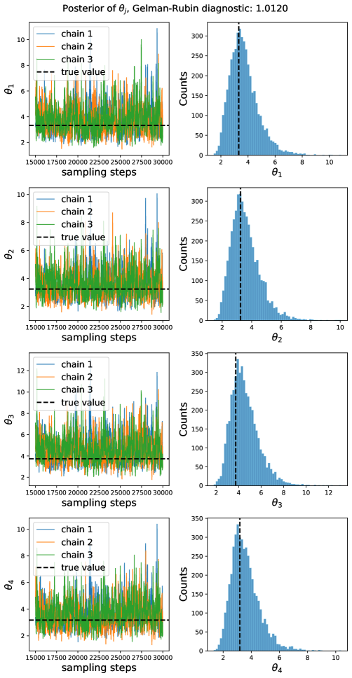
Figure 4: Posterior samples of $\theta_{j}$ for the data generated with $\alpha=0.2$.

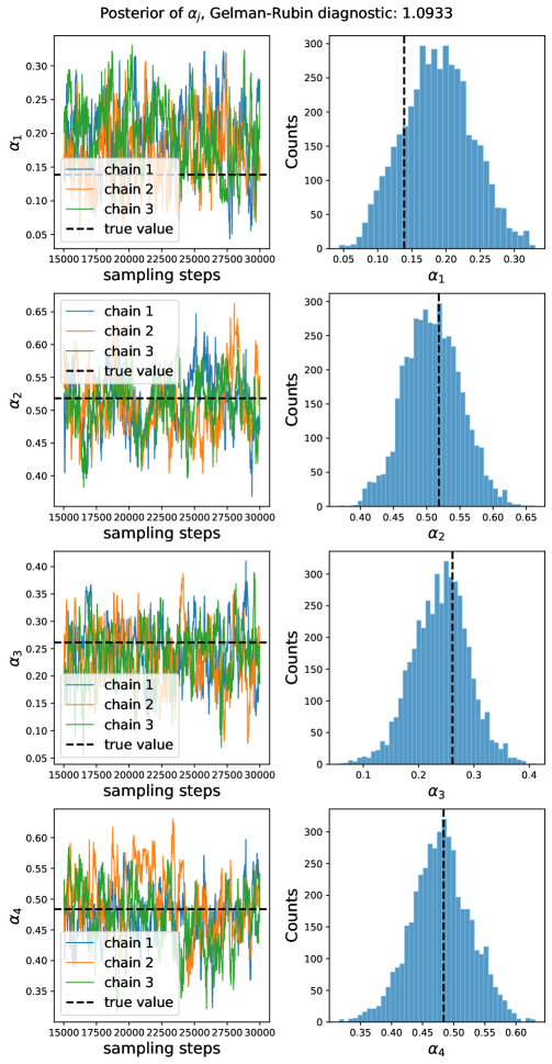
Figure 5: Posterior samples of $\alpha_{j}$ for the data generated with $\alpha=0.2$.

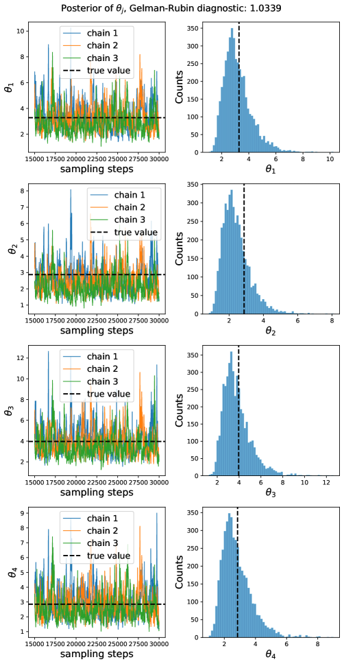
Figure 6: Posterior samples of $\theta_{j}$ for the data generated with $\alpha=0.6$.

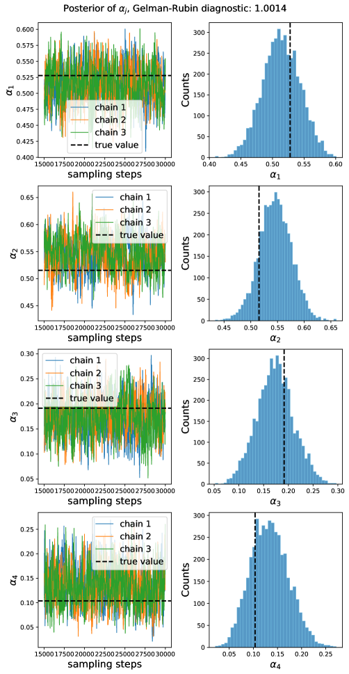
Figure 7: Posterior samples of $\alpha_{j}$ for the data generated with $\alpha=0.6$.

E.4 Predictions

According to Thereom 3, the predictive distribution is given as,

$$Z_{j}^{(M_{j}+1)}|((Z_{j}^{(i)},i\in[M_{j}]),j\in[J])$$

$$=\underbrace{\sum_{k=1}^{\xi(\phi_{j})}\bigg{[}\sum_{l=1}^{\tilde{X}_{j,k}}\tilde{A}^{(1)}_{j,k,l}\bigg{]}\delta_{Y_{j,k}}}_{\Circled{1}}+\underbrace{\sum_{k=1}^{r}\bigg{[}\sum_{l=1}^{\tilde{N}_{j,k}}\tilde{A}^{(2)}_{j,k,l}\bigg{]}\delta_{\tilde{Y}_{k}}}_{\Circled{2}}+\underbrace{\sum_{k=1}^{r}\bigg{[}\sum_{l=1}^{n_{j,k}}A_{j,k,l}\bigg{]}\delta_{\tilde{Y}_{k}}}_{\Circled{3}}$$

where each component is described in detail below.

1

Define

$$\gamma_{j}^{(M_{j}+1)} =\psi_{j}(M_{j}+1)-\psi_{j}(M_{j})=\theta_{j}\Psi_{\alpha_{j},\beta_{j}M_{j}+\zeta_{j}}(\beta_{j})$$ (E.26)

$$\tilde{\psi}_{0,J}(\gamma_{j}^{(M_{j}+1)}) =\tilde{\psi}_{0}(\gamma_{j}^{(M_{j}+1)}+\kappa)-\tilde{\psi}_{0}(\kappa)$$

$$=\theta_{0}\Psi_{\alpha,\kappa+\zeta}(\gamma_{j}^{(M_{j}+1)})$$ (E.27)

$$\tau_{0,J}(\lambda) =e^{-\lambda\kappa}\tau_{0}(\lambda)$$ (E.28)

$$\rho_{j}^{(M_{j})}(s) =e^{-\beta_{j}M_{j}}\rho_{j}(s).$$ (E.29)

Then we have

$$\xi(\phi_{j})\sim\mathrm{Poisson}(\gamma_{0}\tilde{\psi}_{0,J}(\gamma_{j}^{(M_{j}+1)})$$ (E.30)

$$(\tilde{X}_{j,k},k\in[r_{*}])|\xi(\phi_{j})=r_{*}\overset{\mathrm{i.i.d.}}{\sim}\mathrm{MtP}(\gamma_{j}^{(M_{j}+1)},\tau_{0,J}),$$ (E.31)

$$\mathbb{P}(\tilde{A}^{(1)}_{j,k,l}=m^{(1)}_{j,k,l},l\in[n_{j,k}^{(1)}])|\tilde{X}_{j,k}=n_{j,k}^{(1)})=\prod_{l=1}^{n_{j,k}^{(1)}}\mathsf{S}(m_{j,k,l}^{(1)}|\rho_{j}^{(M_{j})})$$ (E.32)

That is,

$$\mathbb{P}(\tilde{X}_{j,k}=n_{j,k}^{(1)}) =\int_{0}^{\infty}\frac{\lambda^{-\alpha-1}e^{-(\kappa+\zeta)\lambda}(1-e^{-\gamma_{j}^{(M_{j}+1)}\lambda})}{\Gamma(1-\alpha)\Psi_{\alpha,\kappa+\zeta}(\gamma_{j}^{(M_{j}+1)})}\frac{\mathds{1}_{\{n_{j,k}^{(1)}>0\}}(\gamma_{j}^{(M_{j}+1)}\lambda)^{n_{j,k}^{(1)}}e^{-\gamma_{j}^{(M_{j}+1)}\lambda}}{n_{j,k}^{(1)}!(1-e^{-\gamma_{j}^{(M_{j}+1)}\lambda})}d\lambda$$

$$=\frac{\mathds{1}_{\{n_{j,k}^{(1)}>0\}}(\gamma_{j}^{(M_{j}+1)})^{n_{j,k}^{(1)}}}{\Psi_{\alpha,\kappa+\zeta}(\gamma_{j}^{(M_{j}+1)})n_{j,k}^{(1)}!(\gamma_{j}^{(M_{j}+1)}+\kappa+\zeta)^{n_{j,k}^{(1)}-\alpha_{j}}}\frac{\Gamma(n_{j,k}^{(1)}-\alpha_{j})}{\Gamma(1-\alpha)},$$ (E.33)

so $\tilde{X}_{j,k}$ can be simulated as,

$$\mathbb{P}_{H_{0}}(d\lambda)=\frac{\lambda^{-\alpha-1}e^{-(\kappa+\zeta)\lambda}(1-e^{-\gamma_{j}^{(M_{j}+1)}\lambda})d\lambda}{\Gamma(1-\alpha)\Psi_{\alpha,\kappa+\zeta}(\gamma_{j}^{(M_{j}+1)})},$$ (E.34)

$$\mathbb{P}(\tilde{X}_{j,k}=n_{j,k}^{(1)}|H_{0}=\lambda)=\mathrm{tPoisson}(n_{j,k}^{(1)}|\gamma_{j}^{(M_{j}+1)}\lambda).$$ (E.35)

For $\tilde{A}^{(1)}_{j,k,l}$, we see that

$$\mathbb{P}(\tilde{A}^{(1)}_{j,k,l}=m_{j,k,l}^{(1)})$$

$$=\frac{\mathds{1}_{\{m_{j,k,l}^{(1)}>0\}}\int_{0}^{\infty}G_{A_{j}}(m_{j,k,l}^{(1)}|s)\rho_{j}^{(M_{j})}ds}{\gamma_{j}^{(M_{j}+1)}}$$

$$=\mathds{1}_{\{m_{j,k,l}^{(1)}>0\}}\int_{0}^{\infty}\frac{(\beta_{j}s)^{m_{j,k,l}^{(1)}}e^{-\beta_{j}s}}{m_{j,k,l}^{(1)}!}\frac{\theta_{j}s^{-\alpha_{j}-1}e^{-(\beta_{j}M_{j}+\zeta_{j})s}}{\Gamma(1-\alpha_{j})}\frac{1}{\theta_{j}\Psi_{\alpha_{j},\beta_{j}M_{j}+\zeta_{j}(\beta_{j})}}ds$$

$$=\mathds{1}_{\{m_{j,k,l}^{(1)}>0\}}\int_{0}^{\infty}\frac{(\beta_{j}s)^{m_{j,k,l}^{(1)}}e^{-\beta_{j}s}}{m_{j,k,l}^{(1)}!(1-e^{-\beta_{j}s})}\frac{s^{-\alpha_{j}-1}(1-e^{-\beta_{j}s})e^{-(\beta_{j}M_{j}+\zeta_{j})s}}{\Gamma(1-\alpha_{j})\Psi_{\alpha_{j},\beta_{j}M_{j}+\zeta_{j}}(\beta_{j})}ds$$

$$=\frac{\mathds{1}_{\{m_{j,k,l}^{(1)}>0\}}}{\Psi_{\alpha_{j},\beta_{j}M_{j}+\zeta_{j}}(\beta_{j})m_{j,k,l}^{(1)}!}\frac{\beta_{j}^{m_{j,k,l}^{(1)}}}{(\beta_{j}+\beta_{j}M_{j}+\zeta_{j})^{m_{j,k,l}^{(1)}-\alpha_{j}}}\frac{\Gamma(m_{j,k,l}^{(1)}-\alpha_{j})}{\Gamma(1-\alpha)}.$$ (E.36)

So each $\tilde{A}^{(1)}_{j,k,l}$ can be simulated as follows:

$$\mathbb{P}_{H_{j}^{(1)}}(ds)=\frac{s^{-\alpha_{j}-1}(1-e^{-\beta_{j}s})e^{-(\beta_{j}M_{j}+\zeta_{j})s}}{\Gamma(1-\alpha_{j})\Psi_{\alpha_{j},\beta_{j}M_{j}+\zeta_{j}}(\beta_{j})}ds$$ (E.37)

$$\mathbb{P}(\tilde{A}^{(1)}_{j,k,l}=m^{(1)}_{j,k,l}|H_{j}^{(1)}=s)=\mathrm{tPoisson}(m_{j,k,l}^{(1)}|\beta_{j}s).$$ (E.38)

2

For $\tilde{N}_{j,k}$, we have

$$\mathbb{P}_{\tilde{L}_{k}}(d\lambda) =\mathrm{Gamma}(n_{k}-\alpha,\kappa+\zeta),\quad\tilde{N}_{j,k}|\tilde{L}_{k}=\lambda\sim\mathrm{Poisson}(\gamma_{j}^{(M_{j}+1)}\lambda)$$ (E.39)

$$\mathbb{P}(\tilde{N}_{j,k}=n^{(2)}_{j,k}) =\frac{\Gamma(n_{j,k}^{(2)}+n_{k}-\alpha)}{(n_{j,k}^{(2)})!\Gamma(n_{k}-\alpha)}q_{j}^{n_{j,k}^{(2)}}(1-q_{j})^{n_{k}-\alpha}=\mathrm{NB}(n_{j,k}^{(2)}|n_{k}-\alpha,q_{j}),$$ (E.40)

where

$$q_{j}:=\frac{\gamma_{j}^{(M_{j}+1)}}{\gamma_{j}^{(M_{j}+1)}+\kappa+\zeta}.$$ (E.41)

$\tilde{A}_{j,k,l}^{(2)}$ has the same distribution as $\tilde{A}_{j,k,l}^{(1)}$.

$$\mathbb{P}(\tilde{A}^{(2)}_{j,k,l}=m_{j,k,l}^{(2)})=\frac{\mathds{1}_{\{m_{j,k,l}^{(2)}>0\}}}{\Psi_{\alpha_{j},\beta_{j}M_{j}+\zeta_{j}}(\beta_{j})m_{j,k,l}^{(2)}!}\frac{\beta_{j}^{m_{j,k,l}^{(2)}}}{(\beta_{j}+\beta_{j}M_{j}+\zeta_{j})^{m_{j,k,l}^{(2)}-\alpha_{j}}}\frac{\Gamma(m_{j,k,l}^{(2)}-\alpha_{j})}{\Gamma(1-\alpha)}.$$ (E.42)

3

For $A_{j,k,l}$, we have

$$\mathbb{P}_{S_{j,k,l}}(ds)=\mathrm{Gamma}(ds|m_{j,k,l}-\alpha_{j},\beta_{j}M_{j}+\zeta_{j}),$$ (E.43)

$$\mathbb{P}(A_{j,k,l}=m_{j,k,l}^{(3)}|S_{j,k,l}=s)=\mathrm{Poisson}(m_{j,k,l}^{(3)}|\beta_{j}s)$$ (E.44)

$$\mathbb{P}(A_{j,k,l}=m_{j,k,l}^{(3)})=\mathrm{NB}\bigg{(}m_{j,k,l}^{(3)}\big{|}m_{j,k,l}-\alpha_{j},\frac{\beta_{j}}{\beta_{j}+\beta_{j}M_{j}+\zeta_{j}}\bigg{)}.$$ (E.45)

E.5 Prediction with aggregated counts

Similar to the marginal likelihood, for a prediction, we don’t explicitly observe the separated counts $(\tilde{A}_{j,k,l}^{(1)}),(\tilde{A}_{j,k,l}^{(2)})$ and $(A_{j,k,l})$; we instead observe the aggregated counts for the new features (1) $\tilde{A}^{(1)}_{j,k}:=\sum_{l=1}^{\tilde{X}_{j,k}}\tilde{A}_{j,k}$, and the aggregated counts for the existing features (2 and 3) $\tilde{A}^{(2)}_{j,k}+A_{j,k}$ where $\tilde{A}^{(2)}_{j,k}:=\sum_{l=1}^{\tilde{N}_{j,k}}\tilde{A}^{(2)}_{j,k,l}$ and $A_{j,k}:=\sum_{l=1}^{n_{j,k}}A_{j,k,l}$. As before, we can compute the distribution for $\tilde{A}^{(1)}_{j,k}$ as

$$\mathbb{P}(\tilde{A}^{(1)}_{j,k}=m^{(1)}_{j,k}|\tilde{X}_{j,k}=n^{(1)}_{j,k})=\frac{\tilde{p}_{j}^{m^{(1)}_{j,k}}}{(1-(1-\tilde{p}_{j})^{\alpha_{j}})^{n^{(1)}_{j,k}}}\frac{n_{j,k}^{(1)}!\alpha_{j}^{n_{j,k}^{(1)}}S_{\alpha_{j}}(m_{j,k}^{(1)},n_{j,k}^{(1)})}{m_{j,k}^{(1)}!},$$ (E.46)

where

$$\tilde{p}_{j}=\frac{\beta_{j}}{\beta_{j}+\beta_{j}M_{j}+\zeta_{j}}.$$ (E.47)

Similarly,

$$\mathbb{P}(\tilde{A}^{(2)}_{j,k}=m^{(2)}_{j,k}|\tilde{N}_{j,k}=n^{(2)}_{j,k})=\frac{\tilde{p}_{j}^{m^{(2)}_{j,k}}}{(1-(1-\tilde{p}_{j})^{\alpha_{j}})^{n^{(2)}_{j,k}}}\frac{n_{j,k}^{(2)}!\alpha_{j}^{n_{j,k}^{(2)}}S_{\alpha_{j}}(m_{j,k}^{(2)},n_{j,k}^{(2)})}{m_{j,k}^{(2)}!},$$ (E.48)

For $A_{j,k}$,

$$\mathbb{P}(A_{j,k}=m_{j,k}^{(3)}|X_{j,k}=n_{j,k}) =\mathrm{NB}\bigg{(}m_{j,k}^{(3)}\big{|}m_{j,k}-n_{j,k}\alpha_{j},\frac{\beta_{j}}{\beta_{j}+\beta_{j}M_{j}+\zeta_{j}}\bigg{)}$$

$$=\frac{\Gamma(m_{j,k}^{(3)}+m_{j,k}-n_{j,k}\alpha_{j})}{m_{j,k}^{(3)}!\Gamma(m_{j,k}-n_{j,k}\alpha_{j})}\frac{\beta_{j}^{m_{j,k}^{(3)}}(\beta_{j}M_{j}+\zeta_{j})^{m_{j,k}-n_{j,k}\alpha_{j}}}{(\beta_{j}+\beta_{j}M_{j}+\zeta_{j})^{m_{j,k}^{(3)}+m_{j,k}-n_{j,k}\alpha_{j}}}.$$ (E.49)

Combining all these, the predictive likelihood with the aggregated counts is computed as

$$\mathbb{P}\Big{(}\xi(\phi_{j})=r_{*},(Y_{j,k}\in dy_{j,k}),(\tilde{X}_{j,k}=n_{j,k}^{(1)}),(\tilde{A}^{(1)}_{j,k}=m_{j,k}^{(1)}),(\tilde{N}_{j,k}=n_{j,k}^{(2)}),(\tilde{A}^{(2)}_{j,k}=m_{j,k}^{(2)}),((A_{j,k}=m_{j,k}^{(3)})\Big{)}$$

$$=\frac{\theta_{0}^{r_{*}}e^{-\gamma_{0}\theta_{0}\Psi_{\alpha,\kappa+\zeta}(\gamma_{j}^{(M_{j}+1)})}}{r_{*}!(\gamma_{j}^{(M_{j}+1)+\kappa+\zeta})^{n_{j}^{(1)}-r_{*}\alpha}}\prod_{k=1}^{r_{*}}\mathds{1}_{\{n_{j,k}^{(1)}>0\}}\frac{\Gamma(n_{j,k}^{(1)}-\alpha)}{\Gamma(1-\alpha)}G_{0}(dy_{j,k})$$

$$\times\prod_{k=1}^{r_{*}}\frac{\mathds{1}_{\{m_{j,k}^{(1)}\geq n_{j,k}^{(1)}\}}\theta_{j}^{n_{j,k}^{(1)}}\beta_{j}^{m_{j,k}^{(1)}}}{(\beta_{j}+\beta_{j}M_{j}+\zeta_{j})^{m_{j,k}^{(1)}-n_{j,k}^{(1)}\alpha_{j}}}\frac{S_{\alpha_{j}}(m_{j,k}^{(1)},n_{j,k}^{(1)})}{m_{j,k}^{(1)}!}$$

$$\times\frac{(\kappa+\zeta)^{n-r\alpha}}{(\gamma^{(M_{j}+1)}_{j}+\kappa+\zeta)^{n_{j}^{(2)}+n-r\alpha}}\prod_{k=1}^{r}\bigg{[}\frac{\Gamma(n_{j,k}^{(2)}+n_{k}-\alpha)}{\Gamma(n_{k}-\alpha)}\frac{\mathds{1}_{\{m_{j,k}^{(2)}\geq n_{j,k}^{(2)}\}}\theta_{j}^{n_{j,k}^{(2)}}\beta_{j}^{m_{j,k}^{(2)}}}{(\beta_{j}+\beta_{j}M_{j}+\zeta_{j})^{m_{j,k}^{(2)}-n_{j,k}^{(2)}\alpha_{j}}}\frac{S_{\alpha_{j}}(m_{j,k}^{(2)},n_{j,k}^{(2)})}{m_{j,k}^{(2)}!}\bigg{]}^{\mathds{1}_{\{n_{j,k}^{(2)}>0\}}}$$

$$\times\prod_{k=1}^{r}\frac{\Gamma(m_{j,k}^{(3)}+m_{j,k}-n_{j,k}\alpha_{j})}{m_{j,k}^{(3)}!\Gamma(m_{j,k}-n_{j,k}\alpha_{j})}\frac{\beta_{j}^{m_{j,k}^{(3)}}(\beta_{j}M_{j}+\zeta_{j})^{m_{j,k}-n_{j,k}\alpha_{j}}}{(\beta_{j}+\beta_{j}M_{j}+\zeta_{j})^{m_{j,k}^{(3)}+m_{j,k}-n_{j,k}\alpha_{j}}},$$ (E.50)

where $n^{(1)}_{j}:=\sum_{k=1}^{r_{*}}n_{j,k}^{(1)}$ and $n^{(2)}_{j}:=\sum_{k=1}^{r}n_{j,k}^{(2)}$. Given a new document $Z_{*}$, we can use the above predictive likelihood to compute the probability of $Z_{*}$ generated from the group $j$. However, as described above, since we only observe $\tilde{A}_{j,k}^{(1)}$ and $\tilde{A}_{j,k}^{(2)}+A_{j,k}$ values without $(\tilde{X}_{j,k}),(\tilde{N}_{j,k}),(\tilde{A}_{j,k}^{(2)})$, and $(A_{j,k})$, we cannot directly evaluate the predictive likelihood. Hence, we treat the missing variables as latents to be recovered via Gibbs sampling (assuming that we have resampled $X_{j,k}=n_{j,k}$ values during training).

Resampling $\tilde{X}_{j,k}$

The conditional distribution of $\tilde{X}_{j,k}$ given the others is,

$$\mathbb{P}(\tilde{X}_{j,k}=n_{j,k}^{(1)}|\tilde{A}^{(1)}_{j,k}=m_{j,k}^{(1)},\dots)$$

$$\propto\frac{\mathds{1}_{\{1\leq n_{j,k}^{(1)}\leq m_{j,k}^{(1)}\}}}{(\gamma_{j}^{(M_{j}+1)}+\kappa+\zeta)^{n_{j,k}^{(1)}}}\Gamma(n_{j,k}^{(1)}-\alpha)\theta_{j}^{n_{j,k}^{(1)}}(\beta_{j}+\beta_{j}M_{j}+\zeta_{j})^{\alpha_{j}n_{j,k}^{(1)}}S_{\alpha_{j}}(m_{j,k}^{(1)},n_{j,k}^{(1)}),$$ (E.51)

Resampling $\tilde{N}_{j,k}$, $\tilde{A}_{j,k}^{(2)}$ and $A_{j,k}$

Given $\tilde{A}^{(2)}_{j,k}+A_{j,k}=m_{j,k}^{(2,3)}$ and $X_{j,k}=n_{j,k}$, we have three possible cases:

1. $n_{j,k}=m_{j,k}^{(2,3)}=0$: we have $\tilde{N}_{j,k}=\tilde{A}_{j,k}^{(2)}=A_{j,k}=0$ with probability $1$.

2. $n_{j,k}=0$ and $m_{j,k}^{(2,3)}>0$: we have $\tilde{A}^{(2)}_{j,k}=m_{j,k}^{(2,3)}$ and $A_{j,k}=0$ with probability 1. Given $\tilde{A}^{(2)}_{j,k}=m_{j,k}^{(2,3)}$, the conditional distribution for $\tilde{N}_{j,k}$ is given as

   $$\mathbb{P}(\tilde{N}_{j,k}=n_{j,k}^{(2)}|\tilde{A}^{(2)}_{j,k}=m_{j,k}^{(2,3)},X_{j,k}=0,\dots)$$

   $$\propto\frac{\mathds{1}_{\{1\leq n_{j,k}^{(2)}\leq m_{j,k}^{(2,3)}\}}}{(\gamma_{j}^{(M_{j}+1)}+\kappa+\zeta)^{n_{j,k}^{(2)}}}\Gamma(n_{j,k}^{(2)}+n_{k}-\alpha)\theta_{j}^{n_{j,k}^{(2)}}(\beta_{j}+\beta_{j}M_{j}+\zeta_{j})^{\alpha_{j}n_{j,k}^{(2)}}S_{\alpha_{j}}(m_{j,k}^{(2)},n_{j,k}^{(2)}).$$ (E.52)

3. $n_{j,k}>0$ and $m_{j,k}^{(2,3)}>0$: the conditional distribution for $\tilde{N_{j,k}}$ is,

   $$\mathbb{P}(\tilde{N}_{j,k}=n_{j,k}^{(2)}|\tilde{A}^{(2)}_{j,k}+A_{j,k}=m_{j,k}^{(2,3)},X_{j,k}=n_{j,k},\dots)$$

   $$\propto\frac{\mathds{1}_{\{0\leq n_{j,k}^{(2)}\leq m_{j,k}^{(2,3)}\}}}{(\gamma_{j}^{(M_{j}+1)}+\kappa+\zeta)^{n_{j,k}^{(2)}}}\Gamma(n_{j,k}^{(2)}+n_{k}-\alpha)\theta_{j}^{n_{j,k}^{(2)}}(\beta_{j}+\beta_{j}M_{j}+\zeta_{j})^{\alpha_{j}n_{j,k}^{(2)}}$$

   $$\times\Big{(}S_{\alpha_{j}}(m_{j,k}^{(2)},n_{j,k}^{(2)})\Big{)}^{\mathds{1}_{\{n_{j,k}^{(2)}>0\}}}.$$ (E.53)

   Given $\tilde{N}_{j,k}=n_{j,k}^{(2)}$ drawn from the above conditional, if $n_{j,k}^{(2)}=0$, we have $\tilde{A}^{(2)}_{j,k}=0$ and $A_{j,k}=m_{j,k}^{(2,3)}$ with probability $1$. Otherwise, the conditional distribution for $\tilde{A}_{j,k}^{(2)}$ is,

   $$\mathbb{P}(\tilde{A}_{j,k}^{(2)}=m_{j,k}^{(2)}|\tilde{A}^{(2)}_{j,k}+A_{j,k}=m_{j,k}^{(2,3)},X_{j,k}=n_{j,k},\tilde{N}_{j,k}=n_{j,k}^{(2)},\dots)$$

   $$\propto\mathds{1}_{\{1\leq m_{j,k}^{(2)}\leq m_{j,k}^{(2,3)}\}}\frac{S_{\alpha_{j}}(m_{j,k}^{(2)},n_{j,k}^{(2)})}{m_{j,k}^{(2)}!}\frac{\Gamma(m_{j,k}^{(2,3)}-m_{j,k}^{(2)}+m_{j,k}-n_{j,k}\alpha_{j})}{(m_{j,k}^{(2,3)}-m_{j,k}^{(2)})!}$$ (E.54)

   After drawing $\tilde{A}_{j,k}^{(2)}=m_{j,k}^{(2)}$ with above, we have $A_{j,k}=m_{j,k}^{(2,3)}-m_{j,k}^{(2)}$ with probability $1$.

References

- [1] {barticle}[author] \bauthor\bsnmArgiento, \bfnmRaffaele\binitsR., \bauthor\bsnmCremaschi, \bfnmAndrea\binitsA. and \bauthor\bsnmVannucci, \bfnmMarina\binitsM. (\byear2020). \btitleHierarchical Normalized Completely Random Measures to Cluster Grouped Data. \bjournalJournal of the American Statistical Association \bvolume115 \bpages318-333. \endbibitem
- [2] {barticle}[author] \bauthor\bsnmAyed, \bfnmFadhel\binitsF. and \bauthor\bsnmCaron, \bfnmFrançois\binitsF. (\byear2021). \btitleNonnegative Bayesian nonparametric factor models with completely random measures. \bjournalStatistics and Computing \bvolume31 \bpages1–24. \endbibitem
- [3] {binproceedings}[author] \bauthor\bsnmBasbug, \bfnmMehmet\binitsM. and \bauthor\bsnmEngelhardt, \bfnmBarbara\binitsB. (\byear2016). \btitleHierarchical Compound Poisson Factorization. In \bbooktitleICML \bpages1795–1803. \bpublisherPMLR. \endbibitem
- [4] {barticle}[author] \bauthor\bsnmBenedetto, \bfnmGiuseppe Di\binitsG. D., \bauthor\bsnmCaron, \bfnmFrançois\binitsF. and \bauthor\bsnmTeh, \bfnmYee Whye\binitsY. W. (\byear2021). \btitleNonexchangeable random partition models for microclustering. \bjournalThe Annals of Statistics \bvolume49 \bpages1931 – 1957. \bdoi10.1214/20-AOS2003 \endbibitem
- [5] {barticle}[author] \bauthor\bsnmBlei, \bfnmDavid M\binitsD. M., \bauthor\bsnmNg, \bfnmAndrew Y\binitsA. Y. and \bauthor\bsnmJordan, \bfnmMichael I\binitsM. I. (\byear2003). \btitleLatent Dirichlet Allocation. \bjournalJournal of machine Learning research \bvolume3 \bpages993–1022. \endbibitem
- [6] {barticle}[author] \bauthor\bsnmBroderick, \bfnmTamara\binitsT., \bauthor\bsnmJordan, \bfnmMichael I\binitsM. I. and \bauthor\bsnmPitman, \bfnmJim\binitsJ. (\byear2013). \btitleCluster and feature modeling from combinatorial stochastic processes. \bjournalStatistical Science \bvolume28 \bpages289–312. \endbibitem
- [7] {barticle}[author] \bauthor\bsnmBroderick, \bfnmTamara\binitsT., \bauthor\bsnmMackey, \bfnmLester\binitsL., \bauthor\bsnmPaisley, \bfnmJohn\binitsJ. and \bauthor\bsnmJordan, \bfnmMichael I\binitsM. I. (\byear2014). \btitleCombinatorial clustering and the beta negative binomial process. \bjournalIEEE transactions on pattern analysis and machine intelligence \bvolume37 \bpages290–306. \endbibitem
- [8] {barticle}[author] \bauthor\bsnmBroderick, \bfnmTamara\binitsT., \bauthor\bsnmWilson, \bfnmAshia C\binitsA. C. and \bauthor\bsnmJordan, \bfnmMichael I\binitsM. I. (\byear2018). \btitlePosteriors, conjugacy, and exponential families for completely random measures. \bjournalBernoulli \bvolume24 \bpages3181–3221. \endbibitem
- [9] {barticle}[author] \bauthor\bsnmBrooks, \bfnmS. P.\binitsS. P. and \bauthor\bsnmGelman, \bfnmA.\binitsA. (\byear1997). \btitleGeneral methods for monitoring convergence of iterative simulations. \bjournalJournal of Computational and Graphical Statistics \bvolume7 \bpages434–455. \endbibitem
- [10] {barticle}[author] \bauthor\bsnmCamerlenghi, \bfnmFederico\binitsF., \bauthor\bsnmLijoi, \bfnmAntonio\binitsA., \bauthor\bsnmOrbanz, \bfnmPeter\binitsP. and \bauthor\bsnmPrünster, \bfnmIgor\binitsI. (\byear2019). \btitleDistribution theory for hierarchical processes. \bjournalThe Annals of Statistics \bvolume47 \bpages67–92. \endbibitem
- [11] {barticle}[author] \bauthor\bsnmCamerlenghi, \bfnmFederico\binitsF., \bauthor\bsnmLijoi, \bfnmAntonio\binitsA. and \bauthor\bsnmPrünster, \bfnmIgor\binitsI. (\byear2021). \btitleSurvival analysis via hierarchically dependent mixture hazards. \bjournalThe Annals of Statistics \bvolume49 \bpages863–884. \endbibitem
- [12] {barticle}[author] \bauthor\bsnmCampbell, \bfnmTrevor\binitsT., \bauthor\bsnmCai, \bfnmDiana\binitsD. and \bauthor\bsnmBroderick, \bfnmTamara\binitsT. (\byear2018). \btitleExchangeable trait allocations. \bjournalElectronic Journal of Statistics \bvolume12 \bpages2290–2322. \endbibitem
- [13] {barticle}[author] \bauthor\bsnmCaron, \bfnmFrançois\binitsF. (\byear2012). \btitleBayesian nonparametric models for bipartite graphs. \bjournalNeurIPS \bvolume25. \endbibitem
- [14] {barticle}[author] \bauthor\bsnmCaron, \bfnmFrançois\binitsF. and \bauthor\bsnmFox, \bfnmEmily B\binitsE. B. (\byear2017). \btitleSparse graphs using exchangeable random measures. \bjournalJournal of the Royal Statistical Society: Series B (Statistical Methodology) \bvolume79 \bpages1295–1366. \endbibitem
- [15] {binproceedings}[author] \bauthor\bsnmChen, \bfnmBo\binitsB., \bauthor\bsnmPolatkan, \bfnmGungor\binitsG., \bauthor\bsnmSapiro, \bfnmGuillermo\binitsG., \bauthor\bsnmCarin, \bfnmLawrence\binitsL. and \bauthor\bsnmDunson, \bfnmDavid B\binitsD. B. (\byear2011). \btitleThe hierarchical beta process for convolutional factor analysis and deep learning. In \bbooktitleICML \bpages361–368. \endbibitem
- [16] {barticle}[author] \bauthor\bsnmFerguson, \bfnmThomas S\binitsT. S. (\byear1973). \btitleA Bayesian Analysis of Some Non-parametric Problems. \bjournalThe Annals of Statistics \bvolume1 \bpages353–355. \endbibitem
- [17] {barticle}[author] \bauthor\bsnmGelman, \bfnmA.\binitsA. and \bauthor\bsnmRubin, \bfnmB.\binitsB. (\byear1992). \btitleInference from iterative simulation using multiple sequences. \bjournalStatistical Science \bvolume7 \bpages457–511. \endbibitem
- [18] {barticle}[author] \bauthor\bsnmGhahramani, \bfnmZoubin\binitsZ. and \bauthor\bsnmGriffiths, \bfnmThomas\binitsT. (\byear2005). \btitleInfinite latent feature models and the Indian Buffet Process. \bjournalNeurIPS \bvolume18. \endbibitem
- [19] {binproceedings}[author] \bauthor\bsnmGupta, \bfnmSunil Kumar\binitsS. K., \bauthor\bsnmPhung, \bfnmDinh\binitsD. and \bauthor\bsnmVenkatesh, \bfnmSvetha\binitsS. (\byear2012). \btitleA Bayesian nonparametric joint factor model for learning shared and individual subspaces from multiple data sources. \bpages200–211. \bpublisherSIAM. \endbibitem
- [20] {barticle}[author] \bauthor\bsnmHe, \bfnmShai\binitsS., \bauthor\bsnmSchein, \bfnmAaron\binitsA., \bauthor\bsnmSarsani, \bfnmVishal\binitsV. and \bauthor\bsnmFlaherty, \bfnmPatrick\binitsP. (\byear2021). \btitleA Bayesian nonparametric model for inferring subclonal populations from structured DNA sequencing data. \bjournalAOAS \bvolume15 \bpages925. \endbibitem
- [21] {barticle}[author] \bauthor\bsnmHeaukulani, \bfnmCreighton\binitsC. and \bauthor\bsnmRoy, \bfnmDaniel M\binitsD. M. (\byear2016). \btitleThe combinatorial structure of beta negative binomial processes. \bjournalBernoulli \bvolume22 \bpages2301–2324. \endbibitem
- [22] {barticle}[author] \bauthor\bsnmHjort, \bfnmNils Lid\binitsN. L. (\byear1990). \btitleNonparametric Bayes estimators based on beta processes in models for life history data. \bjournalthe Annals of Statistics \bpages1259–1294. \endbibitem
- [23] {barticle}[author] \bauthor\bsnmHo, \bfnmMan-Wai\binitsM.-W., \bauthor\bsnmJames, \bfnmLancelot F.\binitsL. F. and \bauthor\bsnmLau, \bfnmJohn W.\binitsJ. W. (\byear2021). \btitleGibbs partitions, Riemann–Liouville fractional operators, Mittag–Leffler functions, and fragmentations derived from stable subordinators. \bjournalJournal of Applied Probability \bvolume58 \bpages314–334. \bdoi10.1017/jpr.2020.93 \endbibitem
- [24] {barticle}[author] \bauthor\bsnmJames, \bfnmLancelot F\binitsL. F. (\byear2005). \btitleBayesian Poisson Process partition calculus with an application to Bayesian Lévy moving averages. \bjournalThe Annals of Statistics \bvolume33 \bpages1771–1799. \endbibitem
- [25] {barticle}[author] \bauthor\bsnmJames, \bfnmLancelot F\binitsL. F. (\byear2006). \btitlePoisson calculus for spatial neutral to the right processes. \bjournalThe annals of Statistics \bvolume34 \bpages416–440. \endbibitem
- [26] {barticle}[author] \bauthor\bsnmJames, \bfnmLancelot F.\binitsL. F. (\byear2010). \btitleDirichlet mean identities and laws of a class of subordinators. \bjournalBernoulli \bvolume16 \bpages361 – 388. \endbibitem
- [27] {barticle}[author] \bauthor\bsnmJames, \bfnmLancelot F\binitsL. F. (\byear2017). \btitleBayesian Poisson calculus for latent feature modeling via generalized Indian Buffet Process priors. \bjournalThe Annals of Statistics \bvolume45 \bpages2016–2045. \endbibitem
- [28] {barticle}[author] \bauthor\bsnmJames, \bfnmLancelot F\binitsL. F., \bauthor\bsnmLee, \bfnmJuho\binitsJ. and \bauthor\bsnmPandey, \bfnmAbhinav\binitsA. (\byear2021). \btitlePosterior distributions for Hierarchical Spike and Slab Indian Buffet processes. \bjournalarXiv preprint arXiv:2103.11407. \endbibitem
- [29] {barticle}[author] \bauthor\bsnmJames, \bfnmLancelot F\binitsL. F., \bauthor\bsnmLijoi, \bfnmAntonio\binitsA. and \bauthor\bsnmPrünster, \bfnmIgor\binitsI. (\byear2009). \btitlePosterior analysis for normalized random measures with independent increments. \bjournalScandinavian Journal of Statistics \bvolume36 \bpages76–97. \endbibitem
- [30] {barticle}[author] \bauthor\bsnmKarlis, \bfnmDimitris\binitsD. and \bauthor\bsnmXekalaki, \bfnmEvdokia\binitsE. (\byear2005). \btitleMixed poisson distributions. \bjournalInternational Statistical Review/Revue Internationale de Statistique \bpages35–58. \endbibitem
- [31] {binproceedings}[author] \bauthor\bsnmKessler, \bfnmSamuel\binitsS., \bauthor\bsnmNguyen, \bfnmVu\binitsV., \bauthor\bsnmZohren, \bfnmStefan\binitsS. and \bauthor\bsnmRoberts, \bfnmStephen J\binitsS. J. (\byear2021). \btitleHierarchical indian buffet neural networks for bayesian continual learning. In \bbooktitleUAI \bpages749–759. \bpublisherPMLR. \endbibitem
- [32] {barticle}[author] \bauthor\bsnmKingman, \bfnmJohn FC\binitsJ. F. (\byear1975). \btitleRandom discrete distributions. \bjournalJRSSB \bvolume37 \bpages1–15. \endbibitem
- [33] {barticle}[author] \bauthor\bsnmKnowles, \bfnmDavid\binitsD. and \bauthor\bsnmGhahramani, \bfnmZoubin\binitsZ. (\byear2011). \btitleNonparametric Bayesian sparse factor models with application to gene expression modeling. \bjournalAOAS \bvolume5 \bpages1534–1552. \endbibitem
- [34] {barticle}[author] \bauthor\bsnmLo, \bfnmAlbert Y\binitsA. Y. (\byear1982). \btitleBayesian nonparametric statistical inference for Poisson point processes. \bjournalZeitschrift für Wahrscheinlichkeitstheorie und verwandte Gebiete \bvolume59 \bpages55–66. \endbibitem
- [35] {binproceedings}[author] \bauthor\bsnmMasoero, \bfnmL\binitsL., \bauthor\bsnmCamerlenghi, \bfnmF\binitsF., \bauthor\bsnmFavaro, \bfnmS\binitsS. and \bauthor\bsnmBroderick, \bfnmT\binitsT. (\byear2018). \btitlePosterior representations of hierarchical completely random measures in trait allocation models. In \bbooktitleBNP-NeurIPS. \endbibitem
- [36] {barticle}[author] \bauthor\bsnmMasoero, \bfnmLorenzo\binitsL., \bauthor\bsnmCamerlenghi, \bfnmFederico\binitsF., \bauthor\bsnmFavaro, \bfnmStefano\binitsS. and \bauthor\bsnmBroderick, \bfnmTamara\binitsT. (\byear2022). \btitleMore for less: predicting and maximizing genomic variant discovery via Bayesian nonparametrics. \bjournalBiometrika \bvolume109 \bpages17–32. \endbibitem
- [37] {barticle}[author] \bauthor\bsnmPitman, \bfnmJim\binitsJ. (\byear1997). \btitlePartition structures derived from Brownian motion and stable subordinators. \bjournalBernoulli \bpages79–96. \endbibitem
- [38] {barticle}[author] \bauthor\bsnmPitman, \bfnmJim\binitsJ. (\byear2017). \btitleMixed Poisson and negative binomial models for clustering and species sampling. Manuscript in preparation. \bjournalManuscript in preparation. \endbibitem
- [39] {barticle}[author] \bauthor\bsnmQuenouille, \bfnmM. H.\binitsM. H. (\byear1949). \btitleA Relation between the Logarithmic, Poisson, and Negative Binomial Series. \bjournalBiometrics \bvolume5 \bpages162–164. \endbibitem
- [40] {barticle}[author] \bauthor\bsnmSchein, \bfnmAaron\binitsA. (\byear2019). \btitleAllocative poisson factorization for computational social science. \endbibitem
- [41] {barticle}[author] \bauthor\bsnmTeh, \bfnmYee\binitsY. and \bauthor\bsnmGorur, \bfnmDilan\binitsD. (\byear2009). \btitleIndian buffet processes with power-law behavior. \bjournalNeurIPS \bvolume22. \endbibitem
- [42] {binproceedings}[author] \bauthor\bsnmTeh, \bfnmYee Whye\binitsY. W. (\byear2006). \btitleA hierarchical Bayesian language model based on Pitman-Yor processes. \bpages985–992. \endbibitem
- [43] {barticle}[author] \bauthor\bsnmTeh, \bfnmYee Whye\binitsY. W., \bauthor\bsnmJordan, \bfnmMichael I\binitsM. I., \bauthor\bsnmBeal, \bfnmMatthew J\binitsM. J. and \bauthor\bsnmBlei, \bfnmDavid M\binitsD. M. (\byear2006). \btitleHierarchical Dirichlet Processes. \bjournalJournal of the American Statistical Association \bvolume101 \bpages1566-1581. \endbibitem
- [44] {binproceedings}[author] \bauthor\bsnmThibaux, \bfnmRomain\binitsR. and \bauthor\bsnmJordan, \bfnmMichael I\binitsM. I. (\byear2007). \btitleHierarchical beta processes and the Indian buffet process. \bpages564–571. \bpublisherPMLR. \endbibitem
- [45] {barticle}[author] \bauthor\bsnmTitsias, \bfnmMichalis\binitsM. (\byear2007). \btitleThe infinite gamma-Poisson feature model. \bjournalNeurIPS \bvolume20. \endbibitem
- [46] {barticle}[author] \bauthor\bsnmTodeschini, \bfnmAdrien\binitsA., \bauthor\bsnmMiscouridou, \bfnmXenia\binitsX. and \bauthor\bsnmCaron, \bfnmFrançois\binitsF. (\byear2020). \btitleExchangeable random measures for sparse and modular graphs with overlapping communities. \bjournalJRSSB \bvolume82 \bpages487–520. \endbibitem
- [47] {barticle}[author] \bauthor\bsnmWood, \bfnmFrank\binitsF., \bauthor\bsnmGasthaus, \bfnmJan\binitsJ., \bauthor\bsnmArchambeau, \bfnmCédric\binitsC., \bauthor\bsnmJames, \bfnmLancelot\binitsL. and \bauthor\bsnmTeh, \bfnmYee Whye\binitsY. W. (\byear2011). \btitleThe sequence memoizer. \bjournalCommunications of the ACM \bvolume54 \bpages91–98. \endbibitem
- [48] {barticle}[author] \bauthor\bsnmZhou, \bfnmMingyuan\binitsM. and \bauthor\bsnmCarin, \bfnmLawrence\binitsL. (\byear2013). \btitleNegative binomial process count and mixture modeling. \bjournalIEEE Transactions on Pattern Analysis and Machine Intelligence \bvolume37 \bpages307–320. \endbibitem
- [49] {barticle}[author] \bauthor\bsnmZhou, \bfnmMingyuan\binitsM., \bauthor\bsnmFavaro, \bfnmStefano\binitsS. and \bauthor\bsnmWalker, \bfnmStephen G\binitsS. G. (\byear2017). \btitleFrequency of frequencies distributions and size-dependent exchangeable random partitions. \bjournalJASA \bvolume112 \bpages1623–1635. \endbibitem
- [50] {barticle}[author] \bauthor\bsnmZhou, \bfnmMingyuan\binitsM., \bauthor\bsnmPadilla, \bfnmOscar Hernan Madrid\binitsO. H. M. and \bauthor\bsnmScott, \bfnmJames G\binitsJ. G. (\byear2016). \btitlePriors for random count matrices derived from a family of negative binomial processes. \bjournalJASA \bvolume111 \bpages1144–1156. \endbibitem