Local conditions for global convergence
of gradient flows and proximal point sequences
in metric spaces

Abstract.

This paper deals with local criteria for the convergence to a global minimiser for gradient flow trajectories and their discretisations. To obtain quantitative estimates on the speed of convergence, we consider variations on the classical Kurdyka–Łojasiewicz inequality for a large class of parameter functions. Our assumptions are given in terms of the initial data, without any reference to an equilibrium point. The main results are convergence statements for gradient flow curves and proximal point sequences to a global minimiser, together with sharp quantitative estimates on the speed of convergence. These convergence results apply in the general setting of lower semicontinuous functionals on complete metric spaces, generalising recent results for smooth functionals on ${\mathbb{R}}^{n}$. While the non-smooth setting covers very general spaces, it is also useful for (non)-smooth functionals on ${\mathbb{R}}^{n}$.

1. Introduction

For given $x_{0}\in{\mathbb{R}}^{n}$ and $f\in\mathrm{C}^{2}({\mathbb{R}}^{n})$ we consider the gradient flow equation

$$\tfrac{\mathrm{d}}{\mathrm{d}t}y_{t}=-\nabla f(y_{t})\,\mathrm{,}\;\,\qquad y_{0}=x_{0}\,\mathrm{.}$$ (1.1)

It is of great interest in many applications to find conditions which guarantee convergence of gradient-flow trajectories $\left(y_{t}\right)_{t\geq 0}$ to a global minimiser of $f$ as $t\to\infty$, and to quantify the speed of convergence. This also applies to the associated discrete-time schemes, such as gradient descent (or forward Euler), the discrete-time scheme with step-size $\tau>0$ given by

$$y_{k+1}=y_{k}-\tau\nabla f(y_{k})\,\mathrm{,}\;\,\qquad y_{0}=x_{0}\,\mathrm{,}\;\,$$ (1.2)

and the backward Euler scheme

$$y_{k+1}=y_{k}-\tau\nabla f(y_{k+1})\,\mathrm{,}\;\,\qquad y_{0}=x_{0}\,\mathrm{.}$$ (1.3)

The Polyak–Łojasiewicz condition

A very simple celebrated criterion for convergence to a global minimum is the Polyak–Łojasiewicz condition [30], which requires neither the uniqueness of a minimiser nor the convexity of the function $f$. The condition holds if, for some $\beta>0$,

$$|\nabla f(x)|^{2}\geq\beta(f(x)-f^{\star})\,\mathrm{,}\;\,\qquad x\in{\mathbb{R}}^{n}\,\mathrm{,}\;\,$$ (PŁ)

where $f^{\star}$ is the global minimum of $f$, which is assumed to be attained. Since $\tfrac{\mathrm{d}}{\mathrm{d}t}f(y_{t})=-|\nabla f(y_{t})|^{2}$ along any solution $y_{t}$ to the gradient-flow equation $\tfrac{\mathrm{d}}{\mathrm{d}t}y_{t}=-\nabla f(y_{t})$, an application of Gronwall’s inequality yields the exponential bound

$$f(y_{t})-f^{\star}\leq e^{-\beta t}\big{(}f(y_{0})-f^{\star}\big{)}\,\mathrm{,}\;\,\qquad t\geq 0\,\mathrm{.}$$

Moreover, a short argument shows that $y_{t}$ converges to a global minimiser $x^{\star}$, with the bound

$$|y_{t}-x^{\star}|^{2}\leq\frac{4}{\beta}\big{(}f(y_{t})-f^{\star}\big{)}\,\mathrm{,}\;\,\qquad t\geq 0\,\mathrm{.}$$

These inequalities together yield exponentially fast convergence to $x^{\star}$. Analogous results hold for the associated gradient-descent scheme (1.2) and for certain proximal-gradient methods [19]. Interestingly, in spite of its simplicity, it has been argued in [19] that the PŁ condition «is actually weaker than the main conditions that have been explored to show linear convergence rates without strong convexity over the last 25 years.»

The Kurdyka–Łojasiewicz condition

An important generalization of the PŁ condition is the Kurdyka–Łojasiewicz inequality (KŁ), that was introduced by Łojasiewicz [23, 24] and later generalized by Kurdyka [21].

Definition 1.1.

Let $\theta\in C([0,\infty))\cap C^{1}((0,\infty))$ satisfy $\theta(0)=0$ and $\theta^{\prime}(u)>0$ for $u>0$. We say that the KŁ inequality is satisfied in a neighbourhood $U$ of an equilibrium point $x^{\star}\in{\mathbb{R}}^{n}$ if

$$\theta^{\prime}(f(x)-f(x^{\star}))\cdot|\nabla f(x)|\geq 1\qquad\text{ for all }\;x\in U\cap\left\{f>f(x^{\star})\right\}.$$ (1.4)

In applications, $\theta$ is often of the form $\theta(u)\coloneqq\frac{c}{\gamma}u^{\gamma}$ with $\gamma\in(0,1]$ and $c>0$. In this case, (1.4) reads as

$$c\,|\nabla f(x)|\geq\big{(}{f(x)-f(x^{\star})}\big{)}^{1-\gamma}\,\mathrm{,}\;\,\qquad x\in U\cap\left\{f>f(x^{\star})\right\}\,\mathrm{.}$$

In particular, if $\gamma=\frac{1}{2}$ and $c=1/\sqrt{\beta}$ one recovers the PŁ inequality.

The KŁ condition is a powerful tool to obtain convergence properties for gradient-flow solutions and discrete schemes. An important feature of the KŁ condition is that the inequality is only required to hold locally, on a suitable neighbourhood $U$ of an equilibrium point.

To obtain convergence results for gradient-flow trajectories to an equilibrium point, the KŁ condition is often combined with additional information, typically an upper bound on the length of the trajectory, to ensure that the solution is eventually contained in $U$; cf. [32, 15] for results of this type for gradient flows and [3, 4, 5, 8] for discrete schemes.

Let us also remark that the KŁ condition does not in general yield convergence to a global minimiser of $f$, but merely to a stationary point. To deduce convergence to a global minimiser, it is often required to know a priori that the starting point is close enough to this minimiser (whose existence is often part of the assumption); cf. [4, Thm. 10] and [5, Thm. 2.12] for such results for discrete schemes.

A PŁ condition around the starting point

A remarkable variant of the PŁ condition was discussed by Oymak and Soltanolkotabi [29] and by Chatterjee [12] for non-negative functions $f\in\mathrm{C}^{2}({\mathbb{R}}^{n})$. For fixed $x_{0}\in{\mathbb{R}}^{n}$, these authors consider the local quantity

$$\alpha=\alpha(x_{0},r)\operatorname{\coloneqq}\inf_{\begin{subarray}{c}x\in B_{r}(x_{0})\\ f(x)\neq 0\end{subarray}}\frac{|\nabla f(x)|^{2}}{f(x)}\,\mathrm{,}\;\,$$

where $B_{r}(x_{0})$ denotes the open ball of radius $r>0$ around $x_{0}$. The criterion in [12] requires that

$$\alpha(x_{0},r)>\frac{4f(x_{0})}{r^{2}}$$ (1.5)

for some $x_{0}\in{\mathbb{R}}^{n}$ and some $r>0$. In other words, the inequality $|\nabla f(x)|^{2}\geq\beta f(x)$ is imposed to hold for all $x\in B_{r}(x_{0})$, with a sufficiently large constant $\beta$, namely, $\beta>4f(x_{0})/r^{2}$.

Under (1.5), it is shown in [12] that the unique gradient flow curve $(y_{t})_{t\geq 0}$ starting at $y_{0}=x_{0}$ stays within $B_{r}(x_{0})$ for all times $t\geq 0$, converges to a global minimiser $x^{\star}\in\overline{B_{r}(x_{0})}$, and satisfies the exponential bounds

$$f(y_{t})\leq e^{-\alpha t}f(x_{0})\quad{\rm and}\quad|y_{t}-x^{\star}|^{2}\leq r^{2}e^{-\alpha t}$$ (1.6)

for $t\geq 0$, where we write $\alpha=\alpha(x_{0},r)$ for brevity.

Like the KŁ condition, (1.5) is a local version of the PŁ condition. However, while the KŁ condition involves information of $f$ in a neighbourhood of an equilibrium point (whose location is often unknown in applications), (1.5) is formulated in terms of the starting point $x_{0}$ of the gradient-flow trajectory. The existence of a global minimiser and the boundedness of the gradient-flow trajectory are not assumed; these statements are part of the conclusion. The specific constant $\frac{4f(x_{0})}{r^{2}}$ in (1.5) is important, as it ensures that the gradient-flow curve does not leave the ball $B_{r}(x_{0})$, so that local information suffices to draw conclusions on the long-term behaviour.

Chatterjee also proves analogous bounds for the gradient descent (1.2) starting at $y_{0}=x_{0}$, namely

$$f(y_{k})\leq(1-\delta)^{k}f(x_{0})\quad{\rm and}\quad|y_{k}-x^{\star}|\leq r^{2}(1-\delta)^{k}$$

for all $k\in{\mathbb{N}}$ and any $\delta<\alpha\tau$, provided that the step-size $\tau>0$ is sufficiently small, depending also on the size of the derivatives of $f$ in $B_{r}(x_{0})$. Similar results for gradient descent were obtained previously in [29]. Applications of (1.5) to neural networks can be found in [29, 11, 12, 10, 6].

1.1. Main results

In this work we generalise some of the results of [12] in the following ways. First, we replace $\mathrm{C}^{2}$ functions on ${\mathbb{R}}^{n}$ with lower semicontinuous functionals on complete metric spaces. Secondly, we replace the local PŁ-like condition with a KŁ-like assumption with a more general parameter function $\theta$. Thirdly, we prove convergence results for the proximal point method, which corresponds to the backward Euler scheme in smooth settings.

Let $(X,\mathsf{d})$ be a complete metric space. In this generality, the ode (1.1) does not have a direct interpretation, as the velocity of a curve and the gradient of a function are not defined. However (1.1) admits an equivalent variational characterisation, as a curve of maximal slope, and this notion naturally extends to metric spaces. We refer to Section 2 for the definition of the metric slope $\left\lvert\mathrm{D}^{-}{f}\right\rvert\!(x)$ and other concepts from analysis in metric spaces relevant to our work. Gradient flows in metric spaces are ubiquitous in applications; notable examples are dissipative pdes in the Wasserstein space [18, 2] and related gradient flows on spaces of (probability) measures; see, e.g., [13, 25, 27, 20]. A systematic treatment can be found in the monograph [1]. The metric point of view can also be useful to deal with non-differentiable functionals on ${\mathbb{R}}^{n}$; see §4 for some toy examples.

We first define the functions appearing in the assumption and the main results.

Definition 1.2 (Parameter function).

We say that $\theta\in C^{1}((0,\infty))\cap C([0,\infty))$ is a parameter function if $\theta^{\prime}(u)>0$ for $u>0$, and $\theta(0)=0$. Furthermore, we consider the auxiliary functions $\eta:[0,\infty)\to[-\infty,\infty)$ and $\Gamma:[0,\theta(\infty))\to[-\infty,\infty)$ defined by

$$\eta(u):=\int_{1}^{u}\big{(}\theta^{\prime}(s)\big{)}^{2}\mathop{}\!\mathrm{d}s\quad{\rm and}\quad\Gamma(u):=(\eta\circ\theta^{-1})(u).$$

The next definition contains a generalisation of (1.5) to the metric setting for a general class of parameter functions; see Remark 4.1 below for a precise comparison.

Definition 1.3 (Conditions $(A)$ and $(A^{\prime})$).

For $x_{0}\in\mathrm{dom}(f)$ and $r>0$, we say that condition $(A)$ is satisfied with parameter function $\theta$ (as in Definition 1.2) if

$$(\theta\circ f)(x_{0})\leq r\quad\text{and}\quad(\theta^{\prime}\circ f)(x)\cdot\left\lvert\mathrm{D}^{-}{f}\right\rvert\!(x)\geq 1\,\mathrm{,}\;\,\quad x\in B_{r}(x_{0})\cap\left\{0<f\leq f(x_{0})\right\}\,\mathrm{.}$$ (1.7)

Similarly, we say that condition $(A^{\prime})$ is satisfied if the first inequality in (1.7) is replaced by the strict inequality $(\theta\circ f)(x_{0})<r$.

Under Condition $(A)$, our first main result asserts that gradient-flow trajectories stay within in a bounded set and converge to a global minimum, with quantitative bounds on the rate of convergence.

Theorem 1.4 (Convergence of gradient flows).

Let $f:X\to[0,\infty]$ be proper and lower semicontinuous, and suppose that $x_{0}\in\mathrm{dom}(f)$ and $r>0$ satisfy Condition $(A)$ for some parameter function $\theta$. For some $T\in(0,\infty]$, let $\left(y_{t}\right)_{t\in[0,T)}$ be a curve of maximal slope for $f$ starting at $x_{0}$. Then:

1. (confinement) $y_{t}\in\overline{B_{r}(x_{0})}$ for all $0\leq t<T$. Moreover, $y_{t}\in B_{r}(x_{0})$ for all $0\leq t<T$ with $f(y_{t})>0$.

2. (convergence) $y_{T}\operatorname{\coloneqq}\lim_{t\to T}y_{t}$ exists and belongs to $\overline{B_{r}(x_{0})}$. Moreover,

   $$(\theta\circ f)(y_{s})-(\theta\circ f)(y_{t})\geq\mathsf{d}(y_{t},y_{s})$$ (1.8)

   for all $0\leq s\leq t\leq T$. In particular, $y_{T}\in B_{r}(x_{0})$ if $f(y_{T})>0$.

3. (convergence rates) Set $t_{*}\coloneqq\inf\left\{t\in[0,T):f(y_{t})=0\right\}\wedge T$. The following bounds hold for $0\leq t\leq t_{*}$:

   $$\Gamma\big{(}\mathsf{d}(y_{t},y_{T})\big{)} \leq\Gamma(r)-t,$$ (1.9)

   $$(\eta\circ f)(y_{t}) \leq(\eta\circ f)(x_{0})-t.$$ (1.10)

   Moreover, if $T=\infty$ then $f(y_{\infty})=0$.

In the special case of Remark 4.1, the previous theorem yields the following generalisation of [12, Thm. 2.1] to the setting of metric spaces; see also Cor. 3.8 below for a version with more general parameter functions. For $x_{0}\in\mathrm{dom}(f)$ and $r>0$ we define

$$\alpha=\alpha(x_{0},r)\operatorname{\coloneqq}\inf_{\begin{subarray}{c}x\in B_{r}(x_{0})\\ 0<f(x)\leq f(x_{0})\end{subarray}}\frac{\left\lvert\mathrm{D}^{-}{f}\right\rvert\!(x)^{2}}{f(x)}\,.$$

Corollary 1.5.

Let $f:X\to[0,\infty]$ be proper and lower semicontinuous, and suppose that $\alpha(x_{0},r)\geq 4f(x_{0})/r^{2}$ for some  $x_{0}\in\mathrm{dom}(f)$ and $r>0$. For some $T\in(0,\infty]$, let $\left(y_{t}\right)_{t\in[0,T)}$ be a curve of maximal slope for $f$ starting at $x_{0}$. Then $y_{T}\coloneqq\lim_{t\to T}y_{t}$ exists, $y_{t}$ belongs to $\overline{B_{r}(x_{0})}$ for all $t\in[0,T]$, and

$$\mathsf{d}(y_{t},y_{T})\leq r\,e^{-\alpha t/2}\qquad\text{and}\qquad f(y_{t})\leq e^{-\alpha t}f(x_{0})$$

for all $t\in[0,T]$, where, conventionally, $e^{-\infty}\operatorname{\coloneqq}0$.

Various works deal with convergence of gradient-flow trajectories under a KŁ condition in the setting of metric spaces [7, 15]; see also [8, 3, 4] for related work on proximal point sequences. Applications have been found to convergence of mean-field birth-death processes [22] and to swarm gradient dynamics [9].

The main estimates in our paper are obtained by adapting known arguments from, e.g., [7, 15]. However, as in [29, 12], our point of view differs from these works, as we work under a local condition in terms of the starting point without referring to an equilibrium point in the assumption.

Discrete schemes

In the general setting of metric spaces, we are not aware of any way to formulate a forward Euler scheme (1.2). However, the backward Euler scheme admits an equivalent metric formulation as a minimising movement scheme (or proximal point method). This scheme was originally introduced by Martinet [26] and Rockafellar [31] as a natural regularisation method in optimisation problems:

$$y_{k+1}\in\operatorname*{arg\,min}_{x\in X}\bigg{\{}f(x)+\frac{1}{2\tau}\mathsf{d}(y_{k},x)^{2}\bigg{\}}\,\mathrm{,}\;\,\qquad y_{0}=x_{0}\,\mathrm{.}$$

Any (finite or infinite) sequence $\left(y_{k}\right)_{k}$ arising in this way is called a proximal point sequence (or $\tau$-minimising movement sequence).

Our second main result is an analogue of Theorem 1.4 for the proximal point method, under the slightly stronger assumption $(A^{\prime})$.

Theorem 1.6.

Let $f:X\to[0,\infty]$ be proper and lower semicontinuous, and suppose that $x_{0}\in\mathrm{dom}(f)$ and $r>0$ satisfy Condition $(A^{\prime})$ for some parameter function $\theta$. Suppose further that there exists $\bar{\tau}>0$ such that, for all $x\in B_{r}(x_{0})\cap\left\{f\leq f(x_{0})\right\}$ and $\tau\in(0,\bar{\tau})$, the functional

$$X\ni y\longmapsto f(x)+\frac{1}{2\tau}\mathsf{d}(x,y)^{2}$$

has at least one global minimiser. Then there exists an infinite proximal point sequence starting from $x_{0}$, for any step-size $\tau<\bar{\tau}$. Moreover, for any such sequence $(y_{k})_{k=0}^{\infty}$, the following statements hold:

1. (confinement) $y_{k}\in B_{r}(x_{0})$ for all $k\geq 0$;

2. (convergence) $y_{\infty}\operatorname{\coloneqq}\lim_{k\to\infty}y_{k}$ exists and belongs to $B_{r}(x_{0})$. Moreover, $f(y_{\infty})=0$;

3. (distance bound) For all $0\leq i\leq j<\infty$ we have

   $$\mathsf{d}(y_{i},y_{j})\leq(\theta\circ f)(y_{i})-(\theta\circ f)(y_{j})\quad\text{and}\quad\mathsf{d}(y_{i},y_{\infty})\leq(\theta\circ f)(y_{i})\,\mathrm{.}$$ (1.11)

In the particular case where $\theta$ takes the form $\theta(u)\coloneqq 2c\sqrt{u}$, we obtain the following result. In this case we also obtain an estimate for the speed of convergence of $f(y_{k})$ to $0$. Other special cases of Theorem 1.6 are presented in Corollary 6.7 below.

Corollary 1.7 (see Cor. 6.7).

Let $f:X\to[0,\infty]$ be proper and lower semicontinuous, and suppose that and suppose that $\alpha(x_{0},r)>4f(x_{0})/r^{2}$ for some  $x_{0}\in\mathrm{dom}(f)$ and $r>0$. Suppose further that there exists $\bar{\tau}>0$ such that, for all $x\in B_{r}(x_{0})\cap\left\{f\leq f(x_{0})\right\}$ and $\tau\in(0,\bar{\tau})$, the functional

$$X\ni y\longmapsto f(x)+\frac{1}{2\tau}\mathsf{d}(x,y)^{2}$$

has at least one global minimiser. Then there exists an infinite proximal point sequence starting from $x_{0}$, for any step-size $\tau<\bar{\tau}$. Moreover, for any such sequence, the following statements hold:

1. (confinement) $y_{k}\in B_{r}(x_{0})$ for all $k\geq 0$;

2. (convergence) $y_{\infty}\operatorname{\coloneqq}\lim_{k\to\infty}y_{k}$ exists and belongs to $B_{r}(x_{0})$. Moreover, $f(y_{\infty})=0$;

3. (convergence rates) The following bounds hold for all $k\geq 0$:

   $$f(y_{k}) \leq\big{(}1+{\alpha\tau}\big{)}^{-k}f(x_{0})\quad{\rm and}\quad\mathsf{d}(y_{k},y_{\infty})\leq\big{(}1+{\alpha\tau}\big{)}^{-k/2}\,r\,\mathrm{.}$$

Plan of the work

Preliminaries on gradient flows in metric spaces are collected in §2. Our main results in the continuum case are proved in §3 and extended to piecewise gradient-flow curves in §5. In §4 we discuss Condition $(A)$ and its variants together with some examples. Our main results in the discrete case are proved in §6. Auxiliary results are presented in the appendices.

Acknowledgement

The authors gratefully acknowledges support by the European Research Council (ERC) under the European Union’s Horizon 2020 research and innovation programme (grant agreement No. 716117). LDS gratefully acknowledges funding of his current position by the Austrian Science Fund (FWF), ESPRIT Fellowship Project 208. JM also acknowledges support by the Austrian Science Fund (FWF), Project SFB F65.

2. Gradient flows in metric spaces

In this section we collect some known facts about gradient flows in metric spaces. We assume throughout that  $(X,\mathsf{d})$ is a complete metric space and $J\subset{\mathbb{R}}$ is a (not necessarily open, nor closed) interval.

Let $1\leq p<\infty$. A measurable function $m:J\to{\mathbb{R}}$ belongs to  $L^{p}_{\mathrm{loc}}(J)$ if ${\bf 1}_{K}m\in L^{p}(J)$ for every compact set $K\subset J$. A curve $\left(y_{t}\right)_{t\in J}$ is said to be locally $p$-absolutely continuous on $J$ —in short: it belongs to $\mathrm{AC}^{p}_{\mathrm{loc}}(J;X)$— if there exists $m\in L^{p}_{\mathrm{loc}}(J)$ so that

$$\mathsf{d}(y_{t},y_{s})\leq\int_{s}^{t}m(r)\mathop{}\!\mathrm{d}r$$ (2.1)

for all $s,t\in J$ with $s<t$. Similarly, we write  $\left(y_{t}\right)_{t\in J}\in\mathrm{AC}^{p}(J;X)$ if $m\in L^{p}(J)$.

Whenever $\left(y_{t}\right)_{t\in J}$ is in $\mathrm{AC}^{1}_{\mathrm{loc}}(J;X)$, the metric speed

$$\left\lvert\dot{y}_{t}\right\rvert\operatorname{\coloneqq}\lim_{s\to t}\frac{\mathsf{d}(y_{s},y_{t})}{\left\lvert s-t\right\rvert}$$ (2.2)

exists for a.e. $t\in J$. Furthermore, the metric speed coincides a.e. with the smallest function  $m$ satisfying (2.1); see, e.g., [1, Thm. 1.1.2].

Remark 2.1.

Every curve in $\mathrm{AC}^{1}_{\mathrm{loc}}(J;X)$ is continuous on $J$. Note however that if $\left(y_{t}\right)_{t\in J}\in\mathrm{AC}^{1}_{\mathrm{loc}}(J;X)$ with  $J=(a,b]$ for some $a<b$, then the existence of $\lim_{t\downarrow a}y_{t}$ does not imply that $\left(y_{t}\right)_{t\in J}\in\mathrm{AC}^{1}(J;X)$.

The domain of a function $f\colon X\to(-\infty,\infty]$ is the set

$$\mathrm{dom}(f)\operatorname{\coloneqq}\left\{x\in X:f(x)<\infty\right\}\,\mathrm{.}$$

In order to rule out trivial statements, we always assume that $f$ is proper, i.e., $\mathrm{dom}(f)\neq\operatorname{\varnothing}$. The (descending) slope of $f$ at $x\in X$ is the quantity

$$\left\lvert\mathrm{D}^{-}{f}\right\rvert\!(x)\operatorname{\coloneqq}\limsup_{y\to x}\frac{\big{[}f(y)-f(x)\big{]}_{-}}{\mathsf{d}(y,x)}\,\mathrm{,}\;\,$$

where $a_{-}\operatorname{\coloneqq}\max\left\{-a,0\right\}$ denotes the negative part of $a\in{\mathbb{R}}$. Conventionally, $\left\lvert\mathrm{D}^{-}{f}\right\rvert\!(x)\operatorname{\coloneqq}0$ when $x\in\mathrm{dom}(f)$ is isolated, and $\left\lvert\mathrm{D}^{-}{f}\right\rvert\!(x)=+\infty$ if $x\notin\mathrm{dom}(f)$.

2.1. Gradient flows in metric spaces: curves of maximal slope

The next definition provides a natural notion of gradient flow in a metric space; cf. [1] for an extensive treatment. The motivation for this definition comes from the following simple argument in Euclidean space. Let $f\colon{\mathbb{R}}^{n}\to{\mathbb{R}}$ be a smooth function. For any smooth curve $(u_{t})_{t\in[0,T)}$ in ${\mathbb{R}}^{n}$ and $t\in(0,T)$, we have

$$-\tfrac{\mathrm{d}}{\mathrm{d}t}f(u_{t})=-\nabla f(u_{t})\cdot\dot{u}_{t}\leq\tfrac{1}{2}|\nabla f(u_{t})|^{2}+\tfrac{1}{2}|\dot{u}_{t}|^{2}\,\mathrm{.}$$

Since equality holds if and only if $\dot{u}_{t}=-\nabla f(u_{t})$, the reverse inequality $-\tfrac{\mathrm{d}}{\mathrm{d}t}f(u_{t})\geq\frac{1}{2}|\nabla f(u_{t})|^{2}+\frac{1}{2}|\dot{u}_{t}|^{2}$ is an equivalent formulation of the gradient-flow equation, which admits a natural generalisation to metric spaces.

Definition 2.2 (curve of maximal slope, gradient flow, cf. [28, Dfn. 4.1]).

Let $J\subset{\mathbb{R}}$ be an interval and let $f:X\to(-\infty,\infty]$ be proper. We say that $\left(y_{t}\right)_{t\in J}$ is a curve of maximal slope for $f$ if

1. $\left(y_{t}\right)_{t\in J}\in\mathrm{AC}^{1}_{\mathrm{loc}}(J;X)$;

2. $\left(f(y_{t})\right)_{t\in J}\in\mathrm{AC}^{1}_{\mathrm{loc}}(J;{\mathbb{R}})$;

3. the following Energy Dissipation Inequality holds:

   $$-\tfrac{\mathrm{d}}{\mathrm{d}t}f(y_{t})\geq\tfrac{1}{2}\left\lvert\dot{y}_{t}\right\rvert^{2}+\tfrac{1}{2}\left\lvert\mathrm{D}^{-}{f}\right\rvert\!(y_{t})^{2}\quad{\textrm{\,for ${\mathop{}\!\mathrm{d}t}$-a.e.~{}}}t\in J\,\mathrm{.}$$ (edi)

If additionally  $y_{\inf J}\operatorname{\coloneqq}\lim_{t\downarrow\inf J}y_{t}$ exists, we say that $\left(y_{t}\right)_{t\in J}$ is a curve of maximal slope for $f$ starting at $y_{\inf J}$.

Remark 2.3.

From (edi) and the absolute continuity of $f$ we conclude that $t\mapsto f(y_{t})$ is non-increasing along curves of maximal slope $\left(y_{t}\right)_{t\in[0,T)}$.

There are several slightly different notions of curve of maximal slope in the literature, and the distinction matters for our purposes. In particular, it is important here to include the absolute continuity of the function along gradient-flow trajectories in our definition, as this allows one to deduce the following well-known fact, asserting the equality of the speed of the gradient flow and the slope of the driving functional.

Lemma 2.4.

Let $f:X\to(-\infty,\infty]$ be proper and let $\left(y_{t}\right)_{t\in J}$ be a curve of maximal slope. For a.e. $t\in J$ we have

$$-\tfrac{\mathrm{d}}{\mathrm{d}t}f(y_{t})=\left\lvert\dot{y}_{t}\right\rvert^{2}=\left\lvert\mathrm{D}^{-}{f}\right\rvert\!(y_{t})^{2}.$$ (2.3)

In particular, equality holds for a.e. $t\in{J}$ in (edi).

Proof.

Let $t\in J$ be such that the metric speed $\left\lvert\dot{y}_{t}\right\rvert$ and the derivative $\tfrac{\mathrm{d}}{\mathrm{d}t}f(y_{t})$ exist. By local absolute continuity of $(y_{t})_{t}$ and $(f(y_{t}))_{t}$, this property holds almost everywhere. Using the definitions we obtain

$$-\tfrac{\mathrm{d}}{\mathrm{d}t}f(y_{t})=\limsup_{s\downarrow t}\frac{f(y_{t})-f(y_{s})}{|t-s|}\leq\limsup_{s\downarrow t}\frac{f(y_{t})-f(y_{s})}{\mathsf{d}(y_{t},y_{s})}\cdot\limsup_{s\downarrow t}\frac{\mathsf{d}(y_{t},y_{s})}{|t-s|}\leq\left\lvert\mathrm{D}^{-}{f}\right\rvert\!(y_{t})\cdot\left\lvert\dot{y}_{t}\right\rvert.$$

Combining this inequality with (edi), we find that

$$\tfrac{1}{2}\left\lvert\dot{y}_{t}\right\rvert^{2}+\tfrac{1}{2}\left\lvert\mathrm{D}^{-}{f}\right\rvert\!(y_{t})^{2}\leq-\tfrac{\mathrm{d}}{\mathrm{d}t}f(y_{t})\leq\left\lvert\mathrm{D}^{-}{f}\right\rvert\!(y_{t})\cdot\left\lvert\dot{y}_{t}\right\rvert,$$

which, again by Young’s inequality, implies the desired identities. ∎

In light of Lemma 2.4, every curve of maximal slope satisifies the Energy Dissipation Equality for a.e.  $t\in J$:

$$-\tfrac{\mathrm{d}}{\mathrm{d}t}f(y_{t})=\tfrac{1}{2}\left\lvert\dot{y}_{t}\right\rvert^{2}+\tfrac{1}{2}\left\lvert\mathrm{D}^{-}{f}\right\rvert\!(y_{t})^{2}.$$ (ede)

Remark 2.5.

Let $J=[a,b)$ with $-\infty<a<b\leq\infty$ and suppose that $y_{a}\in\mathrm{dom}(f)$. If $f$ is bounded from below by some constant $M\in{\mathbb{R}}$, then $t\mapsto\left\lvert\dot{y}_{t}\right\rvert$ belongs to $L^{2}(a,b)$ for every curve of maximal slope $(y_{t})_{t\in J}$. Indeed, for $t\in(a,b)$, integration of (edi) yields

$$\frac{1}{2}\int_{a}^{t}\left\lvert\dot{y}_{r}\right\rvert^{2}\mathop{}\!\mathrm{d}r+\frac{1}{2}\int_{a}^{t}\left\lvert\mathrm{D}^{-}{f}\right\rvert\!{(y_{r})}^{2}\mathop{}\!\mathrm{d}r\leq f(y_{a})-f(y_{t})\leq f(y_{a})-M.$$ (2.4)

The conclusion follows by passing to the limit $t\uparrow b$.

Remark 2.6 (Comparison with [15, Dfn.s 2.12, 2.13]).

Our Definition 2.2 is more restrictive than [15, Dfn.s 2.12, 2.13] as we additionally require the condition in b. This condition guarantees that $\left\lvert\mathrm{D}^{-}{f}\right\rvert\!$ is a strong upper gradient of $f$ along $\left(y_{t}\right)_{t\in J}$; see e.g. [2, Rmk. 2.8]. Furthermore, by b we may integrate (edi) to conclude that $t\mapsto f(y_{t})$ is non-increasing, which is rather an assumption in [15, Dfn. 2.12]. Everywhere below, following [15], we could drop the assumption of b and replace $\left\lvert\mathrm{D}^{-}{f}\right\rvert\!$ by any given strong upper gradient $g$. For the sake of simplicity however, we confine our exposition to the case $g\operatorname{\coloneqq}\left\lvert\mathrm{D}^{-}{f}\right\rvert\!$ for which the assumptions in [15] are verified in light of b as discussed above.

3. Convergence of gradient flows

This section is devoted to the proof of Theorem 1.4, which deals with the converence of gradient flows under Assumption $(A)$.

Definition 3.1 (Equilibrium point).

We say that  $x^{\star}\in X$ is an equilibrium point for $f$ if $x^{\star}\in\mathrm{dom}(\left\lvert\mathrm{D}^{-}{f}\right\rvert\!)$ and  $\left\lvert\mathrm{D}^{-}{f}\right\rvert\!(x^{\star})=0$.

We refer to cf. [15, Dfn. 2.35] for a more general definition for strong upper gradients.

Clearly, every local minimiser $x^{\star}\in\mathrm{dom}(f)$ is an equilibrium point for $f$.

It will be useful to first investigate gradient flow curves starting from an equilibrium point.

Lemma 3.2 (Trivial flows).

Let $f\colon X\to(-\infty,\infty]$ be proper and $T\in(0,\infty]$.

1. If $x^{\star}\in\mathrm{dom}(f)$ is an equilibrium point for $f$, then the constant curve $\left(y_{t}\right)_{t\in[0,T)}$ defined by $y_{t}\equiv x^{\star}$ is a curve of maximal slope for $f$ starting at $x^{\star}$.

2. If $x^{\star}\in\mathrm{dom}(f)$ is a local minimiser for $f$, then the constant curve $\left(y_{t}\right)_{t\in[0,T)}$ defined by $y_{t}\equiv x^{\star}$ is the only curve of maximal slope for $f$ starting at $x^{\star}$.

Proof.

$(i)$:  This follows immediately from the definitions.

$(ii)$:  Let $x^{\star}\in\mathrm{dom}(f)$ be a local minimiser and let $U$ be a neighbourhood of $x^{\star}$ such that  $f\geq f(x^{\star})$ on $U$. Furthermore, let $\left(y_{t}\right)_{t\in[0,T)}$ be a curve of maximal slope for $f$ starting at $x^{\star}$, and set

$$t_{0}\operatorname{\coloneqq}\inf\left\{t>0:y_{t}\notin U\right\}\wedge T\,\mathrm{.}$$

Note that $t_{0}>0$, since $t\mapsto y_{t}$ is continuous. Since $y_{t}\in U$ for $t\in[0,t_{0})$, we have $f(y_{t})\geq f(x^{\star})$ for $t\in[0,t_{0})$. As $t\mapsto f(y_{t})$ is non-increasing by  (edi), we thus infer that $f(y_{t})=f(x^{\star})$ for $t\in[0,t_{0})$. Therefore, $t\mapsto\tfrac{\mathrm{d}}{\mathrm{d}t}f(y_{t})$ is identically $0$, hence $\left\lvert\dot{y}_{t}\right\rvert=0$ for $t\in[0,t_{0})$ again by (edi). Applying (2.1) to the metric speed, we infer that  $\mathsf{d}(y_{t},y_{0})\leq\int_{0}^{t}\left\lvert\dot{y}_{r}\right\rvert\mathop{}\!\mathrm{d}r=0$, hence $y_{t}=y_{0}\operatorname{\coloneqq}x^{\star}$ for all $t\in[0,t_{0})$. By continuity of $t\mapsto y_{t}$ we conclude that $t_{0}=T$, which proves the assertion. ∎

For convenience of the reader we recall the following definition from the introduction.

Definition 3.3 (Auxiliary function).

Given a parameter function $\theta:[0,\infty)\to[0,\infty)$ we consider the auxiliary function

$$\eta:[0,\infty)\to[-\infty,\infty),\qquad \eta(u) :=\int_{1}^{u}\big{(}\theta^{\prime}(s)\big{)}^{2}\mathop{}\!\mathrm{d}s\qquad\text{for $u\in[0,\infty)$},$$

$$\Gamma:[0,\theta(\infty))\to[-\infty,\infty),\qquad \Gamma(u) :=(\eta\circ\theta^{-1})(u).$$

Here we use the convention that $\theta(\infty):=\lim_{u\to\infty}\theta(u)$. Note that $\theta$ is indeed invertible and nonnegative, so that $\Gamma$ is well-defined. The following lemma collects some elementary properties of $\theta$. We leave the proof to the reader.

Lemma 3.4 (Properties of the auxiliary function).

The function $\eta$ is strictly increasing, $\eta(1)=0$, and $\eta(0)$ is possibly $-\infty$. Moreover, $\eta$ is continuously differentiable on $(0,\infty)$ and $\eta^{\prime}(u)=(\theta^{\prime}(u))^{2}$ for all $u>0$.

Remark 3.5.

In the special case where $\theta(u)=\frac{c}{\gamma}u^{\gamma}$ we have the explicit formulas

$$\eta(u)=\frac{c^{2}}{2\gamma-1}(u^{2\gamma-1}-1)\quad\text{if $\gamma>0,\ \gamma\neq\frac{1}{2}$},\qquad\text{and}\qquad\eta(u)=c^{2}\log u\quad\text{if $\gamma=\frac{1}{2}$}\,\mathrm{.}$$

The following lemma contains the crucial quantitative bounds on the distance and the driving functional that can be derived from Condition $(A)$, for suitable gradient-flow trajectories that stay within the ball $B_{r}(x_{0})$.

Lemma 3.6 (Distance bound and energy bound).

Let $f\colon X\to[0,\infty]$ be lower semicontinuous, and suppose that $x_{0}\in\mathrm{dom}(f)$ and $r>0$ satisfy Condition $(A)$ for some parameter function $\theta$. Let $\left(y_{t}\right)_{t\in[0,T)}$, with $T\in(0,\infty]$, be a curve of maximal slope starting at $x_{0}$. Let $0\leq s\leq t<T$ and assume that $y_{u}\in B_{r}(x_{0})$ and $f(y_{u})>0$ for all $u\in[s,t]$. Then:

$$(\theta\circ f)(y_{s})-(\theta\circ f)(y_{t}) \geq\mathsf{d}(y_{t},y_{s}),$$ (3.1)

$$(\eta\circ f)(y_{s})-(\eta\circ f)(y_{t}) \geq t-s.$$ (3.2)

Proof.

As $\theta$ and $\eta$ are continuously differentiable on $(0,\infty)$, and  $t\mapsto f(y_{t})$ is locally absolute continuous, we conclude that also  $\mathcal{H}\colon t\mapsto(\theta\circ f)(y_{t})$ and $t\mapsto(\eta\circ f)(y_{t})$ are locally absolutely continuous on $(0,T)$. For almost every $u\in[s,t]$, we obtain by absolute continuity of $\mathcal{H}$, by (2.3), and by $(A)$,

$$-\mathcal{H}^{\prime}(u)=-(\theta^{\prime}\circ f)(y_{u})\cdot\tfrac{\mathrm{d}}{\mathrm{d}u}f(y_{u})=(\theta^{\prime}\circ f)(y_{u})\cdot\left\lvert\mathrm{D}^{-}{f}\right\rvert\!(y_{u})\left\lvert\dot{y}_{u}\right\rvert\geq\left\lvert\dot{y}_{u}\right\rvert.$$ (3.3)

Since $t\mapsto y_{t}$ is locally absolute continuous, we obtain

$$\mathsf{d}(y_{t},y_{s})\leq\int_{s}^{t}\left\lvert\dot{y}_{u}\right\rvert\mathop{}\!\mathrm{d}u\leq\int_{s}^{t}-\mathcal{H}^{\prime}(u)\mathop{}\!\mathrm{d}u=\mathcal{H}(s)-\mathcal{H}(t),$$ (3.4)

which proves (3.1).

Moreover, using again that $f(y_{u})>0$ for all $u\in[s,t]$, we obtain for a.e. $u\in(s,t)$, by Lemma 3.4, by Lemma 2.4, and by $(A)$,

$$-\tfrac{\mathrm{d}}{\mathrm{d}u}(\eta\circ f)(y_{u})=-(\eta^{\prime}\circ f)(y_{u})\cdot\tfrac{\mathrm{d}}{\mathrm{d}u}f(y_{u})=\Big{(}(\theta^{\prime}\circ f)(y_{u})\cdot\left\lvert\mathrm{D}^{-}{f}\right\rvert\!(y_{u})\Big{)}^{2}\geq 1.$$

Integration of this inequality yields (3.2). ∎

Example 3.7.

An explicit computation shows that in the special case where $\theta(u)=\frac{c}{\gamma}u^{\gamma}$, the energy estimate (3.2) becomes

$$f(y_{t}) \leq\begin{cases}\displaystyle\bigg{(}f(y_{s})^{2\gamma-1}-\frac{2\gamma-1}{c^{2}}(t-s)\bigg{)}^{1/(2\gamma-1)}&\text{ if }\gamma>0\,\mathrm{,}\;\,\gamma\neq\frac{1}{2}\,\mathrm{,}\\ e^{-(t-s)/c^{2}}f(y_{s})&\text{ if }\gamma=\frac{1}{2}\,\mathrm{.}\end{cases}$$ (3.5)

We are now ready to prove our first main result.

Proof of Theorem 1.4.

We assume that $f(x_{0})>0$, as the result would otherwise follow immediately from Lemma 3.2.

i  We define

$$t_{0}\operatorname{\coloneqq}\inf\big{\{}t\in[0,T):y_{t}\in\partial B_{r}(x_{0})\big{\}}\wedge T$$

and note that $t_{0}>0$, since $(y_{t})_{t\in[0,T)}$ is continuous. If $t_{0}=T$ the conclusion follows, hence it suffices to treat the case where $t_{0}<T$.

If $f(y_{t_{0}})=0$, the conclusion follows from Lemma 3.2 and the definition of $t_{0}$. It thus remains to treat the case where $t_{0}<T$ and $f(y_{t_{0}})>0$. We will show that these conditions yield a contradiction, which completes the proof.

Indeed, (3.1) and Assumption $(A)$ yield, for $0<t<t_{0}$,

$$\mathsf{d}(y_{t},x_{0}) \leq(\theta\circ f)(x_{0})-(\theta\circ f)(y_{t})\leq r-(\theta\circ f)(y_{t_{0}})\,\mathrm{.}$$

Since $(\theta\circ f)(y_{t_{0}})>0$ and $t\mapsto y_{t}$ is continuous, it follows by passing to the limit $t\uparrow t_{0}$ that $\mathsf{d}(y_{t_{0}},x_{0})<r$. This is the desired contradiction, since $\mathsf{d}(y_{t_{0}},x_{0})=r$ by construction.

ii  Since $t\mapsto f(y_{t})$ is continuous, it follows that

$$t_{*}\operatorname{\coloneqq}\inf\left\{t\in[0,T):f(y_{t})=0\right\}\wedge T>0\,\mathrm{.}$$

We first claim that $y_{T}\operatorname{\coloneqq}\lim_{t\to T}y_{t}$ exists and belongs to $\overline{B_{r}(x_{0})}$.

If $t_{*}<T$, then $y_{t}=y_{t_{*}}$ for every $t\in[t_{*},T)$ by Lemma 3.2, and the claim follows.

If otherwise $t_{*}=T$, then (3.1) holds for all $0\leq s\leq t<T$. Write $\mathcal{H}(t)\operatorname{\coloneqq}(\theta\circ f)(y_{t})$. Then $\mathcal{H}\colon[0,T)\to[0,\infty)$ is continuous, non-increasing and bounded from below, so it admits a continuous non-increasing extension on $[0,T]$. Thus, the bound (for $0\leq s<t<T$)

$$\mathsf{d}(y_{s},y_{t})\leq\mathcal{H}(s)-\mathcal{H}(t)\leq\mathcal{H}(s)-\mathcal{H}(T)$$

combined with $\mathcal{H}(s)\downarrow\mathcal{H}(T)\geq 0$ as $s\to T$ implies the Cauchy property of $\left(y_{t}\right)_{t}$, hence the existence of the limit, which proves the claim.

By lower semicontinuity of $f$ and Lemma 3.2 and in view of i, we infer that (3.1) holds for all $0\leq s\leq t\leq T$ (even if $t_{*}<T$). Choosing $s=0$ and $t=T$, the last part of the statement follows using 1.7.

iii  Let $0\leq t<t_{*}$. In view of i, (1.10) follows from (3.2). Next, by (1.8) we have

$$\mathsf{d}(y_{t},y_{T})\leq\theta(f(y_{t}))-\theta(f(y_{T}))\leq\theta(f(y_{t})).$$

Using this bound and (1.10), we obtain

$$(\eta\circ\theta^{-1})(\mathsf{d}(y_{t},y_{T}))\leq(\eta\circ f)(y_{t})\leq(\eta\circ f)(x_{0})-t\leq(\eta\circ\theta^{-1})(r)-t,$$

which shows (1.9). By continuity of $(y_{t})_{t}$ and lower semicontinuity of $f$, (1.9) and (1.10) extend to $t=t_{*}$.

Finally, suppose that $T=\infty$. If $t_{*}<\infty$, then clearly $f(y_{\infty})=0$. If on the other hand $t_{*}=\infty$, it follows from (1.10) that $(\eta\circ f)(y_{t})\to-\infty$ as $t\to\infty$, hence $f(y_{t})\to 0$. By lower semicontinuity of $f$ the result follows. ∎

In the special case where the parameter function $\theta$ takes the form $\theta(u)=\frac{c}{\gamma}u^{\gamma}$, we obtain the following more explicit result. The notation $t^{*}$ was introduced in Theorem 1.4.

Corollary 3.8.

Let $f\colon X\to[0,\infty]$ be lower semicontinuous and suppose that $x_{0}\in\mathrm{dom}(f)$ and $r>0$ satisfy Condition $(A)$ with parameter function $\theta(u)=\tfrac{c}{\gamma}u^{\gamma}$ for some $c>0$ and $\gamma\in(0,1]$. Let $\left(y_{t}\right)_{t\in[0,T)}$ be a curve of maximal slope for $f$ starting at $x_{0}$, for some $T\in(0,\infty]$. Then $y_{T}\coloneqq\lim_{t\to T}y_{t}$ exists, $y_{t}$ belongs to $\overline{B_{r}(x_{0})}$ for all $t\in[0,T]$, and for all $0\leq t\leq t^{*}$ we have

$$\mathsf{d}(y_{t},y_{T}) \leq\frac{c}{\gamma}\bigg{(}\Big{(}\frac{\gamma r}{c}\Big{)}^{\frac{2\gamma-1}{\gamma}}-\frac{2\gamma-1}{c^{2}}t\bigg{)}^{\frac{\gamma}{2\gamma-1}}, f(y_{t}) \leq\bigg{(}f(x_{0})^{2\gamma-1}-\frac{2\gamma-1}{c^{2}}t\bigg{)}^{\frac{1}{2\gamma-1}}, \text{if }\gamma \neq\tfrac{1}{2}\,\mathrm{,}\;\,$$ (3.6)

$$\mathsf{d}(y_{t},y_{T}) \leq re^{-\frac{t}{2c^{2}}}, f(y_{t}) \leq f(x_{0})\,e^{-\frac{t}{c^{2}}}, \text{if }\gamma =\tfrac{1}{2}\,\mathrm{.}$$ (3.7)

Moreover, if $\frac{1}{2}<\gamma\leq 1$, we have $t_{*}\leq\frac{c^{2}}{2\gamma-1}f(x_{0})^{2\gamma-1}$.

Proof.

The estimates for $\mathsf{d}(y_{t},y_{T})$ and $f(y_{t})$ are obtained from (1.9) and (1.10) by rearranging terms. The final assertion follows from the second bound in (3.6). ∎

Remark 3.9 (The case $\theta(u)=\tfrac{c}{2}\sqrt{u}$).

Under the above assumptions, the distance estimate in Corollary 3.8 can be improved if $\gamma=\frac{1}{2}$, using the following the ideas of [12]. Let $0\leq s\leq t\leq T$ and assume that $y_{u}\in B_{r}(x_{0})$ and $f(y_{u})>0$ for all $u\in[s,t]$. Then:

$$\mathsf{d}(y_{t},y_{s})^{2} \leq 4c^{2}\Big{(}e^{-\frac{s}{2c^{2}}}-e^{-\frac{t}{2c^{2}}}\Big{)}\sqrt{f(x_{0})}\Big{(}\sqrt{f(y_{s})}-\sqrt{f(y_{t})}\Big{)}$$ (3.8)

$$\leq 4c^{2}e^{-\frac{s}{2c^{2}}}\Big{(}e^{-\frac{s}{2c^{2}}}-e^{-\frac{t}{2c^{2}}}\Big{)}f(x_{0})\,\mathrm{.}$$ (3.9)

Proof.

We can assume $t<T$ and then extend the result to $t=T$ by taking limits. Using the local 2-absolute continuity of $\left(y_{t}\right)_{t\in[0,T)}$, the Cauchy–Schwarz inequality, and the assumption that $f(y_{u})>0$ for all $u\in[s,t]$, we find

$$\mathsf{d}(y_{t},y_{s})\leq\int_{s}^{t}\left\lvert\dot{y}_{u}\right\rvert\mathop{}\!\mathrm{d}u\leq\left(\int_{s}^{t}\sqrt{f(y_{u})}\mathop{}\!\mathrm{d}u\right)^{1/2}\left(\int_{s}^{t}\frac{\left\lvert\dot{y}_{u}\right\rvert^{2}}{\sqrt{f(y_{u})}}\mathop{}\!\mathrm{d}u\right)^{1/2}\,\mathrm{.}$$ (3.10)

By local absolute continuity of $u\mapsto f(y_{u})$ we see that $u\mapsto\sqrt{f(y_{u})}$ too is locally absolutely continuous, and $\tfrac{\mathrm{d}}{\mathrm{d}u}\sqrt{f(y_{u})}(t)=\big{(}2\sqrt{f(y_{u})}\big{)}^{-1}\tfrac{\mathrm{d}}{\mathrm{d}u}f(y_{u})$ holds a.e. on $(0,T)$. Since $\tfrac{\mathrm{d}}{\mathrm{d}u}f(y_{u})=-\left\lvert\dot{y}_{u}\right\rvert^{2}$ by  (2.3), we obtain

$$\int_{s}^{t}\frac{\left\lvert\dot{y}_{u}\right\rvert^{2}}{\sqrt{f(y_{u})}}\mathop{}\!\mathrm{d}u=-\int_{s}^{t}\frac{\tfrac{\mathrm{d}}{\mathrm{d}u}f(y_{u})}{\sqrt{f(y_{u})}}\mathop{}\!\mathrm{d}u=-2\int_{s}^{t}\tfrac{\mathrm{d}}{\mathrm{d}u}\sqrt{f(y_{u})}\mathop{}\!\mathrm{d}u=2\Big{(}\sqrt{f(y_{s})}-\sqrt{f(y_{t})}\Big{)}\,\mathrm{.}$$ (3.11)

Since $\left(y_{u}\right)_{u\in[s,t]}\subseteq B_{r}(x_{0})$, we can take the square root of the second bound in (3.7) to see that

$$\int_{s}^{t}\sqrt{f(y_{u})}\mathop{}\!\mathrm{d}u\leq\sqrt{f(x_{0})}\int_{s}^{t}e^{-\frac{u}{2c^{2}}}\mathop{}\!\mathrm{d}u={2}c^{2}\left(e^{-\frac{s}{2c^{2}}}-e^{-\frac{t}{2c^{2}}}\right)\sqrt{f(x_{0})}\,\mathrm{.}$$ (3.12)

Inserting (3.11) and (3.12) into (3.10), we arrive at (3.8).

Finally, another application of the second bound in (3.7) yields

$$\sqrt{f(y_{s})}-\sqrt{f(y_{t})}\leq\sqrt{f(y_{s})}\leq\sqrt{f(x_{0})}\,e^{-\frac{s}{2c^{2}}}.$$

Inserting this inequality into the right-hand side of (3.8) we obtain (3.9). ∎

4. Comments on the assumption

In this section we collect some comments on the main assumption of this paper, Conditions $(A)$ and $(A^{\prime})$ introduced in Definition 1.3.

Remark 4.1 (Comparison with [12]).

Let $f\colon X\to[0,\infty]$ be proper. For $r>0$ and $x_{0}\in\mathrm{dom}(f)$ with $f(x_{0})>0$ we define

$$\alpha=\alpha(x_{0},r)\operatorname{\coloneqq}\inf_{\begin{subarray}{c}x\in B_{r}(x_{0})\\ 0<f(x)\leq f(x_{0})\end{subarray}}\frac{\left\lvert\mathrm{D}^{-}{f}\right\rvert\!(x)^{2}}{f(x)}\,\mathrm{.}$$ (4.1)

If $0<\alpha<\infty$, it follows immediately from the definitions that the following statements are equivalent:

1. Condition $(A)$ holds for the parameter function $\theta(u)\operatorname{\coloneqq}2\sqrt{u/\alpha(x_{0},r)}$;

2. The following inequality holds:

   $$\alpha(x_{0},r)\geq\frac{4f(x_{0})}{r^{2}}\,\mathrm{.} C$$ ()

Similarly, the slightly stronger Condition $(A^{\prime})$ from Definition 1.3 is equivalent to Condition $(C^{\prime})$, the strict inequality $\alpha(x_{0},r)>\frac{4f(x_{0})}{r^{2}}$. The latter condition is essentially identical to the main standing assumption in [12], in the setting of $C^{2}$ functions on ${\mathbb{R}}^{n}$. The difference is that we restrict the infimum in (4.1) to a sub-level set of $f$ and work with an open ball instead of a closed ball of radius $r$ around $x_{0}$.

The following example illustrates that it is occasionally useful to consider the weaker Condition $(C)$ instead of Condition $(C^{\prime})$.

Example 4.2.

Fix $x_{0}>0$ and consider the function $f\colon{\mathbb{R}}\to{\mathbb{R}}$ defined by (see Fig. 1)

$$f(x)=\begin{cases}x^{2}&\text{ if }x\geq 0\\ \frac{x_{0}^{2}}{2}&\text{ if }x<0\end{cases}\,\mathrm{.}$$ (4.2)

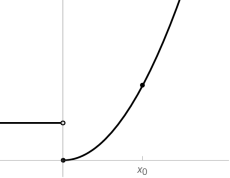
Figure 1. The function in (4.2).

Then $\alpha(x_{0},r)=4$ for $0<r\leq x_{0}$ and $\alpha(x_{0},r)=0$ for $r>x_{0}$. Therefore, Condition $(C^{\prime})$ fails to hold regardless of the choice of $r>0$, but Condition $(C)$ is satisfied for $r=x_{0}$.

Remark 4.3 (Attainment of the minimum).

Assumption $(A^{\prime})$ implies the existence of a global minimiser $x^{\star}$ of $f$ satisfying $\mathsf{d}(x^{\star},x_{0})\leq(\theta\circ f)(x_{0})$ and $f(x^{\star})=0$. This follows from a result by Ioffe [16], which we recall in Lemma 6.1 below. To derive the conclusion, Ioffe’s result should be to be applied to the function $\theta\circ{f}$, and a metric version of the chain rule is required to relate the slope of $f$ to the slope of $\theta\circ{f}$. For completeness, we give a proof of this chain rule in Lemma A.1.

In light of this observation, it is possible to derive results similar to Theorem 1.4 by applying existing results for convergence to a global minimum under the KŁ condition that assume the existence of a global minimum close to the starting point $x_{0}$; see, e.g., [4, Thm. 10] and [5, Thm. 2.12] for such results for discrete schemes. However, a combination of these results with Ioffe’s result yields a non-optimal criterion, as the KŁ inequality is required to hold on a bigger set than necessary. Moreover, some additional assumptions are made in the aforementioned results.

Remark 4.4 (Sharpness of Condition $(A)$).

To guarantee the existence and the proximity of a global minimiser of $f$ under Condition $(A)$, the constant $r$ in the inequality $(\theta\circ f)(x_{0})\leq r$ cannot be replaced by any larger constant.

To see this, fix $M<\infty$ (large) and consider for (small) $\varepsilon\geq 0$ the function $f_{\varepsilon}:[0,\infty)\to[0,\infty)$ defined by $f_{\varepsilon}(x)=\theta^{-1}(x+\varepsilon)$ for $0\leq x<M$ and $f_{\varepsilon}(x)=0$ for $x\geq M$. Fix $x_{0}\in(0,M/2)$. Differentiating the identity $\theta(f_{\varepsilon}(x))=x+\varepsilon$, we find that $(\theta^{\prime}\circ f_{\varepsilon})(x)f^{\prime}_{\varepsilon}(x)=1$ for $0<x<M$. In particular, the second inequality in Condition $(A)$ is satisfied in an open ball of radius $x_{0}$ around $x_{0}$.

If $\varepsilon=0$, the identity $\theta(f_{0}(x_{0}))=x_{0}$ implies that Condition $(A)$ holds with $r=x_{0}$, and indeed, the distance of $x_{0}$ to the nearest global minimiser of $f$ (which is $0$) equals $x_{0}$.

If $\varepsilon>0$, Condition $(A)$ fails to hold just barely (since $\theta(f_{\varepsilon}(x_{0}))=x_{0}+\varepsilon$), but the distance of $x_{0}$ to the nearest global minimiser (which is $M$) is enormous (namely, $M-x_{0}$) and the gradient flow curve starting from $x_{0}$ will converge to $0$, which is not a global minimiser.

The following non-smooth example in ${\mathbb{R}}$ shows that Condition $(A)$ can be applied in a setting where there is no uniqueness of gradient flow curves with a given starting point.

Example 4.5 (Non-uniqueness).

Let $\lambda>0$ and $a>0$, and consider the function $f\colon{\mathbb{R}}\to{\mathbb{R}}$ (see Fig. 2(a))

$$f(x)=\min\bigg{\{}\frac{\lambda}{2}(x-a)^{2},\ \frac{\lambda}{2}(x+a)^{2}\bigg{\}}\,\mathrm{.}$$ (4.3)

This function is everywhere smooth except at the origin. For each $x_{0}\neq 0$, there exists a unique gradient-flow trajectory starting at $x_{0}$, given by $y_{t}\operatorname{\coloneqq}e^{-\lambda t}x_{0}\pm\big{(}1-e^{-\lambda t}\big{)}a$ for $x_{0}\gtrless 0$. However, there are two distinct gradient-flow trajectories $y^{+}$ and $y^{-}$ starting at the origin, given $y^{\pm}_{t}\operatorname{\coloneqq}\pm\big{(}1-e^{-\lambda t}\big{)}a$ for $t\geq 0$.

In spite of this non-uniqueness, we shall verify that this example satisfies our assumptions. Note that $\left\lvert\mathrm{D}^{-}{f}\right\rvert\!(x)=\lambda\big{\lvert}|x|-a\big{\rvert}$ for all $x\in{\mathbb{R}}$. In particular, $f$ has finite slope at $0$, although it is not differentiable. Consequently, $\frac{\left\lvert\mathrm{D}^{-}{f}\right\rvert\!(x)^{2}}{f(x)}=2\lambda$ for all $x\in{\mathbb{R}}$. It follows that Condition ($C$) holds for all $x_{0}\in{\mathbb{R}}$ with $\alpha(x_{0},r)=2\lambda$ (hence Condition $(A)$ holds with $\theta(u)=\sqrt{2u/\lambda}$), provided $r\geq|x_{0}-a|\wedge|x_{0}+a|$. Thus, at every point $x_{0}\in{\mathbb{R}}$, the criterion provides the optimal result, in the sense that it yields the smallest possible ball centered at $x_{0}$ containing each gradient-flow trajectory starting at $x_{0}$.

Remark 4.6 (Restriction to path connected component).

The second inequality in Condition $(A)$ is required to hold for all $y\in B_{r}(x_{0})\cap\{0<f\leq f(x_{0})\}$. However, in the proof of Theorem 1.4, this bound is needed only on the set $G(x_{0},r)$ consisting of all points inside the ball that are reachable by the considered curve of maximal slope starting at $x_{0}$. Therefore, Theorem 1.4 would still hold if one replaces the set $B_{r}(x_{0})\cap\{0<f\leq f(x_{0})\}$ by $G(x_{0},r)$ in the definition in $(A)$. Of course, in practice $G(x_{0},r)$ is often not explicitly known, so this condition might be not easy to check. Instead of $G(x_{0},r)$, one could also consider the path connected component $P(x_{0},r)$ of $x_{0}$ in $B_{r}(x_{0})\cap\{0<f\leq f(x_{0})\}$ and modify the definition of $(A)$ accordingly.

The following modification of Example 4.5 provides an example where it is useful to employ the modified assumption. Let $\lambda>0$ and $a>0$, and consider the function $f\colon{\mathbb{R}}\to{\mathbb{R}}$ (see Fig. 2(b)) given by

$$f(x)=\min\left\{\max\left\{\frac{\lambda}{2}(x-a)^{2},\varepsilon\right\}\ \frac{\lambda}{2}(x+a)^{2}\right\}\,\mathrm{.}$$ (4.4)

For this function, Assumption ($C$) is satisfied for every $x_{0}<0$ and suitable $r>0$ when $\alpha(x_{0},r)$ is defined with $P(x_{0},r)$ in place of $B_{r}(x_{0})\cap\left\{f\leq f(x_{0})\right\}$. However, it is not satisfied for any $x_{0}<0$ yet sufficiently close to $0$ when $\alpha(x_{0},r)$ is defined as in (4.1).

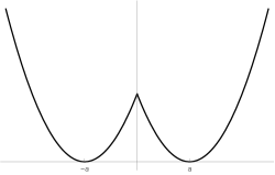
(a) A non-smooth double-well potential (4.3).

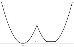
(b) An asymmetric double-well potential (4.4).

Figure 2. The objective functions in Example 4.5 and  Remark 4.6

5. Extension of gradient-flow trajectories

It is possible, even under Condition $(A)$, that a curve of maximal slope defined on a finite interval $[0,T)$ does not extend to a curve of maximal slope on $[0,\infty)$. The following simple example illustrates this phenomenon.

Example 5.1.

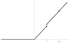
Figure 3. There is no curve of maximal slope with $T=\infty$ starting at $x_{0}$.

For fixed $m,\varepsilon>0$, consider the lower-semicontinuous function $f\colon{\mathbb{R}}\to[0,\infty)$ defined by

$$f(x)=m\,x\,{\bf 1}_{[0,1]}(x)+(mx+\varepsilon){\bf 1}_{(1,\infty)}(x)\,\mathrm{.}$$

See Figure 3. Let $x_{0}>1$ and fix $r>0$. Then $f(x_{0})=mx_{0}+\varepsilon$ and Condition $(A)$ is satisfied with

$$\theta(u)=\frac{2}{m}\sqrt{u(mx_{0}+\varepsilon)}$$

and $r\geq 2(mx_{0}+\varepsilon)/m.$ On the interval $[0,T)$ with $T=\frac{x_{0}-1}{m}$, there exists a unique curve of maximal slope $\left(y_{t}\right)_{t\in[0,T)}$ starting from $x_{0}$. This is the curve which travels at constant speed $m$ towards the discontinuity of $f$, namely $y_{t}=x_{0}-mt$. However, there is no extension of $\left(y_{t}\right)_{t\in[0,T)}$ to a curve of maximal slope defined on $[0,T^{\prime})$ for any $T^{\prime}>T$, since $t\mapsto f(y_{t})$ cannot be (absolutely) continuous on $[0,T^{\prime})$.

Of course, the curve in this example can be naturally extended to $[0,\infty)$ by defining $y_{T}=1$, and concatenating a new curve of maximal slope starting from there. The resulting curve, given by $y_{t}=(x_{0}-mt)_{+}$ for $t\geq 0$, satisfies the exponential convergence rates of Corollary 1.5, even though it is not a curve of maximal slope in the sense of Definition 2.2.

Theorem 5.3 below shows that, under Condition $(A)$, concatenated curves of maximal slope always satisfy the convergence rates of Theorem 1.4. The key ingredient is the following simple observation, which shows that Condition $(A)$ is preserved under curves of maximal slope $(y_{t})_{t\geq 0}$ in a suitable sense: if the condition holds at time $0$ for $x_{0}$ and some $r>0$, then it holds at any time $t\geq 0$ for the point $y_{t}$ and the radius $r-\mathsf{d}(y_{t},y_{0})$ and with the same parameter function $\theta$.

Remark 5.2 (Assumption preserved along the flow).

Suppose that Condition $(A)$ holds for $x_{0}\in\mathrm{dom}(f)$ and $r>0$. Let $\left(y_{t}\right)_{t\in[0,T)}$ be a curve of maximal slope, and extend it to $\left(y_{t}\right)_{t\in[0,T]}$ using Theorem 1.4. Then we have by (3.1) that for $t\in[0,T)$,

$$(\theta\circ f)(y_{t})\leq(\theta\circ f)(x_{0})-\mathsf{d}(x_{0},y_{t})\leq r-\mathsf{d}(x_{0},y_{t}),$$

which implies that Condition $(A)$ holds for $y_{t}$ (in place of $x_{0}$) and $r-\mathsf{d}(x_{0},y_{t})$ (in place of $r$); note that if $f(y_{t})=0$ it is possible that $r-\mathsf{d}(x_{0},y_{t})=0$; otherwise this quantity is strictly positive. If $f$ is lower semicontinuous, then Condition $(A)$ holds also for $y_{T}$ and $r-\mathsf{d}(x_{0},y_{T})$, as can be seen by taking limits.

Theorem 5.3.

Let $f:X\to[0,\infty]$ be a lower semicontinuous function on a complete metric space $(X,\mathsf{d})$ and suppose that $x_{0}\in X$ and $r>0$ satisfy Condition $(A)$ for some parameter function $\theta$. Let $K\geq 1$, $0=T_{0}<T_{1}<\ldots<T_{K}=T\leq\infty$ and $(y_{t})_{t\in[T_{i},T_{i+1})}$ be curves of maximal slope starting from $x_{i}$, where $x_{i}=\lim_{t\uparrow T_{i}}y_{t}\in B_{r}(x_{0})$ for $1\leq i\leq K-1$. Then, setting $t_{*}\coloneqq\inf\left\{t\in[0,T):f(y_{t})=0\right\}\wedge T$, the following assertions hold:

1. $y_{t}\in\overline{B_{r}(x_{0})}$ for all $0\leq t<T$;

2. $y_{T}:=\lim_{t\to T}y_{t}$ exists and belongs to $\overline{B_{r}(x_{0})}$;

3. $\mathsf{d}(y_{s},y_{t})\leq(\theta\circ f)(y_{s})-(\theta\circ f)(y_{t})$ for all $0\leq t\leq T$.

4. for all $0\leq t\leq t_{*}$

   $$\Gamma\big{(}\mathsf{d}(y_{t},y_{T})\big{)} \leq\Gamma(r)-t,$$ (5.1)

   $$(\eta\circ f)(y_{t}) \leq(\eta\circ f)(x_{0})-t.$$ (5.2)

Proof.

i and ii follow from a repeated application of Theorem 1.4 and Remark 5.2.

iii:  Recall first that, for $K=0,\ldots,K-1$ and $T_{k}\leq s\leq t\leq T_{k+1}$, by (1.8)

$$\mathsf{d}(y_{s},y_{t})\leq(\theta\circ f){(y_{s})}-(\theta\circ f){(y_{t})}\,\mathrm{.}$$

Therefore by a telescoping sum argument, the same inequality holds for all $0\leq s\leq t\leq T$.

iv:  If $K=1$, the claim follows from Theorem 1.4. Proceeding by induction, we assume that the claim holds for all $K\leq\bar{K}$. We shall show that it also holds for $K=\bar{K}+1$. For this purpose, suppose that $t_{*}\geq\bar{K}$ and let $T_{\bar{K}}\leq t\leq t_{*}$, otherwise the conclusion is trivial. Then notice that the induction hypothesis yields $(\eta\circ f)(x_{\bar{K}})\leq(\eta\circ f)(x_{0})-T_{\bar{K}}$. Moreover, applying Theorem 1.4 for $(y_{t})_{t\in[T_{\bar{K}},T_{\bar{K}+1}]}$, we find

$$(\eta\circ f)(y_{t})\leq(\eta\circ f)(x_{\bar{K}})-(t-T_{\bar{K}}).$$

Combining these bounds, (5.2) follows. Finally, (5.1) follows from iii and (5.2) in the same way as in the proof of Theorem 1.4. ∎

Remark 5.4.

Theorem 5.3 still holds true if we replace the sub-level set of $f$ in condition $(A)$ with the path-connected component $P(x_{0},r)$ as in Remark 4.6; however the proof does not work if we instead use $G(x_{0},r)$, since, in this case, the inequality $(\theta^{\prime}\circ f)\cdot\left\lvert\mathrm{D}^{-}{f}\right\rvert\!\geq 1$ may not hold on $G\big{(}y_{T_{i}},r-\mathsf{d}(x_{0},y_{T_{i}})\big{)}$.

6. Convergence of the discrete scheme

This section contains the proof of Theorem 1.6, which deals with the convergence of proximal point sequences to a global minimiser. Our proof is based on adaptation of the arguments in [8, Thm. 24]). A key tool is the following result by Ioffe [17]; see also [14, Lemma 2.5].

Lemma 6.1 (Ioffe’s Lemma).

Let $g\colon X\to[-\infty,\infty]$ be a lower semicontinuous functional on a complete metric space $(X,\mathsf{d})$. Let $x\in\mathrm{dom}(g)$ and suppose that there are constants $\delta\leq g(x)$ and $R>0$ such that

$$\left\lvert\mathrm{D}^{-}{g}\right\rvert\!(u) \geq v\quad\text{ for all }u\in B_{R}(x)\cap\left\{\delta<g\leq g(x)\right\}$$

for some $v>(g(x)-\delta)/R$. Then:

$$\mathsf{d}\big{(}{x,\left\{g\leq\delta\right\}}\big{)}\leq\frac{g(x)-\delta}{v}.$$ (6.1)

Throughout the remainder of this section we impose the following standing assumptions that are in force without further mentioning:

• $f\colon X\to[0,\infty]$ is a proper and lower semicontinuous functional on a complete metric space $(X,\mathsf{d})$;

• $x_{0}\in\mathrm{dom}(f)$ and $r>0$ satisfy Condition $(A^{\prime})$ for some parameter function $\theta$;

• there exists a time-step $\bar{\tau}>0$ (that will be fixed from now on) such that, for all $x\in B_{r}(x_{0})\cap\left\{f\leq f(x_{0})\right\}$ and $\tau\in(0,\bar{\tau})$, the functional

  $$X\ni y\longmapsto f(y)+\frac{1}{2\tau}\mathsf{d}(x,y)^{2}$$ (6.2)

  has at least one global minimiser. The non-empty set of minimisers will be denoted by $J_{\tau}(x)$.

The latter condition is satisfied with $\bar{\tau}=\infty$ if $(X,\mathsf{d})$ is proper, i.e., if all closed $\mathsf{d}$-bounded sets in $X$ are compact.

The following result contains some fundamental properties of $J_{\tau}$, which can be found in [1] under slightly different assumptions. The same proofs apply to our setting.

Lemma 6.2.

For $x\in B_{r}(x_{0})\cap\left\{f\leq f(x_{0})\right\}$ the following assertions hold:

$$f(z_{0})\geq f(z_{1}) \text{for all }0<\tau_{0}\leq\tau_{1}<\bar{\tau}\text{ and }z_{0}\in J_{\tau_{0}}(x),z_{1}\in J_{\tau_{1}}(x)\,\mathrm{;}\;\,$$ (6.3)

$$\mathsf{d}(x,z)\geq\tau\left\lvert\mathrm{D}^{-}{f}\right\rvert\!(z) \text{for all }0<\tau<\bar{\tau}\text{ and }z\in J_{\tau}(x)\,\mathrm{;}\;\,$$ (6.4)

$$f(z)+\frac{\mathsf{d}(x,z)^{2}}{2\tau}+\int_{0}^{\tau}\frac{\mathsf{d}(x,z_{s})^{2}}{2s^{2}}\mathop{}\!\mathrm{d}s=f(x) \text{for all }0<\tau<\bar{\tau}\text{ and }z\in J_{\tau}(x),z_{s}\in J_{s}(x)\,\mathrm{.}$$ (6.5)

Proof.

Inequality  (6.3) can be found in [1, Lem. 3.1.2]; (6.4) can be found in [1, Lem. 3.1.3]; (6.5) can be found in [1, Thm. 3.1.4, Eqn. (3.1.12)]. ∎

In the following result we consider a slightly more general notion of proximal point sequences, as we allow the step-size $\tau=\tau_{k}$ to depend on the step $k$. This will be useful in Lemma 6.6 below.

Lemma 6.3 (Confinement and distance bound).

Let $\left(y_{k}\right)_{k=0}^{N}$ with $N\in{\mathbb{N}}$ be a proximal point sequence starting at $x_{0}$ with step-sizes $\tau_{k}\in(0,\bar{\tau})$ for $0\leq k<N$. Then for all $0\leq k\leq\ell\leq N$ we have the distance bound

$$\mathsf{d}(y_{k},y_{\ell})\leq(\theta\circ f)(y_{k})-(\theta\circ f)(y_{\ell}).$$ (6.6)

In particular, $y_{k}\in B_{r}(x_{0})$ for all $0\leq k\leq N$.

Proof.

We will prove that (6.6) holds for all $0\leq i\leq j\leq N$ by induction on $N$, noting that the case $N=0$ is trivial.

We thus suppose that the claim is true for some $N\geq 0$, and let $\left(y_{k}\right)_{k=0}^{N+1}$ be a proximal point sequence starting at $x_{0}$. By the induction hypothesis and the triangle inequality it suffices to prove that $\mathsf{d}(y_{N},y_{N+1})\leq(\theta\circ f)(y_{N})-(\theta\circ f)(y_{N+1})$. If $f(y_{N})=0$, we have $y_{N}=y_{N+1}$ and the claim follows. We thus assume that $f(y_{N})>0$.

By Condition $(A^{\prime})$ there exists $\varepsilon>0$ such that $(1+\varepsilon)(\theta\circ f)(x_{0})<r$. We will apply Lemma 6.1 to

$$g=\theta\circ f,\quad x=y_{N},\quad\delta=(\theta\circ f)(y_{N+1}),\quad R=(1+\varepsilon)(\theta\circ f)(y_{N}),\quad v=1.$$

We will show that the assumptions of Lemma 6.1 are satisfied.

• Firstly, we claim that $\left\lvert\mathrm{D}^{-}{g}\right\rvert\!(u)\geq 1$ for $u\in B_{R}(y_{N})\cap\left\{\delta<g\leq g(y_{N})\right\}$. Indeed, by the triangle inequality and the induction hypothesis,

  $$\mathsf{d}(x_{0},u) \leq\mathsf{d}(x_{0},y_{N})+\mathsf{d}(y_{N},u)$$

  $$\leq\Big{(}(\theta\circ f)(x_{0})-(\theta\circ f)(y_{N})\Big{)}+(1+\varepsilon)(\theta\circ f)(y_{N})$$

  $$=(\theta\circ f)(x_{0})+\varepsilon(\theta\circ f)(y_{N})\leq(1+\varepsilon)(\theta\circ f)(x_{0})<r.$$

  This shows that $u\in B_{r}(x_{0})$. Moreover, since $\theta$ is strictly increasing, $f(u)\leq f(y_{N})\leq f(x_{0})$. Since furthermore $f(u)>0$, Condition $(A^{\prime})$ implies that $\theta^{\prime}(f(u))\left\lvert\mathrm{D}^{-}{f}\right\rvert\!(u)\geq 1$. In particular, $\left\lvert\mathrm{D}^{-}{f}\right\rvert\!(u)>0$, hence $u$ is not an isolated point. Therefore, Lemma A.1 yields the desired inequality

  $$\left\lvert\mathrm{D}^{-}{g}\right\rvert\!(u)=\theta^{\prime}(f(u))\left\lvert\mathrm{D}^{-}{f}\right\rvert\!(u)\geq 1.$$

• Secondly, we claim that $g(y_{N})-\delta<R$. Indeed,

  $$g(y_{N})-\delta=(\theta\circ f)(y_{N})-(\theta\circ f)(y_{N+1})<(1+\varepsilon)(\theta\circ f)(y_{N})=R.$$

Using that $\theta$ is strictly increasing, we deduce from Lemma 6.1 that

$$\mathsf{d}\big{(}y_{N},\big{\{}f\leq f(y_{N+1})\big{\}}\big{)}\leq(\theta\circ f)(y_{N})-(\theta\circ f)(y_{N+1}).$$

This means that for any $\kappa>0$ there exists $\bar{x}\in X$ such that

$$f(\bar{x})\leq f(y_{N+1})\quad{\rm and}\quad\mathsf{d}(\bar{x},y_{N})<(\theta\circ f)(y_{N})-(\theta\circ f)(y_{N+1})+\kappa.$$

On the other hand, since $y_{N+1}\in J_{\tau_{N}}(y_{N})$, we have

$$\mathsf{d}^{2}(y_{N+1},y_{N})\leq 2\tau_{N}\big{(}f(\bar{x})-f(y_{N+1})\big{)}+\mathsf{d}^{2}(\bar{x},y_{N}).$$

As $\kappa>0$ can be chosen arbitrarily small, a combination of these bounds yields

$$\mathsf{d}\big{(}{y_{N},y_{N+1}}\big{)}\leq(\theta\circ f)(y_{N})-(\theta\circ f)(y_{N+1}),$$

which completes the induction step and the proof of (6.6).

The final assertion follows from (6.6) since $\theta(f(x_{0}))<r$ by Condition $(A^{\prime})$ . ∎

Lemma 6.4.

For any $\tau\in(0,\bar{\tau})$ there exists an infinite proximal point sequence $\left(y_{k}\right)_{k\geq 0}$ with $y_{0}=x_{0}$.

Proof.

It suffices to iteratively construct the sequence $\left(y_{k}\right)_{k}$ by letting $y_{0}\operatorname{\coloneqq}x_{0}$ and $y_{k+1}$ be a minimiser in (6.2) with $y_{k}$ in place of $x$, noting that $y_{k}\in B_{r}(x_{0})$ by Lemma 6.3 and $f(y_{k})\leq f(x_{0})$ by (6.5). ∎

Lemma 6.5.

Let $(y_{k})_{k\geq 0}$ be a proximal point sequence and suppose that $y_{\infty}\coloneqq\lim_{k\to\infty}y_{k}$ exists. Then

$$f(y_{\infty})=\lim_{k\to\infty}f(y_{k})\quad{\rm and}\quad\lim_{k\to\infty}\left\lvert\mathrm{D}^{-}{f}\right\rvert\!(y_{k})=0.$$

Proof.

The lower semicontinuity of $f$ yields $f(y_{\infty})\leq\liminf_{k\to\infty}f(y_{k})$. On the other hand, since $y_{k}\in J_{\tau}(y_{k-1})$ we have

$$f(y_{k})\leq f(y_{\infty})+\frac{1}{2\tau}\mathsf{d}(y_{k-1},y_{\infty})^{2},$$

hence $\limsup_{k\to\infty}f(y_{k})\leq f(y_{\infty})$. Combining these inequalities, we obtain the first identity.

As for the second identity, note that

$$0\leq\left\lvert\mathrm{D}^{-}{f}\right\rvert\!(y_{k})\leq\frac{\mathsf{d}(y_{k-1},y_{k})}{\tau}$$

for $k\geq 1$ by (6.4). The conclusion follows by letting $k\to\infty$. ∎

Proof of Theorem 1.6.

Fix $\tau\in(0,\bar{\tau})$. The existence of an infinite proximal point sequence $\left(y_{k}\right)_{k\geq 0}$ with $y_{0}=x_{0}$ and step-size $\tau$ was proved in Lemma 6.4.

Statement i was proved in Lemma 6.3.

The distance bound in iii was proved for $0\leq i\leq j<\infty$ in Lemma 6.3 as well.

To prove ii, note that $(\theta(f(y_{k})))_{k}$ is a Cauchy sequence, as it is non-negative and non-increasing. Therefore, iii implies the Cauchy property of $\left(y_{k}\right)_{k}$ and hence the existence of $y_{\infty}\coloneqq\lim_{k\to\infty}y_{k}$. Using (6.6) and Condition $(A^{\prime})$ we infer for $0\leq i<\infty$ that

$$\mathsf{d}(y_{i},y_{\infty})\leq\liminf_{j\to\infty}\mathsf{d}(y_{i},y_{j})\leq(\theta\circ f)(y_{i})<r.$$

This show that $y_{\infty}\in{B_{r}(x_{0})}$ and the distance bound in iii for $j=\infty$ follows as well. To show that $f(y_{\infty})=0$, we may assume that $f(y_{k})>0$ for all $k$, since otherwise there is nothing to prove. Since $\left\lvert\mathrm{D}^{-}{f}\right\rvert\!(y_{k})\to 0$ as $k\to\infty$ by Lemma 6.5 and

$$\theta^{\prime}(f(y_{k}))\cdot\left\lvert\mathrm{D}^{-}{f}\right\rvert\!(y_{k})\geq 1$$

by Condition $(A^{\prime})$, we infer that $\theta^{\prime}(f(y_{k}))\to\infty$. As $\theta^{\prime}$ is continuous on $(0,\infty)$ and the sequence $(f(y_{k}))_{k}$ is non-increasing, it follows that $f(y_{k})\to 0$, hence $f(y_{\infty})=0$ by lower semicontinuity of $f$. ∎

For specific choices of the parameter function $\theta$ it is possible to obtain more explicit estimates on the decay of $f(y_{k})$ and $\mathsf{d}(y_{k},y_{\infty})$ as $k\to\infty$. We adapt and refine some arguments from [3], where similar results are proved.

Lemma 6.6.

Let $\left(y_{k}\right)_{k=0}^{\infty}$ be a proximal point sequence with step-size $\tau\in(0,\bar{\tau})$ starting at $x_{0}$. If the parameter function $\theta$ is concave, we have, for all $k\geq 0$,

$$f(y_{k})-f(y_{k+1})\geq\frac{\tau}{(\theta^{\prime}\circ f)(y_{k+1})^{2}}\,\mathrm{.}$$ (6.7)

Proof.

Fix $k\geq 0$ and take $z_{s}\in J_{s}(y_{k})$ for $s\in(0,\tau)$. Using De Giorgi’s formula (6.5), the inequality (6.4), and Condition $(A^{\prime})$, we obtain

$$f(y_{k})-f(y_{k+1})=\frac{\mathsf{d}(y_{k},y_{k+1})^{2}}{2\tau}+\int_{0}^{\tau}\frac{\mathsf{d}(y_{k},z_{s})^{2}}{2s^{2}}\mathop{}\!\mathrm{d}s \geq\frac{\tau}{2}\left\lvert\mathrm{D}^{-}{f}\right\rvert\!(y_{k+1})^{2}+\frac{1}{2}\int_{0}^{\tau}{\left\lvert\mathrm{D}^{-}{f}\right\rvert\!(z_{s})^{2}}\mathop{}\!\mathrm{d}s$$

$$\geq\frac{\tau}{2(\theta^{\prime}\circ f)(y_{k+1})^{2}}+\int_{0}^{\tau}\frac{1}{2(\theta^{\prime}\circ f)(z_{s})^{2}}\mathop{}\!\mathrm{d}s\,\mathrm{.}$$

Note that Condition $(A^{\prime})$ can be applied to $z_{s}$ since $f(z_{s})\leq f(y_{k})\leq f(x_{0})$ and Lemma 6.3 implies that $z_{s}\in B_{r}(x_{0})$. Since $\theta$ is concave and $f(z_{s})\geq f(y_{k+1})$ by (6.3), the result follows. ∎

Note that a weaker decay estimate with an additional factor of $1/2$ in the right-hand side of (6.7) can be obtained without using De Giorgi’s identity (6.5).

Corollary 6.7.

Suppose that the parameter function $\theta$ is given by $\theta(u)=\frac{c}{\gamma}u^{\gamma}$ for some $c>0$ and $\gamma\in(0,1]$. Let $\left(y_{k}\right)_{k\geq 0}$ be a proximal point sequence starting at $x_{0}$ with step-size $\tau\in(0,\bar{\tau})$, and set $y_{\infty}:=\lim_{k\to\infty}y_{k}$. The following assertions hold:

1. If $\gamma=1$, then $y_{k}=y_{\infty}$ and $f(y_{k})=0$ for all $k\geq\lceil cr/\tau\rceil$.

2. If $\frac{1}{2}<\gamma<1$, then, for $k\geq 0$,

   $$f(y_{k}) \leq\left(1+\frac{\tau}{c^{2}}f(x_{0})^{1-2\gamma}\right)^{-k}f(x_{0})\,\mathrm{,}\;\,$$

   $$\mathsf{d}(y_{k},y_{\infty}) \leq\frac{c}{\gamma}f(y_{k})^{\gamma}=\mathcal{O}\left(\left(1+\frac{\tau}{c^{2}}f(x_{0})^{1-2\gamma\color[rgb]{0,0,0}}\right)^{-k\gamma}\right)\,\mathrm{,}\;\,$$

   and, for $k\geq k_{0}\coloneqq\log_{1+\tilde{\alpha}}\left(2\tilde{\alpha}^{-{1}/{(2\gamma-1)}}\right)$ with $\tilde{\alpha}\coloneqq\frac{\tau}{c^{2}}f(x_{0})^{1-2\gamma}$,

   $$f(y_{k}) \leq\Big{(}\frac{\tau}{c^{2}}\Big{)}^{\frac{1}{2\gamma-1}}2^{-(2-2\gamma)^{-(k-k_{0})}}\,\mathrm{,}\;\,$$

   $$\mathsf{d}(y_{k},y_{\infty}) \leq\frac{c}{\gamma}f(y_{k})^{\gamma}=\mathcal{O}\left({2^{-\gamma\left(2-2\gamma\right)^{-(k-k_{0})}}}\right)\,\mathrm{.}$$

3. If $\gamma=\frac{1}{2}$ then, for $k\geq 0$,

   $$f(y_{k}) \leq\left(1+\frac{\tau}{c^{2}}\right)^{-k}f(x_{0})\,\mathrm{,}\;\,$$

   $$\mathsf{d}(y_{k},y_{\infty}) \leq 2c\sqrt{f(y_{k})}\leq 2c\left(1+\frac{\tau}{c^{2}}\right)^{-k/2}\sqrt{f(x_{0})}\,\mathrm{.}$$

4. If $0<\gamma<\frac{1}{2}$ then, for $k\geq 0$,

   $$f(y_{k}) \leq\Big{(}f(x_{0})^{-(1-2\gamma)}+C_{1}k\Big{)}^{-\frac{1}{1-2\gamma}}=\mathcal{O}\big{(}k^{-\frac{1}{1-2\gamma}}\big{)},$$

   $$\mathsf{d}(y_{k},y_{\infty}) \leq\frac{c}{\gamma}f(y_{k})^{\gamma}=\mathcal{O}\big{(}{k^{-\frac{\gamma}{1-2\gamma}}}\big{)},$$

   where $C_{1}=\sup_{R>1}\min\big{\{}\tfrac{\tau(1-2\gamma)}{c^{2}R},\big{(}{R^{\frac{1-2\gamma}{2-2\gamma}}-1}\big{)}f(x_{0})^{2\gamma-1}\big{\}}$.

Proof.

$(i)$:  Suppose that $f(y_{K})>0$ for some $K\geq 0$. Condition $(A^{\prime})$ yields $\left\lvert\mathrm{D}^{-}{f}\right\rvert\!(y_{k})\geq\frac{1}{c}$ for all $0\leq k\leq K$, hence $\mathsf{d}(y_{k},y_{k+1})\geq\frac{\tau}{c}$ for all $0\leq k\leq K-1$ by (6.4). Using Condition $(A^{\prime})$ and Lemma 6.3 we infer that

$$r>c(f(x_{0})-f(y_{K}))=c\sum_{k=0}^{K-1}\Big{(}f(y_{k})-f(y_{k+1})\Big{)}\geq\sum_{k=0}^{K-1}d(y_{k},y_{k+1})\geq\frac{K\tau}{c},$$

hence $K<cr/\tau$. It follows that $f(y_{k})=0$ and therefore $y_{k}=y_{\infty}$ for all $k\geq\lceil cr/\tau\rceil$.

$(ii)-(iv)$:  Write $f_{k}\coloneqq f(y_{k})$. From $\eqref{eq:one-step-decay-concave}$ we deduce the recursive inequality

$$f_{k-1}-f_{k}\geq\frac{\tau}{c^{2}}f_{k}^{2-2\gamma}\,\mathrm{.}$$

This inequality yields the decay of $f_{k}$ using Lemma B.1 with $\alpha={\tau}/{c^{2}}$ and $\delta=2-2\gamma$. The decay estimates for $d_{k}\coloneqq\mathsf{d}(y_{k},y_{\infty})$ follow from the bounds for $f_{k}$ combined with Theorem 1.6iii. ∎

Remark 6.8.

In general — unlike in the continuous setting of Corollary 3.8 — the discrete scheme does not converge in a finite number of steps when $\frac{1}{2}<\gamma<1$. For suitable $f\in C^{1}({\mathbb{R}}^{n})$, this is easy to deduce from the equivalent formulation in (1.3). However, the corollary above shows that the rate of convergence is (asymptotically) faster than exponential.

Example 6.9 (Non-uniqueness revisited).

Let us consider again the function $f$ defined in (4.3) (see Fig. 2(a)) and let $\tau>0$. For any $x_{0}\neq 0$, the resolvent $J_{\tau}(x_{0})$ is single-valued. However, if $x_{0}=0$, the resolvent $J_{\tau}(x_{0})$ contains two elements, say $x_{\tau}$ and $-x_{\tau}$. Consequently, there are two distinct proximal point sequences starting at $x_{0}=0$; once $x_{\tau}^{1}\in J_{\tau}(x_{0})$ is selected, the rest of the sequence is determined. Corollary 1.7 implies the exponential convergence for both of these sequences.

Appendix A A nonsmooth chain rule

In practice, it can be difficult to compute the slope of a non differentiable function, because tools such as the chain rule are missing. We have however the following basic substitute Lemma.

Lemma A.1.

Let $f\colon X\to(-\infty,\infty]$ be proper and lower semicontinuous and let $g\colon{\mathbb{R}}\to{\mathbb{R}}$ be lower semicontinuous and non-decreasing. Then $g\circ f\colon X\to(-\infty,\infty]$ is proper and lower semicontinuous. Furthermore, if $x\in\mathrm{dom}(f)$ is not isolated and is such that there exists the left derivative $\partial_{-}g\left(f(x)\right)\geq 0$ of $g$ at $f(x)$, then

$$\left\lvert\mathrm{D}^{-}{(g\circ f)}\right\rvert\!(x)=\partial_{-}g\left(f(x)\right)\cdot\left\lvert\mathrm{D}^{-}{f}\right\rvert\!(x)\,\mathrm{.}$$ (A.1)

Proof.

The lower semicontinuity of $g\circ f$ is well known, so we only prove (A.1). Set

$$S\coloneqq\left\{\left(y_{n}\right)_{n}\subset X:y_{n}\to x\,\mathrm{,}\;\,y_{n}\neq x\right\}.$$

Since $x$ is not isolated, $S\neq\varnothing$. For a function $h\colon X\to(-\infty,\infty]$ we have

$$\limsup_{y\to x}h(y)=\sup\left\{\limsup_{n\to\infty}\>h(y_{n}):\left(y_{n}\right)_{n}\in S\right\}=\max\left\{\limsup_{n\to\infty}\>h(y_{n}):\left(y_{n}\right)_{n}\in S\right\}.$$ (A.2)

We first prove that

$$\left\lvert\mathrm{D}^{-}{(g\circ f)}\right\rvert\!(x)\leq\partial_{-}g\left(f(x)\right)\cdot\left\lvert\mathrm{D}^{-}{f}\right\rvert\!(x)\,\mathrm{.}$$ (A.3)

Let $\left(y_{n}\right)_{n}\in S$. We need to show that

$$\limsup_{n\to\infty}\frac{\left[(g\circ f)(y_{n})-(g\circ f)(x)\right]_{-}}{\mathsf{d}(y_{n},x)}\leq\partial_{-}g\left(f(x)\right)\cdot\left\lvert\mathrm{D}^{-}{f}\right\rvert\!(x)\,\mathrm{.}$$

Observe that if $f(y_{n})\geq f(x)$ then, since $g$ is non decreasing,

$$\frac{\left[(g\circ f)(y_{n})-(g\circ f)(x)\right]_{-}}{\mathsf{d}(y_{n},x)}=0\,\mathrm{.}$$

Therefore without loss of generality (by changing sequence and/or restricting to a subsequence) we can assume that $f(y_{n})<f(x)$. Then, passing to the limit superior as $n\to\infty$ we see that $\limsup_{n}f(y_{n})\leq f(x)$. By lower semicontinuity of $f$ we have as well that $\liminf_{n}f(y_{n})\geq f(x)$, thus there exists $\lim_{n}f(y_{n})=f(x)$. Noting also that

$$\frac{\left[(g\circ f)(y_{n})-(g\circ f)(x)\right]_{-}}{\mathsf{d}(y_{n},x)} =\frac{\big{[}(g\circ f)(y_{n})-(g\circ f)(x)\big{]}_{-}}{\big{[}f(y_{n})-f(x)\big{]}_{-}}\cdot\frac{\big{[}f(y_{n})-f(x)\big{]}_{-}}{\mathsf{d}(y_{n},x)}$$ (A.4)

$$=\frac{g(f(x))-g(f(y_{n}))}{f(x)-f(y_{n})}\cdot\frac{\left[f(y_{n})-f(x)\right]_{-}}{\mathsf{d}(y_{n},x)}$$

we conclude that

$$\limsup_{n\to\infty}\frac{\big{[}(g\circ f)(y_{n})-(g\circ f)(x)\big{]}_{-}}{\mathsf{d}(y_{n},x)}\leq\partial_{-}g\left(f(x)\right)\cdot\left\lvert\mathrm{D}^{-}{f}\right\rvert\!(x)$$

as desired.

We now prove the converse inequality:

$$\left\lvert\mathrm{D}^{-}{(g\circ f)}\right\rvert\!{(x)}\geq\partial_{-}g\left(f(x)\right)\cdot\left\lvert\mathrm{D}^{-}{f}\right\rvert\!(x)\,\mathrm{.}$$ (A.5)

If $\left\lvert\mathrm{D}^{-}{f}\right\rvert\!(x)=0$ the claim is trivial, so we assume now that $\left\lvert\mathrm{D}^{-}{f}\right\rvert\!(x)>0$. By (A.2) there exists $\left(y_{n}\right)_{n}\in S$ such that

$$\limsup_{n\to\infty}\frac{\big{[}f(y_{n})-f(x)\big{]}_{-}}{\mathsf{d}(y_{n},x)}=\left\lvert\mathrm{D}^{-}{f}\right\rvert\!(x)>0\,\mathrm{.}$$

By restricting to a subsequence we can assume that $f(y_{n})<f(x)$. Arguing as before we have the existence of $\lim_{n}f(y_{n})=f(x)$ and that (A.4) holds. Taking the limit superior as $n\to\infty$ in (A.4) gives

$$\left\lvert\mathrm{D}^{-}{(g\circ f)}\right\rvert\!(x)\geq\limsup_{n\to\infty}\frac{\left[(g\circ f)(y_{n})-(g\circ f)(x)\right]_{-}}{\mathsf{d}(y_{n},x)}\geq\partial_{-}g\left(f(x)\right)\cdot\left\lvert\mathrm{D}^{-}{f}\right\rvert\!(x)$$

as desired. Combing (A.5) with the opposite inequality (A.3) yields the assertion. ∎

Appendix B Estimating recursive inequalities

The following lemma contains some estimates that are used in the proof of Corollary 6.7.

Lemma B.1.

Let $\left(f_{k}\right)_{k\in{\mathbb{N}}}$ be a sequence of non-negative real numbers with $f_{0}>0$ and suppose that for some $\alpha,\delta>0$ the recursive relation

$$f_{k-1}-f_{k}\geq\alpha f_{k}^{\delta}$$ (B.1)

holds for all $k\geq 1$. Then, for all $k\geq 0$:

$$f_{k}\leq \big{(}f_{0}^{-(\delta-1)}+Ck\big{)}^{-1/(\delta-1)} \delta>1\,\mathrm{,}\;\,$$ if (B.2a)

$$f_{k}\leq (1+\alpha)^{-k}f_{0} \delta=1\,\mathrm{,}\;\,$$ if (B.2b)

$$f_{k}\leq \left(1+\tilde{\alpha}\right)^{-k}f_{0} \delta<1\,\mathrm{,}\;\,$$ if (B.2c)

where $\tilde{\alpha}={\alpha}/{f_{0}^{1-\delta}}$ and

$$C\coloneqq\sup_{R>1}\min\left\{\frac{\alpha(\delta-1)}{R},\left(R^{(\delta-1)/\delta}-1\right)f_{0}^{1-\delta}\right\}\,\mathrm{.}$$

Furthermore, if $\delta<1$, we also have

$$f_{k}\leq\alpha^{{1}/{(1-\delta)}}\cdot{2^{-\delta^{-(k-k_{0})}}}\quad\text{for \ }k\geq k_{0}\coloneqq\log_{1+\tilde{\alpha}}\left(2\tilde{\alpha}^{-{1}/{(1-\delta)}}\right)\,\mathrm{.}$$ (B.3)

Proof.

Note first that in all cases the sequence $\left(f_{k}\right)_{k}$ is non-increasing.

(B.2a):  We follow the arguments of [3]. Fix $R\in(1,\infty)$ and consider the concave function $H(s)=\frac{1}{1-\delta}s^{1-\delta}$ and its derivative $h(s)=H^{\prime}(s)=s^{-\delta}$. Observe that (B.1) can be equivalently written as

$$\alpha\leq\left(f_{k-1}-f_{k}\right)h(f_{k})\,\mathrm{.}$$

Suppose first that $h(f_{k})\leq Rh(f_{k-1})$. Using the concavity of $H$ we obtain

$$\alpha \leq\left(f_{k-1}-f_{k}\right)h(f_{k})\leq R\left(f_{k-1}-f_{k}\right)h(f_{k-1})\leq R\left(H(f_{k-1})-H(f_{k})\right)=\frac{R}{\delta-1}\left(f_{k}^{1-\delta}-f_{k-1}^{1-\delta}\right).$$

Writing $C_{1}(R)\coloneqq{\alpha(\delta-1)}/{R}>0$, this shows that

$$f_{k}^{1-\delta}-f_{k-1}^{1-\delta}\geq C_{1}(R)\,\mathrm{.}$$

Suppose next that instead $h(f_{k})>Rh(f_{k-1})$. Raising this inequality to the power $\frac{\delta-1}{\delta}$ we obtain

$$f_{k}^{1-\delta}>R^{\frac{\delta-1}{\delta}}f_{k-1}^{1-\delta}$$

and hence, since $(f_{k})_{k}$ is non-increasing,

$$f_{k}^{1-\delta}-f_{k-1}^{1-\delta} \geq\left(R^{\frac{\delta-1}{\delta}}-1\right)f_{k-1}^{1-\delta}\geq\left(R^{\frac{\delta-1}{\delta}}-1\right)f_{0}^{1-\delta}\eqqcolon C_{2}(R)>0.$$

Finally, defining $C\coloneqq\sup_{R\in(1,\infty)}\min\{C_{1}(R),C_{2}(R)\}>0$, the above inequalities combined yield

$$f_{k}^{1-\delta}-f_{k-1}^{1-\delta}\geq C.$$

Evaluating a telescopic sum, we obtain $f_{k}^{1-\delta}-f_{0}^{1-\delta}\geq Ck$. Rearranging terms we obtain the desired inequality (B.2a).

(B.2b):  This is straightforward.

(B.2c):  Suppose without loss of generality that $f_{k}>0$. From (B.1) it follows that

$$\frac{f_{k-1}}{f_{k}}\geq 1+\frac{\alpha}{f_{k}^{1-\delta}}\geq 1+\frac{\alpha}{f_{0}^{1-\delta}}=1+\tilde{\alpha},$$

from which we deduce (B.2c).

(B.3):  Writing $\tilde{f}_{k}\coloneqq{\alpha^{-1/(1-\delta)}}f_{k}$ we note that (B.1) implies $\tilde{f}_{k}^{\delta}\leq\tilde{f}_{k-1}$ and therefore

$$\tilde{f_{k}}\leq\big{(}\tilde{f}_{k_{0}}\big{)}^{{\delta^{-(k-k_{0})}}}\,\mathrm{.}$$

Moreover, (B.2c) and the definition of $k_{0}$ yield $\tilde{f}_{k_{0}}\leq(1+\tilde{\alpha})^{-k_{0}}\tilde{f}_{0}=\frac{1}{2}$. Combining these estimates, we obtain the desired estimate $\tilde{f_{k}}\leq 2^{-{\delta^{-(k-k_{0})}}}$. ∎

References

- [1] L. Ambrosio, N. Gigli, and G. Savaré. Gradient Flows in Metric Spaces and in the Space of Probability Measures. Lectures in Mathematics - ETH Zürich. Birkhäuser, edition, 2008.
- [2] L. Ambrosio, N. Gigli, and G. Savaré. Calculus and heat flow in metric measure spaces and applications to spaces with Ricci bounds from below. Invent. Math., 395:289–391, 2014.
- [3] H. Attouch and J. Bolte. On the convergence of the proximal algorithm for nonsmooth functions involving analytic features. Math. Program., 116(1-2 (B)):5–16, 2009.
- [4] H. Attouch, J. Bolte, P. Redont, and A. Soubeyran. Proximal alternating minimization and projection methods for nonconvex problems: an approach based on the Kurdyka-Łojasiewicz inequality. Math. Oper. Res., 35(2):438–457, 2010.
- [5] H. Attouch, J. Bolte, and B. F. Svaiter. Convergence of descent methods for semi-algebraic and tame problems: proximal algorithms, forward-backward splitting, and regularized Gauss-Seidel methods. Math. Program., 137(1-2 (A)):91–129, 2013.
- [6] P. L. Bartlett, A. Montanari, and A. Rakhlin. Deep learning: a statistical viewpoint. Acta Numer., 30:87–201, 2021.
- [7] A. Blanchet and J. Bolte. A family of functional inequalities: Łojasiewicz inequalities and displacement convex functions. J. Funct. Anal., 275(7):1650–1673, 2018.
- [8] J. Bolte, A. Daniilidis, O. Ley, and L. Mazet. Characterizations of Łojasiewicz inequalities: subgradient flows, talweg, convexity. Trans. Am. Math. Soc., 362(6):3319–3363, 2010.
- [9] J. Bolte, L. Miclo, and S. Villeneuve. Swarm gradient dynamics for global optimization: the density case. arXiv:2204.01306, 2022.
- [10] S. Bombari, M. H. Amani, and M. Mondelli. Memorization and optimization in deep neural networks with minimum over-parameterization. In Advances in Neural Information Processing Systems (NeurIPS), 35:7628–7640, 2022.
- [11] E. Boursier, L. Pillaud-Vivien, and N. Flammarion. Gradient flow dynamics of shallow ReLU networks for square loss and orthogonal inputs. arXiv:2206.00939, 2022.
- [12] S. Chatterjee. Convergence of gradient descent for deep neural networks. arXiv:2203.16462, 2022.
- [13] J. Dolbeault, B. Nazaret, and G. Savaré. A new class of transport distances between measures. Calc. Var. Partial Differential Equations, 34(2):193–231, 2009.
- [14] D. Drusvyatskiy, A. D. Ioffe, and A. S. Lewis. Curves of descent. SIAM J. Control Optim., 53(1):114–138, 2015.
- [15] D. Hauer and J. M. Mazón. Kurdyka-Łojasiewicz-Simon inequality for gradient flows in metric spaces. Trans. Am. Math. Soc., 372(7):4917–4976, 2019.
- [16] A. D. Ioffe. On Lower Semicontinuity of Integral Functionals. I. SIAM Journal on Control and Optimization, 15(4):521–538, jul 1977.
- [17] A. D. Ioffe. Metric regularity and subdifferential calculus. Russ. Math. Surv., 55(3):501–558, 2000.
- [18] R. Jordan, D. Kinderlehrer, and F. Otto. The Variational Formulation of the Fokker-Planck Equation. SIAM J. Math. Anal., 29:1–17, 1998.
- [19] H. Karimi, J. Nutini, and M. Schmidt. Linear convergence of gradient and proximal-gradient methods under the polyak-łojasiewicz condition. In Machine Learning and Knowledge Discovery in Databases, pages 795–811, Cham, 2016. Springer International Publishing.
- [20] S. Kondratyev and D. Vorotnikov. Spherical Hellinger–Kantorovich Gradient Flows. SIAM J. Math. Anal., 51(3):2053–2084, 2019.
- [21] K. Kurdyka. On gradients of functions definable in o-minimal structures. Ann. Inst. Fourier, 48(3):769–783, 1998.
- [22] L. Liu, M. B. Majka, and Ł. Szpruch. Polyak-Łojasiewicz inequality on the space of measures and convergence of mean-field birth-death processes. Appl. Math. Optim., 87: no. 48, 2023.
- [23] S. Łojasiewicz. A topological property of real analytic subsets. In Equ. Derivees partielles, Paris 1962, Colloques internat. Centre nat. Rech. sci., volume 117, pages 87–89, 1963.
- [24] S. Łojasiewicz. Sur la géométrie semi- et sous- analytique. Ann. I. Fourier, 43(5):1575–1595, 1993.
- [25] J. Maas. Gradient flows of the entropy for finite Markov chains. J. Funct. Anal., 261(8):2250–2292, oct 2011.
- [26] B. Martinet. Régularisation d’inéquations variationnelles par approximations successives. Rev. Franç. Inform. Rech. Opér., 4(R-3):154–158, 1970.
- [27] A. Mielke. A gradient structure for reaction-diffusion systems and for energy-drift-diffusion systems. Nonlinearity, 24(4):1329–1346, 2011.
- [28] M. Muratori and G. Savaré. Gradient flows and evolution variational inequalities in metric spaces. I: Structural properties. J. Funct. Anal., 278(4):108347, 67, 2020.
- [29] S. Oymak and M. Soltanolkotabi. Overparameterized nonlinear learning: Gradient descent takes the shortest path? In K. Chaudhuri and R. Salakhutdinov, editors, Proceedings of the 36th International Conference on Machine Learning, volume 97 of Proceedings of Machine Learning Research, pages 4951–4960. PMLR, 09–15 Jun 2019.
- [30] B. Polyak. Gradient methods for the minimisation of functionals. USSR Computational Mathematics and Mathematical Physics, 3(4):864–878, 1963.
- [31] R. T. Rockafellar. Monotone operators and the proximal point algorithm. SIAM Journal on Control and Optimization, 14(5):877–898, 1976.
- [32] L. Simon. Asymptotics for a class of non-linear evolution equations, with applications to geometric problems. Ann. Math. (2), 118:525–571, 1983.