BanditQ: Fair Multi-Armed Bandits with Guaranteed Rewards per Arm

Abstract

Classic no-regret online prediction algorithms, including variants of the Upper Confidence Bound (UCB) algorithm, Hedge, and EXP3, are inherently unfair by design. The unfairness stems from their very objective of playing the most rewarding arm as many times as possible while ignoring the less rewarding ones among $N$ arms. In this paper, we consider a fair prediction problem in the stochastic setting with hard lower bounds on the rate of accrual of rewards for a set of arms. We study the problem in both full and bandit feedback settings. Using queueing-theoretic techniques in conjunction with adversarial learning, we propose a new online prediction policy called BanditQ that achieves the target reward rates while achieving a regret and target rate violation penalty of $O(T^{\nicefrac{{3}}{{4}}}).$ In the full-information setting, the regret bound can be further improved to $O(\sqrt{T})$ when considering the average regret over the entire horizon of length $T$. The proposed policy is efficient and admits a black-box reduction from the fair prediction problem to the standard MAB problem with a carefully defined sequence of rewards. The design and analysis of the BanditQ policy involve a novel use of the potential function method in conjunction with scale-free second-order regret bounds and a new self-bounding inequality for the reward gradients, which are of independent interest.

1 Introduction

A vast majority of the Multi-armed Bandit (MAB) algorithms deployed in practice are designed to maximize the cumulative rewards (e.g., the number of clicks on ads). Consequently, they could end up discriminating against a subset of arms (which could represent e.g., users belonging to certain categories) the algorithm finds less rewarding (Sweeney, 2013). In a typical case of algorithmic discrimination, Facebook was sued for targeting ads on housing, credit and employment by race, gender, and religion - all protected classes under US law (Hao, 2019). A similar problem of fair allocation of resources arises in wireless settings, where schedulers maximizing the total throughput could result in not serving a subset of users having relatively poor channels. As we discuss below, a number of papers have proposed a solution to the fairness problem by guaranteeing a minimum frequency of pulls of each arm. However, in many problems of practical interest, one is primarily interested in guaranteeing a minimum rate of reward accrual for each arm - not just a minimum frequency at which the arms are to be pulled. For example, in online ad allocation, the advertisers are interested in maximizing the click-through rates rather than the number of times their ad was displayed on a webpage. In wireless scheduling problems, the users are primarily interested in guaranteed data rates (in Mbps) across a time horizon rather than the number of times they are scheduled - a low-level metric transparent to the users. In online crowd sourcing platforms, workers are primarily interested in the amount of money they make over a given span of time compared to the number of times they are assigned a job. Clearly, the rate of reward accruals depends on the unknown reward distribution, which needs to be learned along the way. In this paper, we solve this fair prediction problem in the stochastic setting through a black-box reduction to an adversarial MAB problem by making use of a natural queueing dynamics. Although we consider stochastic i.i.d. rewards, we will see in the sequel that the use of adversarial MAB algorithms is essential to account for the target reward rate constraints.

1.1 Related Works

There is a vast literature on the classic Multi-armed Bandits problem, where the objective is to sequentially pull an arm at each round from a given set of arms of unknown qualities to maximize the cumulative reward at the end of a time horizon. With the bandit feedback of observed rewards, the problem involves an exploration vs exploitation trade-off. See Cesa-Bianchi and Lugosi (2006); Bubeck et al. (2012); Lattimore and Szepesvári (2020) for text-book treatments on MAB. The fair prediction problem belongs to a class of MAB problems with global constraints. Several authors have considered variants of the fair prediction problem in MAB with different definitions for fairness (Joseph et al., 2016; Gillen et al., 2018; Bechavod et al., 2020; Hossain et al., 2021; Huang et al., 2022). Closer to our setting, the papers by Patil et al. (2021); Claure et al. (2020), and Li et al. (2019) considered a stochastic MAB problem while requiring the minimum fraction of pulls of each arm to exceed a given threshold. Celis et al. (2019) considered a similar problem in the personalized recommendation setting where both the minimum and the maximum fraction of pulls are constrained in order to avoid polarization of views. Technically, Li et al. (2019) used a virtual queueing recursion to handle the fairness constraints. However, their UCB-based policy yielded a regret bound which varies linearly with the horizon length (Li et al., 2019, Theorem 2). Chen et al. (2020) considered the above problem in the contextual bandit setting and proposed a no-regret policy with a known context distribution. Cai et al. (2018) considered a related stochastic MAB problem with a long-term constraint on an auxiliary (level-$2$) reward process which is assumed to be independent of the main (level-$1$) rewards of the arms. On the other hand, in our problem, the so-called level-$1$ and level-$2$ reward processes are identical, and hence, these results do not apply. Constrained bandit problems have also been studied in contexts other than fairness as well. Badanidiyuru et al. (2018); Immorlica et al. (2022), and Xia et al. (2015) considered a related Bandits with Knapsack (BwK) problem in stochastic and adversarial environments. In this problem, a given resource budget is allocated to the arms at the beginning, and the game continues until one of the arms finishes all of its budgets. Immorlica et al. (2022) used a Lagrangian-based technique to propose a no-regret policy for the BwK problem. Similar to ours, they also employed an adversarial bandit policy in the stochastic setting.

1.2 Our contributions

In contrast with a major line of work in the literature on fair MABs, which is mainly concerned with guaranteeing a minimum fraction of pulls for each arm, in this paper, we initiate the study of a class of problems guaranteeing a minimum rate of reward accruals for each arm. Compared to the standard MAB problem, here the difficulty stems from the fact that in addition to pulling the unknown best arm sufficiently many times, other arms with unknown mean rewards also need to be pulled frequently enough so as to satisfy the given fairness constraints. Consequently, our proposed algorithm and its analysis are very different from that of the prior works. In particular, we claim the following major contributions in this paper:

1. We propose an online fair prediction policy, called BanditQ, via a black-box reduction to the standard adversarial MAB problem. The proposed BanditQ policy keeps track of the global reward rate constraints with the help of an auxiliary queueing process, which is used to define the rewards for the standard MAB problem.

2. On the technical side, we critically use second-order regret bounds to design no-regret online prediction policies with long-term constraints. The key to our result is a new self-bounding inequality that implicitly controls the growth of the reward gradients (see Eqs. (14) and (19)). The techniques introduced in this paper could be useful for analyzing other constrained sequential learning problems as well.

3. We complement our theoretical results with illustrative numerical simulations.

2 Problem Formulation

We consider an online prediction problem in the stochastic setting with an additional fairness constraint that requires that each arm belonging to a given subset $\mathcal{P}$ (called protected class) must attain pre-specified reward accrual rates, assumed to be feasible. Formally, let there be a set of $N$ arms, which on round $t$ receives a reward vector $\bm{r}(t)\in[0,1]^{N}.$ We consider a stochastic setting where the rewards $\bm{r}(t)$ are generated i.i.d. with an unknown expectation vector $\bm{\mu}.$ On round $t$, an online policy causally predicts a probability distribution $\bm{x}(t)\in\Delta_{N},$ where $\Delta_{N}$ is the set of all probability vectors on $N$ arms. The algorithm then randomly samples an arm $I_{t}\in[N]$ from the distribution $\bm{x}(t)$. Depending on the feedback structure, either the entire reward vector $\bm{r}(t)$ (in the case of full-information) or the reward of the sampled arm $r_{I_{t}}(t)$ (in the case of bandit feedback) is fed to back to the policy at the end of round $t$. The above process continues for a given time horizon of length $T$.

Fairness constraints:

Due to the action of the policy, the selected arm $I_{t}$ receives a random reward of value $r_{I_{t}}(t).$ Hence, if on round $t$, the prediction policy selects arms according to the distribution $\bm{x}(t)$, the $i$^th arm receives a (conditional) expected reward of $x_{i}(t)\mathbb{E}r_{i}(t)=x_{i}(t)\mu_{i},$ and the online policy receives an overall (conditional) expected reward of $\langle\bm{x}(t),\bm{\mu}\rangle.$ Let $\bm{\vec{\lambda}}$ be a given vector of target reward rates. Our fairness constraint requires that the long-term rate of rewards accrued by arm $i\in\mathcal{P}$ must be at least $\lambda_{i},\forall i\in\mathcal{P}.$ We may assume $\lambda_{i}=0,\forall i\in[N]\setminus\mathcal{P}.$

Offline Benchmark and Performance Metric:

We compare the performance of an online policy against any fixed prediction distribution $\bm{x}^{*}\in\Delta_{N}$ that meets the target reward rates. In other words, our comparator class, denoted by the set $\Omega\subseteq\Delta_{N},$ is defined as follows:

$$\Omega(\bm{\vec{\lambda}})=\{\bm{x}^{*}\subseteq\Delta_{N}:x_{i}^{*}\mu_{i}\geq\lambda_{i},~{}\forall i,~{}\textrm{and}~{}\sum_{i}x_{i}^{*}=1,~{}\bm{x}^{*}\geq\bm{0}\}.$$ (1)

Hence, in order for the rate vector $\bm{\vec{\lambda}}$ to be feasible (i.e., $\Omega(\bm{\vec{\lambda}})\neq\emptyset$) it is necessary and sufficient that

$$\sum_{i}\frac{\lambda_{i}}{\mu_{i}}\leq 1.$$ (2)

See Section 7.1 in the Appendix for a brief discussion on the feasibility assumption. The set of all offline benchmarks $\Omega(\bm{\vec{\lambda}})$ is closed and convex with a Euclidean diameter of $D=\sqrt{2}.$ Our goal is to design a prediction policy $\{\bm{x}(t)\}_{t\geq 1}$ that achieves a sublinear (pseudo)-regret against any $\bm{x}^{*}\in\Omega,$ where

$$\textrm{Regret}_{T}(\bm{x}^{*})\equiv\langle\bm{x}^{*},\bm{\mu}\rangle T-\mathbb{E}\sum_{t=1}^{T}\langle\bm{x}(t),\bm{r}(t)\rangle,$$ (3)

while meeting the long-term reward rate constraints that we formalize next. Formally, for any time interval $\mathcal{I}\subseteq[T]$, the asymptotic rate constraint requires:

$$\liminf_{|\mathcal{I}|\to\infty}|\mathcal{I}|^{-1}\mathbb{E}\big{[}\sum_{t\in\mathcal{I}}r_{i}(t)x_{i}(t)\big{]}\geq\lambda_{i},~{}\forall i\in\mathcal{P}.$$ (4)

Note that Eq. (4) requires the minimum reward rate guarantee to hold uniformly across the time horizon for any sufficiently long interval of time. In other words, we require that no individual arm is starved for a long period of time - a problem left open by Patil et al. (2021). Furthermore, following Cai et al. (2018), we also define a non-asymptotic rate violation penalty as follows:

$$\mathbb{V}(T)=\max_{i\in\mathcal{P}}\mathbb{E}\big{[}\sum_{t=1}^{T}\big{(}\lambda_{i}-r_{i}(t)x_{i}(t)\big{)}\big{]}.$$ (5)

In brief, we seek an online prediction policy for which $\textrm{Regret}_{T}$ and $\mathbb{V}(T)$ increase sub-linearly in $T,$ and satisfies (4). We note two fundamental differences between the above problem and the standard online learning framework (Orabona, 2019). First, contrary to the online learning setting, where the set of benchmarks $\Omega$ is specified a priori (independent of the rewards), in this problem, the set of benchmarks (1) depends on the unknown reward distributions. Second, unlike the online learning setting, the action taken by the policy on a round is not restricted to the set $\Omega(\bm{\vec{\lambda}})$ provided that the long-term target rates are met. Note that when the vector $\vec{\bm{\lambda}}$ is set to zero, the above problem reduces to the classic MAB problem. We now propose the BanditQ policy that solves the above problem.

3 The BanditQ policy in the full-information setting

For simplicity of exposition, we first consider the full-information setup when the entire reward vector is revealed to the learner at the end of each round. Apart from a technical result on the diameter of an auxiliary random process (Proposition 7 in the Appendix), the extension to the bandit setup requires no essential change in the analysis and will be dealt with in the following section. On a high level, the BanditQ policy first defines a natural queueing dynamics to take into account the target reward rates. It then extends the drift-plus-penalty framework of Neely (2010, Chapter 4) to simultaneously achieve a small regret and meet the long-term rate constraints. However, to make this work, we must adapt the asymptotic stochastic setting of neely2010stochastic to the non-asymptotic adversarial setup with online/bandit information. This extension is highly non-trivial and requires a new proof and algorithmic technique, which are very different from the Max-Weight policy in neely2010stochastic.

We associate a non-negative state variable $Q_{i}(t)$ to each protected arm $i\in\mathcal{P}.$ Under the action of an online policy $\pi=\{\bm{x}(t)\}_{t\geq 1},$ the state variables in the set $i\in\mathcal{P}$ evolve according to the following queueing dynamics, known as the Lindley recursion (lindley1952theory):

$$Q_{i}(t)=\big{(}Q_{i}(t-1)+\lambda_{i}-r_{i}(t)x_{i}(t)\big{)}^{+},~{}Q_{i}(0)=0,$$ (6)

where we adopt the standard notation $(y)^{+}\equiv\max(0,y).$ We set $Q_{i}(t)=0,\forall t,\forall i\notin\mathcal{P}$. To get an intuition for Eq.  (6), imagine that on every round $t,$ a fixed deterministic amount of work $\lambda_{i}$ arrives at the queue $Q_{i}.$ Then, under the action $\bm{x}(t)$ of an online policy, $\min(Q(t-1)+\lambda_{i},r_{i}(t)x_{i}(t))$ amount of work departs from $Q_{i}.$ It is intuitive that to stabilize the queues the long-term service rates must be at least as large as the long-term arrival rates. Thus, any online policy stabilizing the queues would automatically satisfy the target rate requirements. However, since we are also interested in achieving a small regret, meeting the rate constraints alone is not enough (c.f. huang2023queue). Our online policy must also perform competitively in terms of cumulative rewards against every feasible stationary actions given by (1). Towards this, let us define the following quadratic potential function (a.k.a. Lyapunov function in the queueing theory literature):

$$\Phi(t)=\sum_{i\in\mathcal{P}}Q_{i}^{2}(t).$$ (7)

We now upper bound the change of potential under the action of a policy. From (6), we have

$$Q_{i}^{2}(t)\leq\big{(}Q_{i}(t-1)+\lambda_{i}-r_{i}(t)x_{i}(t)\big{)}^{2}\leq Q_{i}^{2}(t-1)+\lambda_{i}+x_{i}(t)+2Q_{i}(t-1)(\lambda_{i}-r_{i}(t)x_{i}(t)),$$

where, in the last inequality, we have used the fact that $0\leq\lambda_{i},r_{i}(t),x_{i}(t)\leq 1,\forall i,t.$ Summing up the above inequality, we have the following upper bound for the change of potential on round $t$:

$$\Phi(t)-\Phi(t-1)\leq 2+2\sum_{i\in\mathcal{P}}Q_{i}(t-1)\big{(}\lambda_{i}-r_{i}(t)x_{i}(t)\big{)},$$ (8)

where we have used the fact that $\sum_{i}\lambda_{i}\leq 1,\sum_{i}x_{i}(t)\leq 1.$ Motivated by the drift-plus-penalty framework of neely2010stochastic, we now define an instance of the standard online linear optimization (OLO) problem $\Xi$ with action set $\Delta_{N}$, where the reward of the $i$^th arm on round $t$ is defined as:

$$r^{\prime}_{i}(t)\equiv\big{(}Q_{i}(t-1)+V_{t}\big{)}r_{i}(t),~{}\forall i\in[N].$$ (9)

In the above, $\{V_{t}\}_{t\geq 1}$ is a sequence of non-negative parameters. In our theoretical results, we will primarily consider a constant sequence $V_{t}=V=\Theta(\sqrt{T}),\forall t.$ Intuitively, the surrogate rewards $\bm{r}^{\prime}(t)$ strike a balance between attaining the target rates (through the first term) and achieving a small regret (through the second term). However, the definition (9) leads to two significant technical challenges for learning the surrogate rewards online. First, due to the presence of the queue variables, the reward vectors $\bm{r}^{\prime}(t)$ need not be bounded a priori, which critically affects the regret bound of the surrogate problem $\Xi$. Second, although the original reward sequence $\{\bm{r}(t)\}_{t\geq 1}$ is i.i.d., the reward sequence $\{\bm{r}^{\prime}(t)\}_{t\geq 1}$ for the auxiliary problem is not i.i.d. any more, again due to the presence of the queue variables, which are highly correlated via Eq. (6). The second difficulty prompts us to use an adversarial online learning algorithm for the auxiliary OLO problem $\Xi,$ as discussed below.

The BanditQ policy:

Our proposed BanditQ policy uses an adaptive no-regret policy with a second-order regret bound, e.g., Online Gradient Ascent (OGA) (orabona2019modern) or Squint (koolen2015second), for the auxiliary problem $\Xi$ for choosing the prediction distribution $\bm{x}(t).$ In this paper, we use the OGA policy due to its simplicity. Recall that the OGA policy updates the prediction distribution on each round via a gradient step with an adaptive step size as follows:

$$\bm{x}(t+1)\leftarrow\Pi_{\Delta_{N}}\bigg{(}\bm{x}(t)+\frac{\bm{r}^{\prime}(t)}{\sqrt{2\sum_{\tau=1}^{t}||\bm{r}^{\prime}(\tau)||_{2}^{2}}}\bigg{)}.$$ (10)

In the above, $\Pi_{\Delta_{N}}(\cdot)$ denotes the Euclidean projection operator on the standard simplex $\Delta_{N},$ which can be efficiently implemented in $O(N\log N)$ time (wang2013projection). The complete BanditQ policy in the full-information setting is summarized in Algorithm 1.

Algorithm 1 BanditQ Policy in the Full-Information setting

1:Input: Target reward rate vector $\bm{\vec{\lambda}}$, Euclidean projection oracle $\Pi_{\Delta_{N}}(\cdot)$ onto the simplex $\Delta_{N}.$

2:$\bm{Q}\leftarrow\bm{0},\bm{x}\leftarrow[1/N,1/N,\ldots,1/N],V\leftarrow\sqrt{T},S\leftarrow 0.$ $\triangleright$ Initialization

3:for each round $t=1:T$: do

4:     Sample an arm $I_{t}\in[N]$ from the distribution $\bm{x}$.

5:     Observe the entire reward vector $\bm{r}(t)$$\triangleright$ Full-information feedback

6:     $Q_{i}=\big{(}Q_{i}+\lambda_{i}-r_{i}(t)x_{i}\big{)}^{+},~{}\forall i\in\mathcal{P}.$$\triangleright$ Updating the queue lengths

7:     $r^{\prime}_{i}(t)\leftarrow\big{(}Q_{i}+V\big{)}r_{i}(t),~{}\forall i\in[N]$ $\triangleright$ Computing the surrogate rewards

8:     $S\leftarrow S+||\bm{r}^{\prime}(t)||^{2}.$ $\triangleright$ Accumulating the norm of past gradients

9:     $\bm{x}\leftarrow\Pi_{\Delta_{N}}\bigg{(}\bm{x}+\frac{\bm{r}^{\prime}(t)}{\sqrt{2S}}\bigg{)}$ $\triangleright$ Implementing the online gradient ascent step

10:end for each

In our analysis, we use the following standard second-order regret bound achieved by the OGA policy.

Theorem 1 ((Theorem 4.14 of orabona2019modern)).

Let $X\subseteq\mathbb{R}^{d}$ be a convex set with an Euclidean diameter $D.$ Consider a sequence of linear reward functions with gradients $\{\bm{g}_{t}\}_{t\geq 1}.$ Assume that the Online Gradient Ascent policy is run with step sizes $\eta_{t}=\frac{D}{\sqrt{2\sum_{\tau=1}^{t}||\bm{g}_{\tau}||_{2}^{2}}},1\leq t\leq T.$ Then the regret of the OGA policy can be upper-bounded as follows:

$$\textrm{Regret}_{T}\leq D\sqrt{2\sum_{t=1}^{T}||\bm{g}_{t}||_{2}^{2}}.$$ (11)

It is important to note that the above bound is scale-free, i.e., no a priori bounds on the gradients are needed for the above result (putta2022scale; hadiji2023adaptation). Specializing Theorem 1 to our surrogate problem $\Xi$, we obtain the following second-order regret bound:

$$\textrm{Regret}^{\Xi}_{t}\leq 2\sqrt{\sum_{\tau=1}^{t}\sum_{i}(Q_{i}(\tau-1)+V_{\tau})^{2}r_{i}(t)^{2}}\leq 2\sqrt{2\sum_{\tau=1}^{t}\sum_{i}Q_{i}^{2}(\tau)}+2\sqrt{2N\sum_{\tau=1}^{t}V_{\tau}^{2}},$$ (12)

where we have used the fact that $0\leq r_{i}(t)\leq 1,\forall t,i,$ and the elementary inequality $\sqrt{x+y}\leq\sqrt{x}+\sqrt{y}$.

3.1 Analysis and Regret Bounds

Unlike the analysis in (patil2021achieving; cai2018online), which proceeds by constructing UCB-like stochastic confidence intervals for the mean rewards of each arm, we directly make use of the regret bound (12) via an "adversarial-style" analysis, which revolves around a new self-bounding inequality. Since the state variables $\{\bm{Q}(t)\}_{t\geq 1}$ evolve according to the recursion (6), we do not immediately have an explicit control on the regret bound (12). Hence, to control the regret, we take an indirect approach. Fix any distribution $\bm{x}^{*}\in\Omega$. From Eq. (8), we have

$$\Phi(\tau)-\Phi(\tau-1)-2V_{\tau}\sum_{i}r_{i}(\tau)x_{i}(\tau)\leq 2+2\sum_{i}Q_{i}(\tau-1)\lambda_{i}-2\sum_{i}\underbrace{(Q_{i}(\tau-1)+V_{\tau})r_{i}(\tau)}_{r_{i}^{\prime}(\tau)}x_{i}(\tau).$$

Summing up the above inequality from $\tau=1$ to $\tau=t$ and recalling that $\Phi(t)=\sum_{i}Q_{i}^{2}(t),\Phi(0)=0,$

$$\sum_{i}Q_{i}^{2}(t)+2\sum_{\tau=1}^{t}V_{\tau}\sum_{i}r_{i}(\tau)(x_{i}^{*}-x_{i}(\tau))\leq 2t+2\sum_{\tau=1}^{t}\sum_{i}Q_{i}(\tau-1)\big{(}\lambda_{i}-r_{i}(\tau)x_{i}^{*}\big{)}+2\textrm{Regret}^{\Xi}_{t},$$ (13)

where $\textrm{Regret}^{\Xi}_{t}$ denotes the worst-case regret for the surrogate problem (defined similarly as Eq. (3)). Note that, in the above, the regret bound on the RHS is random as it depends on the magnitude of the random queue process $\{\bm{Q}(\tau)\}_{\tau}$. In our analysis, we will exclusively consider a constant $\{V_{t}\}_{t\geq 1}$ sequence, where $V_{t}=V,\forall t\geq 1$ for some $V\geq 0$ to be fixed later. Let $\{\mathcal{F}_{\tau}\}_{\tau\geq 0}$ be the natural filtration generated by the sequence of rewards $\{\bm{r}(\tau)\}_{\tau\geq 0}.$ We now have the following series of inequalities:

$$\sum_{i}\mathbb{E}Q_{i}^{2}(t)+2V\textrm{Regret}_{t}(\bm{x}^{*})$$ (14)

$$= \sum_{i}\mathbb{E}Q_{i}^{2}(t)+2V\sum_{\tau=1}^{t}\mathbb{E}\sum_{i}r_{i}(\tau)(x_{i}^{*}-x_{i}(\tau))$$

$$\stackrel{{\scriptstyle(a)}}{{\leq}} 2t+2\sum_{\tau=1}^{t}\mathbb{E}\sum_{i}Q_{i}(\tau-1)\big{(}\lambda_{i}-x_{i}^{*}\mathbb{E}[r_{i}(\tau)|\mathcal{F}_{\tau-1}]\big{)}+2\mathbb{E}\big{[}\textrm{Regret}^{\Xi}_{t}\big{]}$$

$$\stackrel{{\scriptstyle(b)}}{{\leq}} 2t+2\sum_{\tau=1}^{t}\mathbb{E}\sum_{i}Q_{i}(\tau-1)\big{(}\lambda_{i}-\mu_{i}x_{i}^{*}\big{)}+2\mathbb{E}\big{[}\textrm{Regret}^{\Xi}_{t}\big{]}$$

$$\stackrel{{\scriptstyle(c)}}{{\leq}} 2t+2\mathbb{E}\big{[}\textrm{Regret}^{\Xi}_{t}\big{]}$$

$$\stackrel{{\scriptstyle(d)}}{{\leq}} 2t+4\sqrt{2\sum_{\tau=1}^{t}\sum_{i}\mathbb{E}Q_{i}^{2}(\tau)}+4V\sqrt{2Nt},$$

where in (a), we have taken the expectation of both sides of (13) with respect to the i.i.d. reward process $\{\bm{r}(t)\}_{t\geq 1},$ and used the law of iterated expectation; in (b) we have used the i.i.d. nature of the reward generation process; in (c) we have used the feasibility condition of the benchmark $\bm{x}^{*}$ from Eq. (1); in (d) we have used the second-order regret bound from Eq. (12) in conjunction with Jensen’s inequality used for the square root function. Inequality (14) constitutes the key step in our analysis. This result shows that the queue-length process $\{\bm{Q}(t)\}_{t\geq 1}$ under the BanditQ policy possesses a self-bounding property in the sense that the expected queue-length squared at any time $t$ is bounded by the square root of the sum of expected queue-length squared up to time $t$ plus other auxiliary terms. Inequality (14) leads to the following bound on the second moments of the queue variables.

Proposition 1.

Setting $V_{t}=V=\Theta(\sqrt{T}),\forall t\geq 1$, we obtain $\mathbb{E}Q^{2}_{i}(t)=O(\sqrt{N}T^{3/2}),1\leq t\leq T.$

Proof.

From Eq. (14), we have that for all $i\in\mathcal{P}$ and all $t\geq 1:$

$$\mathbb{E}Q_{i}^{2}(t)\leq 2(V+1)t+4\sqrt{2\sum_{\tau=1}^{t}\sum_{i}\mathbb{E}Q_{i}^{2}(\tau)}+4V\sqrt{2Nt},$$ (15)

where we have used the fact that $\sum_{i}r_{i}(\tau)(x_{i}(\tau)-x_{i}^{*})\leq 1,\forall\tau.$ Which implies that $\textrm{Regret}_{t}(\bm{x}^{*})\geq-t.$ Furthermore, since $\lambda_{i}\leq 1,$ from Eq. (6), we trivially have $Q_{i}(\tau)\stackrel{{\scriptstyle a.s.}}{{\leq}}\tau,\forall i,\tau$ We now improve upon this trivial upper bound on the queue lengths by substituting it on the RHS of Eq. (15), which yields:

$$\mathbb{E}Q_{i}^{2}(t)\leq O(T^{3/2})+O\big{(}\sqrt{N\sum_{\tau=1}^{t}\tau^{2}}\big{)}+O(\sqrt{N}T)=O(\sqrt{N}T^{3/2}),\forall i,t\in[T].$$

∎

As a consequence of Proposition 1, the following result shows that the under the action of the BanditQ policy, the target reward accrual rates are met while incurring a reward violation penalty of $O(T^{3/4}).$ Our result improves upon the $O(T^{5/6})$ violation penalty established by cai2018online under independence assumptions.

Proposition 2.

Upon setting $V_{t}=V=\Theta(\sqrt{T}),$ for any interval $\mathcal{I}\subseteq[T]$ such that $T^{3/4}=o(|\mathcal{I}|),$ the BanditQ policy in the full-information setting yields:

$$\liminf_{|\mathcal{I}|\to\infty}|\mathcal{I}|^{-1}\mathbb{E}\sum_{t\in\mathcal{I}}r_{i}(t)x_{i}(t)\geq\lambda_{i},~{}\forall i\in\mathcal{P},~{}~{}\textrm{and}~{}~{}\mathbb{V}(T)=O(N^{1/4}T^{3/4}).$$

See Appendix 7.2 for the proof. Using Proposition 1 once again, we now derive a sublinear regret bound achieved by the BanditQ policy.

Proposition 3.

Upon setting $V_{t}=V=\Theta(\sqrt{T}),1\leq t\leq T,$ the BanditQ policy achieves a minimax regret bound of $O((NT)^{3/4})$ in the full-information setting.

See Appendix 7.3 for the proof. Note that, unlike the standard MAB problem, in this case, the worst-case regret could be negative on some rounds. This stems from the fact that, unlike the offline benchmark, the BanditQ policy is not required to always take actions from the set $\Omega,$ which is unknown to the policy. This poses a technical difficulty in proving an $O(\sqrt{T})$ worst-case regret bound starting from Eq. (14). Nevertheless, our next result shows that the proposed BanditQ policy admits a substantially stronger bound for the average regret, averaged over the entire time horizon $T$.

Proposition 4.

Under the BanditQ policy with full feedback with $V_{t}=V=\Theta(\sqrt{T}),\forall t,$ we have that $\frac{1}{T}\sum_{t=1}^{T}\textrm{Regret}_{t}(\bm{x}^{*})=O(\sqrt{NT}),$ for any $\bm{x}^{*}\in\Omega.$

See Appendix 7.4 for the proof. The reader should compare the above bound with the unconstrained case, where the min-max regret is lower bounded by $\Omega(\sqrt{T\log N})$ (lattimore2020bandit). Finally, if one is only interested in achieving the target rates while disregarding the cumulative rewards altogether, the following result shows that the queue-length bound in Proposition 1 can be further improved to $O(\sqrt{t})$ by setting $V_{t}=0,\forall t\in[T].$

Proposition 5.

Setting $V_{t}=0,\forall t\geq 1,$ the second and first moments of the state variables $\{\bm{Q}(t)\}_{t\geq 1}$ can be bounded as:

$$\mathbb{E}Q_{i}^{2}(t)\leq 64Nt,~{}\textrm{which implies}~{}\mathbb{E}Q_{i}(t)\leq 8\sqrt{Nt},~{}\forall i\in\mathcal{P},\forall t\geq 1.$$

See Appendix 7.5 for the proof. This would imply corresponding improved bounds in Proposition 2.

4 The BanditQ policy with Bandit feedback

Recall that in the case of bandit feedback, only the reward of the selected arm , i.e., $r_{I_{t}}(t),$ is revealed to the policy at the end of round $t$. The reader should compare this with the previous full-information setup where the entire reward vector $\bm{r}(t)$ is revealed to the policy irrespective of its action. To deal with the limited information scenario, we replace the full-information OGA policy (10) with a recent adversarial MAB policy, proposed by putta2022scale, that enjoys a scale-free second-order regret bound similar to Eq. (11). In brief, their Follow-the-regularized-leader (FTRL)-based MAB policy uses the usual inverse propensity score to estimate the reward vectors and employs a log-barrier regularizer in the FTRL step with a carefully chosen learning rate schedule. The arms are selected by mixing a uniform exploration component with the distribution from the FTRL step. For completeness, we describe the BanditQ policy in the bandit information setting in Appendix 7.8. putta2022scale showed that their proposed MAB policy works for any real loss vector (unlike, e.g., EXP3, which requires the loss vectors to be non-negative) and enjoys the following regret bound.

Theorem 2 ((Theorem 1 of putta2022scale)).

MAB Algorithm 1 of putta2022scale, run with linear reward sequence with coefficient vectors $\{\bm{g}_{t}\}_{t=1}^{T},$ enjoys the following scale-free regret bound:

$$\textrm{Regret}_{T}=\tilde{O}\bigg{(}\sqrt{N\sum_{t=1}^{T}||\bm{g}_{t}||_{2}^{2}}+\max_{t\in[T]}||\bm{g}_{t}||_{\infty}\sqrt{NT}\bigg{)}.$$ (16)

It can be seen that the only essential difference between the above regret bound and that of the OGA regret bound given in Eq. (11) is the presence of an additional $\tilde{O}(\max_{t\in[T]}||\bm{g}_{t}||_{\infty}\sqrt{NT})$ term in the former. However, we will see that with the help of an additional technical result (Proposition 7 in the Appendix), our previous arguments go through with minimal changes. In the following, we outline the main changes necessary to go from the full-information setting to the bandit setup.

Notation: Let us denote the random arm selected on round $t$ by the one-hot encoded vector $\bm{X}(t)=\big{(}X_{1}(t),X_{2}(t),\ldots,X_{N}(t)\big{)}\in\{0,1\}^{N}$ such that $\mathbb{P}(X_{i}(t)=1|\mathcal{F}_{t-1})=1-\mathbb{P}(X_{i}(t)=0|\mathcal{F}_{t-1})=x_{i}(t),\forall i,t.$ Hence the marginal distributions satisfy the relation $\mathbb{E}(X_{i}(t)|\mathcal{F}_{t-1})=x_{i}(t),\forall i,t.$

Queueing recursion and the auxiliary MAB problem:

Note that the queueing recursion (6) for the full-feedback setting does not work in the case of Bandit feedback because the rewards of the unobserved arms are not revealed. However, it is straightforward to modify the recursion (6) by replacing the prediction probabilities $\bm{x}(t)$ with the corresponding random realizations $\bm{X}(t).$ Hence, in the bandit setting, the modified queueing evolution reads:

$$Q_{i}(t)=\big{(}Q_{i}(t-1)+\lambda_{i}-r_{i}(t)X_{i}(t)\big{)}^{+},~{}Q_{i}(0)=0.$$ (17)

Eq. (17) is well-defined in the bandit feedback setting as $X_{i}(t)=0$ if $i\neq I_{t}.$ Next, analogous to the full-information setting (Eq. (9)), the BanditQ policy defines an instance of an adversarial MAB problem $\Xi^{\texttt{Bandit}}$ where the reward of the $i$^th arm on round $t$ is defined as

$$r^{\prime}_{i}(t)\equiv\big{(}Q_{i}(t-1)+V_{t}\big{)}r_{i}(t),~{}\forall i\in[N].$$ (18)

As before, the reward components could be large with no a priori non-trivial upper bounds.

4.1 Analysis and Regret Bounds

As before, the components of the reward gradients are given by $\bm{g}_{t,i}=r_{i}^{\prime}(t)=\big{(}Q_{i}(t-1)+V_{t}\big{)}r_{i}(t).$ Set $V_{t}=V=\Theta(\sqrt{T}),\forall t.$ Using the same quadratic potential function $\Phi(\cdot)$ in Eq. (7), and working identically up to step (c) of Eq. (14), we have the following self-bounding inequality:

$$\sum_{i}\mathbb{E}Q_{i}^{2}(t)+2V\sum_{\tau=1}^{t}\mathbb{E}\sum_{i}r_{i}(\tau)\big{(}x_{i}^{*}-X_{i}(\tau)\big{)}$$ (19)

$$\leq 2t+2\mathbb{E}\big{[}\textrm{Regret}^{\Xi^{\texttt{Bandit}}}_{t}\big{]}$$

$$\stackrel{{\scriptstyle(a)}}{{\leq}} 2t+\tilde{O}(\sqrt{N\sum_{\tau=1}^{t}\sum_{i}\mathbb{E}Q_{i}^{2}(\tau)}+NV\sqrt{T}+V\sqrt{NT}+\sqrt{NT}\mathbb{E}\big{[}\max_{i,t\in[T]}(Q_{i}(t))\big{]}$$

$$\stackrel{{\scriptstyle(b)}}{{\leq}} 2t+\tilde{O}(\sqrt{N\sum_{\tau=1}^{t}\sum_{i}\mathbb{E}Q_{i}^{2}(\tau)}+NV\sqrt{T}+\sqrt{N}T^{3/2}),$$ (20)

where, in step (a), we have substituted the regret bound from Theorem 2 and in step (b), we have used the trivial bound $Q_{i}(t)\leq T,\forall t\in[T]$. Hence, using the fact that $\sum_{i}r_{i}(\tau)(X_{i}(\tau)-x_{i}^{*})\leq 1,\forall\tau,$ similar to Eq. (15), we have that for all $t\geq 1:$

$$\mathbb{E}Q_{i}^{2}(t)\leq 2(V+1)t+\tilde{O}(\sqrt{N\sum_{\tau=1}^{t}\sum_{i}\mathbb{E}Q_{i}^{2}(\tau)}+NT+\sqrt{N}T^{3/2})=\tilde{O}(NT^{3/2}),$$ (21)

where, in the last inequality, we have again used the trivial bound $Q_{i}(t)\leq T,\forall t\in[T]$ on the RHS. Substituting the above bound back in the RHS of Eq. (21), we get an improved bound

$$\mathbb{E}Q_{i}^{2}(t)=\tilde{O}(\sqrt{N}T^{3/2}),~{}\forall t\in[T].$$ (22)

Eq. (22) yields the following counterpart to Proposition 2 with an identical proof, which we omit.

Proposition 6.

Setting $V_{t}=V=\Theta(\sqrt{T}),$ for any interval $\mathcal{I}\subseteq[T]$ such that $T^{3/4}=o(|\mathcal{I}|),$ the BanditQ policy in the bandit information setting yields:

$$\liminf_{|\mathcal{I}|\to\infty}|\mathcal{I}|^{-1}\mathbb{E}\sum_{t\in\mathcal{I}}r_{i}(t)x_{i}(t)\geq\lambda_{i},~{}\forall i\in\mathcal{P},~{}~{}\textrm{and}~{}~{}\mathbb{V}(T)=O(N^{1/4}T^{3/4})$$

Our final result is the following sublinear regret bound for the BanditQ policy in the bandit setting. However, the proof is more technical as we now need to strengthen Eq. (22) to bound the diameter of the queueing processes $\{\bm{Q}(t)\}_{t\geq 1},$ i.e., $\mathbb{E}(\max_{i,t}Q_{i,t}).$ See Proposition 7 in the Appendix for the derivation of this bound using Martingale methods. Using this result, we now establish the following regret bound for the BanditQ policy under bandit feedback. See Appendix 7.7 for the proof.

Theorem 3.

Upon setting $V_{t}=V=\Theta(\sqrt{T}),t\in[T],$ the BanditQ policy achieves a regret bound of $\tilde{O}(N^{5/4}T^{3/4})$ in the bandit feedback setting.

Remarks:

When all target rates are zero (i.e., $\vec{\bm{\lambda}}=\vec{\bm{0}}$), the fair prediction problem reduces to the classic MAB problem, which is known to have a minimax regret bound of $O(\sqrt{NT})$ (lattimore2020bandit). Evidently, the regret bound given by Proposition 3 could be improved further. We leave the question of the tightness of the above regret bound as an interesting open problem.

5 Numerical Simulations

Simulation Setup:

We consider a problem instance with $N=5$ arms and $k=2$ protected classes consisting of the first and the second arm. We set the mean reward vector of the arms to $\bm{\mu}=\begin{pmatrix}0.335,0.203,0.241,0.781,0.617\end{pmatrix},$ and the target reward rates for the first and the second arm to $\lambda_{1}=0.167$ and $\lambda_{2}=0.067$ respectively. From Eq. (2), it can be easily verified that the required rates are feasible for this problem. Clearly, Arm # $4$ is the most rewarding among the five arms. We simulate the BanditQ policy for $T=2\times 10^{6}$ rounds upon setting the parameter $V=\sqrt{T}\approx 1414.$ We write a custom optimizer, described in Appendix 7.9, for efficiently implementing the optimization steps in the BanditQ policy.

Discussion:

Figures 6, 6, and 6 show the performance of the BanditQ policy in the full-information set-up. Figure 6 shows that the protected arms, Arm 1 and Arm 2, asymptotically meet their target rates. Note that since both Arm 1 and Arm 2 have sub-optimal expected rewards, they would have received asymptotically zero reward rates under the action of an unfair prediction policy. Figure 6 shows the evolution of the surrogate queue length variables, and Figure 6 shows the regret of the BanditQ policy in the full-information setting. Negative regret suggests that the BanditQ policy achieves a cumulative reward that exceeds the reward achieved by the static benchmark policy (which is forced to take actions from the restricted set $\Omega$ on all rounds). Figures 6, 6, and 6 show the corresponding plots in the bandit feedback setting. As expected, in the case of bandit feedback, the variables exhibit greater variance compared to their full-information counterpart due to the limited availability of information. However, the BanditQ policy achieves the target rates in this case as well. A comparison of the BanditQ policy with an Oracle LFG policy is shown in Appendix 7.10.

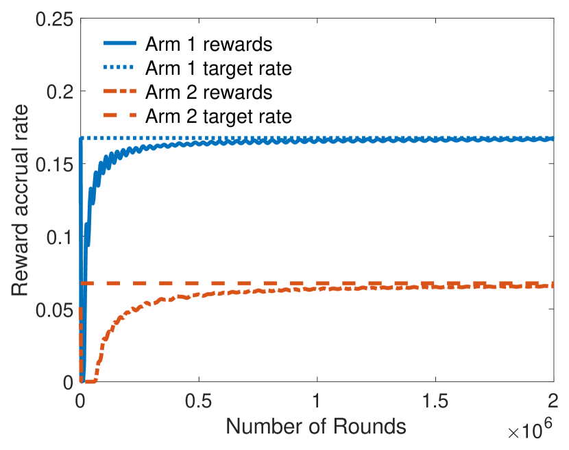
Figure 1: Reward accrual rates in the full-information setting

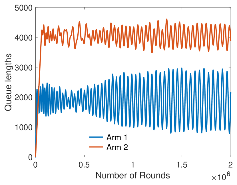
Figure 2: Queue lengths under in the full-information setting

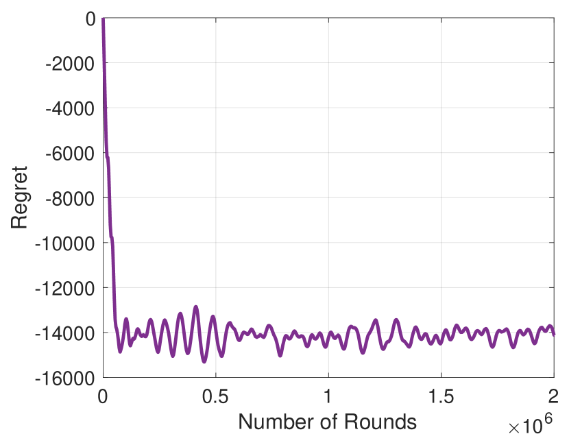
Figure 3: Regret of BanditQ in the full-information setting

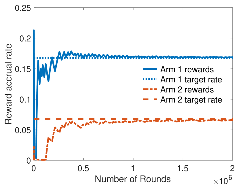
Figure 4: Reward accrual rates in the bandit feedback

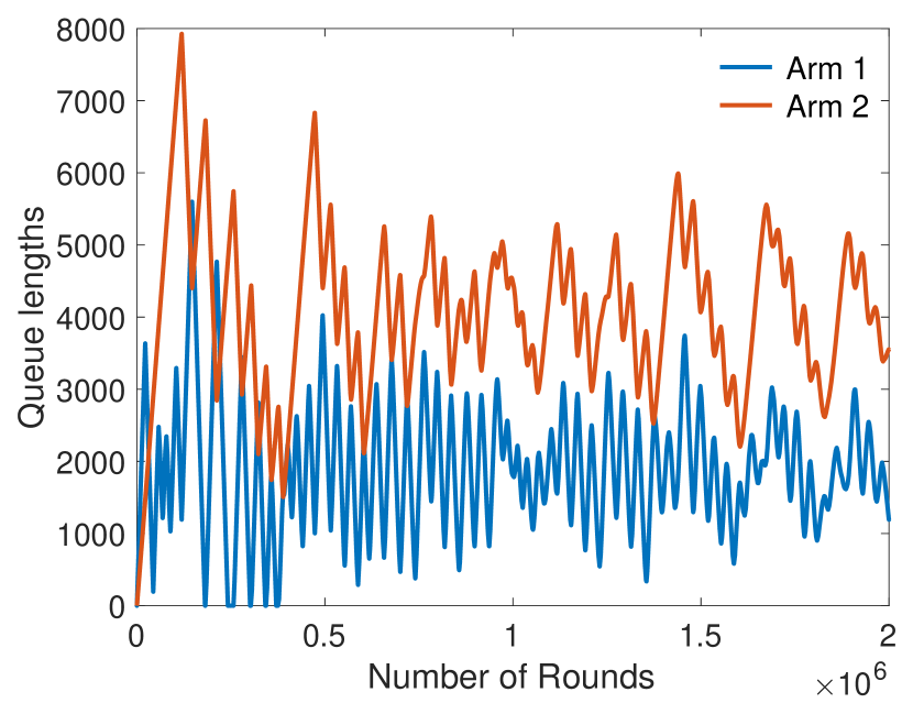
Figure 5: Queue lengths in bandit feedback setting

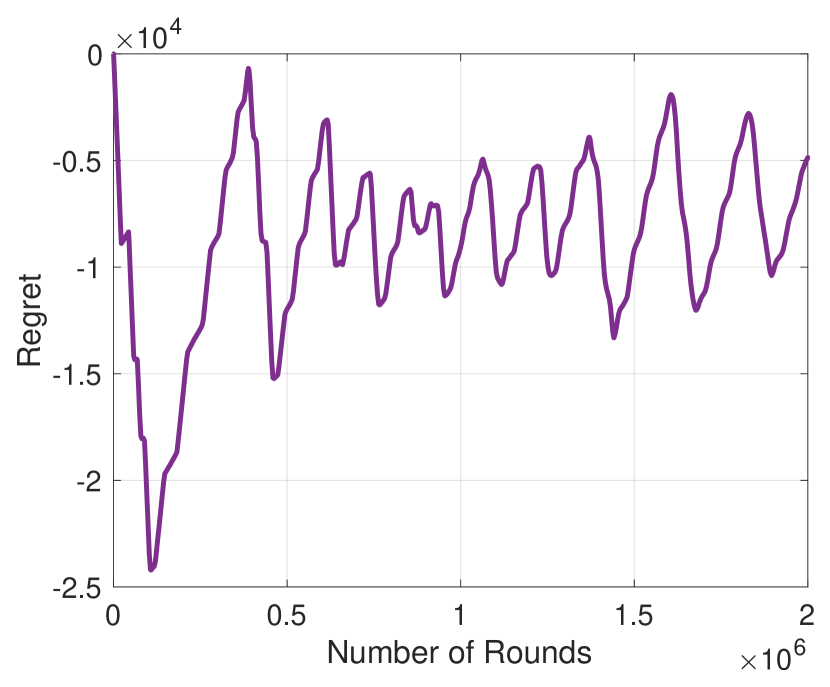
Figure 6: Regret of BanditQ in the bandit feedback setting

6 Conclusion and Open Problems

Since we use adversarial MAB policies as subroutines, it is reasonable to conjecture that the proposed BanditQ policy is robust and would work for adversarial rewards as well. However, proving this statement, or designing fair learning policies in the adversarial setting, are beyond our scope. Improving the regret and the queue length bounds and coming up with instance-dependent logarithmic regret bounds for the fair learning problem would be interesting. Finally, designing an anytime version of the policy that does not need to know the horizon length $T$ in advance would be practically useful.

7 Appendix

7.1 The Feasibility Assumption

Throughout the paper, we assume that the target rate vector $\bm{\vec{\lambda}}$ is feasible. In practice, we can ensure the feasibility by estimating the expected rewards from past data and requiring that condition (2) is strictly satisfied with a reasonable margin. To put it quantitatively, let $\hat{\bm{\mu}}$ be the estimated expected reward vector where it is known that $||\hat{\bm{\mu}}-\bm{\mu}||_{\infty}\leq\epsilon,$ for a small error bound $\epsilon\geq 0$. Then, for the required reward rate vector $\bm{\vec{\lambda}}$ to be feasible, using the first-order Taylor’s series expansion, it is sufficient that:

$$\sum_{i}\frac{\lambda_{i}}{\hat{\mu_{i}}}+\epsilon\sum_{i}\frac{\lambda_{i}}{\hat{\mu_{i}}^{2}}\leq 1.$$ (23)

Although the estimated mean rewards can reasonably be used for determining the feasibility of the required reward rates, they cannot possibly be used for the online selection of the arms with no regret, as even a small constant error in the estimated rewards may lead to a linear regret.

7.2 Proof of Proposition 2

Upon expanding (6), we obtain the following well-known representation of the Lindley recursion [ross1995stochastic]:

$$Q_{i}(t)=\sup_{1\leq\tau\leq t}(0,\lambda_{i}\tau-\sum_{z=t-\tau+1}^{t}r_{i}(z)x_{i}(z)),~{}\forall i\in\mathcal{P}.$$ (24)

Using Proposition 1, we have that $\mathbb{E}Q_{i}(t)\stackrel{{\scriptstyle\textrm{(Jensen's ineq.)}}}{{\leq}}\sqrt{\mathbb{E}Q_{i}^{2}(t)}=O(N^{1/4}T^{3/4}),~{}\forall i\in\mathcal{P},t\in[T].$

Substituting the above bound in Eq. (24), we have for any $i\in\mathcal{P}:$

$$\inf_{1\leq t\leq T}\mathbb{E}\inf_{1\leq\tau\leq t}\big{(}\tau^{-1}\sum_{z=t-\tau+1}^{t}r_{i}(z)x_{i}(z)\big{)}\geq\lambda_{i}-O(\frac{N^{1/4}T^{3/4}}{\tau}),$$

which gives a finite-time guarantee for the expected reward accrual rate for each arm in the protected set $\mathcal{P}.$ Hence, as long as $T^{3/4}/|\mathcal{I}|\to 0,$ we have

$$\liminf_{|\mathcal{I}|\to\infty}|\mathcal{I}|^{-1}\mathbb{E}\big{[}\sum_{t\in\mathcal{I}}r_{i}(t)x_{i}(t)\big{]}\geq\lambda_{i},~{}\forall i\in\mathcal{P}.$$

Finally, using Eq. (24) once again, we can bound the violation penalty as

$$\mathbb{V}(T)\leq\max_{i\in\mathcal{P}}\mathbb{E}Q_{i}(T)=O(N^{1/4}T^{3/4}).$$

7.3 Proof of Proposition 3

Substituting the queue length bounds from Proposition (1) into the inequality (14) and using the fact that $Q_{i}^{2}(T)\geq 0,\forall i,t,$ we have

$$2V\textrm{Regret}_{T}\leq 2T+O(\sqrt{N\sqrt{N}\sum_{\tau=1}^{t}T^{3/2}})+O(T)=O(N^{3/4}T^{5/4}).$$

Since $V=\Theta(\sqrt{T}),$ the above inequality immediately yields $\textrm{Regret}_{T}=O((NT)^{3/4}).$

7.4 Proof of Proposition 4

Define $S_{t}^{2}\equiv\sum_{i}\mathbb{E}Q_{i}^{2}(t).$ From Eq. (13), we have for all $t\in[T]:$

$$S_{t}^{2}+2V\textrm{Regret}_{t}(\bm{x}^{*})\leq 2t+4\sqrt{2\sum_{\tau=1}^{t}S_{\tau}^{2}}+4V\sqrt{2Nt}\leq 2T+4\sqrt{2\sum_{\tau=1}^{T}S_{\tau}^{2}}+4V\sqrt{2NT}.$$

Summing up the above inequality from $t=1$ to $t=T$ and defining $z_{T}\equiv\sqrt{\sum_{\tau=1}^{T}S_{\tau}^{2}},$ the above inequality yields

$$z_{T}^{2}-4Tz_{T}+2V\sum_{t=1}^{T}\textrm{Regret}_{t}(\bm{x}^{*})\leq 2T^{2}+4V\sqrt{2N}T^{3/2}.$$ (25)

Upon completing the square, we have $z_{T}^{2}-4Tz_{T}=(z_{T}-2T)^{2}-4T^{2}\geq-4T^{2}.$ Hence, from (25), we conclude that:

$$\frac{1}{T}\sum_{t=1}^{T}\textrm{Regret}_{t}(\bm{x}^{*})\leq 3\frac{T}{V}+2\sqrt{2NT}.$$

The result follows upon setting $V=\Theta(\sqrt{T}).$

7.5 Proof of Proposition 5

From Eq. (14), we have:

$$\mathbb{E}Q_{i}^{2}(t)\leq 2t+4\sqrt{2\sum_{\tau=1}^{t}\sum_{i}\mathbb{E}Q_{i}^{2}(\tau)}~{}~{}\forall t\geq 1,\forall i.$$ (26)

Since $\lambda_{i}\leq 1,\forall i\in\mathcal{P},$ trivially we have that $Q_{i}(\tau)\leq\tau,\forall\tau,$ i.e., $\mathbb{E}Q_{i}^{2}(\tau)\leq\tau^{2},\forall i,\tau.$ We now use a repeated refinement technique to go from this trivial bound to the claimed bound.

As the induction step, assume that $\mathbb{E}Q^{2}_{i}(\tau)\leq c\tau^{\delta},\forall\tau$ for some $\delta\geq 1$ and $c=64N.$ Then, from Eq. (26), we have that for any $t\geq 1:$

$$\mathbb{E}Q_{i}^{2}(t)\leq 2t+4\sqrt{2Nc\frac{t^{1+\delta}}{1+\delta}}\leq 2t+4\sqrt{Nc}t^{\frac{1+\delta}{2}}\leq ct^{\frac{1+\delta}{2}},~{}\forall i,t,$$

where we have used the fact that $\delta\geq 1$ and $c=64N.$ Hence, the successive upper bounds to the square of the expected queue lengths constitute a sequence of the form $\mathbb{E}Q^{2}_{i}(t)\leq ct^{\delta_{n}},\forall i,t,$ where $\delta_{n+1}=\max(1,\frac{1+\delta_{n}}{2}),$ with $\delta_{1}=1.$ It is easy to verify that the above sequence $\{\delta_{n}\}_{n\geq 1}$ converges to $1.$ Hence, we have that $\mathbb{E}Q_{i}^{2}(t)\leq 64Nt.$ Finally, using Jensen’s inequality, we conclude that $\mathbb{E}Q_{i}(t)\leq\sqrt{\mathbb{E}Q_{i}^{2}(t)}\leq\sqrt{ct}\leq 8\sqrt{Nt}.$ This completes the proof of the result.

7.6 Bound on the diameter of the queueing processes $\{\textbf{Q}(t)\}_{t=1}^{T}$

Proposition 7.

Upon setting $V_{t}=V=\Theta(\sqrt{T}),t\in[T],$ under the action of the BanditQ policy, we have the following bound on the maximum diameter of the queueing processes

$$\mathbb{E}\big{[}\max_{i,t\in[T]}Q_{i}(t)\big{]}=\tilde{O}(N^{1/4}T^{3/4}).$$

Proof.

Working similar to Eq. (13), we have the following sample-path wise bound on the queue lengths:

$$\sum_{i}Q_{i}^{2}(t) \leq 2(V+1)t+2\sum_{\tau=1}^{t}\sum_{i}Q_{i}(\tau-1)\big{(}\lambda_{i}-r_{i}(\tau)x_{i}^{*}\big{)}+2\textrm{Regret}^{\Xi}_{t}$$ (27)

$$\stackrel{{\scriptstyle(a)}}{{\leq}} 2(V+1)T+\tilde{O}(\sqrt{N\sum_{\tau=1}^{T}\sum_{i}Q_{i}^{2}(\tau)}+NV\sqrt{T}+\sqrt{N}T^{3/2})+2\sum_{i}M_{t}^{i},$$

where, in (a), we have substituted an upper-bound to the regret from Eq. (16) and for each $i\in[N],$ defined the processes

$$M_{t}^{i}=\sum_{\tau=1}^{t}Q_{i}(\tau-1)\big{(}\lambda_{i}^{\prime}-r_{i}(\tau)x_{i}^{*}\big{)},~{}t\geq 1.$$ (28)

where $\lambda_{i}^{\prime}\stackrel{{\scriptstyle(\textrm{def.})}}{{=}}x_{i}^{*}\mathbb{E}r_{i}(\tau)=x_{i}^{*}\mu_{i}\geq\lambda_{i}.$ Hence, recalling that $V=\Theta(\sqrt{T}),$ we have

$$\max_{i,t\in[T]}Q_{i}^{2}(t)\leq\tilde{O}(\sqrt{N\sum_{\tau=1}^{T}\sum_{i}Q_{i}^{2}(\tau)}+\sqrt{N}T^{3/2})+2\sum_{i}\max_{t}M_{t}^{i}.$$

Taking expectation of both sides, we have

$$\mathbb{E}\big{[}\max_{i,t\in[T]}Q_{i}^{2}(t)\big{]} \leq \tilde{O}(\sqrt{N\sum_{\tau=1}^{T}\sum_{i}\mathbb{E}Q_{i}^{2}(\tau)}+\sqrt{N}T^{3/2})+2\sum_{i}\mathbb{E}\big{[}\max_{t\in[T]}M_{t}^{i}\big{]}$$ (29)

$$\leq \tilde{O}(\sqrt{N}T^{3/2})+2\sum_{i}\mathbb{E}\big{[}\max_{t}M_{t}^{i}\big{]},$$

where in the last step, we have used the bound from (22). Next, we claim that each of the processes $\{M_{t}^{i}\}_{t\geq 1}$ is a zero-mean Martingale process with respect to the natural filtration $\{\mathcal{F}_{\tau}\}_{\tau\geq 1}$. This follows from the definition (28) as $Q_{i}(\tau-1)\in\mathcal{F}_{\tau-1}$ is pre-visible and the random variable $r_{i}(\tau)$ is independent of $\mathcal{F}_{\tau-1}$ s.t. $\mathbb{E}(\lambda_{i}^{\prime}-r_{i}(\tau)x_{i}^{*})=0.$ Using classic results [doob1953stochastic, Theorem 3.4], [dubins1988sharp], we know that the diameter of a Martingale with a last term is bounded by twice the square root of the variance of the last term. Hence,

$$\mathbb{E}[\max_{t\in[T]}M^{i}_{t}]=O(\sqrt{\mathbb{E}(M^{i}_{T})^{2}}).$$

Now we have

$$\mathbb{E}(M_{T}^{i})^{2}\leq\sum_{\tau=1}^{T}\mathbb{E}Q_{i}(\tau-1)^{2}\leq\sqrt{N}T^{5/2},$$

where in the last step, we have used (22). Combining the above with Eq. (29), we obtain the desired bound for the diameter of the queueing process:

$$\mathbb{E}\big{[}\max_{i,t\in[T]}Q_{i}^{2}(t)\big{]}\leq\tilde{O}(\sqrt{N}T^{3/2})+O(N^{1/4}T^{5/4})=\tilde{O}(\sqrt{N}T^{3/2}).$$

The result stated in the lemma finally follows from an application of the Jensen’s inequality. ∎

7.7 Proof of Theorem 3

From Eq. (19), we have that

$$2V\textrm{Regret}_{T} \leq 2T+\tilde{O}(\sqrt{N\sum_{\tau=1}^{T}\sum_{i}\mathbb{E}Q_{i}^{2}(\tau)}+NV\sqrt{T}+V\sqrt{NT}+\sqrt{NT}\mathbb{E}\big{[}\max_{i,t\in[T]}(Q_{i}(t))\big{]}$$

$$\leq \tilde{O}(N^{5/4}T^{5/4}+NV\sqrt{T}+N^{3/4}T^{5/4}).$$

where we have substituted the bounds from Eq. (22) and Proposition 7. Finally, dividing both sides by $V=\Theta(\sqrt{T}),$ we have

$$\textrm{Regret}_{T}=\tilde{O}(N^{5/4}T^{3/4}).$$

7.8 Pseudocode for the BanditQ policy in the Bandit-Information set up

As discussed in the main text, the BanditQ policy in the Bandit feedback setting uses the scale-free MAB algorithm of putta2022scale in conjunction with the surrogate reward function defined in Eq. (18). The complete pseudocode of the BanditQ policy is given below in Algorithm 2.

Algorithm 2 BanditQ Policy in the Bandit-feedback setting

1:Input: Target reward rate vector $\bm{\vec{\lambda}}$, $\eta\leftarrow N,\gamma\leftarrow 1/2$, Regularizer $F(q)=\sum_{i=1}^{N}(f(q(i)-f(1/N)),$ where $f(x)=-\log(x).$

2:$\bm{Q}\leftarrow\bm{0},\bm{p}\leftarrow[1/N,1/N,\ldots,1/N],V\leftarrow\sqrt{T},S\leftarrow 1,\bm{\tilde{R}}\leftarrow 0.$ $\triangleright$ Initialization

3:for each round $t=1:T$: do

4:     $\bm{x}\leftarrow(1-\gamma)\bm{p}+\gamma/N$. $\triangleright$ Updating the sampling distribution

5:     Sample an arm $I_{t}\in[N]$ from the distribution $\bm{x}$.

6:     Observe the reward of the selected arm $r_{I_{t}}(t)$$\triangleright$ Bandit feedback

7:     $Q_{i}=\big{(}Q_{i}+\lambda_{i}-r_{i}(t)\mathds{1}(I_{t}=i)\big{)}^{+},~{}\forall i\in\mathcal{P}.$$\triangleright$ Updating the queues

8:     $r^{\prime}_{i}\leftarrow\big{(}Q_{i}+V\big{)}r_{i}(t)\mathds{1}(I_{t}=i),~{}\forall i$ $\triangleright$ Computing the surrogate rewards

9:     $\tilde{r}_{i}\leftarrow\frac{r^{\prime}_{i}}{x_{i}}\mathds{1}(I_{t}=i)$ $\triangleright$ Estimating the rewards via the inverse propensity scores (IPS)

10:     $\bm{\tilde{R}}\leftarrow\bm{\tilde{R}}+\bm{\tilde{r}}$ $\triangleright$ Updating the cumulative estimated surrogate rewards

11:     $\gamma\leftarrow\min(1/2,\sqrt{N/t}).$

12:     $S\leftarrow S+\eta^{-1}\sup_{q\in\Delta_{N}}(\langle\tilde{\bm{r}},\bm{q}-\bm{p}\rangle-\textrm{Breg}_{F}(\bm{q}||\bm{p}).$

13:     $\eta\leftarrow N/S$ $\triangleright$ Adaptively choosing the learning rate

14:     $\bm{p}\leftarrow\arg\min_{\bm{q}\in\Delta_{N}}\big{[}F(\bm{q})-\eta\langle\bm{q},\bm{\tilde{R}}\rangle\big{]}$ $\triangleright$ The FTRL step

15:end for each

In line 12 of the pseudocode, $\textrm{Breg}_{F}(x||y)$ denotes the usual Bregman divergence between the points $x$ and $y$ with respect to the convex function $F(\cdot),$ i.e.,

$$\textrm{Breg}_{F}(x||y)=F(x)-F(y)-\langle\nabla F(y),x-y\rangle.$$

7.9 Efficient Implementation of the Optimization Module

To speed up the simulation, we implemented a custom-made optimizer for the optimization steps 12 and 14 involved in the BanditQ algorithm in the bandit-feedback setting. For this, we directly solved the KKT optimality condition, where we computed the optimal KKT multiplier by using the classic Newton-Raphson root-finding algorithm. This empirically resulted in about two orders of magnitude speed-up compared to using standard convex optimization packages such as CVX [grant2011cvx].

Let $\bm{r}\in\mathbb{R}^{N}$ be a given $N$-dimensional real vector. After some simple algebraic manipulations, both the optimization problems in steps 12 and 14 of Algorithm 2 can be expressed in the following form:

$$\texttt{OPT}(\bm{r}):~{}\max\sum_{i=1}^{N}\log x_{i}+\langle\bm{r},\bm{x}\rangle$$ (30)

Subject to,

$$\sum_{i}x_{i}=1,~{}x_{i}\geq 0,~{}\forall i\in[N].$$ (31)

Since the objective function (30) is strictly concave, and the constraint (31) is linear, using the KKT condition, a probability vector $\bm{x}^{*}$ is an optimal point for the above problem if and only if there exists a real number $\mu\in\mathbb{R}$ s.t.

$$\frac{1}{x_{i}^{*}}+r_{i}+\mu=0\implies x_{i}^{*}=-(r_{i}+\mu)^{-1},~{}\forall i,$$ (32)

where $\bm{x}^{*}$ satisfies the feasibility condition (31). For the non-negativity constraint on $\bm{x}^{*}$, we must have:

$$r_{i}+\mu<0\implies\mu<-\max_{i}r_{i}.$$

Finally, we require that

$$\sum_{i}x_{i}^{*}=1.$$

i.e.,

$$\sum_{i}\frac{1}{r_{i}+\mu}-1=0.$$ (33)

We now use the Newton-Raphson method for solving (33) starting from $\mu^{(0)}=-\max_{i}r_{i}-1.$ The algorithm is given below:

Algorithm 3 Custom optimizer for the problem OPT ($\bm{r}$)

1:Input: $\bm{r},$ $\texttt{tolerance}\leftarrow 10^{-8}.$

2:$\mu\leftarrow-\max_{i}r_{i}-1,\texttt{error}\leftarrow 1.$

3:while $\texttt{error}>\texttt{tolerance}$ do

$$\mu\leftarrow\mu+\frac{\sum_{i}\frac{1}{r_{i}+\mu}-1}{\sum_{i}\frac{1}{(r_{i}+\mu)^{2}}}.$$

$\texttt{error}\leftarrow|\sum_{i}\frac{1}{r_{i}+\mu}-1|.$

4:end while

5:$x_{i}^{*}\leftarrow-(r_{i}+\mu)^{-1},~{}\forall i.$

6:Return $\bm{x}^{*}.$

7.10 Additional Numerical Results: Comparison with an Oracle Policy

In this section, we compare the performance of the BanditQ policy with an Oracle policy that knows the optimal fraction of pulls of each arm to satisfy the required reward rate constraints. With the given mean reward $\bm{\mu}$ and the required reward rate vector $\bm{\lambda}$, the optimal fraction of pulls can be easily computed to be $f_{1}=\nicefrac{{\lambda_{1}}}{{\mu_{1}}}=\nicefrac{{1}}{{2}},f_{2}=\nicefrac{{\lambda_{2}}}{{\mu_{2}}}=\nicefrac{{1}}{{3}},f_{3}=0,f_{4}=1-(\nicefrac{{1}}{{2}}+\nicefrac{{1}}{{3}})=\nicefrac{{1}}{{6}},f_{5}=0.$ In the above computation, we have used the fact that Arm #4 is the most-rewarding arm. We emphasize that the oracle policy should have exact knowledge of the mean reward vector $\bm{\mu}$ - a non-zero error in the value of the reward vector either lead to not achieving the target rates or having a linear regret or both.

Note that the online policy proposed by patil2021achieving cannot be used with the above profile of fraction of pulls as their policy requires the required fraction of each arm to be at most $1/N-1=\nicefrac{{1}}{{4}}.$ Hence, we use the UCB-based policy proposed by li2019combinatorial, called Learning with Fairness Guarantee (LFG), as the benchmark. LFG uses queue variables to balance meeting the target fraction of pulls and achieving the small regret. However, as stated in li2019combinatorial, the best-known regret bound of the LFG policy increases linearly with time.

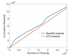
Figure 7: Comparison of reward accrued by the BanditQ policy and the Oracle LFG policy ($\eta=100$)

Observation:

From Figure 7, we see that the proposed BanditQ policy yields strictly better cumulative rewards compared to the oracle LFG policy that knows the optimal fraction of arm pulls to meet the given reward rate constraints. This result can be attributed to the fact that the BanditQ policy directly takes into account the reward realizations through the queue evolutions, whereas the Oracle LFG policy works based on the expected rewards only.

References

- Sweeney (2013) Latanya Sweeney. Discrimination in online ad delivery. Communications of the ACM, 56(5):44–54, 2013.
- Hao (2019) Karen Hao. Facebook’s ad-serving algorithm discriminates by gender and race. MIT Technology Review, 2019.
- Cesa-Bianchi and Lugosi (2006) Nicolo Cesa-Bianchi and Gábor Lugosi. Prediction, learning, and games. Cambridge university press, 2006.
- Bubeck et al. (2012) Sébastien Bubeck, Nicolo Cesa-Bianchi, et al. Regret analysis of stochastic and nonstochastic multi-armed bandit problems. Foundations and Trends® in Machine Learning, 5(1):1–122, 2012.
- Lattimore and Szepesvári (2020) Tor Lattimore and Csaba Szepesvári. Bandit algorithms. Cambridge University Press, 2020.
- Joseph et al. (2016) Matthew Joseph, Michael Kearns, Jamie H Morgenstern, and Aaron Roth. Fairness in learning: Classic and contextual bandits. Advances in neural information processing systems, 29, 2016.
- Gillen et al. (2018) Stephen Gillen, Christopher Jung, Michael Kearns, and Aaron Roth. Online learning with an unknown fairness metric. Advances in neural information processing systems, 31, 2018.
- Bechavod et al. (2020) Yahav Bechavod, Christopher Jung, and Steven Z Wu. Metric-free individual fairness in online learning. Advances in neural information processing systems, 33:11214–11225, 2020.
- Hossain et al. (2021) Safwan Hossain, Evi Micha, and Nisarg Shah. Fair algorithms for multi-agent multi-armed bandits. Advances in Neural Information Processing Systems, 34:24005–24017, 2021.
- Huang et al. (2022) Wen Huang, Lu Zhang, and Xintao Wu. Achieving counterfactual fairness for causal bandit. In Proceedings of the AAAI Conference on Artificial Intelligence, volume 36, pages 6952–6959, 2022.
- Patil et al. (2021) Vishakha Patil, Ganesh Ghalme, Vineet Nair, and Yadati Narahari. Achieving fairness in the stochastic multi-armed bandit problem. The Journal of Machine Learning Research, 22(1):7885–7915, 2021.
- Claure et al. (2020) Houston Claure, Yifang Chen, Jignesh Modi, Malte Jung, and Stefanos Nikolaidis. Multi-armed bandits with fairness constraints for distributing resources to human teammates. In Proceedings of the 2020 ACM/IEEE International Conference on Human-Robot Interaction, pages 299–308, 2020.
- Li et al. (2019) Fengjiao Li, Jia Liu, and Bo Ji. Combinatorial sleeping bandits with fairness constraints. IEEE Transactions on Network Science and Engineering, 7(3):1799–1813, 2019.
- Celis et al. (2019) L Elisa Celis, Sayash Kapoor, Farnood Salehi, and Nisheeth Vishnoi. Controlling polarization in personalization: An algorithmic framework. In Proceedings of the conference on fairness, accountability, and transparency, pages 160–169, 2019.
- Chen et al. (2020) Yifang Chen, Alex Cuellar, Haipeng Luo, Jignesh Modi, Heramb Nemlekar, and Stefanos Nikolaidis. Fair contextual multi-armed bandits: Theory and experiments. In Conference on Uncertainty in Artificial Intelligence, pages 181–190. PMLR, 2020.
- Cai et al. (2018) Kechao Cai, Xutong Liu, Yu-Zhen Janice Chen, and John CS Lui. An online learning approach to network application optimization with guarantee. In IEEE INFOCOM 2018-IEEE Conference on Computer Communications, pages 2006–2014. IEEE, 2018.
- Badanidiyuru et al. (2018) Ashwinkumar Badanidiyuru, Robert Kleinberg, and Aleksandrs Slivkins. Bandits with knapsacks. Journal of the ACM (JACM), 65(3):1–55, 2018.
- Immorlica et al. (2022) Nicole Immorlica, Karthik Sankararaman, Robert Schapire, and Aleksandrs Slivkins. Adversarial bandits with knapsacks. Journal of the ACM, 69(6):1–47, 2022.
- Xia et al. (2015) Yingce Xia, Haifang Li, Tao Qin, Nenghai Yu, and Tie-Yan Liu. Thompson sampling for budgeted multi-armed bandits. In Proceedings of the 24th International Conference on Artificial Intelligence, IJCAI’15, page 3960–3966. AAAI Press, 2015. ISBN 9781577357384.
- Orabona (2019) Francesco Orabona. A modern introduction to online learning. arXiv preprint arXiv:1912.13213, 2019.
- Neely (2010) Michael J Neely. Stochastic network optimization with application to communication and queueing systems. Synthesis Lectures on Communication Networks, 3(1):1–211, 2010.
- Lindley (1952) David V Lindley. The theory of queues with a single server. In Mathematical Proceedings of the Cambridge Philosophical Society, volume 48, pages 277–289. Cambridge University Press, 1952.
- Huang et al. (2023) Jiatai Huang, Leana Golubchik, and Longbo Huang. Queue scheduling with adversarial bandit learning. arXiv preprint arXiv:2303.01745, 2023.
- Koolen and Van Erven (2015) Wouter M Koolen and Tim Van Erven. Second-order quantile methods for experts and combinatorial games. In Conference on Learning Theory, pages 1155–1175. PMLR, 2015.
- Wang and Carreira-Perpinán (2013) Weiran Wang and Miguel A Carreira-Perpinán. Projection onto the probability simplex: An efficient algorithm with a simple proof, and an application. arXiv preprint arXiv:1309.1541, 2013.
- Putta and Agrawal (2022) Sudeep Raja Putta and Shipra Agrawal. Scale-free adversarial multi armed bandits. In International Conference on Algorithmic Learning Theory, pages 910–930. PMLR, 2022.
- Hadiji and Stoltz (2023) Hédi Hadiji and Gilles Stoltz. Adaptation to the range in k–armed bandits. Journal of Machine Learning Research, 24(13):1–33, 2023.
- Ross (1995) Sheldon M Ross. Stochastic processes. John Wiley & Sons, 1995.
- Doob (1953) Joseph L Doob. Stochastic processes. John Wiley & Sons, 1953.
- Dubins and Schwarz (1988) Lester E Dubins and Gideon Schwarz. A sharp inequality for sub-martingales and stopping-times. Astérisque, 157(158):129–145, 1988.
- Grant et al. (2011) Michael Grant, Stephen Boyd, and Yinyu Ye. Cvx: Matlab software for disciplined convex programming, 2011.