Individualized conformal

Abstract

The problem of individualized prediction can be addressed using variants of conformal prediction, obtaining the intervals to which the actual values of the variables of interest belong. Here we present a method based on detecting the observations that may be relevant for a given question and then using simulated controls to yield the intervals for the predicted values. This method is shown to be adaptive and able to detect the presence of latent relevant variables.
Keywords: Conformal Prediction, Individualized Inference, Split and Jacknife Distribution-Free Inference.

1 Introduction

We present a novel approach to individualized conformal prediction, intended to yield the intervals in which the actual predicted values of certain variables might be found. We proceed by first detecting relevant observations for a given target query using a technique reminiscent to divide and conquer (Chen et al., (2021)). Then we apply a data augmentation procedure similar to the generation of repro samples (Xie and Wang, (2022)), simulating controls as if they were bootstrapped (as in Tran et al., (2017)). The development of this approach is based on the statistical technique known as Conformal Prediction.

Conformal Prediction (CP) is a distribution-free prediction methodology usually based on machine learning systems. CP generates predictions about new test data points on the basis of training labeled datasets, only assuming the exchangeability of the data. It requires a pre-specified level that restricts the frequency of errors that the algorithm is allowed to make (see, for instance, Vovk et al., (2022), Xie and Zheng, (2022), Lei et al., (2018), Barber et al., (2021)). Variants of this methodology are split and jacknife distribution-free conformal inference (Lei et al., (2018)). A recent development that is closely related to our contribution is the adaptive version of CP, based on the application of self-supervised learning (Seedat et al., (2023)).

Another strand in the literature that is relevant for our approach is individualized inference. This is a particularly useful methodology in the case of large datasets, since it addresses the heterogeneity of data. One approach is based on generating iGroups of data sharing common features with targeted individuals (Cai et al., (2021)). Alternatively, in the iFusion approach the group of relevant data is generated by fusing the inferences from individuals that are similar to the targeted one (Shen et al., (2020)). Individualized inference is also invoked to categorize cases by mixing Gaussian processes generated by individuals with related features (Alaa and Van Der Schaar, (2017)).

The specific techniques used to carry out the inferences are varied. Chernozhukov et al., (2017) develops a Debiased Machine Learning method to obtain inferences about specific parameters. More traditional methods can also be applied, like inferring confidence (Xie and Singh, (2013), Schweder and Hjort, (2016)) and predictive (Shen et al., (2018)) distributions, which could be seen as “Bayesian-like frequentist techniques” that derive distributions up from observed data. In practical terms, an important contribution is the implementation in the R language of trainable $p$-value functions (instead of just $p$-values) by Infanger and Schmidt-Trucksäss, (2019).

Our own approach has the following features:

• It is adaptive.

• It admits new unlabeled data as input.

• It satisfies the condition of exchangeability by restricting the focus on relevant, and then simulated, data.

• It detects empirically the presence of latent relevant variables, by implicitly getting rid of the factor that generates a failure of the i.i.d. condition.

This paper is structured as follows. We first present, in Section 2, the motivation of our proposal. Section 3 details a procedure implementing the method developed. Section 4 presents the empirical setting in which we test the methodology and the corresponding results. Section 5 concludes by presenting ideas for further developments.

2 Motivation

We assume, as in Delbianco et al., (2021), a statistical model of a data generation process, which can be described as $\{\mathcal{O},\mathcal{P}\}$, where $\mathcal{O}$ is the set of observations while $\mathcal{P}=\{P_{\theta}:\theta\in\Theta\}$ is a family of probability distributions over $\mathcal{O}$ and $\Theta$ is the space of parameters of the model. The goal is again to estimate intervals for the parameters in response to any query q, where q is a specific request for information under a given inference method $\mathcal{I}$ applied on the database.

The query defines several dimensions. First, $\mathcal{O}$ consists of entries $\{o_{i}=\langle x_{i},y_{i}\rangle\}_{i=1,\ldots,n}$, where $x_{i}$ is a matrix of $p$ variables and $n$ observations, the tail of $o_{i}$, while $y_{i}$ is the head, a vector of dimension $n$. The query $q$ consists of a tail, $x_{0}$, with no head, and with $x_{o}\neq x_{i}$, for $i=1,\ldots,n$. We assume that there exists a class of latent variables $\mathcal{S}$ such that given a query $q$ there exists a corresponding $s_{q}\in\mathcal{S}$ yields a class of relevant observations $\mathcal{O}_{q}\subseteq\mathcal{O}$ .

Figure 1: Latent relevant area $S_{q}$

A particular value of a tail $q$, is associated to a latent variable $s_{q}$ that yields the relevant space of tails $x\in X_{q}$ and as a consequence allows to infer the corresponding class of heads $y\in Y_{q}$. Then, this bi-dimensional figure can be extended to a tri-dimensional one, with the sequence of different queries as a third axis. This represents how the relevant set varies according to $q$, learning the associated $\theta^{q}$.

We then generate a class of controls $\bar{\mathcal{O}}_{q}$ verifying that $\mathcal{O}_{q}\subseteq\bar{\mathcal{O}}_{q}$. Based on $\bar{\mathcal{O}}_{q}$ the application of the inference procedure $\mathcal{I}$ yields an interval $\mathbf{I}_{q}$, with $\theta^{q}\in\mathbf{I}_{q}$ such that $\bar{\mathcal{O}}_{q}$ can be understood as a set of draws from a distribution $\bar{P}_{\theta^{q}}\in\mathcal{P}$ . The relevant set of observations is given by $\mathcal{O}_{q}=f_{\mathcal{S}}(s_{q})$, where $f_{\mathcal{S}}:\mathcal{S}\rightarrow 2^{\mathcal{O}}$ characterizes a selection procedure.

Figure 2: Simulated controls $\in\bar{\mathcal{O}}_{q}$

The relevant set $\mathcal{O}_{q}$, detected by means of $f_{\mathcal{S}}$, is extended to an enlarged set, $\bar{\mathcal{O}}_{q}$. The difference in the inference based in new controls can be measured as $\Delta_{\theta^{q}}=E(\bar{P}_{\theta^{q}})-E(P_{\theta^{q}})$.

For an example consider the case of different economies $i$, each one described by a vector of a few macroeconomic variables $o_{i}=\langle x_{i},y_{i}\rangle$, where $y_{i}$ is the GDP of country $i$. We can ask, for any given economy $\bar{o}\notin\mathcal{O}$ what is its expected GDP in five years, knowing only $\bar{x}$. Now assume that a latent variable is the productivity of the leading sectors in an economy. Then we can group all the countries in $\mathcal{O}$ with a similar productivity as that of $\bar{o}$ and generate a class of controls based on this choice.

Taking another example, we can consider a dataset of programs, students and grades. For a new student, we can ask different questions. For instance, how long will take for a new student to finish her studies? What is the probability of her changing majors? or the probability of dropping out school?, among many other possible queries about this particular student that could be answered with the observations in the dataset. Of course, a different query may require different controls. And this can be true for both the variables and the observations. So the $s_{q}$ latent variable will yield the portion of observations that is relevant given $q$, and will let us estimate $f_{\mathcal{S}}$ in order to simulate new controls and gain robustness in the inference.

To proceed in this way we need to specify, for each $q$ a latent variable (or set of latent variables) that are relevant for the query. Then, we have to distinguish its range using some proxy or measurement on the available $\mathcal{O}$. This will yield the class of relevant observations. For the sake of simplicity, we could assume that exists only two types of query, $q_{A}$ and $q_{B}$, and the latent variable $s_{q}$ defines $\mathcal{O}_{q_{A}}$ and $\mathcal{O}_{q_{B}}$. This setting can be later generalized to cases of more than two types of query. In the particular example of the students, let us assume that there are two types of students, associated to a latent variable (which can capture, for instance, socioeconomic or cognitive advantages). Then, each $q$ will be associated to its corresponding type of student and according to $f_{\mathcal{S}}$, mapped to the class of observations of students of that type.

As said, the class $\mathcal{O}_{q}$ is that of the entries in $\mathcal{O}$ that are relevant to answering $q$. But once obtained these relevant observations, a robust inference requires generating new controls, not present in $\mathcal{O}_{q}$. This is achieved by creating pairs $\langle x,y\rangle$ similar to those in $\mathcal{O}_{q}$ but without assuming that they share with the latter a common value of the latent variable. This means that only the observable features of the entries $o\in\mathcal{O}_{q}$ must be used to create fictitious controls in $\bar{\mathcal{O}}_{q}$, for instance as in the examples of Section 5 of Delbianco et al., (2021).

3 Framework

As said, our procedure takes elements from different approaches:

• Lei et al., (2018) presents three versions of the conformal prediction method. One is based on the original formulation of Vovk et al., (2022). The other two are the split conformal and the jackknife alternatives.

• Lei et al., (2018) also presents an R code for distribution-free prediction, which we modify to be applied in our project.

• We use both a classical linear procedure and one based on elastic nets. Alternatively, we can include a Gaussian Kernel regression to implement a non-parametric approach. Other methods can be also easily applied using the estimations and predictions generated by the R package Caret (Kuhn, (2008)), which is convenient for the following additional reasons:

  1. It implements a previous training stage, cross-validating the results in order to choose the meaningful features. It even allows to apply methodologies that split the entries of the training database in a different way as conformal prediction. This allows to make a finer selection of the $n_{r}$ relevant entries and the $2n_{r}$ controls.

  2. It allows to choose from almost fifty prediction methodologies, among which are GLM, Kernel, Quantile regression, Random Forest, etc. But, as said, we use in a first run only regression and LASSO.

• The parameters in our exercise are: $\alpha$ for confidence intervals, $\rho$ for splitting in split conformal prediction, and $\gamma$ for cosine similarity (for percentile similarity we also use $\alpha$).

• We add two stages of prediction, using the concept of relevance for individual inference of our original presentation (Delbianco et al., (2021)):

  1. The first stage evaluates the relevance of entries in the database for each new observation, based on the degree of similarity with the rest of the database. The relevance is defined, when $p$ is small, in terms of the percentage of distance between the tails of observations and those in the database. Otherwise, when the dimension of the tails is large (in particular when $p>n$), we apply a cosine-based measure. That is, the closer to 1 the cosine between the respective tails is, the more relevant is an entry for a new observation. A prediction can be made on the basis of the relevant entries: a possible value of the head of the new observation can be predicted, using a standard prediction method on the subset of relevant entries of the original database.

  2. A second type of prediction is based on the generation of controls using the relevant entries collected in the previous stage. For each individual entry in a query for $X_{0}$, we generate another tail-head vector by adding a small noise to its features. Thus, given $n_{r}$ relevant entries ($n_{r}<<n$), we obtain $2n_{r}$ control vectors at this stage.

We will now present the pseudocode of the algorithm that yields the intervals of prediction for the queries. Notice that for simplicity we do not state explicitly the steps and parameters of the methods drawn from $\mathcal{M}$ (Lei et al., (2018), implemented in the R package ConformalInference), $\mathcal{A}$ (implemented in the Caret package) and the similarity functions in $\mathcal{S}$.

Algorithm 1 Individualized Conformal Prediction

Input: $X$, $Y$, $X_{0}$, Regression method $\mathcal{A}$, Similarity method $\mathcal{S}$, Conformal method $\mathcal{M}$, miscoverage level $\alpha$, Similarity intensity $\gamma$

Output: Prediction intervals for each element in $X_{0}$

$\alpha\leftarrow\alpha_{i}\in\{0;1\}$

$\gamma\leftarrow\gamma_{i}\in\{0;1\}$

$\mathcal{A}\leftarrow\mathcal{A}_{i}$ $\triangleright$ OLS, LASSO, Kernel

$\mathcal{M}\leftarrow\mathcal{M}_{i}$ $\triangleright$ Conformal, Split, Jackkinfe

$\mathcal{S}\leftarrow\mathcal{S}_{i}$ $\triangleright$ Percentile, Cosine

for each $x\in X_{0}$ do

     1.1 Predict $y_{0}$ with $\mathcal{A}$ and $X$

     1.2 Use residuals and $\mathcal{M}$ $\rightarrow$ interval ($\mathcal{C}$)

     2.1 Use $\gamma$ and $\mathcal{S}$ $\rightarrow$ $X_{rel}$

     2.2 Predict $y_{0}$ with $\mathcal{A}$ and $X_{rel}$

     2.3 Use residuals and $\mathcal{M}$ $\rightarrow$ relevant interval ($\mathcal{C}_{rel}$)

     3.1 Simulate $X_{sim}$ mimicking the distribution of $X_{rel}$ and $n{sim}=n{rel}$

     3.2 Predict $y_{0}$ with $\mathcal{A}$ and $X_{sim}$

     3.3 Use residuals and $\mathcal{M}$ $\rightarrow$ relevant and simulated interval ($\mathcal{C}_{sim}$)

end for each $x\in X_{0}$

Return: $\mathcal{C}$, $\mathcal{C}_{rel}$, $\mathcal{C}_{sim}$

A diagrammatic representation of this algorithm is depicted in Figure 3. We can see that there are three paths, leading either to $\mathcal{C}$, $\mathcal{C}_{rel}$ or $\mathcal{C}_{sim}$. Each of those can be executed independently, although the latter two share a stage of detection of relevant observations.

In Figure 3 the main decisions to be made are represented by the red circle. Each single change in the choices made can lead to different results. In principle we do not know how robust are the results to small differences in the choices made, but some are easily predicted. So, for instance, a lower significance level $\alpha$ yields longer intervals while a higher similarity level $\gamma$ reduces the number of relevant observations. Other than that, the actual choices of estimation method, type of conformal inference and relevance criterion depend on the problems at hand and how the user assesses them.

Figure 3: Diagram of Algorithm 1.

The red circle encloses the initialization stage of the algorithm in which the estimation method, the type of conformal inference and the relevance criterion are chosen. These decisions impact on all the outputs. Up from this point, three alternative paths can be taken. The first one does not involve relevant data and yields the standard result of conformal prediction, $\mathcal{C}$. The second and the third paths require selecting a subset of observations of $D$ that are similar to the query $x_{0}$. From then on, two possible alternatives consist in either using just that subset to obtain the confidence interval $\mathcal{C}_{rel}$ or to generate a synthetic sample enlarging the class of relevant data to obtain $\mathcal{C}_{sim}$. In Algorithm 1 these alternative paths are denoted 1, 2 and 3, with their respective steps (1.1, 1.2, 2.1, etc.)

To compare the results of the different methods chosen we apply four metrics. Two of them, $A$ and $B$, do not evaluate the intervals but the predicted values of the variable of interest.

• Distance from the forecast: the absolute value of the difference between the true value $y_{0}$ and the value predicted by $\mathcal{A}$ on $X$, $X_{rel}$, or $X_{sim}$. Naturally, the smaller $A$ the more accurate the prediction.

• Distance from the forecast, as a percentage of $y_{0}$: it is defined as $\frac{A}{y_{0}}$ indicating how far is the forecast from the actual one in proportion to the latter. In this case it is not clear that smaller is always better.

• Length of the interval: the difference between the upper and lower limits of the intervals generated by Algorithm 1. The length of an interval depends on $\alpha$, but at the same significance level, a shorter interval indicates a lower uncertainty about the forecast.

• Normalized distance from the forecast: it is defined as $\frac{A}{C}$. It indicates how large is the error with respect the length of the interval.

Two additional measures may also provide information about the quality of the intervals generated by Algorithm 1, namely coverage and excess (see Seedat et al., (2023)). In the exercises reported in Section 4, all the methods make similar predictions either inside or outside the confidence interval, and thus these metrics may not provide extra information. But for larger heterogeneous databases they may become more informative.

4 Empirical setting

For our preliminary explorations we generate a dataset of 750 observations, where each third corresponds to a different and heterogeneous data generating process. The corresponding settings are presented in Table 1.

We also enlarge the number of variables in the tails of the entries in the databases ($p$). The description of the models is shown in Table 2.

Tables 3 and 4 show the results of running Algorithm 1 on the simulated data of Table 1. The metrics on these results as well as on those obtained applying Gaussian Kernel and LASSO are presented in Tables 5, 6 and 7.

Figures 4, 5 and 6 show that the predicted intervals are adapted to the true values. Notice that the residuals increase at the tails of the distribution of true values. This is not quite surprising since we do not use $y_{0}$ to infer the intervals of the new data used to make the final forecast.

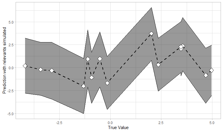
(a) Predictions

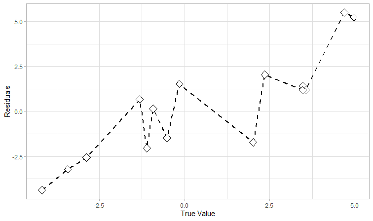
(b) Residuals

Figure 4: Conformal prediction with simulated relevant controls and OLS

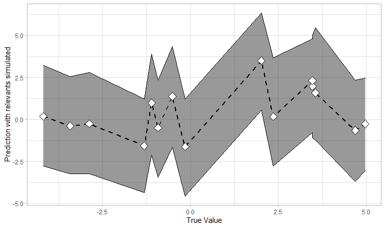
(a) Predictions

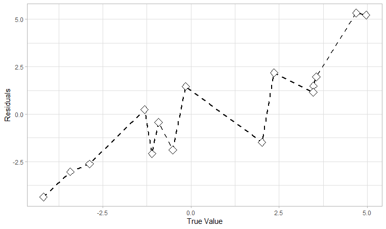
(b) Residuals

Figure 5: Conformal prediction with simulated relevant controls and LASSO

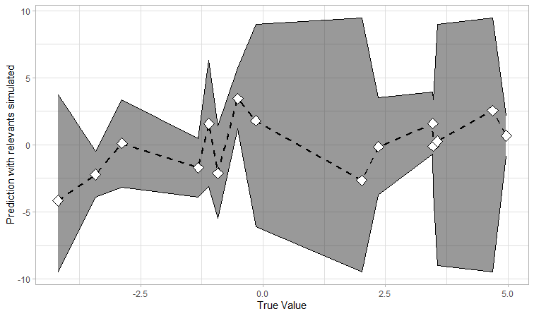
(a) Predictions

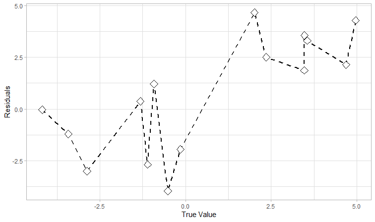
(b) Residuals

Figure 6: Conformal prediction with simulated relevant controls and Kernel regression

Figure 7 is obtained using the smaller dataset to show the comparison among the three conformal prediction methods. We can see that they do not differ much for the three values used as queries.

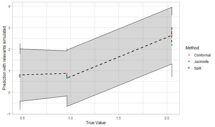
(a) Predictions

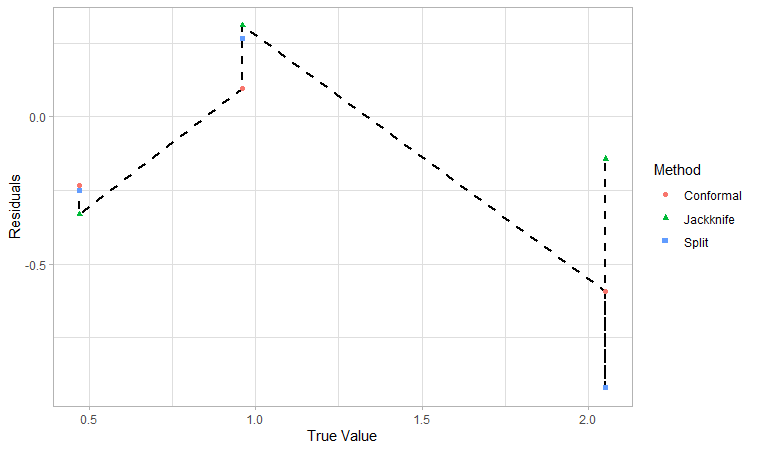
(b) Residuals

Figure 7: Results of the three methods with simulated relevant controls and LASSO

5 Discussion

As already noted, the intervals adapt to each query. The point forecasts depend more on the data used than on the method of conformal prediction chosen. The prediction of the point values tends to be very conservative and thus the residuals become negative on the left and positive on the right. In most cases the predicted intervals capture the true values.

The cases analyzed empirically here are, of course, very simple. They do not allow us to explore exhaustively all the consequences of the choices at the initialization phase of Algorithm 1. But we can make the preliminary observation that no clear winner can be ascertained among the conformal prediction method, since the three variants yield in average similar results, although the split conformal one is less computationally costly.

Our method yields adaptive intervals using only relevant plus simulated data as to ensure the robustness of the predictions. This divide and conquer strategy is particularly appropriate for large and heterogeneous datasets. Subsets of data individualize the forecasts of variables of which specific information is not available.

As an extra bonus, for each query we obtain a distribution of relevant data. This captures a latent variable (this facilitates the prediction of the intervals corresponding to the query), providing useful information about the individuals in the same “class”.

On the downside, we have seen that residuals are more widely dispersed at the tails of the distribution of actual values. This is inherited from the application of conformal methods, unlike in the self-supervised method of Seedat et al., (2023), where residuals are used to train the system to improve its predictions.

Further work is needed to make a more precise assessment of the pros and cons of the method, enriching it by relating it to other procedures presented in the literature. Possible lines of study are:

• Run more experiments using a larger $p$ or a higher-dimensional setup.

• Marginalize the individual result up from that of the the relevant group (or even up from the group of non-relevant ones) as in Zhou et al., (2023).

• Explore whether our individualization strategy is compatible with the version of divide and conquer discussed in Chen et al., (2021).

• Use residuals to create corrections at the tails of the intervals as to reduce the epistemic uncertainty at the boundaries Alaa et al., (2023).

Appendix

Setting $A$	Setting $B$	Setting $C$
one variable	two variables	heteroskedastic
$n_{1}=250$	$n_{2}=250$	$n_{3}=250$
$u_{1}=\mbox{rnorm}(n_{1})$	$u_{2}=\mbox{rnorm}(n_{2})$	$x_{1c}=\mbox{rnorm}(n_{3},1,1)$
$x_{1a}=\mbox{rnorm}(n_{1},1,1)$	$x_{1b}=\mbox{rnorm}(n_{2},3,1)$	$u_{3}=\mbox{rnorm}(n_{3})*\frac{x_{1c}}{2}$
$x_{2a}=\mbox{rnorm}(n_{1},2,1)$ (irrelevant)	$x_{2b}=\mbox{rnorm}(n_{2},2,2)$	$x_{2c}=\mbox{rnorm}(n_{3},3,2)$
$y_{a}=0.5*x_{1a}+u_{1}$	$y_{b}=0.5*x_{1b}+0.33*x_{2b}+u_{2}$	$y_{c}=0.5*x_{1c}*x_{1c}+0.33*x_{2c}+u_{3}$
new data for $A$	new data for $B$	new data for $C$
$x_{01a}=\mbox{rnorm}(1,1,1)$	$x_{01b}=\mbox{rnorm}(1,3,1)$	$x_{01c}=\mbox{rnorm}(1,1,1)$
$x_{02a}=\mbox{rnorm}(1,2,2)$	$x_{02b}=\mbox{rnorm}(1,2,2)$	$x_{02c}=\mbox{rnorm}(1,3,2)$
$y_{0a}=0.5*x_{01a}$	$y_{0b}=0.5*x_{01b}+0.33*x_{02b}$	$y_{0c}=0.5*x_{01c}+0.33*x_{02c}$
$+$ $\mbox{rnorm}(1)$	$+$ $\mbox{rnorm}(1)$	$+$ $\mbox{rnorm}(1)*\frac{x_{01c}}{2}$

Table 1: Simulation datasets with large $n$ and small $p$ (using functions from the R language)

$DGP_{1}$:	$DGP_{2}$:	$DGP_{3}$:
12 variables $N(0,1)$ with 2 coefficients $=0$	shift in the mean of the features	shift in the mean of the coefficients
$n_{1}=100;p_{1}=12;s_{1}=2$	$n_{2}=100;p_{2}=12;s_{2}=2$	$n_{3}=100;p_{3}=12;s_{3}=2$
$x_{1}=\mbox{matrix}(\mbox{rnorm}(n_{1}*p_{1}),n_{1},p_{1})$	$x_{2}=\mbox{matrix}(\mbox{rnorm}(n_{2}*p_{2},\mbox{mean}=1),n_{2},p_{2})$	$x_{3}=\mbox{matrix}(\mbox{rnorm}(n_{3}*p_{3}),n_{3},p_{3})$
$\beta_{1}=\mbox{c}(\mbox{rnorm}(s_{1}),\mbox{rep}(0,p_{1}-s_{1}))$	$\beta_{2}=\mbox{c}(\mbox{rnorm}(s_{2}),\mbox{rep}(0,p_{2}-s_{2}))$	$\beta_{3}=\mbox{c}(\mbox{rnorm}(s_{3},\mbox{mean}=1),\mbox{rep}(0,p_{3}-s_{3}))$
$y_{1}=x_{1}*\beta_{1}+\mbox{rnorm}(n_{1})$	$y_{2}=x_{2}*\beta_{2}+\mbox{rnorm}(n_{2})$	$y_{3}=x_{3}*\beta_{3}+\mbox{rnorm}(n_{3})$
$n_{01}=5$	$n_{02}=5$	$n_{03}=5$
$x_{01}=\mbox{matrix}(\mbox{rnorm}(n_{01}*p_{1}),n_{01},p_{1})$	$x_{02}=\mbox{matrix}(\mbox{rnorm}(n_{02}*p_{2},\mbox{mean}=1),n_{02},p_{2})$	$x_{03}=\mbox{matrix}(\mbox{rnorm}(n_{03}*p_{3}),n_{03},p_{3})$
$y_{01}=x_{01}*\beta_{1}+\mbox{rnorm}(n_{01})$	$y_{02}=x_{02}*\beta_{2}+\mbox{rnorm}(n_{02})$	$y_{03}=x_{03}*\beta_{3}+\mbox{rnorm}(n_{03})$
$D_{1}=\mbox{as.data.frame}(\mbox{cbind}(y_{1},x_{1}))$	$D_{2}=\mbox{as.data.frame}(\mbox{cbind}(y_{2},x_{2}))$	$D_{3}=\mbox{as.data.frame}(\mbox{cbind}(y_{3},x_{3}))$
$x_{1}=\mbox{as.data.frame}(x_{1})$	$x_{2}=\mbox{as.data.frame}(x_{2})$	$x_{3}=\mbox{as.data.frame}(x_{3})$

Table 2: Simulation datasets with smaller $n$ and large $p$ (using functions from the R language)

Cosine	Confomal			Split			Jackknife
variable	$1$	$2$	$3$	$1$	$2$	$3$	$1$	$2$	$3$
y0	$0.96$	$2.05$	$0.47$	$0.96$	$2.05$	$0.47$	$0.96$	$2.05$	$0.47$
pred	$0.96$	$2.59$	$0.95$	$0.96$	$2.79$	$0.9$	$2.06$	$0.71$	$0.98$
predr	$0.88$	$2.43$	$0.84$	$0.79$	$2.81$	$0.75$	$0.67$	$2.19$	$0.84$
predrs	$0.88$	$2.41$	$0.84$	$0.91$	$2.63$	$0.9$	$0.69$	$2.2$	$0.8$
predl	$0.96$	$2.59$	$0.95$	$0.96$	$2.59$	$0.95$	$2.05$	$0.71$	$0.99$
predlr	$0.88$	$2.43$	$0.84$	$0.79$	$2.81$	$0.75$	$0.64$	$2.08$	$0.78$
predlrs	$0.9$	$2.47$	$0.86$	$0.91$	$2.63$	$0.9$	$0.65$	$2.19$	$0.8$
lo	$-0.36$	$1.36$	$-0.36$	$-0.83$	$1.01$	$-0.89$	$0.22$	$-1.13$	$-0.85$
lor	$0.65$	$0.79$	$1.08$	$-1.28$	$0.36$	$-0.88$	$-0.73$	$0.59$	$-0.48$
lors	$-0.36$	$1.08$	$-0.36$	$-0.59$	$0.49$	$-0.08$	$-0.63$	$0.71$	$-0.42$
lol	$-0.36$	$1.36$	$-0.36$	$-0.81$	$0.83$	$-0.81$	$0.22$	$-1.12$	$-0.84$
lolr	$0.5$	$0.79$	$1.08$	$-1.28$	$0.37$	$-0.88$	$-0.73$	$-0.41$	$-0.62$
lolrs	$-0.36$	$1.08$	$-0.36$	$-0.59$	$0.49$	$-0.08$	$-0.67$	$0.71$	$-0.42$
up	$2.22$	$3.8$	$2.22$	$2.74$	$4.58$	$2.69$	$3.89$	$2.54$	$2.82$
upr	$3.08$	$3.51$	$3.51$	$2.96$	$4.52$	$2.39$	$2.08$	$3.79$	$2.15$
uprs	$2.08$	$3.8$	$2.08$	$2.39$	$4.51$	$1.88$	$2$	$3.69$	$2.03$
upl	$2.22$	$3.8$	$2.22$	$2.72$	$4.36$	$2.71$	$3.88$	$2.54$	$2.82$
uplr	$3.08$	$3.51$	$3.51$	$2.96$	$4.53$	$2.39$	$2$	$4.57$	$2.19$
uplrs	$2.22$	$3.8$	$2.08$	$2.39$	$4.51$	$1.88$	$1.95$	$3.57$	$2.01$

Table 3: Cosine Relevance

Note: pred, lo and up denote the prediction, lower limit and upper limit of the interval, respectively. In turn, r correspond to the case when only relevant observations are used while rs appears in cases in which both relevant and simulated observations are included. Finally, l and k refer to the cases in which LASSO regressions and kernel estimations are used, respectively.

Percentile	Confomal			Split			Jackknife
variable	$1$	$2$	$3$	$1$	$2$	$3$	$1$	$2$	$3$
y0	$0.96$	$2.05$	$0.47$	$0.96$	$2.05$	$0.47$	$0.96$	$2.05$	$0.47$
pred	$0.96$	$2.59$	$0.95$	$0.96$	$2.79$	$0.9$	$2.06$	$0.71$	$0.98$
predr	$0.84$	$2.57$	$0.69$	$0.43$	$2.05$	$0.58$	$0.67$	$2.19$	$0.84$
predrs	$0.86$	$2.56$	$0.68$	$0.7$	$2.97$	$0.72$	$0.69$	$2.2$	$0.8$
predl	$0.96$	$2.59$	$0.95$	$0.96$	$2.59$	$0.95$	$2.05$	$0.71$	$0.99$
predlr	$0.84$	$2.57$	$0.69$	$0.43$	$2.02$	$0.58$	$0.64$	$2.08$	$0.78$
predlrs	$0.87$	$2.64$	$0.7$	$0.7$	$2.97$	$0.72$	$0.65$	$2.19$	$0.8$
lo	$-0.36$	$1.36$	$-0.36$	$-0.34$	$1.5$	$-0.39$	$0.22$	$-1.13$	$-0.85$
lor	$0.76$	$0.97$	$-0.28$	$-0.21$	$1.25$	$-0.59$	$-0.73$	$0.59$	$-0.48$
lors	$-0.25$	$1.2$	$-0.41$	$-0.34$	$0.88$	$-0.79$	$-0.63$	$0.71$	$-0.42$
lol	$-0.36$	$1.36$	$-0.36$	$-0.31$	$1.33$	$-0.32$	$0.22$	$-1.12$	$-0.84$
lolr	$1.05$	$1.2$	$-0.47$	$-0.26$	$1.25$	$-0.6$	$-0.73$	$-0.41$	$-0.62$
lolrs	$-0.18$	$1.31$	$-0.41$	$-0.34$	$0.88$	$-0.79$	$-0.67$	$0.71$	$-0.42$
up	$2.22$	$3.8$	$2.22$	$2.25$	$4.09$	$2.19$	$3.89$	$2.54$	$2.82$
upr	$2.92$	$3.49$	$1.91$	$2.1$	$4.09$	$1.75$	$2.08$	$3.79$	$2.15$
uprs	$1.91$	$3.94$	$1.79$	$2$	$3.9$	$2.24$	$2$	$3.69$	$2.03$
upl	$2.22$	$3.8$	$2.22$	$2.22$	$3.86$	$2.21$	$3.88$	$2.54$	$2.82$
uplr	$3.29$	$3.83$	$1.72$	$2.17$	$4.09$	$1.76$	$2$	$4.57$	$2.19$
uplrs	$1.91$	$3.94$	$1.79$	$2$	$3.9$	$2.24$	$1.95$	$3.57$	$2.01$

Table 4: Percentile relevance

Note: Here we use the same abbreviations as in table 3

Short data
Percentile	General	Conformal	Split	Jackknife
diffpred	0.57	0.34	0.39	0.98
diffpredr	0.25	0.28	0.21	0.26
diffpredrs	0.33	0.27	0.48	0.25
diffpredl	0.55	0.34	0.34	0.98
diffpredlr	0.24	0.28	0.22	0.22
diffpredlrs	0.35	0.31	0.48	0.26
diffpredk	0.32	0.3	0.31	0.34
diffpredkr	0.24	0.2	0.24	0.28
diffpredkrs	0.25	0.19	0.27	0.28
%pred	60.25	42.49	42.38	95.87
%predr	30.52	27.57	26.09	37.92
%predrs	34.42	26.03	41.81	35.41
%predl	60.31	42.49	42.56	95.89
%predlr	29.28	27.57	26.65	33.62
%predlrs	35.9	29.26	41.91	36.54
%predk	38.37	36.05	36.49	42.58
%predkr	26.22	23.44	27.83	27.39
%predkrs	27.79	23.29	32.62	27.45
int	2.93	2.53	2.59	3.67
intr	2.56	2.29	2.49	2.89
intrs	2.62	2.37	2.8	2.69
intl	2.91	2.53	2.53	3.66
intlr	2.8	2.35	2.54	3.5
intlrs	2.58	2.31	2.8	2.64
intk	2.56	2.53	2.49	2.65
intkr	2.95	2.56	2.61	3.66
intkrs	2.45	2.29	2.65	2.41
ab	0.6	0.63	0.65	0.52
abr	0.61	0.71	0.59	0.53
abrs	0.55	0.58	0.55	0.53
abl	0.6	0.63	0.63	0.52
ablr	0.62	0.76	0.59	0.5
ablrs	0.55	0.59	0.55	0.51
abk	0.62	0.61	0.62	0.63
abkr	0.57	0.63	0.54	0.55
abkrs	0.54	0.54	0.51	0.58

Table 5: Short data percentile

Note: diffpred denotes the differences between the predicted and the true values. %pred indicates the same difference but relative to the true value. int is the length of the interval (the upper minus the lower limits). Finally, ab represents the size of the error relative to the length of the interval.

Short data
Cosine	General	Conformal	Split	Jackknife
diffpred	0.57	0.34	0.39	0.98
diffpredr	0.31	0.28	0.4	0.26
diffpredrs	0.29	0.27	0.35	0.25
diffpredl	0.55	0.34	0.34	0.98
diffpredlr	0.3	0.28	0.4	0.22
diffpredlrs	0.3	0.29	0.35	0.26
diffpredk	0.32	0.3	0.34	0.31
diffpredkr	0.6	0.8	0.57	0.44
diffpredkrs	0.93	1.1	0.58	1.11
%pred	60.25	42.49	42.38	95.87
%predr	37.08	35.18	38.15	37.92
%predrs	37.27	34.79	41.6	35.41
%predl	60.31	42.49	42.56	95.89
%predlr	35.65	35.18	38.15	33.62
%predlrs	38.18	36.4	41.6	36.54
%predk	38.41	36.05	42.7	36.49
%predkr	89.13	102.14	99.06	66.2
%predkrs	144.67	153.04	99.05	181.92
int	3.26	2.53	3.58	3.67
intr	3.1	2.53	3.89	2.89
intrs	2.74	2.53	2.99	2.69
intl	3.24	2.53	3.52	3.66
intlr	3.33	2.58	3.89	3.5
intlrs	2.74	2.58	2.99	2.64
intk	2.56	2.53	2.64	2.49
intkr	2.93	2.86	3.41	2.52
intkrs	2.91	3.37	2.68	2.67
ab	0.59	0.63	0.61	0.52
abr	0.65	0.88	0.55	0.53
abrs	0.57	0.59	0.6	0.53
abl	0.58	0.63	0.6	0.52
ablr	0.64	0.87	0.55	0.5
ablrs	0.57	0.6	0.6	0.51
abk	0.62	0.61	0.63	0.62
abkr	0.62	0.37	0.54	0.94
abkrs	0.73	0.62	0.58	0.99

Table 6: Short data cosine

Note: Here we use the same abbreviations as in table 5

Long data
Cosine	General	Conformal	Split	Jackknife
diffpred	2.8	2.47	2.58	3.34
diffpredr	2.75	2.27	2.64	3.34
diffpredrs	2.8	2.29	2.76	3.34
diffpredl	2.81	2.48	2.6	3.35
diffpredlr	2.73	2.29	2.61	3.28
diffpredlrs	2.78	2.34	2.69	3.33
diffpredk	2.05	1.5	2.32	2.33
diffpredkr	1.91	1.7	1.87	2.17
diffpredkrs	2.1	1.77	2.39	2.14
%pred	179.03	165.13	105.96	266.02
%predr	168.86	157.93	115.92	232.74
%predrs	183.81	157.16	165.13	229.12
%predl	176.34	165.17	98.11	265.75
%predlr	173.31	135.75	109.4	274.78
%predlrs	174.9	160.28	136.48	227.92
%predk	161.98	132.38	183.64	169.93
%predkr	131.49	166.7	109.41	118.35
%predkrs	154.95	126.67	215.02	123.15
int	5.13	5.86	5.96	3.57
intr	5.03	5.51	5.95	3.64
intrs	4.31	5.87	3.52	3.54
intl	5.14	5.69	6.38	3.36
intlr	6.78	5.76	6.24	8.33
intlrs	4.31	5.94	3.52	3.48
intk	5.43	4.12	6.71	5.45
intkr	6.05	5.27	5.58	7.31
intkrs	5.97	1.77	9.41	6.73
ab	0.6	0.42	0.43	0.94
abr	0.59	0.41	0.45	0.92
abrs	0.71	0.39	0.8	0.94
abl	0.61	0.44	0.41	1
ablr	0.41	0.4	0.42	0.4
ablrs	0.75	0.39	0.78	1.09
abk	0.38	0.36	0.35	0.43
abkr	0.33	0.33	0.35	0.3
abkrs	0.63	1.21	0.36	0.32

Table 7: Long data cosine

Note: Here we use the same abbreviations as in table 5

References

- Alaa et al., (2023) Alaa, A. M., Hussain, Z., and Sontag, D. (2023). Conformalized unconditional quantile regression. arXiv preprint arXiv:2304.01426.
- Alaa and Van Der Schaar, (2017) Alaa, A. M. and Van Der Schaar, M. (2017). Bayesian inference of individualized treatment effects using multi-task gaussian processes. Advances in neural information processing systems, 30.
- Barber et al., (2021) Barber, R. F., Candes, E. J., Ramdas, A., and Tibshirani, R. J. (2021). Predictive inference with the jackknife+. The Annals of Statistics, 49(1):486–507.
- Cai et al., (2021) Cai, C., Chen, R., and Xie, M.-g. (2021). Individualized group learning. Journal of the American Statistical Association, pages 1–17.
- Chen et al., (2021) Chen, X., Cheng, J. Q., and Xie, M.-g. (2021). Divide-and-conquer methods for big data analysis. arXiv preprint arXiv:2102.10771.
- Chernozhukov et al., (2017) Chernozhukov, V., Chetverikov, D., Demirer, M., Duflo, E., Hansen, C., and Newey, W. (2017). Double/debiased/neyman machine learning of treatment effects. American Economic Review, 107(5):261–65.
- Delbianco et al., (2021) Delbianco, F., Fioriti, A., and Tohmé, F. (2021). A methodology to answer to individual queries: finding relevant and robust controls. Behaviormetrika, 48(2):259–282.
- Infanger and Schmidt-Trucksäss, (2019) Infanger, D. and Schmidt-Trucksäss, A. (2019). P value functions: An underused method to present research results and to promote quantitative reasoning. Statistics in Medicine, 38(21):4189–4197.
- Kuhn, (2008) Kuhn, M. (2008). Building predictive models in r using the caret package. Journal of statistical software, 28:1–26.
- Lei et al., (2018) Lei, J., G’Sell, M., Rinaldo, A., Tibshirani, R. J., and Wasserman, L. (2018). Distribution-free predictive inference for regression. Journal of the American Statistical Association, 113(523):1094–1111.
- Li and Meng, (2021) Li, X. and Meng, X.-L. (2021). A multi-resolution theory for approximating infinite-p-zero-n: Transitional inference, individualized predictions, and a world without bias-variance tradeoff. Journal of the American Statistical Association, 116(533):353–367.
- Meng, (2018) Meng, X.-L. (2018). Statistical paradises and paradoxes in big data (i) law of large populations, big data paradox, and the 2016 us presidential election. The Annals of Applied Statistics, 12(2):685–726.
- Schweder and Hjort, (2016) Schweder, T. and Hjort, N. L. (2016). Confidence, likelihood, probability, volume 41. Cambridge University Press.
- Seedat et al., (2023) Seedat, N., Jeffares, A., Imrie, F., and van der Schaar, M. (2023). Improving adaptive conformal prediction using self-supervised learning. arXiv preprint arXiv:2302.12238.
- Shen et al., (2018) Shen, J., Liu, R. Y., and Xie, M.-g. (2018). Prediction with confidence—a general framework for predictive inference. Journal of Statistical Planning and Inference, 195:126–140.
- Shen et al., (2020) Shen, J., Liu, R. Y., and Xie, M.-g. (2020). i fusion: Individualized fusion learning. Journal of the American Statistical Association, 115(531):1251–1267.
- Tran et al., (2017) Tran, T., Pham, T., Carneiro, G., Palmer, L., and Reid, I. (2017). A bayesian data augmentation approach for learning deep models. Advances in neural information processing systems, 30.
- Vovk et al., (2022) Vovk, V., Gammerman, A., and Shafer, G. (2022). Algorithmic learning in a random world. Springer.
- Xie and Singh, (2013) Xie, M.-g. and Singh, K. (2013). Confidence distribution, the frequentist distribution estimator of a parameter: A review. International Statistical Review, 81(1):3–39.
- Xie and Wang, (2022) Xie, M.-g. and Wang, P. (2022). Repro samples method for finite-and large-sample inferences. arXiv preprint arXiv:2206.06421.
- Xie and Zheng, (2022) Xie, M.-g. and Zheng, Z. (2022). Homeostasis phenomenon in conformal prediction and predictive distribution functions. International Journal of Approximate Reasoning, 141:131–145.
- Zhou et al., (2023) Zhou, Z., Li, D., Huh, D., Xie, M., and Mun, E.-Y. (2023). A simulation study of the performance of statistical models for count outcomes with excessive zeros: Focusing on the marginalized model. arXiv preprint arXiv:2301.12674.