Approaching Test Time Augmentation in the Context of Uncertainty Calibration for Deep Neural Networks

Abstract

With the rise of Deep Neural Networks, machine learning systems are nowadays ubiquitous in a number of real-world applications, which bears the need for highly reliable models. This requires a thorough look not only at the accuracy of such systems, but also to their predictive uncertainty. Hence, we propose a novel technique (with two different variations, named M-ATTA and V-ATTA) based on test time augmentation, to improve the uncertainty calibration of deep models for image classification. Unlike other test time augmentation approaches, M/V-ATTA improves uncertainty calibration without affecting the model’s accuracy, by leveraging an adaptive weighting system. We evaluate the performance of the technique with respect to different metrics of uncertainty calibration. Empirical results, obtained on CIFAR-10, CIFAR-100, as well as on the benchmark Aerial Image Dataset, indicate that the proposed approach outperforms state-of-the-art calibration techniques, while maintaining the baseline classification performance. Code for M/V-ATTA available at: https://github.com/pedrormconde/MV-ATTA

1 Introduction

Deep Neural Networks (DNNs) changed the paradigm with regards to the applicability of machine learning (ML) systems to real-world scenarios. Consequently, deep learning (DL) models are now present in critical application domains (e.g., autonomous driving, medicine, remote sensing, robotics), where bad decision-making can bear potentially drastic consequences. This requires that DNNs are not only highly accurate, but also highly reliable - decision-makers should be able to “trust” the predictions of these models. This lead us to the problem of uncertainty calibration (also referred as confidence calibration or simply calibration): it is required that the confidence output generated by the DL model - that translates as the confidence the model has in the prediction that is making - realistically represents the true likelihood of correctness. For the sake of intuition, a calibrated model would for example, in the long run, correctly classify $70\%$ of those predictions that have a confidence value of $0.7$ associated. This accurate quantification of predictive uncertainty results in reliable confidence values associated with each prediction, and therefore, in a more reliable model. As such, it is important to understand how well calibrated are modern DNNs. Further details, including the formalization of the uncertainty calibration problem, will be described in Section 3.
Although increasingly accurate, modern DL architectures have been found to be tendentiously uncalibrated [7, 20]. Furthermore, “modern neural networks exhibit a strange phenomenon: probabilistic error and miscalibration worsen even as classification error is reduced” [7]. For this reason, the goal of this work is to improve the uncertainty calibration of DNNs in the task of image classification, by proposing a novel accuracy-consistent weighted test time augmentation method.
Test time augmentation is a general methodology that leverages data augmentation techniques to create multiple samples from the original input at inference (i.e., at test time). Therefore, test time augmentation methods can be applied to pre-trained models, since, in this case, the augmentation process is not applied during the training phase. The technique introduced in this work combines the use of test time augmentation with a custom weighting system, guaranteeing that the accuracy of the original DL model is not corrupted, while still being optimized to improve uncertainty calibration. This builds, partially, on the work done in [3], proposing both a reformulated version - V-ATTA (Vector Adaptive Test Time Augmentation) - of the preliminary method presented in [3] and also a generalized version - M-ATTA (Matrix Adaptive Test Time Augmentation) - with a broader and extended empirical evaluation.
M/V-ATTA is evaluated on the benchmark CIFAR-10/CIFAR-100 [11] datasets, as well as on a benchmark satellite imagery dataset, the Aerial Image Dataset (AID) [28]. The results are compared with state-of-the-art post-hoc calibration methods, with respect to the Brier score [2] and the Expected Calibration Error (ECE), for both common and strong uncertainty calibration (see Section 3 for further details).
Contribution: We propose a novel calibration technique - with two different variations (M/V-ATTA) - based on test time augmentation, that guarantees consistency in the accuracy of deep models in which is applied, while being shown to improve uncertainty calibration-related evaluation metrics, outperforming state-of-the-art post-hoc calibration methods in most cases. To the best of our knowledge, M/V-ATTA is the first method based on test time augmentation that has been proposed to improve the uncertainty calibration of deep models (besides its predecessor in [3]). Furthermore, the method presented here can be used with pre-trained DNNs, which is advantageous in terms of applicability.

2 Related Work

The authors in [7] introduce the topic of uncertainty calibration to the DL community, by evaluating how well calibrated are different modern DNNs, using different datasets (from both computer vision and natural language processing applications). As previously stated, the authors argue that, although more accurate, modern DNNs exhibit problems of miscalibration, often more severe than those found in older - and less accurate - architectures. Several post-hoc calibration techniques - particularly designed to address uncertainty calibration without the need of re-training the original DL models - like temperature scaling (an extension of the Platt scaling algorithm [22, 18]), histogram binning [29] and isotonic regression [30], are described to address this problem.
Other approaches, like approximate Bayesian models [6, 4] and some regularization techniques [21, 15], have also been used in the context of uncertainty calibration [20]. Nonetheless, these approaches require building new more complex models or modifying and re-training pre-existing ones, contrarily to the previously mentioned post-hoc calibration methods and the proposed M/V-ATTA.
For the evaluation of uncertainty calibration, one of the most popular metrics is the ECE [17], where the bin-wise difference between the accuracy and the confidence outputs of a given model is evaluated. Although intuitive, some limitations of this metric have been identified in relevant literature [19, 8, 27], with regard to, for example, its intractability and dependence on the chosen binning scheme. Furthermore, because ECE is not a proper scoring rule [5], there can be found trivial uninformative solutions that obtain an optimal score, like always returning the marginal probability (see example in Supplementary Material, Section 2). A popular alternative to evaluate uncertainty calibration is the Brier score [2]; because it is a proper scoring rule and overcomes some of the identified limitation of the ECE, this metric has been increasingly used by the scientific community [20, 24, 13].
Test time augmentation methods have been gaining some attention in the last few years, for example in biomedical applications [26, 25, 14]. Nonetheless, we see that some potential in this type of technique is still under-researched and, to the best of our knowledge, all relevant literature fails to address its effect on calibration-specific metrics like the Brier score or the ECE (with exception of our preliminary work done in [3]). Contrarily to other recent novel approaches to test time augmentation [12, 10, 23], the method proposed in this work does not focuses on improving the accuracy of DNNs, but instead on improving their uncertainty calibration without altering the original accuracy. In fact, the authors in [23] show that some forms of test time augmentation may produce corrupted predictions - which can ultimately worsen the model’s performance - reinforcing the need for a test time augmentation-based methodology that does not alter the predicted class, while still calibrating its confidence value.

3 Background

Notation: we will use bold notation to denote vectors, like $\mathbf{p}=~{}(p_{1},\ldots,p_{k})$; the $i$-nth element of some vector $\mathbf{p}$ will be referred as $\mathbf{p}_{\{i\}}:=p_{i}$; the $\downarrow$ symbol, associated with a given metric, informs that a lower value of such metric represents a better performance; the $\odot$ symbol represents the Hadamard product, $\sigma:\mathbb{R}^{k}\rightarrow\Delta_{k}$ represents the softmax function. These remarks are valid for all sections of the article; other remarks on notation will be given along the text, when found relevant.

In this section we discuss the problem of uncertainty calibration and present some evaluation metrics commonly used in this context. In relevant literature, the concept of uncertainty calibration related to DL systems in a multi-class scenario is often defined in two different ways. The most common way is the one presented in [7], where the multi-class scenario is considered as an extension of the binary problem in a one vs all approach, taking in account only the calibration of the highest confidence value for each prediction. Nonetheless, some works consider the more general definition present in [29], that takes into account all the confidence values of the predicted probability vector. Like in [27], we make the respective distinction between a calibrated model and a strongly calibrated model, in the following definitions. Notice that in the case of a binary classifier such definitions are equivalent.
Let us consider a pair of random variables $(X,Y)$, where $X$ represents an input space (or feature space) and $Y$ the corresponding set of true labels. Let us now take a model $f:X\rightarrow\Delta_{k}$, with $\Delta_{k}=~{}\{(p_{1},\ldots,p_{k})\in[0,1]^{k}:\sum_{i=1}^{k}p_{i}=1\}$ being a probability simplex (this setting corresponds to a classification problem with $k$ different classes). The model $f$ is considered calibrated if

$$\mathds{P}[Y=\operatorname*{arg\,max}_{i\in\{1,\ldots,k\}}f(X)\ |\ \max_{i\in\{1,\ldots,k\}}f(X)]=\max_{i\in\{1,\ldots,k\}}f(X).$$ (1)

Additionally, the model $f$ is considered strongly calibrated if

$$\mathds{P}[Y=y\ |\ f(X)_{\{y\}}]=f(X)_{\{y\}}.$$ (2)

As stated in [7], achieving perfect calibration is impossible in practical settings. Furthermore, the probability values in the left hand side of both (1) and (2) cannot be computed using finitely many samples, which motivates the need for scoring rules to assess uncertainty calibration.

3.1 Brier score $\downarrow$

Brier score [2] is a proper scoring rule [5] that computes the squared error between a predicted probability and its true response, hence its utility to evaluate uncertainty calibration. For a set of $N$ predictions we define the Brier score as

$$\text{BS}=\frac{1}{N}\sum_{j=1}^{N}(p^{j}-o^{j})^{2},$$ (3)

where $p^{j}$ is the highest confidence value of the prediction $j$ and $o^{j}$ equals 1 if the true class corresponds to the prediction and 0 otherwise.

The previous definition is useful to asses calibration (in the more common sense). Nonetheless, [2] also presents a definition for Brier score in multi-class scenario that is suitable to assess strong calibration. For a problem with $k$ different classes and a set of $N$ predictions we define the multi-class Brier score (mc-Brier score) as

$$\text{mc-BS}=\frac{1}{N}\sum_{j=1}^{N}\sum_{i=1}^{k}(p_{i}^{j}-o_{i}^{j})^{2},$$ (4)

where $p_{i}^{j}$ is the confidence value in the position $i$ of the $j$-nth prediction probability vector and $o_{i}^{j}$ equals 1 if the true label equals $i$ and 0 otherwise.
We refer to [16] and [1] for some thorough insights about the interpretability and decomposition of the Brier score.

3.2 Expected Calibration Error $\downarrow$

To compute the ECE [17] we start by dividing the interval $[0,1]$ in $M$ equally spaced intervals. Then a set of bins $\{B_{1},B_{2},\ldots,B_{M}\}$ is created, by assigning each predicted probability value to the respective interval. The idea behind this measurement is to compute a weighted average of the absolute difference between accuracy and confidence in each bin $B_{i}$ ($i=1,\ldots,M$). We define the confidence per bin as

$$conf(B_{i})=\frac{1}{|B_{i}|}\sum_{j\in B_{i}}p^{j},$$ (5)

where $p^{j}$ is the highest confidence value of the prediction $j$. The accuracy per bin is defined as

$$acc(B_{i})=\frac{1}{|B_{i}|}\sum_{j\in B_{i}}o^{j},$$ (6)

where $o^{j}$ equals 1 if the true class corresponds to the prediction and 0 otherwise. For a total of $N$ predictions and a binning scheme $\{B_{1},B_{2},\ldots,B_{M}\}$, the ECE is defined as

$$\text{ECE}=\sum_{i=1}^{M}\frac{|B_{i}|}{N}|conf(B_{i})-acc(B_{i})|.$$ (7)

4 Proposed Methodology

In this section we introduce M-ATTA and V-ATTA. Both methods leverage the use of test time augmentation, combined with a custom adaptive weighting system. V-ATTA can be interpreted as restricted version of the more general M-ATTA.

1

Input: Augmented logits matrix ($\mathbf{Z}\in\mathbb{R}^{k,m}$), Original prediction ($\mathbf{p}^{0}\in\Delta_{k}$)

2

Output: Calibrated prediction ($\mathbf{p}\in\Delta_{k}$)

Learnable parameters: $\mathbf{W}\in\mathbb{R}^{k,m}$, $\omega^{*}\in\mathbb{R}$

3

4$\epsilon\leftarrow 0.01$

5$\tilde{\omega}\leftarrow\omega^{*}$

6$c_{0}\leftarrow\operatorname*{arg\,max}_{i\in\{1,\ldots,k\}}\mathbf{p}^{0}$

7while $c\neq c_{0}\ \land\ \tilde{\omega}>0$ do

8      

9      $\mathbf{p}\leftarrow(1-\tilde{\omega})\mathbf{p}^{0}+\tilde{\omega}\text{ }\sigma(\mathbf{W}\odot\mathbf{Z})I_{m}$

10      $c\leftarrow\operatorname*{arg\,max}_{i\in\{1,\ldots,k\}}\mathbf{p}$

11      $\tilde{\omega}\leftarrow\tilde{\omega}-\epsilon$

Algorithm 1 M-ATTA

4.1 M-ATTA

Let us start by considering $m\in\mathbb{N}$ different types of augmentations. Because it is common that some augmentations have random parameters, it can be desirable to apply the same type of augmentation more than once; for this reason, let us consider as $n_{i}$ ($i=1,\ldots,m$) the number of times the $i$-nth type of augmentation is applied. As such, we will define for each original input $I_{0}$, the $j$-nth ($j=1,\ldots,n_{i}$) augmented input with the $i$-nth augmentation type, as $I_{i,j}$.
We can now take into account the model $f:X\rightarrow\Delta_{k}$ (where $X$ is the input space and $k$ the number of classes) and consider $g:X\rightarrow\mathbb{R}^{k}$ as such that $f:=g\circ\sigma$ . With this, we now define

$$p^{0}=f(I_{0}),\qquad z_{i,j}=g(I_{i,j}),$$ (8)

i.e., $p^{0}$ is the probability vector associated with the original input and $z_{i,j}$ is the logit associated with the $j$-nth augmentation of the $i$-nth type. Subsequently, we can define, $\forall i\in[1,\ldots,m]$,

$$\mathbf{z}^{i}=\frac{\sum_{j=1}^{n_{i}}\mathbf{z}_{i,j}}{n_{i}}\equiv\left(z^{i}_{1},z^{i}_{2},\ldots,z^{i}_{k}\right)\in\mathbb{R}^{k},$$ (9)

and then construct the matrix

$$\mathbf{Z}=\left[\mathbf{z}^{i}\right]_{i=1,\ldots,m}^{\text{T}}=\left[\begin{array}[]{ccccc}z^{1}_{1}&z^{2}_{1}&\cdots&z^{m}_{1}\vskip 6.0pt plus 2.0pt minus 2.0pt\\ z^{1}_{2}&z^{2}_{2}&\cdots&z^{m}_{2}\\ \vdots&\vdots&\ddots&\vdots\\ z^{1}_{k}&z^{2}_{k}&\cdots&z^{m}_{k}\end{array}\right]\in\mathbb{R}^{k,m}.$$ (14)

Now, for some parameters

$$\omega^{*}\in[0,1],\quad\mathbf{W}=\left[\begin{array}[]{ccccc}\omega^{1}_{1}&\omega^{2}_{1}&\cdots&\omega^{m}_{1}\vskip 6.0pt plus 2.0pt minus 2.0pt\\ \omega^{1}_{2}&\omega^{2}_{2}&\cdots&\omega^{m}_{2}\\ \vdots&\vdots&\ddots&\vdots\\ \omega^{1}_{k}&\omega^{2}_{k}&\cdots&\omega^{m}_{k}\end{array}\right]\in\mathbb{R}^{k,m},$$ (19)

we finally define, for each prediction, the final prediction probability vector as

$$\mathbf{p}\left(\tilde{\omega}\right)=(1-\tilde{\omega})\mathbf{p}^{0}+\tilde{\omega}\text{ }\sigma(\mathbf{W}\odot\mathbf{Z})I_{m},$$ (20)

with

$$\tilde{\omega}=\max\Big{\{}\omega\in[0,\omega^{*}]:\operatorname*{arg\,max}_{i\in\{1,\ldots,k\}}\mathbf{p}\left(\tilde{\omega}\right)=\operatorname*{arg\,max}_{i\in\{1,\ldots,k\}}\mathbf{p}^{0}\Big{\}}.$$ (21)

We consider $I_{m}\in\mathbb{R}^{m}$ as an $m$ dimensional vector where every element equals 1 and remind that $\sigma:\mathbb{R}^{k}\rightarrow\Delta_{k}$ represents the softmax function. We also note that the learnable parameters $\mathbf{W}\in\mathbb{R}^{k,m}$ and $\omega^{*}\in\mathbb{R}$ work, respectively, as an weight matrix and an upper bound for $\tilde{\omega}$.
The value of $\tilde{\omega}$ may vary in each prediction, adapting in a way that prevents corruptions in terms of accuracy, according to the definition in (21). Both $\omega^{*}\in[0,1]$ and $\mathbf{W}\in\mathbb{R}^{k,m}$ can be optimized with a given validation set. In a practical scenario, the value $\tilde{\omega}$ is approximated as described in the algorithmic description of M-ATTA in Algorithm 1. In our case $\epsilon$ in Algorithm 1 is defined as 0.01.

4.2 V-ATTA

With V-ATTA we restrict the matrix $\mathbf{W}$ to a diagonal matrix

$$\mathbf{W}_{d}=\left[\begin{array}[]{ccccc}\omega^{1}&0&\cdots&0\vskip 6.0pt plus 2.0pt minus 2.0pt\\ 0&\omega^{2}&\cdots&0\\ \vdots&\vdots&\ddots&\vdots\\ 0&0&\cdots&\omega^{m}\end{array}\right]\in\mathbb{R}^{m,m},$$ (26)

and define the new prediction probability vector as

$$\mathbf{p}\left(\tilde{\omega}\right)=(1-\tilde{\omega})\mathbf{p}^{0}+\tilde{\omega}\text{ }\sigma(\mathbf{W}_{d}\mathbf{Z}^{\text{T}})I_{m},$$ (27)

with $\tilde{\omega}$ still defined as in (21).
We care to note that, contrarly to M-ATTA, V-ATTA has the same number of parameters as the preliminary method presented in [3], while still being able of accomplishing improved results (see Supplementary Material, Section 3).
In this case, the algorithmic description is as represented in Algorithm 2. Once again, $\epsilon$ is 0.01.

1

Input: Augmented logits matrix ($\mathbf{Z}\in\mathbb{R}^{k,m}$), Original prediction ($\mathbf{p}^{0}\in\Delta_{k}$)

2

Output: Calibrated prediction ($\mathbf{p}\in\Delta_{k}$)

Learnable parameters: $\mathbf{W}_{d}\in\mathbb{R}^{m,m}$, $\omega^{*}\in\mathbb{R}$

3

4$\epsilon\leftarrow 0.01$

5$\tilde{\omega}\leftarrow\omega^{*}$

6$c_{0}\leftarrow\operatorname*{arg\,max}_{i\in\{1,\ldots,k\}}\mathbf{p}^{0}$

7while $c\neq c_{0}\ \land\ \tilde{\omega}>0$ do

8      

9      $\mathbf{p}\leftarrow(1-\tilde{\omega})\mathbf{p}^{0}+\tilde{\omega}\text{ }\sigma(\mathbf{W}_{d}\mathbf{Z}^{\text{T}})I_{m}$

10      $c\leftarrow\operatorname*{arg\,max}_{i\in\{1,\ldots,k\}}\mathbf{p}$

11      $\tilde{\omega}\leftarrow\tilde{\omega}-\epsilon$

Algorithm 2 V-ATTA

5 Experiments and Results

Let us start by observing that test time augmentation methods - just like traditional augmentation methods - can be applied with an highly extensive set of augmentations policies, thus possibly resulting in virtually endless different scenarios. Nevertheless, for practical reasons, the experiments here presented were conducted by taking into consideration only four different image transformations, combining them into eight different augmentation policies. The image transformations used were

• Flip: a flip around the vertical axis of the image;

• Crop: creates a cropped input with size ratio of approximately $0.8$, extracted from a random position within the original input image;

• Brightness: creates, from an original input $\gamma$, a new input $\gamma^{\prime}=\gamma+\beta\gamma_{\text{max}},$ where $\gamma_{\text{max}}$ is the maximum pixel value from $\gamma$, and $\beta$ is a random number extracted from a continuous Uniform distribution within the interval $[-0.5,0.5]$;

• Contrast: creates, from an original input $\gamma$, a new input $\gamma^{\prime\prime}=\gamma(1+\alpha),$ where $\alpha$ is a random number extracted from a continuous Uniform distribution within the interval $[-0.2,0.2]$.

These four types of augmentations were selected for this work based on the fact that they are common and easily replicable image transformations, thus reinforcing the merits of the proposed methods (M/V-ATTA) by showing their applicability without the need of extensively searching a set of complex augmentations.

Aug. 1:   $F+5Cr$	Aug. 5:  $F+5Cr+5Ct$
Aug. 2:   $F+5B$	Aug. 6:  $F+5B+5Ct$
Aug. 3:  $5Cr+5B$	Aug. 7:  $5Cr+5B+5Ct$
Aug. 4:  $F+5Cr+5B$	Aug. 8:  $F+5Cr+5B+5Ct$

TABLE I: Composition of eight different augmentation policies used in this work. $F$ refers to a flip transformation, $Cr$ to crop, $B$ to brightness and $Ct$ to contrast. E.g., Augmentation Policy 1 (Aug. 1) is composed by one flip transformation and five crop transformations.

Aug. 1 Aug. 2 Aug. 3 Aug. 4 Aug. 5 Aug. 6 Aug. 7 Aug. 8 CIFAR-10 M-ATTA 0.0399 0.0371 0.0434 0.0372 0.0376 0.0366 0.0416 0.0362 V-ATTA 0.0426 0.0402 0.0465 0.0417 0.0419 0.0408 0.0448 0.0408 CIFAR-100 M-ATTA 0.1149 0.1126 0.1179 0.1081 0.1084 0.1109 0.1134 0.1065 V-ATTA 0.1277 0.1242 0.1336 0.1246 0.1248 0.1240 0.1311 0.1241 AID M-ATTA 0.0272 0.0453 0.0284 0.0254 0.0253 0.0428 0.0263 0.0247 V-ATTA 0.0316 0.0529 0.0328 0.0310 0.0314 0.0507 0.0328 0.0315

TABLE II: Results with respect to the Brier score - in the respective validation sets of the CIFAR-10, CIFAR-100 and AID datasets - comparing the eight different augmentation policies with both our methods (M-ATTA and V-ATTA). For each case, the best result is represented in bold.

CIFAR-10 CIFAR-100 AID Brier ECE mc-Brier NLL Brier ECE mc-Brier NLL Brier ECE mc-Brier NLL Vanilla 0.0438 0.0367 0.0929 0.2356 0.1599 0.1325 0.4055 1.2132 0.0481 0.0306 0.1068 0.3046 T. Scaling [7] 0.0390 0.0119 0.0860 0.1909 0.1364 0.0241 0.3766 1.0208 0.0493 0.0300 0.1073 0.2621 I. Regression [30] 0.0396 0.0069 0.0870 0.1918 0.1352 0.0192 0.3792 1.0471 0.0476 0.0158 0.1074 0.2725 H. Binning [29] 0.0462 0.0112 0.0967 0.2613 0.1412 0.0135 0.3907 1.4232 0.0467 0.0138 0.1083 0.3376 M-ATTA (ours) 0.0371 0.0090 0.0813 0.1800 0.1350 0.0274 0.3730 1.0042 0.0263 0.0232 0.0632 0.1300 V-ATTA (ours) 0.0358 0.0130 0.0793 0.1705 0.1270 0.0187 0.3584 0.9565 0.0278 0.0221 0.0645 0.1365

TABLE III: Results with respect to four different performance metrics (Brier score, ECE, multi-class Brier score and NLL) - in the respective test sets of the CIFAR-10, CIFAR-100 and AID datasets - comparing the performance of our methods (M-ATTA and V-ATTA) against four different baselines (Vanilla, Temperature Scaling, Isotonic Regression and Histogram Binning). For each case, the best result is represented in bold.

The composition of the eight different augmentation policies is described in Table I. The rationale behind the selection of such policies is based on some conclusions derived from the results with the preliminary approach presented in [3]. First, all augmentation policies are composed by more than one type of augmentation, based on the fact that this was generally the best approach in [3]. Secondly, the contrast transformation is only present in augmentation policies that are composed by three or more types of augmentations, since there was some evidence in [3] that this transformation had, in general, the lowest positive impact in terms of uncertainty calibration.
In all experiments, a ResNet-50 [9] architecture is used. The achieved classification accuracy values are $94.21\%$, $72.78\%$ and $93.40\%$, for CIFAR-10, CIFAR-100 and AID test sets, respectively. The size of the training, validation and test sets are respectively: 50000, 1000, 9000, for the CIFAR-10/100 datasets, 7000, 1000, 2000, for the AID dataset. We prioritized having the same size in all validation sets, since this is the one used in the optimization process of M/V-ATTA.
For each dataset, the experiments made with M/V-ATTA are performed according to the following steps: using each of the eight augmentation policies (see Table I), the learnable parameters are optimized in the validation set, with Negative Log Likelihood (NLL) as loss function, 500 epochs, batch size of 500, Adam optimizer with a learning rate of 0.001 and all weights initialized as 1; the eight obtained versions of M/V-ATTA are compared on the validation set (the same used in the optimization), using the Brier score, where the best performing augmentation policy is selected (see Subsection 5.1); using the previously found augmentation policy, the method is finally evaluated in the test set (see Subsection 5.2).

5.1 Augmentation policy validation

In this subsection we compare the eight augmentation policies described in Table I, in terms on how M-ATTA and V-ATTA perform, considering the Brier score. For this purpose, the experiments are done in the respective validation set of each of the three datasets (CIFAR-10, CIFAR-100, AID). The results are presented in Table II. The augmentation policies that achieve the best performance, in each case, are subsequently used in Subsection 5.2 in the experiments done with each respective test set.
We observe, by the analysis of the results in Table II, that while Aug. 8 is the best performing augmentation policy for M-ATTA - independent of which dataset is used - the same does not hold when considering V-ATTA, where for each dataset we find a different best performing augmentation policy. Nonetheless, the results obtained with Aug. 8 applied to V-ATTA are still relatively close to best performing scenario, in all three datasets. We also note that Aug. 2 and Aug. 6 - which show the best results for V-ATTA in CIFAR-10 and CIFAR-100, respectively - are the worst performing augmentation policies when considering the AID dataset, suggesting some dataset-dependent behaviour.
Finally, we also observe that M-ATTA performs better than V-ATTA in all cases in the three validation sets.
The analogous results of those in Table II, but for the respective test sets, can be found in the Supplementary Material, Section 3.

5.2 Main results

Here we describe and discuss the results summarized in Table III. The results obtained with both M-ATTA and V-ATTA are compared against the performance of temperature scaling [7], isotonic regression [30], histogram binning [29] (for details on these baseline methods see the Supplementary Material, Section 1) and a vanilla approach (referring to the results obtained from the DNN without any type of calibration method). The choice of these baselines takes into consideration that these methods share, with both M-ATTA and V-ATTA, two important characteristics: can be applied to pre-trained DNNs, requiring no modification of the network architecture; do not alter the original classification accuracy of the DNN with which they are applied.

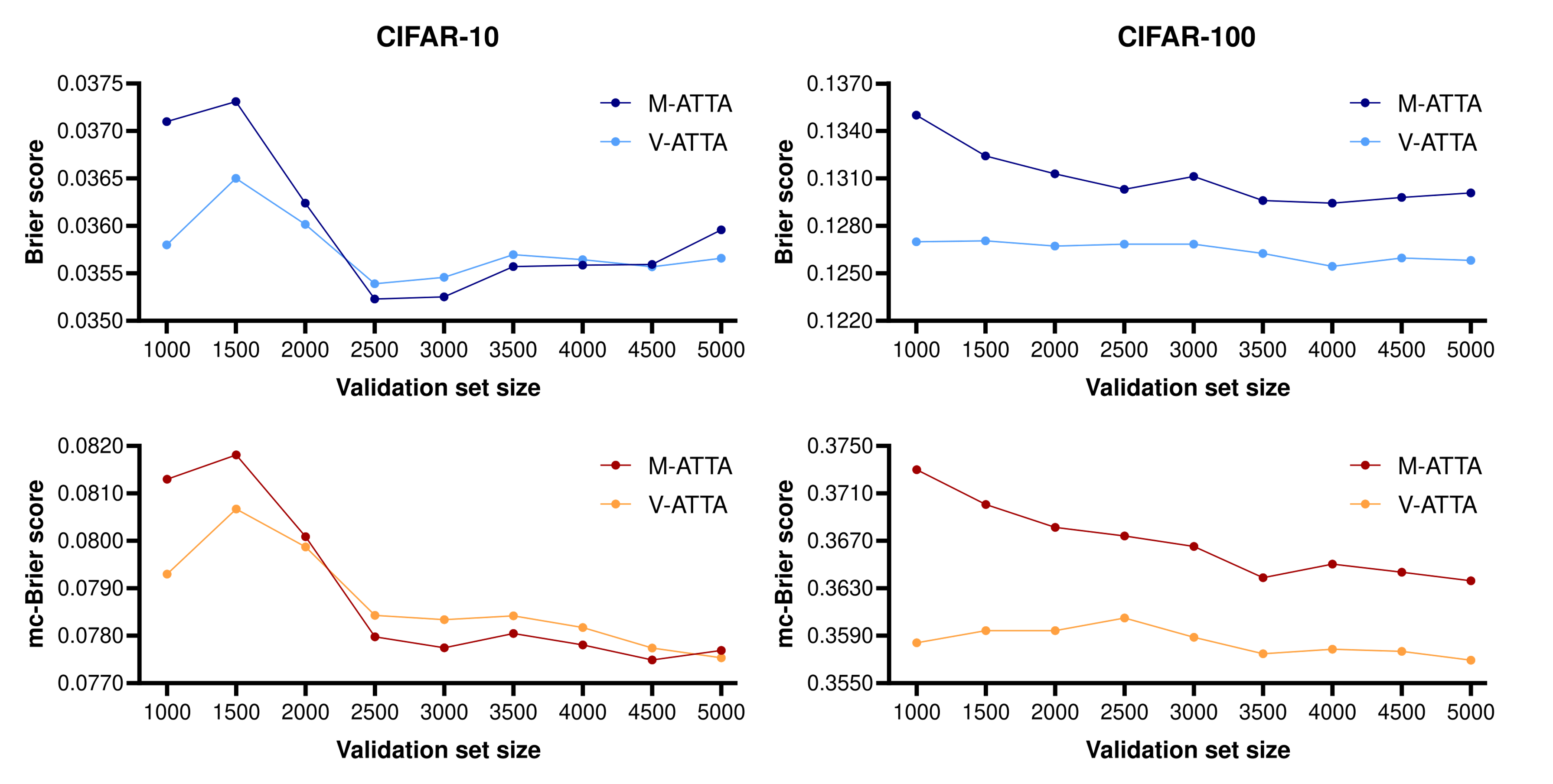
Figure 1: Comparing the Brier and mc-Brier scores obtained with M-ATTA and V-ATTA, with different validation/test set ratios, evaluated in the respective test sets of both CIFAR-10 and CIFAR-100 datasets.

All methods are evaluated with the described uncertainty calibration metrics - Brier score (both “classical” and multi-class version) and ECE (with 15 bins) - and also the widely known NLL loss. Although a proper scoring rule (and so, built to evaluate the quality of probabilistic predictions), the NLL loss (traditionally used in the training process of DNNs) cannot be considered a metric of calibration (or strong calibration) given our definition, because it only considers the quality of the predictions associated with the true class; nevertheless, given that it is a proper scoring rule and a popular metric, it is common to consider the NLL alongside to Brier score and ECE, when evaluating uncertainty calibration methods [20, 24, 13].
We start our analysis of the results in Table III by comparing all the uncertainty calibration methods against the vanilla approach. The first main observation derived in this context, is that our methods (M/V-ATTA) are the only that have consistently better performance than the vanilla approach, presenting better results in all evaluation metrics and all three datasets. Contrarily, temperature scaling worsens the performance in the AID dataset (Brier score, mc-Brier score), isotonic regression also worsens the performance in the AID dataset (Brier score) and histogram binning worsens the performance in CIFAR-10 (Brier score, mc-Brier score, NLL), CIFAR-100 (NLL) and AID (mc-Brier score, NLL) datasets.
Focusing now on highlighting the best results for each specific scenario, we observe that in all three datasets, one of our methods (M-ATTA or V-ATTA) is the best performing method in terms of Brier score, mc-Brier score and NLL. Focusing in the three aforementioned evaluation metrics: in both CIFAR-10 and CIFAR-100 datasets, V-ATTA is consistently the best performing method, while M-ATTA is consistently the second-best performing method; in the AID dataset, M-ATTA is consistently the best performing method, while V-ATTA is consistently the second-best performing method. On the other hand, when considering ECE, isotonic regression is the best performing method in the CIFAR-10 dataset, while histogram binning is best performing method in the remaining two datasets (these methods are actually biased to ECE evaluation, since they are binning-based methods, what can explain the particularly good behaviour with this metric); still in this context, M-ATTA is the second-best performing method in CIFAR-10, and V-ATTA is the second best performing method in CIFAR-100.
Some additional observations can be derived from Table III: histogram binning seems to be an unreliable uncertainty calibration method, given how it worsens multiple evaluation metrics in different datasets; the AID dataset is found to be an interesting case study, where all three post-hoc calibration baselines struggle to accomplish consistent results; the empirical evidence presented suggests that M-ATTA and V-ATTA are the most consistent and generally best performing methods.
Finally, while M-ATTA is always better - in terms of Brier score - in the validation sets (see Subsection 5.1), this is not observable when using the respective test sets. This behavior can suggest some type of over-fitting is happening in the optimization process of M-ATTA. It is not surprising that M-ATTA is more prone to over-fitting phenomena than V-ATTA, since it has a larger number of parameters (proportional to the number of classes in the respective dataset).

5.3 Validation size experiments

In the previous subsection we observed that, when considering Brier score, mc-Brier score and NLL, V-ATTA is the best performing method in CIFAR-10 and CIFAR-100 (that are datasets with similar characteristics) while M-ATTA is the best performing method in the AID dataset. While this is possibly justified by the different nature of the AID dataset (in comparison to CIFAR-10/100), we explore the possibility that the different behavior is caused by different proportions in terms validation/test sets. As such, this subsection is centered around experimenting with the ratio between the validation and the test set on the CIFAR-10 and CIFAR-100 datasets. With these experiments we also try to reduce the over-fitting phenomena in the M-ATTA method, since we are increasing the size of the validation sets.
The results are shown in Figure 1. In the presented experiments, both M-ATTA and V-ATTA are optimized with different validation/test set size ratios, beginning with 1000 validation set samples (like in Subsection 5.2) and iteratively adding 500 samples (while subtracting them from the test set) until reaching 5000 (this is done in both CIFAR-10 and CIFAR-100 datasets). In the CIFAR-10 dataset, we observe that M-ATTA actually outperforms V-ATTA when the validation set size is around the range between 2500 and 4000 (in this range the validation set size is approximately 1/3 of the test set size, just like in the AID setup for the previous experiments). On the other hand, in the CIFAR-100 experiments, although some improvement in performance is observed with M-ATTA, it is not enough to outperform V-ATTA. It is somewhat expected that the problem of over-fitting is easily addressed when working with CIFAR-10, since the M-ATTA model used in CIFAR-100 has ten times more parameters than the one used with CIFAR-10.

6 Final Remarks

Based on the results presented and discussed in the previous section, we highlight some conclusions derived from this work:

• The proposed methods (M-ATTA and V-ATTA) are the most robust, since - contrarily to the baseline methods selected for comparison - they never produce worse results (compared to the vanilla approach) with any of the selected evaluation metrics, and are always the best performing methods in terms of Brier score, mc-Brier score and NLL, independent of the dataset.

• Although generally the best performing, our methods lose to either isotonic regression or histogram binning when evaluated with the ECE. These baseline methods are somewhat biased towards ECE evaluation, since they leverage binning for obtaining better calibrated predictions; we speculate this justifies the inconsistency of these methods with the other evaluation metrics and the specially good performance with the ECE.

• V-ATTA is capable of outperforming M-ATTA with less parameters, in the CIFAR-10 and CIFAR-100 test sets, even though M-ATTA is always the best method in the respective validation sets. We speculate that M-ATTA is suffering of some over-fitting phenomena in these scenarios; in the case of CIFAR-10, we show this can be surpassed by increasing the size of the validation set (when considering Brier and mc-Brier scores).

For future work, we identify some challenges that can be addressed: studying different solutions for the partial over-fitting phenomena found with M-ATTA; exploring more complex types of augmentations; adapting our methods and extending their empirical evaluation to scenarios of object detection and/or semantic segmentation.

References

- [1] G. Blattenberger and F. Lad. Separating the brier score into calibration and refinement components: A graphical exposition. The American Statistician, 39(1):26–32, 1985.
- [2] G. W. Brier et al. Verification of forecasts expressed in terms of probability. Monthly weather review, 78(1):1–3, 1950.
- [3] P. Conde and C. Premebida. Adaptive-TTA: accuracy-consistent weighted test time augmentation method for the uncertainty calibration of deep learning classifiers. In 33rd British Machine Vision Conference 2022, BMVC 2022, London, UK, November 21-24, 2022. BMVA Press, 2022.
- [4] Y. Gal and Z. Ghahramani. Dropout as a bayesian approximation: Representing model uncertainty in deep learning. In international conference on machine learning, pages 1050–1059. PMLR, 2016.
- [5] T. Gneiting and A. E. Raftery. Strictly proper scoring rules, prediction, and estimation. Journal of the American statistical Association, 102(477):359–378, 2007.
- [6] A. Graves. Practical variational inference for neural networks. Advances in neural information processing systems, 24, 2011.
- [7] C. Guo, G. Pleiss, Y. Sun, and K. Q. Weinberger. On calibration of modern neural networks. In International Conference on Machine Learning (ICML), pages 1321–1330. PMLR, 2017.
- [8] C. Gupta and A. K. Ramdas. Top-label calibration and multiclass-to-binary reductions. arXiv preprint arXiv:2107.08353, 2021.
- [9] K. He, X. Zhang, S. Ren, and J. Sun. Deep residual learning for image recognition. In Proceedings of the IEEE Conference on Computer Vision and Pattern Recognition (CVPR), pages 770–778, 2016.
- [10] I. Kim, Y. Kim, and S. Kim. Learning loss for test-time augmentation. Advances in Neural Information Processing Systems (NeurIPS), 33:4163–4174, 2020.
- [11] A. Krizhevsky, G. Hinton, et al. Learning multiple layers of features from tiny images. 2009.
- [12] A. Lyzhov, Y. Molchanova, A. Ashukha, D. Molchanov, and D. Vetrov. Greedy policy search: A simple baseline for learnable test-time augmentation. In Conference on Uncertainty in Artificial Intelligence, pages 1308–1317. PMLR, 2020.
- [13] J. Moon, J. Kim, Y. Shin, and S. Hwang. Confidence-aware learning for deep neural networks. In International Conference on Machine Learning (ICML), pages 7034–7044. PMLR, 2020.
- [14] N. Moshkov, B. Mathe, A. Kertesz-Farkas, R. Hollandi, and P. Horvath. Test-time augmentation for deep learning-based cell segmentation on microscopy images. Scientific reports, 10(1):1–7, 2020.
- [15] R. Müller, S. Kornblith, and G. E. Hinton. When does label smoothing help? Advances in neural information processing systems, 32, 2019.
- [16] A. H. Murphy. A new vector partition of the probability score. Journal of Applied Meteorology and Climatology, 12(4):595–600, 1973.
- [17] M. P. Naeini, G. Cooper, and M. Hauskrecht. Obtaining well calibrated probabilities using bayesian binning. In Twenty-Ninth AAAI Conference on Artificial Intelligence, 2015.
- [18] A. Niculescu-Mizil and R. Caruana. Predicting good probabilities with supervised learning. In Proceedings of the 22nd International Conference on Machine Learning (ICML), pages 625–632, 2005.
- [19] J. Nixon, M. W. Dusenberry, L. Zhang, G. Jerfel, and D. Tran. Measuring calibration in deep learning. In CVPR Workshops, volume 2, 2019.
- [20] Y. Ovadia, E. Fertig, J. Ren, Z. Nado, D. Sculley, S. Nowozin, J. Dillon, B. Lakshminarayanan, and J. Snoek. Can you trust your model’s uncertainty? evaluating predictive uncertainty under dataset shift. Advances in Neural Information Processing Systems (NeurIPS), 32, 2019.
- [21] G. Pereyra, G. Tucker, J. Chorowski, Ł. Kaiser, and G. Hinton. Regularizing neural networks by penalizing confident output distributions. arXiv preprint arXiv:1701.06548, 2017.
- [22] J. Platt et al. Probabilistic outputs for support vector machines and comparisons to regularized likelihood methods. Advances in large margin classifiers, 10(3):61–74, 1999.
- [23] D. Shanmugam, D. Blalock, G. Balakrishnan, and J. Guttag. Better aggregation in test-time augmentation. In Proceedings of the IEEE/CVF International Conference on Computer Vision, pages 1214–1223, 2021.
- [24] J. Tian, D. Yung, Y.-C. Hsu, and Z. Kira. A geometric perspective towards neural calibration via sensitivity decomposition. Advances in Neural Information Processing Systems (NeurIPS), 34:26358–26369, 2021.
- [25] G. Wang, W. Li, M. Aertsen, J. Deprest, S. Ourselin, and T. Vercauteren. Test-time augmentation with uncertainty estimation for deep learning-based medical image segmentation. Medical Imaging with Deep Learning (MIDL), 2018.
- [26] G. Wang, W. Li, M. Aertsen, J. Deprest, S. Ourselin, and T. Vercauteren. Aleatoric uncertainty estimation with test-time augmentation for medical image segmentation with convolutional neural networks. Neurocomputing, 338:34–45, 2019.
- [27] D. Widmann, F. Lindsten, and D. Zachariah. Calibration tests in multi-class classification: A unifying framework. Advances in Neural Information Processing Systems (NeurIPS), 32, 2019.
- [28] G.-S. Xia, J. Hu, F. Hu, B. Shi, X. Bai, Y. Zhong, L. Zhang, and X. Lu. AID: A benchmark data set for performance evaluation of aerial scene classification. IEEE Transactions on Geoscience and Remote Sensing, 55(7):3965–3981, 2017.
- [29] B. Zadrozny and C. Elkan. Obtaining calibrated probability estimates from decision trees and Naive Bayesian classifiers. In International Conference on Machine Learning (ICML), volume 1, pages 609–616. Citeseer, 2001.
- [30] B. Zadrozny and C. Elkan. Transforming classifier scores into accurate multiclass probability estimates. In Proceedings of the eighth ACM SIGKDD international conference on Knowledge discovery and data mining, pages 694–699, 2002.