Comparison of modified black-body fits for the estimation of dust optical depths in interstellar clouds

Abstract

Context. When dust far-infrared spectral energy distributions (SEDs) are fitted with a single modified black body (MBB), the optical depths tend to be underestimated. This is caused by temperature variations, and fits with several temperature components could lead to smaller errors.

Aims. We want to quantify the performance of the standard model of a single MBB in comparison with some multi-component models. We are interested in both the accuracy and computational cost.

Methods. We examine some cloud models relevant for interstellar medium studies. Synthetic spectra are fitted with a single MBB, a sum of several MBBs, and a sum of fixed spectral templates, but keeping the dust opacity spectral index fixed.

Results. When observations are used at their native resolution, the beam convolution becomes part of the fitting procedure. This increases the computational cost, but the analysis of large maps is still feasible with direct optimisation or even with Markov chain Monte Carlo methods. Compared to the single MBB fits, multi-component models can show significantly smaller systematic errors, at the cost of more statistical noise. The $\chi^{2}$ values of the fits are not a good indicator of the accuracy of the $\tau$ estimates, due to the potentially dominant role of the model errors. The single-MBB model also remains a valid alternative if combined with empirical corrections to reduce its bias.

Conclusions. It is technically feasible to fit multi-component models to maps of millions of pixels. However, the SED model and the priors need to be selected carefully, and the model errors can only be estimated by comparing alternative models.

1 Introduction

Thermal dust emission at far-infrared and millimetre wavelengths is used to trace the structure and physical conditions of interstellar matter (ISM), especially in connection with star formation (SF). The targets range from a Galactic diffuse medium and local molecular clouds to entire galaxies. The measured intensities represent emission from a range of conditions that depends on both the nature of the sources and the angular resolution of the observations. The continuum emission also carries information about the dust itself, which is interesting due to the significant and systematic evolution that takes place in the dust properties during the SF process (Draine, 2003).

The long-wavelength dust emission is often modelled as modified black-body (MBB) emission, a black-body spectrum multiplied by a power law representing the frequency dependence of the dust absorption cross section $\kappa_{\nu}$. The analysis may assume both a single temperature $T$ and optically thin emission, which is only an approximation of the emission of any astronomical source. If the assumptions of a single temperature and optically thin emission are both violated, an analytical estimation of source properties is hardly possible, and more detailed modelling of the observations is needed. Even for optically thin sources, all observations consist of emission from dust at different temperatures within the telescope beam, both along the line of sight (LOS) and over the sky. The frequency dependence of $\kappa_{\nu}$ is also more complex than a single power law (Paradis et al., 2010; Planck Collaboration, 2014a, b; Gordon et al., 2014; Köhler et al., 2015; Juvela et al., 2015a). However, given the limitations as to the number of observed frequencies and the signal-to-noise ratio (S/N) of the data, the spectral energy distributions (SEDs) have to be modelled with just a few free parameters, which include at least the intensity and one temperature. The simultaneous fitting of temperature and $\beta$ is complicated by the inherent anti-correlation of these parameters, which makes the individual parameters very sensitive to noise (Shetty et al., 2009a; Kelly et al., 2012; Juvela & Ysard, 2012a; Juvela et al., 2013b). The problem is further complicated by temperature variations, which tend to systematically decrease the observed $\beta$ values relative to the actual $\beta$ of the dust (Shetty et al., 2009b; Juvela & Ysard, 2012b). If dust emission is only used to measure column densities, the results are likely to be more robust if $\beta$ is kept constant, even if the real variations of $\beta$ may then result in up to tens of percent errors in the column density estimates. Spectral indices can only be constrained with high-S/N data that cover a wide frequency range, and even then the estimates can still be biased due to the temperature variations.

The single-component MBB model can be extended by allowing multiple temperature or $\beta$ components. In studies of dust properties, one may further allow changes in $\beta$ as a function of frequency (Paradis et al., 2012; Gordon et al., 2014; Galliano, 2018). However, many sources are known to have wide temperature distributions, with smaller effects expected from the $\beta$ variations. Therefore, it is more common to use multiple temperature components while the dust optical properties are assumed to be constant or modelled with one free parameter at most. This is the case especially in studies of external galaxies, where most temperature structures remain unresolved (Galametz et al., 2012; Chang et al., 2021). However, temperature variations can be significant even in local SF clouds, from $\sim$6 K inside cold cores (Crapsi et al., 2007; Harju et al., 2008; Pagani et al., 2015) to more than 100 K in hot cores (Motte et al., 2018; Jørgensen et al., 2020). In Galactic studies, the single-component MBB model is still the main tool, although it suffers from the well-known tendency to underestimate column densities. The actual three-dimensional temperature fields can only be estimated with radiative transfer modelling or, in the case of geometrically simple objects, with tools such as the inverse Abel transform (Roy et al., 2014).

The calculation of multi-component MBB fits poses some technical challenges. The increased number of free parameters may require regularisation, for example by using parameter priors in the Bayesian framework. Especially the problem of $T-\beta$ correlations has led to the use of hierarchical models, where the hyper-parameters of the parameter distributions are fitted together with the parameters (i.e. $T$ and $\beta$) of individual measurements (Kelly et al., 2012; Galliano, 2018; Lamperti et al., 2019). The efficiency of priors and hierarchical models still varies from case to case. In a complex SF region, the priors must accommodate a wide range of temperatures and provide correspondingly weaker constraints for the individual measurements. There is also the risk of biasing the estimates for rare or unexpected sources, such as an individual hot (or cold) core seen against a field of colder (or warmer) background (Juvela et al., 2013b).

Marsh et al. (2015) have presented the point process mapping (PPMAP) method, which fits dust observations with a combination of fixed SED templates, such as MBB functions (Marsh et al., 2017; Howard et al., 2019, e.g.). The emission is represented by points in the state phase, and a requirement of using the minimum set of points to fit the data (to an accuracy of $\chi^{2}\sim 1$) also acts as regularisation. One important point is that PPMAP uses all observations at their native resolution. The more typical approach is to convolve all observations to a common lower resolution, which then allows the SED of each map pixel to be analysed independently. The use of the native data resolution brings additional challenges to the SED fitting. First, it requires higher S/N observations since the data are used at a higher resolution (more noise per resolution element) and the short-wavelength information of small-scale intensity variations is combined with weaker constraints on the SED shape, which partly depend on observations at longer wavelengths and lower angular resolutions. Second, the fitting can no longer be done pixel by pixel; it has become a global optimisation problem with a much higher computational cost.

In this paper, we use simulations of interstellar clouds to compare the precision of column density estimates calculated with the single-component MBB model and with some multi-component models. For the latter, we examine both the use of SED templates (here MBB functions with fixed temperatures) and the use of MBB functions with temperatures directly as free parameters. The observations are used at their original resolution by including the convolution with the telescope beam as part of the model. In view of the associated increased computational cost, we also pay attention to the organisation of calculations and the potential benefits of using graphics processing units (GPUs). The fits were mainly carried out with direct numerical optimisation, but some tests were also carried out using Markov chain Monte Carlo (MCMC) methods. The simulated observations include simple toy models with two temperature components and more complex cloud models where the synthetic observations were created through radiative transfer modelling.

The contents of the paper are the following. In Sect. 2 we present the multi-component MBB models and discuss some details of the SED fits. Section 3 presents the main results from the tests, which include toy models with ad hoc temperature distributions (Sect. 3.1), Bonnor-Ebert spheres with internal and external heating (Sect. 3.2), a cloud filament with stochastically heated grains (Sect. 3.3), and a large-scale cloud model based on magnetohydrodynamic (MHD) simulations (Sect. 3.4). We discuss the results in Sect. 4 before presenting the main conclusions in Sect. 5.

2 Methods

Dust emission can be approximated as MBB emission, where the observed intensity $I_{\nu}$ is

$$I_{\nu}=B_{\nu}(T,\beta)(1-e^{-\tau_{\nu}})\approx B_{\nu}(T)\tau_{\nu}=B_{\nu}(T)\Sigma\kappa_{\nu}(\nu_{0})\left(\frac{\nu}{\nu_{0}}\right)^{\beta},$$ (1)

where $T$ is in principle the dust temperature but more precisely the colour temperature that depends on all temperatures along the LOS. In Eq. (1) the optical depth $\tau$ is written as the product of mass surface density $\Sigma$ and the dust mass absorption coefficient $\kappa_{\nu}$, which is further assumed to follow a power law with the opacity spectral index $\beta$. The constant $\nu_{0}$ is an arbitrary reference frequency. In the following, Eq. (1), the modified black-body function, is written as $MBB(T,\beta)$.

When the emission originates from a source with a distribution of temperatures, the intensities may still be approximated with a sum of MBB function,

$$I_{\nu}\approx\sum_{i}W(T_{i})MBB(T_{i},\beta_{i}),$$ (2)

where the weights $W(T_{i})$ are the fitted parameters. We use two versions of Eq.( 2). In the $N$-MBB models, the fit is based on directly on the above equation at each map position $\bar{r}$,

$$I(\bar{r},{\nu})=\sum_{i}^{N}W_{i}(\bar{r})\,\,MBB_{\nu}(T_{i}(\bar{r}),\beta_{i}({\bar{r}})).$$ (3)

The model includes $N$ MBB functions, with $W_{i}(\bar{r})$ and $T_{i}(\bar{r})$ as the free parameters while the spectral index $\beta_{i}(\bar{r})$ is kept constant. With $N$=1, Eq.(3) describes the standard single-component MBB fit (1-MBB).

The alternative SED models $N$-TMPL correspond to

$$I_{\nu}=\sum_{i}^{N}W_{i}(\bar{r})\,\,C_{i}(\nu).$$ (4)

Here $C_{i}(\nu)$ are fixed spectral templates. These can be MBB functions for some fixed values of $T$ and $\beta$, the corresponding functions for some distributions of $T$ and $\beta$, or any other templates that could be expected to describe the observed emission. In the tests, we set $C_{i}(\nu)$ equal to MBB function at a given discrete temperature. Because the temperatures remain fixed during the fitting, the model is different from Eq. (3) and the scaling factors $W_{i}$ are the only free parameters of the $N$-TMPL models.

In Eqs.(3)-(4), the left side is the observed intensity $I_{\nu}$, which is the true sky surface brightness convolved with the telescope beam. In 1-MBB models, we follow the standard analysis, where all observations are convolved to a common lower angular resolution, the fit itself does not include convolutions, and each map pixel can be fitted completely independently. This analysis thus results in estimated intensity and temperature maps at the same common resolution. In all other cases, the model and the observations are compared at the original resolution of the observations. This means that the model predictions have to be convolved with the telescope beam on each step of fit. The resolution of the resulting column density maps is now not as well defined. The band with the highest resolution provides information of the sky brightness at that frequency and that resolution, while at least two bands are needed to trace temperature variations. The sensitivity to emission from dust at different temperatures varies between the bands, making the effective resolution of the resulting $\tau$ map less precise.

When convolution is part of the optimisation, the fit minimises the weighted least squares errors

$$\chi^{2}=\sum_{k}\left(\frac{I_{k}-M_{k}\otimes B_{k}}{\delta I_{k}}\right)^{2},$$ (5)

where $k$ refers to the frequency band, $M_{k}$ is the unconvolved model prediction (right-hand side of Eq.(3) or Eq.(4)), $B_{k}$ is the telescope beam, and ‘$\otimes$’ stands for convolution. The problem is computationally harder, since the model-predicted surface brightness maps are convolved with the telescope beams on every step of the optimisation and the fit parameters for the whole map are connected via the convolutions. The convolution can be done in real space, with direct summation over the beam footprint, or using Fourier transformation (fast Fourier transforms, FFTs). We use mainly the latter option, which is faster, but more limited in its ability to weight individual measurements or to handle missing values and map boundaries.

When beam convolutions are part of the fitting procedure, all parameters for the entire map are combined into a single optimisation problem. The large number of data points precludes the use second order information (i.e. Hessian matrices), which would lead to excessive memory usage. We use mainly conjugate gradient algorithms, where only the gradient of the $\chi^{2}$ function is needed (relative to each of the fitted parameters). The problem remains feasible, because the telescope beams couple data directly only over small distances. Therefore, although all fitted parameters are in principle connected, this connection is strong only over short distances.

If we denote the observed surface brightness values with $S$, the $\chi^{2}$ function of $N$-TMPL models becomes

$$\chi^{2}=\sum_{i,k}\left(\frac{S_{i,k}-[\sum_{c}W_{c}C_{c,k}\otimes B_{k}]_{i,k}}{\delta S_{i,k}}\right)^{2},$$ (6)

where the indices $i$, $k$, and $c$ refer to the position, the frequency band, and the SED template, respectively. Since the $T_{\rm C}$ values are pre-selected constants, the number of free parameters ($W_{c}$) is the same as the number of the fitted SED components.

For the $N$-MBB models the minimised function is

$$\chi^{2}=\sum_{i,k}\left(\frac{S_{i,k}-\left[\left(\sum_{c}M(I_{c},T_{c},\beta_{c}\right)\otimes B_{k}\right]_{i,k}}{\delta S_{i,k}}.\right)^{2}.$$ (7)

Here $M$ stands for the MBB function, and the term in square brackets denotes the convolved model-predicted map at one frequency. The index $i$ is omitted within the square brackets, but the result of the convolution is a function of position (index $i$) and frequency (index $k$). When $\beta$ is kept constant, the number of free parameters is two times the number of SED components. For better performance and to guarantee sufficient accuracy of the gradient estimates, it is important that the gradients are calculated analytically (Appendix A).

By default, the optimisation of $N$-TMPL models is performed in real space. However, the templates $C_{c,f}$ appear in Eq. 4 only as constant factors, and this makes it possible to move the optimisation to Fourier space. If the Fourier transformation is denoted by $\cal F$, one minimises

$$\chi^{2}=\sum_{i^{\prime},k}\frac{\left[{\cal F}(S_{i^{\prime},k})-\sum_{c}C_{c,k}{\cal F}(W_{i^{\prime},c})\right]_{i^{\prime},k}^{2}}{dS_{k}^{2}},$$ (8)

where the index $i^{\prime}$ now denotes an element in the Fourier space. The free parameters are the real and imaginary parts of the Fourier amplitudes that correspond to the real-space weight maps $W_{i,c}$. Because the elements ${\cal F}(W_{i^{\prime},c})$ result from the Fourier transformation of a real-valued function, only $n+(n-1)N$ non-redundant elements need to be optimised, where $N$ is the map size and $n=\lceil N/2\rceil$. Within the optimisation, the costly convolution is replaced with a direct multiplication. For the largest test cases, this amounts to a speedup of one or two orders of magnitude. If the observational noise in $S$ is Gaussian, the errors in the Fourier amplitudes are also normally distributed, justifying the use of the least-squares formula. One important restriction in Eq. (8) is that the error estimates $dS_{k}$ are now constant values for each frequency, not being able to be varied pixel by pixel. Compared to the alternative hypothesis of constant relative uncertainties over the maps, this leads to differences when a single beam contains widely different intensity values (changing locally the relative weight of the different pixels) or when the shape of the observed spectra changes significantly (changing locally the relative weighting of the different bands). It is also more difficult to implement general priors or even to constraint optical depths to positive values (i.e. to enforce $W_{i,k}\geq 0$). In the following, the fits performed in Fourier space are referred to as $N$-TMPL-F fits.

3 Results

We compared the performance of the SED models for different simulated observations. Results are presented for simple toy models (Sect. 3.1), a Bonnor-Ebert sphere, (Sect. 3.2), a filament that includes the emission from stochastically heated grains (Sect. 3.3), and finally for a more realistic large-scale magnetohydrodynamic (MHD) simulation (Sect. 3.4).

3.1 Toy models

3.1.1 Unconstrained fits

To get basic understanding of the performance of the $N$-TMPL and $N$-MBB models, we started with simple toy models. In Fig. 1a, the observations consist of two emission components, one at a $T_{1}$=15 K and another at a temperature that changes linearly over the 128$\times$128 pixel maps from $T_{2}$=10 K to $T_{2}$=20 K. The data include 160, 250, 350, and 500 $\mu$m maps with 3% relative observational noise. The beam size was set in all bands equal to half of the pixel size, to eliminate in this test the effect of the beam convolutions. This enables more direct comparison between the 1-MBB and multi-component models, when only the latter have the beam convolutions as part of the fitted model. The 2-TMPL model uses MBBs at $T=13$ K and $T=17$ K as the SED templates. The data were initially analysed assuming $\beta=1.9$, the same value that was used to generate the synthetic observations. Figure 1 plots the quantity $\tau/\tau_{0}$, the ratio between the estimated and the true optical depths.

The 1-MBB model behaves in Fig. 1a as expected. The correct optical depth $\tau$ is recovered when the emission consists of a single temperature ($T_{2}\sim T_{1}=15$ K), and $\tau$ is increasingly underestimated as the difference between the two temperature components increases. Since the model has only two free parameters, the scatter of the optical depth estimates is small.

The 2-TMPL model also has two free parameters ($W_{1}$ and $W_{2}$) and the $\tau$ scatter is similar to that of the 1-MBB model. However, the errors increase rapidly away from the two selected $T_{\rm C}$ values and are positive between the two $T_{\rm C}$ values and negative outside the $T_{\rm C}$ range.

The construction of the simulated data in Fig. 1a matches the assumptions of the 2-MBB model, which also provides practically unbiased results. However, the number of free parameters is four, and the statistical noise of the $\tau$ estimates is two times larger than in the 1-MBB and 2-TMPL cases. The absolute accuracy of the individual $\tau$ estimates is therefore on average not better than for the 1-MBB model.

Figure 1a quotes the $\chi^{2}$ values of the fits. In Fig. 1 and later, we always quote the $\chi^{2}$ values normalised by the number of fitted data points.

The values are not scaled with the degrees of freedom (which is not well defined for non-linear models or models containing constraints (Andrae, 2010)) and thus directly compares how well the models match the observed intensities. A smaller $\chi^{2}$ value (a good match to intensities) does not necessarily mean more accurate $\tau$ estimates. The 2-TMPL fit was done with MCMC calculations, and the plotted values are averages over the MCMC samples. We also plot the 1-$\sigma$ confidence region (containing 68% of the MCMC samples), which follows very closely the actual dispersion of the $\tau$ estimates. However, these do not reflect the true error, which is dominated by systematic errors.

Figure 1b uses a different set of synthetic observations. The optical depths are distributed in each pixel at different temperatures according to a Gaussian $N(T_{0},\sigma_{T})$. In the plot, $\sigma_{T}$ is 1 K for the first half of the x-axis and 5 K for the second half. The mean temperature $\left<T\right>$ increases in both halves linearly from 12 K to 20 K. The temperature distributions are also truncated to $T>8$ K. The 1-MBB model performs well, with 20% bias reached only at the lowest temperatures and with the wider $\sigma_{T}$5 K temperature distribution. Most 1-MBB estimates remain within the 1-$\sigma$ error band of the 2-MBB model that has larger statistical noise. Like in Fig. 1a, the systematic error of the 2-TMPL model are significant. This is true especially at the highest temperatures, where the dust temperature distribution extends clearly above the $T_{\rm C}$ values.

Figure 1c uses the same observations as frame b but the fits assume a lower value of $\beta=1.7$, which thus leads to lower $\tau$ estimates. The drop affects the 2-MBB fit slightly more than the 1-MBB fit, making the latter the most accurate in terms of the $\tau$ estimates. The wrong $\beta$ value also exacerbates the 2-TMPL errors at high temperatures, where the estimates now fall even below zero. The unphysical values are the result of the model trying to match the SEDs (with temperatures outside its $T_{\rm C}$ range) using a negative weight for the colder component and a larger positive weight for the warmer component. It is thus clear than the over 10 K range of dust temperatures cannot be satisfactorily fitted with just two $T_{\rm C}$ components.

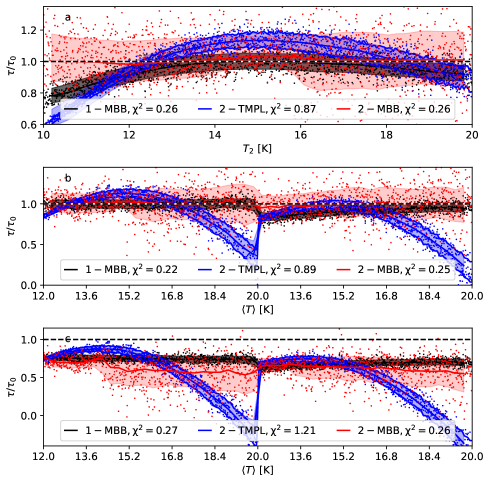
Figure 1: Ratio of estimated and true optical depths $\tau/\tau_{0}$ for 1-MBB, 2-TMPL ($T_{\rm C}$=13 K and 17 K), and 2-MBB models. The observations consist of 160, 250, 350, and 500 $\mu$m intensities with 3% relative noise. The dots correspond to individual pixels (every 10th pixel), the solid lines show moving averages, and the shaded regions the 1-$\sigma$ dispersion of the $\tau$ estimates. The $\chi^{2}$ values of the ML fits (normalised by the number of fitted data points) are quoted in the frames. In frame a, observations consist of one emission component at $T_{1}=15$ K and one component varied in the range $T_{2}$=10-20 K (on x-axis), both with the same optical depth. The additional solid blue lines correspond to the 1-$\sigma$ error estimates from the MCMC fit of the 2-TMPL model. In frame b, the observations correspond to a continuous temperature distribution, $T\sim N(\langle T\rangle,\sigma_{T})$. The x-axis shows the $\langle T\rangle$ value, with $\sigma_{T}=1$ K for the first and $\sigma_{T}=5$ K for the second half. Frame c is the same as frame b but the SED fits assuming $\beta=1.7$ instead of the correct value of $\beta=1.9$.

3.1.2 Fits constrained with priors

Figure 2 shows the corresponding results, where we include a prior $T\sim N(18\,{\rm K},\/5\,{\rm K})$ for the 2-MBB fits. The intensities of the 2-MBB fits (parameters $I_{i,c}$) and the 2-TMPL fits (parameters $W_{i,c}$) are restricted to non-negative values by optimising the logarithm of the relevant variables (cf. Appendix A). With these constraints, both models could be successfully fitted using MCMC. There is little difference between the 1-MBB and 2-MBB fits, although the latter has a smaller bias in the case of the $\sigma(T)=5$ K observations. The non-negativity has a clear effect on the 2-TMPL fits, as the optical depths are now overestimated rather than underestimated for temperatures above the $T_{\rm C}$ range. This shows that the Fig. 1b fit already contained negative components, even when the total $\tau$ estimates were positive. Although the unphysical negative values have been eliminated, the $\chi^{2}$ values of the fits are now much larger and the systematic errors of the $\tau$ values still increase rapidly outside the adopted $T_{\rm C}$ range.

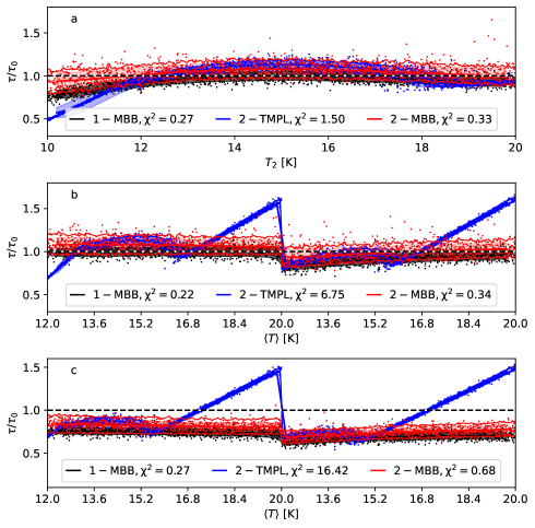
Figure 2: Same as Fig. 1, but forcing each component of the 2-MBB and 2-TMPL models to positive optical depths. In the case of 2-MBB, the model also includes a prior on the temperatures, $T\sim N(18\,{\rm K},\/\/5\,{\rm K})$. The plotted 2-TMPL and 2-MBB data are from MCMC calculations while the $\chi^{2}$ values are the average values of the maximum-likelihood solutions.

Figure 3 shows fits for 3-TMPL and 3-MBB models. With $T_{\rm C}=$13, 15.5, and 19 K, the bias in 3-TMPL results can be constrained to $\sim$20%. With a prior of $T\sim N(15\,{\rm K},\/3\,{\rm K}$, the results of 3-MBB fits are unbiased in the $\sigma_{\rm T}=1\,{\rm K}$ part of the map (left half of the plot) but still underestimate the $\sigma(T)=5$ K observations by $\sim$10%. Even if the systematic errors are partly smaller than in the 1-MBB fit, there is no clear net improvement because of the larger statistical noise.

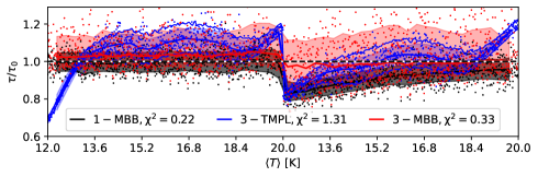
Figure 3: Same as Fig. 2b, but including results for 3-TMPL (MCMC fit) and 3-MBB (ML fit) models. The 3-TMPL model uses $T_{\rm C}=$13, 15.5, and 19 K, and the 3-MBB model includes a temperature prior $T\sim N(15\,{\rm K},\/\/3\,{\rm K})$.

3.1.3 Fits including beam convolution

Figure 4 shows the first comparison where the beam size is different for different bands. The synthetic observations correspond to the sum of two temperature components. The first one is at 15 K, apart from two Gaussian sources where the temperature changes to 10 K or 20 K. The second temperature component increases linearly from 10 K to 20 K over the map. The pixel size is 10$\arcsec$, and the full width at half maximum (FWHM) values of the Gaussian beams 20, 20, 25, and 36$\arcsec$ at 160, 250, 350, and 500 $\mu$m, respectively. The observations contain 3% relative noise at the resolution of the each map, and all results correspond to the ML solutions.

In Fig. 4, the 1-MBB model has again the lowest statistical errors, partly because all data have been convolved to a $36\arcsec$ resolution. The systematic errors exceed 20% when the 15 K component is combined with the extended second component at $\sim$10 K. (leftmost part of Fig. 4c), when the warm Gaussian source is combined with cold extended emission (around pixels index $\sim$4500), and even more significantly when the warm 17-18 K extended emission is combined with the cold Gaussian source (pixel indices $\sim$12000).

The 2-TMPL model uses values $T_{\rm C}$=13 K and 18 K. The statistical noise is larger than for the 1-MBB model but now also corresponds to a factor of two higher angular resolution. The angular resolution of the model is nominally $20\arcsec$, but because it uses all bands up to the 500 $\mu$m map with 36$\arcsec$ resolution, the solution might exhibit weak correlations up to that scale. The $\tau$ values are again significantly underestimated, when the emission contains emission from dust below the $T_{\rm C}$ values. At the location of the cold Gaussian source (10 K against the $\sim$17-18 K background), the bias reaches 50%, the same as for the 1-MBB model. Towards the map centre, the emission corresponds to the single 15 K temperature and $\tau$ is overestimated by up to 20%.

The results of the 2-MBB model are practically unbiased. However, apart from the effect of convolutions, the synthetic observations also precisely match the assumptions of the 2-MBB model. The dispersion of the $\tau$ estimates is larger than for the other SED models and also larger than in the previous examples. Thus, the overall accuracy is only slightly better than for the 1-MBB model, which however also corresponds to a lower resolution. When the convolutions were performed using FFTs, the fits took of the order of one minute for the 128$\times$128 pixel maps.

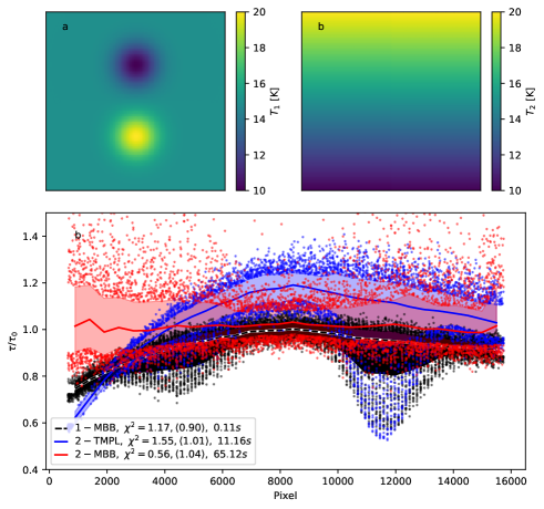
Figure 4: SED fits considering the effect of telescope beams. The 2-TMPL and 2-MBB cases include beam convolution as part of the fit while the 1-MBB fit is done at the lowest common resolution. The dust emission consists of the two temperature components shown in frames a and b. The map size is 128$\times$128 pixels, the pixel size 10$\arcsec$, and FWHM beam sizes 20$\arcsec$, 20$\arcsec$, 25$\arcsec$, and 36$\arcsec$ at 160, 250, 350, and 500 $\mu$m, respectively.

3.2 Bonnor-Ebert sphere

We calculated synthetic surface brightness maps for a 2.6 $M_{\sun}$ critically stable Bonnor-Ebert (BE) sphere (Ebert, 1955; Bonnor, 1956), with an assumed gas temperature of 15 K. However, in the subsequent radiative transfer modelling the cloud is illuminated from the outside, with the Mathis et al. (1983) interstellar radiation field (ISRF), and optionally from the inside by a $10\,L_{\sun}$ point source that is modelled as a 10000 K black body. These result in continuous radial dust temperature gradients and each LOS has emission from a different range of temperatures. In the outer parts, the colour temperature approaches 18 K. In the inner parts, the temperature is below 14 K for the externally heated and over 30 K for the internally heated case. The pixel size is set to 6$\arcsec$, with beam sizes 18$\arcsec$, 18$\arcsec$, 25$\arcsec$, and 36$\arcsec$ at 160, 250, 350, and 500 $\mu$m, respectively. The subsequent SED fits assume a constant $\beta$, which corresponds to the 160-500 $\mu$m spectral index of the dust model used in the radiative transfer calculations (Compiègne et al., 2011).

Figure 5 shows results for the externally heated model. The 1-MBB model provides even surprisingly accurate results (at 36$\arcsec$ resolution). The 2-TMPL model uses $T_{\rm C}$ values of 14.5 K and 17 K. These provide accurate estimates towards the cloud centre but overestimate $\tau$ in the outer parts, where the dust temperatures are above the $T_{\rm C}$ values. The 3-TMPL model has $T_{\rm C}$ values of 14, 15, and 17 K. Because the highest $T_{\rm C}$ is the same as in the 2-TMPL fit, the results are similar in the outer parts of the cloud, but there is minor improvement at the centre (corresponding to the added $T_{\rm C}$ value). The width of the LOS temperature distribution appears to be sufficiently narrow so that the 1-MBB model, by adapting to the LOS mean temperature, still performs well compared to the 3-TMPL model. The 2-TMPL and 3-TMPL fits enforced the positivity of the component weights but used no other priors. Without the positivity requirement, the $\chi^{2}$ values would be lower but especially the 2-TMPL result would include negative weights at some radial distances.

The 2-MBB fits in Fig. 5 were also calculated without priors. The estimates are mostly unbiased but show a relatively high scatter. The corresponding noise in the temperature being visible in Fig. 5d-e, where temperatures are not well constrained for individual pixels, at scales below the beam size. The low $\chi^{2}$ value also indicates the possibility of some overfitting.

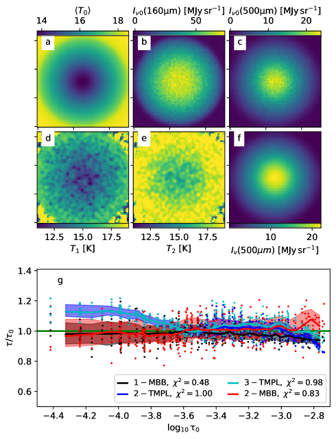
Figure 5: Fits on synthetic observations of an externally heated Bonnor-Ebert sphere. Frames a-c show the mass-weighted average LOS temperature of the model cloud and the calculated 160 $\mu$m and 500 $\mu$m surface brightness maps. Frames d-e show the temperature maps and frame f shows the 500 $\mu$m predictions from the 2-MBB model. Frame g shows the ratio of the estimated and true optical depth ($\tau/\tau_{0}$) as the function of $\tau_{0}$ for the four cases listed in the legend. The solid lines are moving averages, the shaded regions indicate the 1-$\sigma$ interval in the $\tau/\tau_{0}$ values, and the individual pixels outside this interval are shown as dots.

Figure 6 shows the corresponding results for the internally heated BE model. The errors of the 1-MBB fit increase to 20% towards the cloud centre. The selected $T_{\rm C}$ values are 18 and 25 K for the 2-TMPL model and 18, 23, and 29 K for the 3-TMPL model. The 2-TMPL model is unable to follow the rapid temperature changes in the centre, and the oscillating errors result in some artefacts in the estimated radial density profiles. The 3-TMPL model performs better at the very centre, but the overall accuracy is not much better than for the 1-MBB model.

The 2-MBB model shows increasing bias towards the cloud centre and the $\tau/\tau_{0}$ curve actually follows that of the 1-MBB model predictions. This is partly a coincidence, because the latter correspond to a factor of two lower angular resolution. At the centre of the projected cloud, the 2-MBB fit uses two temperatures that are both close to 30 K and separated from each other by some 4 K. This is still quite small compared to the full range of the actual LOS temperatures, which extend from $\sim 17$ K to over 50 K, (the highest temperatures at scales below the beam sizes).

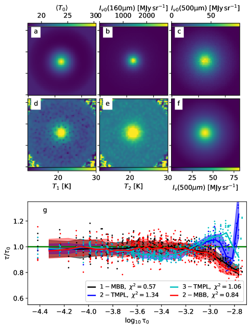
Figure 6: Same as Fig. 5, but for a BE sphere with an additional internal radiation source. The $T_{\rm C}$ values of the 2-TMPL and 3-TMPL models are given in the text. The resolution is 36$\arcsec$ for the 1-MBB model and 18$\arcsec$ for the other fits (for a nominal pixel size of 6$\arcsec$).

3.3 Filament with stochastically heated grains

We examined the optical depth estimates also as a function of the wavelengths. This has already been studied extensively from the point of view of observational noise and the LOS temperature variations (Shetty et al., 2009b, a; Malinen et al., 2011; Juvela & Ysard, 2012a, b; Juvela et al., 2013a, b). Below the main questions are related not only to the relative performance of the $N$-MBB and $N$-TMPL methods but also to the potential effect of stochastically heated grains.

We used the filament simulations of Juvela & Mannfors (2022). The model is discretised onto a Cartesian grid of 200³ cells with a cell size of 0.0116 pc. The model consists of a single filament with a Plummer-like column density profile

$$N=N_{0}[1+(r/R_{0})^{2}]^{(1-p)/2}$$ (9)

with $R_{0}$=0.0696 pc and $p$=3. The column density perpendicular to the filament major axis is set to $N({\rm H}_{2})=10^{22}$ cm^-2. The filament is illuminated by a normal ISRF (Mathis et al., 1983). There can be an additional 15 700 K point source with a 590 $\rm L_{\sun}$ luminosity, which is is placed 0.93 pc in front of or to one side of the filament. The source is 0.93 pc from the map centre, in a direction parallel to the filament main axis. The dust properties, including those of stochastically heated grains, are taken from Compiègne et al. (2011).

We calculated 200$\times$200 pixel maps, where the pixel size corresponds to the 3D discretisation and is set equal to 5$\arcsec$ (corresponding to a distance of 479 pc). Synthetic surface brightness maps were computed at 70, 100, 160, 250, 350, and 500 $\mu$m with the assumed angular resolutions of 10$\arcsec$, 10$\arcsec$, 12$\arcsec$, 18$\arcsec$, 25$\arcsec$, and 36$\arcsec$, respectively. The wavelengths and resolutions are similar as in Herschel observations, except for the lower angular resolutions adopted for the 70 and 100 $\mu$m bands.

In the absence of the point source, the 1-MBB fits of the 160-500 $\mu$m observations give a narrow range of colour temperatures from 16 K to 17.7 K. Based on this, we selected temperatures $T_{\rm C}$=16 K and 17 K for the 2-TMPL and $T_{\rm C}=$14, 16, and 18 K for a 3-TMPL fit. When the point source is added on the LOS towards the filament (0.93 pc in front of the filament and 0.93 pc from the projected map centre), the range of 1-MBB colour temperatures becomes 19.5-26 K. If the point source is to one side of the filament, the maximum exceeds 40 K but only towards the source position, in a region of relatively low column density. In these cases, we used $T_{\rm C}$=21 and 25 K for the 2-TMPL fits and $T_{\rm C}$=20, 23, and 26 K for the 3-TMPL fits. All surface-brightness observations contain 3% relative noise.

Figure 7a shows SEDs towards the map centre. These correspond to a single pixel and models without the point source or with the point source on the LOS towards the filament centre (but offset from the 3D centre of the filament). The fits show the systematic increase of the colour temperatures as the 1-MBB fits are extended to higher frequencies. The lower frame shows how the SED fits translate to $\tau$ estimates. The optical depths tend to be underestimated, and this also applies to the 2-TMPL and 3-TMPL models. The systematic error is largest for the 1-MBB model, roughly equal for the 2-TMPL and 3-TMPL models, and smallest for the 3-TMPL model. Like the average colour temperature, the bias of the $\tau$ estimates tends to increase as shorter wavelengths are included in the fit. The exception are the 2-MBB fits, where the statistical errors dominate. The error bars in Fig. 7b correspond to the $\tau$ estimates over a 0.7 pc long section of the filament spine. In models containing a point source, this section also includes the projected location of the point source.

Figure 7b shows that the $\chi^{2}$ values per data point of the 2-MBB fits are of the order of one for all band combinations. In the 1-MBB fits, the increase in the number of bands is associated with a rapid increase of $\chi^{2}$ values (as indicated by the SEDs in frame a). A similar trend exists for the 2-TMPL model and to a lesser extent for the 3-TMPL model, these of course depending on the chosen $T_{\rm C}$ values.

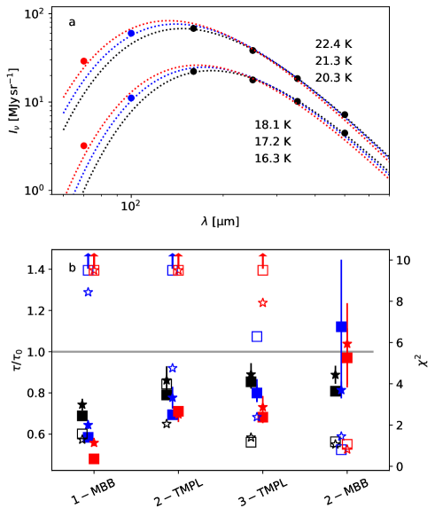
Figure 7: SED fits of the filament models. Frame a shows the SEDs towards the map centre and the 1-MBB fits to the 4-6 longest wavelength bands. The lower set of symbols and curves corresponds to a model without a point source, and the upper ones to a model with a point source on the LOS towards the filament but at 0.93 pc in front of the filament. The colour temperatures of the 1-MBB fits are quoted in the frame. Frame b shows the ratio of recovered and true peak optical depths (left axis, filled symbols) and the average $\chi^{2}$ per data point over the whole map (right axis, open symbols). The x-axis indicates the four models. The square and star symbols are, respectively, for the externally heated model and the model with a point source. The black, blue, and red symbols correspond to fits that extend to shortest wavelengths of 160, 100, and 70 $\mu$m, respectively. The error bars show the standard deviation of the optical depth estimates along the filament spine.

3.4 MHD cloud simulation

As the final test we examined a MHD cloud simulation. The full model volume is (4 pc)³ in size, but we used only the subvolume of (1.84 pc)³ that contains the densest structures. The column densities reach values above $N({\rm H}_{2})\sim 10^{23}$ cm^-2, while the average volume density is still below 10³ cm^-3. The simulation includes a few hundred embedded sources that increase the temperature variations. Details of the MHD simulation can be found in Haugbølle et al. (2018) and of the radiative transfer modelling in Juvela et al. (2022). Because the model includes a filamentary structure reminiscent of a small infrared dark cloud (IRDC), we refer to the model as the IRDC cloud.

The synthetic observations consist of maps at 160  250  350, and 500 $\mu$m. The effect of stochastically heated grains is not included. For the SED fitting, the main challenges are the large map sizes and the temperature variations associated with the cores. The 3D dust temperatures vary from less than 10 K in the cold cores to up to $\sim$100 K in the hot cores, but the range of the observed colour temperatures is naturally smaller. The surface brightness maps have 1875$\times$1875 pixels, and the assumed beam sizes are 2.3 , 2.3, 3.1, and 4.5 pixels at 160  250  350, and 500 $\mu$m, respectively. We use the same wavelengths as in previous tests, although the above scaling would correspond to a source distance of only 25 pc for a telescope of the Herschel size. The observational noise is 3% of the observations.

Below we compare the 1-MBB results to 3-TMPL and 3-MBB fits and then, with additional priors, to $N$-TMPL and $N$-MBB fits with $N>3$. We also look at the $N$-TMPL fits made in Fourier space separately, because those adopt a different noise model and are more limited in the use of priors. We are also interested in the relative run times.

3.4.1 IRDC cloud and 2-MBB and 4-TMPL fits

Figure 8 compares the 1-MBB fit to the results from 2-MBB and 4-TMPL fits for a 256$\times$256 pixel area of the full IRDC maps. Even this small region includes more than two orders of magnitude differences in surface brightness, with colour temperatures ranging from $\sim$14 K to over 30 K. The analysis uses a $\beta$ value that is correct for the 160-500 $\mu$m interval. The 4-TMPL fit uses $T_{\rm C}$ values of 15, 18, 22, and 27 K. The models were fitted without direct priors, except for the temperatures of the 2-MBB fit being limited to values above 8 K.

In the 1-MBB fits, the average ratio between the estimated and true optical depths is $\langle\tau/\tau_{0}\rangle=0.81$ and the standard deviation $\sigma(\tau/\tau_{0})=15$%. The optical depths are always underestimated, and the errors reach $\sim$60% in a region that contains the superposition of warm extended emission and a more compact and colder filamentary structure. The $\chi^{2}$ values are mostly well above one and in this case also correlated with the magnitude of the systematic $\tau$ errors.

For the 2-MBB and 4-TMPL fits, the morphology of the $\tau$ and $\chi^{2}$ maps is similar to the 1-MBB case. The bias of the $tau$ estimates is somewhat lower, and also the $\chi^{2}$ values are lower, especially considering that they refer to up to a factor of two higher angular resolution. The maximum errors are still almost $50$% but they are limited to smaller regions. The $T_{\rm C}$ values of the 4-TMPL model were chosen so that they result in accurate $\tau$ estimates. However, the results are not very sensitive to the precise $T_{\rm C}$ values, as long as they cover the range of colour temperatures in the 1-MBB fit.

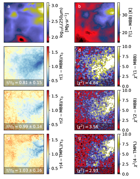
Figure 8: IRDC observations fitted with 1-MBB, 2-MBB, and 4-TMPL models. Frames a-b show the 250 $\mu$m intensities and colour temperatures from the 1-MBB fit. The second row shows the 1-MBB $\tau$ estimates relative to the correct values (frame c) and the $\chi^{2}$ values (frame d). The third and fourth rows show the corresponding data for the 2-MBB and 4-TMPL fits. The plots cover a 256$\times$256 pixel area of the IRDC cloud model.

3.4.2 IRDC cloud and 11-TMPL and 4-MBB fits

When $N$ is increased further, the $N$-TMPL and $N$-MBB fits require additional constraints. When $\beta$ is kept constant, a 4-MBB model has eight free parameters and an 11-TMPL model has 11 free parameters, both thus much larger than the number of the observed wavelengths.

Figure 9 shows results for the same area as in Fig. 8. The $T_{\rm C}$ values of the 11-TMPL model are placed logarithmically between 12 K to 40 K. The temperature prior is $T\sim N(25\,{\rm K},3\,{\rm K})$ for both the 4-MBB and 11-TMPL fits. The large $\chi^{2}$ values in the upper right hand part show that the fits do not yet correctly describe the complex temperature distributions of this area. Elsewhere in the maps the $\chi^{2}$ values are at or below $\sim 1$, but low $\chi^{2}$ values do not translate to more accurate $\tau$ estimates. The $\tau/\tau_{0}$ ratios are now more constant but there is also higher positive bias. The use of different apparently reasonable priors result in $\langle\tau/\tau_{0}\rangle$ varying by more than 10%. In particular, weaker priors tend to lead to larger temperature fluctuations and larger positive bias in $\tau$. In all cases, the dispersion in the $\tau/\tau_{0}$ ratios is equal or larger than in the 1-MBB case (not accounting for the difference in the angular resolutions).

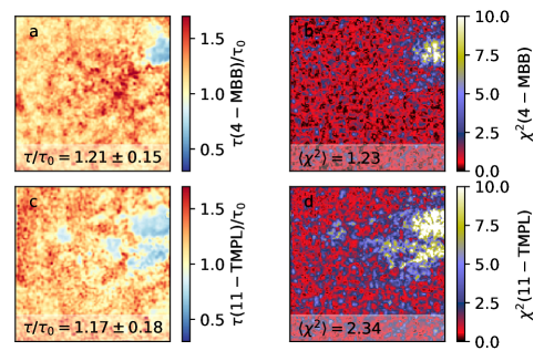
Figure 9: Fits of IRDC model maps with 4-MBB and 11-TMPL models. The corresponding data for the 1-MBB fit are shown in Fig. 8.

The same fits for the whole 1875$\times$1875 pixel maps are shown in Appendix B. The average statistics are similar to the previous image, although the lower average column density results in lower average bias, especially in the case of the 1-MBB fit. However, there are also regions of stronger internal heating, where all the fitted SED models can underestimate the optical depths by up to 60%.

3.4.3 IRDC cloud and $N$-TMPL fits in Fourier space

Fits of the $N$-TMPL model in Fourier space (i.e. $N$-TMPL-F fits) are attractive because of the faster computation, even if it only allows limited use of priors. The error estimates are also required to be constant over the map, and we set them equal to the mean of the 3% relative uncertainties. We also add to the minimised $\chi^{2}$ function a penalty

$$P=\xi\sum_{i}W_{i}^{2}.$$ (10)

This biases the solution against individual high $W_{i}$ and, more importantly, makes it unlikely that an observation would be fitted as a sum of positive and negative terms instead of a smaller number of smaller positive components.

Figure 10 compares the 1-MBB results to the 4-TMPL-F and 12-TMPL-F fits. The $T_{\rm C}$ values were placed logarithmically in the range 11-45 K. The fits were done without direct priors on the temperature. However, the 12-TMPL-F fit included a small penalty according to Eq. (10), with a $\xi$ values such that the effect on the final $\chi^{2}$ was $\la 1$%.

The 1-MBB results are identical to the previous tests, apart from the difference in the adopted error estimates, and still underestimate the true optical depth by up to 60%. Although the differences are not very large, the 4-TMPL and 12-TMPL fits are here more accurate, with a more symmetric error distribution around the correct value. The average $\langle\tau/\tau_{0}\rangle$ value of the 12-TMPL-F fit varies by $\pm 0.1$ units if the number of components is changed between 10 and 20, the lower limit of the $T_{\rm C}$ values between 10 K and 14 K, and the upper limit between 30 K and 40 K. The 4-TMPL-F fit is also relatively robust with respect to selected $T_{\rm C}$ grid. The 10% and 90% percentiles of the $\tau/\tau_{0}$ ratios (shown in Fig. 10) are very similar for the 4-TMPL and 12-TMPL fits, in spite of the factor of two difference in the $\chi^{2}$ values.

The upper right corner includes a region where the 4-TMPL-F and 12-TMPL-F fits overestimate $\tau$ by almost $\sim$60%. If the $T_{\rm C}$ grid is extended to 55 K, the maximum errors of the 12-TMPL-F fit are confined to a more symmetric range of [-35%, +31%]. This is in agreement with the maximum LOS temperatures being higher than the maximum 1-MBB colour temperatures of $\sim$35 K. When the highest $T_{\rm C}$ is 35 K, some components around $T_{\rm C}\sim 30$ K have negative weights in the area of the largest $\tau$ errors, in spite of the use of Eq. (10) penalty. The solution is thus partly unphysical, although, to the extent that the emission is in the Rayleigh-Jeans regime, this does not translate to large errors in the $\tau$ estimates. When the $T_{\rm C}$ grid is extended to higher temperatures, practically all weights remain positive.

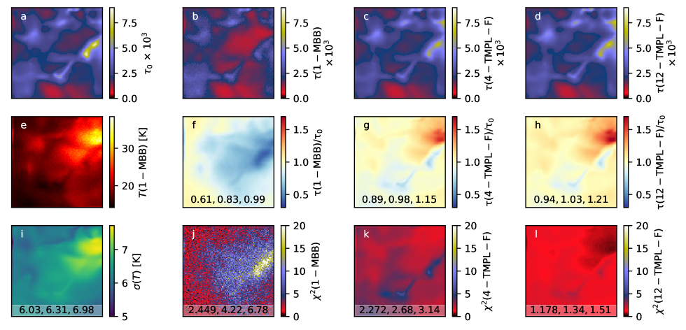
Figure 10: IRDC observations fitted in Fourier space. Frame a shows the true optical depth and frame e the colour temperature from the 1-MBB fit. Frames b-d show the optical depths estimated with the 1-MBB, 4-TMPL, and 12-TMPL fits, respectively. The corresponding ratios of estimated and true optical depths are shown in frames f-h and the $\chi^{2}$ values in frames j-l. Frame i shows the standard deviation of the temperature values from the 12-TMPL fit. The values quoted in the frames are the 10%, 50%, and 90% percentiles of the plotted quantity. The maps cover the same 256$\times$256 pixel area as in Fig. 8.

The fits performed with the same parameters for the whole 1875$\times$1875 pixel maps are shown in Appendix B. Due to the lower average column density, the mean bias of the 1-MBB estimates is there closer to zero (Fig. 20), and also the 10-90% intervals of the $\tau/tau_{0}$ ratios are similar between the fits. There is a number of hot sources where $\tau$ is underestimated by all three methods.

4 Discussion

Most studies model the FIR dust emission with a single MBB function (1-MBB), and the observations (the noise level and number of observed wavelengths) also may not allow much more complex analysis. The main problem of the single-temperature model is the underestimation of column densities (Shetty et al., 2009b; Juvela & Ysard, 2012b). The bias depends on the width of the temperature distribution, which makes SF regions with hot and cold cores particularly challenging. We have examined in this paper the use of multi-component SED models, using observations at their native resolution. We discuss the main findings below.

4.1 Basic tests

When the number of free parameters is less than the number of observed wavelengths, the SED fits can be done without additional constraints. The use of prior distributions may still be beneficial, especially when the data have low S/N.

In the tests of Sect. 3.1 and Sect. 3.2, the 2-MBB fits provided only small improvement over the 1-MBB fit. They resulted in lower bias in the $\tau$ estimates but with a larger statistical noise. The $\chi^{2}$ values were not directly correlated with the precision of the $\tau$ estimates. The low number of SED components was more of a problem for the 2-TMPL model, because the $T_{\rm C}$ values remain fixed and, unlike in the $N$-MBB models, not adjusted for each LOS separately. The errors depended on the distance between the $T_{\rm C}$ values and the actual source temperatures and increased rapidly outside the $T_{\rm C}$ range. This is a problem, since the full range of temperatures may not be known a priori and is difficult to estimate from observations. On the other hand, the errors may have been exaggerated in Sect. 3.1, because of the discrete temperature values of the synthetic observations. In real sources the temperature distribution is always wider, leading to less sharp changes in the bias.

In Sect 3.2, the internally heated Bonnor-Ebert sphere could not be fitted properly with just two temperature components. The absolute errors of the 3-TMPL were below $\sim$20% but showed rapid oscillations as the mean LOS temperature moved across the $T_{\rm C}$ grid. When the true solution is not available, such oscillation cannot be recognised, and this could have a significant effect on the derived density profiles. When beam convolutions are included in the SED models, the 2-MBB model also showed some problems with temperature oscillations at scales below the beam size. When the predictions of such a model are convolved to the observed resolution, the SED fits may be perfect but the predicted column densities will show positive bias that depends especially on pixels with the coldest temperatures. This might require additional constraints on the smoothness of the solution, provided that temperature field in the source is indeed assumed to be smooth at the observed resolution. Such priors would also affect the effective angular resolution of the obtained $\tau$ maps.

4.2 Filament with stochastically heated grains

In Sect. 3.3, we examined the dependence of $\tau$ estimates on the observed wavelengths in the 70-500 $\mu$m range. It is well known that the inclusion of shorter wavelengths tends to increase the estimated temperatures (e.g. Shetty et al., 2009b). This is based on the warmer dust having a higher contribution (relative to its mass) to the observed intensities. We had additional effects from stochastically heated grains that contributed significantly only to the shortest wavelengths. In a strong radiation field, the 70 $\mu$m emission could be emitted by warm large grains, but in our model the stochastically heated grains dominated the 70 $\mu$m observations and had a clear contribution to the 100 $\mu$m emission.

When the fitted wavelength range was extended from 160-500 $\mu$m to 70-500 $\mu$m, the optical depths were increasingly underestimated. The error was always more than 20% in the 1-MBB fits and mostly around 20% for the other fits. The 2-MBB fit was an exception, showing no clear bias (partly because of the larger statistical errors). There was no large difference between filaments that were illuminated by an isotropic radiation field or also by a nearby star. The main effect is that a higher radiation field results in higher temperatures, which always tends to decrease the systematic errors by moving the observations further into the Rayleigh-Jeans regime.

4.3 The IRDC model

The IRDC model represented a complex star-forming cloud with a large range of temperatures and column densities. Therefore, the 1-MBB fits showed significant errors with the optical depths being underestimated by up to 60%. The 2-MBB and 4-TMPL models resulted in some improvement, although this required a careful selection of the $T_{\rm C}$ values for the 4-TMPL model. However, as long as the number of free parameters is not larger than the number of observed wavelengths, the solution is more or less well constrained, and there is some benefit from using SED model that describe not only the average temperature but also the temperature variations within the beam.

We also tested SED models with a larger number of free parameters. These did not produce clear benefits (apart from lower $\chi^{2}$ values). On the contrary, these require stronger priors that risk biasing the results. The noise in multi-component models tends to increase the effective temperature dispersion of the SED model, which always biases the $\tau$ estimates upwards. The run times scales for both $N$-TMPL and $N$-MBB models approximately linearly with the number of SED components. The $N$-TMPL fits can be done faster in Fourier space but, as discussed in Sect. 2, the method has its limitations. The error estimates are (at least in our implementation) limited to a single value per, instead of individual error estimates for each pixel and frequency. One also cannot use direct priors for the weights $W_{i}$, although it is possible to give priors for the Fourier amplitudes, as was done in Sect. 3.4.3 to bias against negative weights. In Fig. 10, both the 4-TMPL and 12-TMPL fits resulted in clear improvement over the 1-MBB results. However, when the same parameters were used to analyse the full 1875$\times$1875 pixel map, the improvements were less clear. The differences between the different SED models can in itself be a useful diagnostic, giving indications of the model errors that are not covered by the normal fit error estimates.

4.4 Degeneracies in multi-component SED fits

One factor affecting the systematic and statistical noise of the multi-component fits is the beam convolution. The multi-component fits $N$-MBB and $N$-TMPL try to estimate $T$ and $\tau$ at the highest observed resolution. Since the resolution varies with wavelength, the best intensity information is available on a higher resolution than the information on the SED shape. There are even weaker constraints for the SED model parameters in individual map pixel, because only the averages over the beam are directly constrained. This was most directly visible in the $N$-MBB fits where, as the small-scale noise.

Even without the added complication of beam convolution, multi-component fits suffer from degeneracies between the fitted parameters. This can be demonstrated easily even for observations of a single pixel. Figure 11 shows the SED for a LOS dust temperature distribution that consists of Gaussian components at 12 K and 17 K. Figure 12 shows the corresponding distributions of the estimated optical depths for 100 noise realisations. The average bias of the resulting $\tau$ estimates is 25% for the 1-MBB model, 20% for the 2-MBB model, and 10% for the 2-TMPL models. If 2-MBB fits are performed without priors, a significant fraction of fits include one component with very low temperature (fitting some noise feature), which then leads to $\tau$ being overestimated. The error can reach orders of magnitude, if temperatures $T\ll 10$ K are allowed. In Fig. 11, we use a temperature prior $T\sim N\rm(15\,K,3\,K)$, which is still not enough to prevent occasional 50% overestimation of $\tau$. On the other hand, if we were observing a field that potentially includes cold cores, the above prior would bias their $\tau$ estimates in the other direction, leading the optical depth of cold cores to be underestimated.

The 2-TMPL model performs well in Fig. 11, because the $T_{\rm C}$ values were chosen to match the peaks of the true temperature distribution. The results change only little if the $T_{\rm C}$ values are both moved 1 K higher or lower. However, the ratio $\langle\tau/\tau_{0}\rangle$ drops to 0.80 if the $T_{\rm C}$ values are both moved 1 K further apart, and increases to $\langle\tau/\tau_{0}\rangle$=1.16 if the $T_{\rm C}$ values are both moved 1 K closer to each other (following the trends seen in Sect. 3.1). The most accurate solution also corresponds to the lowest average $\chi^{2}$ value, $\langle\chi^{2}\rangle$=0.5 (compared to $\langle\chi^{2}\rangle\sim$1 for the wider and the narrower $T_{\rm C}$ separations). For all the $T_{\rm C}$ combinations mentioned above, the $\chi^{2}$ distribution (over different noise realisations) extends from $\chi^{2}\sim 0$ to $\chi^{2}\ \sim 2$ and above. Therefore, for an individual measurement, the best model cannot be reliably selected based on the $\chi^{2}$ value alone. While 2-TMPL and 2-MBB may have smaller bias, they are not a priori much more accurate in predicting correct $\tau$ values. For a collection of observations, the data may contain enough information for the selection of the most appropriate priors (manually or by using hierarchical statistical models). The observations should thus conform to a common, preferably narrow range of SED parameters. Otherwise the effect of priors will be diluted or, alternatively, they may bias the results for sources outside the main parameter distribution.

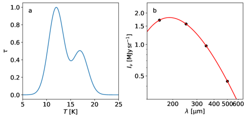
Figure 11: Simulated single-pixel observation. Frame a shows the optical depth distribution as a function of temperature, and frame b shows the SED, with measurements at 160, 250, 350, and 500 $\mu$m.

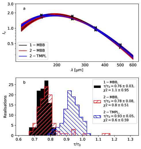
Figure 12: Results from the fitting different noise realisations of the Fig. 11 observations. Frame a shows a few examples of the observations (black crosses) and individual fits (solid curves). Frame b-d show the distributions of $\tau$ estimates (100 noise realisations) for the 1-MBB, 2-MBB, and 3-MBB models, respectively. Each frame quotes the mean value and the standard deviation for the estimates relative to the true value, $\tau/\tau_{0}$.

When the number of observed wavelengths is small, both the 2-TMPL and 2-MBB fits can result in $\chi^{2}$ values below one. This suggests that the $\tau$ estimates may be significantly affected by the noise realisation (as well as any potential priors). The results of Sect. 3.1 showed that a low $\chi^{2}$ value even of the 1-MBB model is not a guarantee of accurate column density estimates. When the number of free parameters is increased, values $\chi^{2}<1$ can be obtained with different parameter combinations. This is illustrated by Fig. 13 that is based on one noise realisation from Fig. 12. This is worse than an average case but illustrates the potential for parameter degeneracies. Figure 13a shows the $\chi 2$ values as a function of the temperatures of two components. The intensities of the components are optimised separately for each pixel in the figure (i.e. for every temperature combination). The plot is reminiscent of the degeneracy of $T-\beta$ fits, with long curved valleys where the minimum $\chi^{2}$ values remain almost constant (cf. Chastenet et al., 2021). Figure 13b shows that fits with $\chi^{2}=1$ correspond to a range of solution, where the difference between the highest and lowest $\tau$ estimates is more than a factor of two. In 2-MBB fits, any of these temperature combinations could be chosen, depending on the priors. In 2-TMPL fits, the solution would be directly dictated by the pre-selected $T_{\rm C}$ values, which might also fall completely outside the $\chi^{2}=1$ contour.

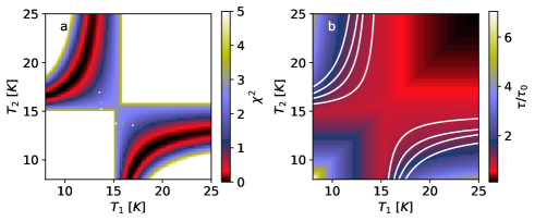
Figure 13: Values of $\chi^{2}$ (frame a) and $\tau/\tau_{0}$ (frame b) as functions of the assumed temperatures $T_{\rm 1}$ and $T_{\rm 2}$ of the fitted SED templates. The observations correspond to one noise realisation selected from the simulations in Fig. 12. Frame b includes contours at $\chi^{2}=0.1$ and $\chi^{2}=1$.

Based on the above, component degeneracies can be a problem already in a two-component model. In multi-component models, these risks are only likely to increase, and feasible solutions with $\chi^{2}\sim 1$ may be reached with many parameter combinations that correspond to different optical depths. In Fig. 14, we simulate 160-500 $\mu$m observations that correspond to a single $T=15$ K MBB spectrum or the sum of two MBB components at 13 K and 17 K. We examined in this case the use of the 10-TMPL model where the $T_{\rm C}$ values are set logarithmically between 8 K to 27 K. We generated random weights for the ten components and registered the combinations that fitted all SED measurements to better than 5% accuracy. Because this is a condition for the maximum error in any of the four bands, it is more strict than the assumption of 3% relative uncertainty that was used in the previous tests. The detailed shapes of the $\tau/\tau_{0}$ distributions (shown in frames c and f) depend on the way the simulation was done. Nevertheless, they show that the recovered $\tau$ values are almost always above the true values. The optical dept can be underestimated only in frame f, when the fit relies on $T_{\rm C}$ components that fall between the true temperatures of 13 K and 17 K. This is another illustration of the obvious fact that four measurements cannot determine 12 parameters in a unique way. Conversely, Fig. 14 can be interpreted to show how the observed sources could have up to a factor of two differences in the optical depths, in spite of showing observationally identical SEDs.

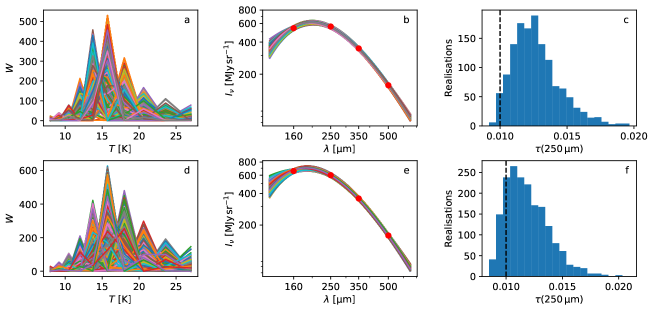
Figure 14: Fits to simulated observations with a 10-TMPL model. The observations consist of 160, 250, 350, and 500 $\mu$m intensities for a single $T=15$ K MBB function (upper frames) or a sum of 13 K and 17 K components of equal optical depth (red circles in frames b and e). Frames a and d show random realisations of the combinations of weights $W$ that result in less than 5% errors for all four predicted intensities (curves in frames b and e). The frames c and f show the distributions of the $\tau$ values predicted by those fits. The true optical depth is $\tau(250\mu{\rm m})=0.01$.

Strict priors can be set only if the nature of the object is well known. If one uses a prior on temperature, such as $T\sim N(T_{0},\delta T)$ in some tests in this paper, the parameters $T_{0}$ and $\delta T$ will clearly be more appropriate for some parts of the maps than for others. Even if $T_{0}$ is varied spatially (e.g. following the temperature from the 1-MBB fit), the parameter $\delta T$ still has a clear effect on the solution (a small $\delta T$ leading to a lower $\tau$). As noted above, the significance of the model errors means that the absolute accuracy of a column density measurement (match to $\tau_{0}$) cannot be judged based on the $\chi^{2}$ values (match to observed intensities). Based on synthetic Herschel 70-500 $\mu$m observations of a cloud simulation, Koepferl et al. (2017) also noted that fits with low $\chi^{2}$ values can correspond to very inaccurate estimates of temperature and column density and, in their case, the fits could entirely fail close to hot sources.

The PPMAP method (Marsh et al., 2015) is another multi-component SED fitting method that uses a combination of SED templates. These can correspond different temperatures (typically a number larger than the number of observed wavelengths) and optionally also to multiple $\beta$ values (e.g. Howard et al., 2019). The model is thus in some respects similar to $N$-TMPL and should be subject to some similar problems of parameter degeneracy. The PPMAP model can use priors for example for the temperature. Furthermore, the program looks for a solution that fits the observations to a $\chi^{2}\sim$1 accuracy with the smallest number of objects in the state space. In a field like the IRDC model it might at each position use only a couple of components that best match the local temperature distribution, also avoiding excessive fitting of minor noise structures in the SEDs. On the other hand, as discussed above, a low number of (SED) components is not a guarantee of unbiased results and the same $\chi^{2}$ value may be reached with different parameter combinations with different predictions of the optical depth. All real source also have continuous temperature distributions, so the number of components needed (and thus also the resulting $\tau$ estimates) will depend on the observational noise.

Figure 15 shows examples of the $\tau$ distributions estimated with MCMC fits. The data are a subset of the IRDC model maps, and the fitted models are 4-TMPL and 2-MBB with the same parameters as in Sect. 3.4. All data are convolved to the same resolution ($18\arcsec$ for an assumed $6\arcsec$ pixel size) to allow faster calculations where each map pixel is fitted separately. These MCMC fits (4-TMPL and 2-MBB models) of the $256\times 256$ pixel maps took each less than ten seconds (with 40000 MCMC steps after the burn-in phase). Therefore, as long as convolution is not part of the model, MCMC remains feasible even for the largest maps. For the assumed 3% observational noise, the typical uncertainty of an individual $\tau$ measurement is less than 50%. However, in those map positions, where the fits underestimate or overestimate the true values the most, the true value is far in the tail of the probability distribution. This is natural since even MCMC gives error estimates only within the confines of the selected model. The uncertainties do not cover the model errors, whether the selected model is appropriate or unique in describing the given data.

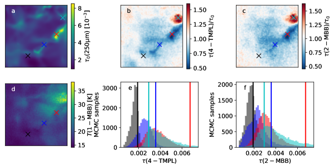
Figure 15: IRDC model observations fitted with MCMC methods. Frame a shows the true $\tau(250\,\mu{\rm m})$ optical depths, and frame d the colour temperature from the 1-MBB fit. Frames b and c show the $\tau$ maps from the 4-TMPL and 2-MBB fits (averages over the MCMC samples) divided by the true optical depth $\tau_{0}$. Frames e and f show the posterior probability distributions for the four positions marked in the b and c frames, and the true values $\tau_{0}$ are indicated with vertical lines of the same colour (black, blue, red, and cyan).

In this paper, $\beta$ was mostly fixed to the value that was used in generating the synthetic observations. If $\beta$ were included as a free parameter in the SED fits, the formal uncertainties of the temperature estimates would increase significantly due to the well-known anti-correlation between the $T$ and $\beta$ parameters (Shetty et al., 2009a; Kelly et al., 2012; Juvela et al., 2013b). Low $\chi^{2}$ values would be concentrated in curved regions in the ($T$, $\beta$) plane, where the observational noise could cause large changes in the best-fit parameters. The large uncertainty in $T$ will directly translate into large uncertainty in $\tau$. The $\chi^{2}$ plane could even exhibit distinct minima that correspond to significantly different temperatures and column density estimates (Juvela & Ysard, 2012a). The $\chi^{2}$ values of the $N$-TMPL and $N$-MBB fits could also exhibit multiple minima, even if $\beta$ we kept constant.

4.5 Correction to MBB fits

Instead of relying on possibly ill-constrained multi-component models, one possibility is to start with the 1-MBB fit and try to mitigate its bias. Juvela et al. (2015b) carried out radiative transfer (RT) modelling of dense clumps and analysed the resulting synthetic surface brightness maps with the 1-MBB method. The ratio between the true optical depth and the optical depth estimated from the synthetic observations was then used to correct the 1-MBB $\tau$ estimates. The accuracy of the correction depends on how well the RT model matches the observed target, and this approach is therefore mainly limited to sources with a simple structure. If the model matched observations perfectly, it would directly provide good estimates for the column density, without the need for any further SED analysis. However, it is more robust to use RT models only to derive fractional corrections that are then applied to 1-MBB results. If the target is spherical (or otherwise geometrically simple), methods like the Abell transformation (Roy et al., 2014) provide a more straightforward and computationally efficient way to estimate the temperature and column density structure of a source. However, a full RT model still has the advantage of presenting a physically self-consistent description of the source, where the temperatures cannot vary in an arbitrary fashion but must be consistent with the radiation sources, the density field, and the resulting attenuation of the radiation field. However, the increased complexity also means that it is more difficult to find a radiative transfer model that would be able to match all observations to the full precision of the observations (Juvela et al., 2013a).

One can ask, whether the observations themselves contain enough information to go beyond the simplest 1-MBB fits. If the measurements do not sufficiently constraint the solution, there will always be significant systematic errors that depend on the construction of the SED models.

The IRDC cloud of Sect. 3.4 is the most complex model examined in this paper, containing large temperature and density gradients. Figure 16a shows again the 1-MBB results where the $\tau$ estimates are in many regions only 50% of the correct value and the maximum errors are close to a factor of five. The main effect of temperature variations is to make the SED broader. With relative differences between the observed intensities and the 1-MBB model fit, $r(\lambda)=(I_{\nu}^{\rm 1-MBB}-I_{\nu}^{\rm observed})/I_{\nu}^{\rm observed}$, we define a parameter

$$\Sigma(\Delta I_{\nu}/I_{\nu})=r(160\,\mu{\rm m})-r(250\,\mu{\rm m})-r(350\,\mu{\rm m})+r(500\,\mu{\rm m}),$$ (11)

which becomes more negative for wider SEDs. Figure 16b-c shows that $\Sigma(\Delta I_{\nu}/I_{\nu})$ is well correlated with the bias of the 1-MBB $\tau$ estimates. In Fig. 16d, the $\tau$ estimates have been corrected for this trend, using a third order polynomial fit to the data in Fig. 16c. This simple empirical correction is successful in eliminating most of the bias, although there is only small improvement towards hot sources. The correction is also more sensitive to noise (being a second-order correction to the 1-MBB fit), which reduces the improvement in the accuracy of individual measurements (as suggested by the dispersion in Fig. 16c). The example shows that the observations do contain more information than used of by the 1-MBB fit alone, but, with the assumed 3% observational noise, there also are limits to the potential improvement.

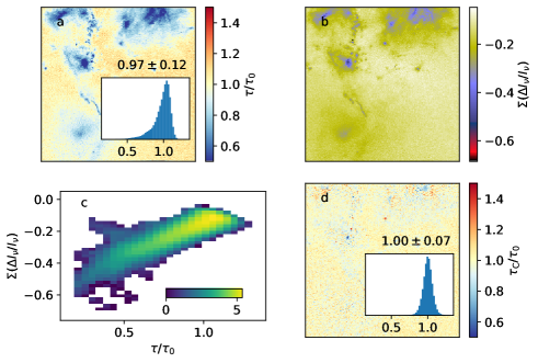
Figure 16: Empirical correction of the 1-MBB optical depth estimates of the IRDC cloud model. Frame a shows the ratio $\tau/\tau_{0}$ between the original estimates and the true optical depths. Frame b shows the quantity $\Sigma(\Delta I_{\nu}/I_{\nu})$ that characterises the difference between each observed spectrum and the 1-MBB fit. Frame c shows the correlation between this quantity and the $\tau$ error, and Frame d shows the $\tau/\tau_{0}$ ratio corrected for the trend in frame c. In frames a and d, the inserts show histograms of the $\tau/\tau_{0}$ values (with linear y-axis). In frame c, the colour scale corresponds to logarithmic point density.

We tested also the use of more general machine learning methods to derive the corrections. A 246$\times$246 pixel part of the IRDC maps was used as the training set for a small, four layers deep neural network. We omitted from the maps only 5-pixel wide border regions that are affected by some edge effects from the beam convolution. The training could be accomplished in a time that is comparable to the previous direct multi-component SED fits, and the trained network can then be used to quickly correct the 1-MBB estimates.

Figure 17 compares the accuracy between the original 1-MBB estimates and the neural-net corrected 1-MBB-NN estimates. For the 246$\times$246 pixel training set, the correction naturally works well. However, it is not perfect, since Fig. 17b still shows faintly the pattern that dominated the errors in the original 1-MBB fits. The trained network was then used to correct data for the full 1875$\times$1875 pixel map (Fig. 17c-d). The result is rather similar to the empirical correction in Fig. 16d. While in Fig. 16 the correction was estimated from the same map where it was then applied, in Fig. 17 the correction was derived from a very small subset ($\sim 1.5$% of the pixels, the rectangle marked in Fig. 17c). The corrected $\tau$ values have a symmetric error distribution. Although there is some positive bias ($\tau/\tau_{0}\sim 1.07\pm 0.09$), the maximum errors have been significantly reduced. This is encouraging regarding the possibility of finding useful corrections, possibly tuned for a given type of sources, that are general enough to be applied also to new observations.

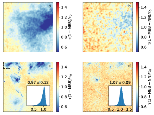
Figure 17: Correction to 1-MBB $\tau$ estimates calculated with neural nets. Frame a shows the 246$\times$246 pixel map that is used as the training set. Frame $c$ shows the 1-MBB results for the whole IRDC map, where the location of the training map is indicated with a dashed box in the upper left corner. Frames b and d shows the corrected $\tau$ maps for the training set and for the full 1875$\times$1875 pixel map, respectively. The lower frames include histograms of the $\tau/\tau_{0}$ values with their mean and standard deviation values.

4.6 Computational cost

The computational cost of the different SED models varied by about four orders of magnitude. Once the data are convolved to the resolution of the longest wavelength observations, the 1-MBB fits of the 1875$\times$1875 maps could be fitted in just a couple of seconds (Appendix A). Even the empirical corrections of Sect. 4.5 would add little to the run times. This can provide a more robust way to estimate optical depths, considering the potential degeneracies in the multi-component fits, although the angular resolution is limited to the lowest common resolution.

When the beam convolution is part of the fit, the run times increase by orders of magnitude. For the $N$-TMPL models only, the optimisation can be done faster in Fourier space (Appendix A). In the case of IRDC maps (1875$\times$1875 pixels and four wavelengths), the run times were of the order of one minute instead of the order of one hour for the fits optimised in the real space. The run times also depend on the chosen convergence criteria. The $\chi^{2}$ values tended to decrease initially fast, with only one or two percent further improvement over a larger number of further iterations.

The beam convolution is a major part of the computational cost. For small maps of up to $\sim 256\times 256$ pixels, the use of a GPU for the FFT computations provides no benefits, but for the largest maps (1875$\times$1875 pixels) the speed-up was a factor of a few. The use of FFTs can cause artefacts at the map boundaries, due to the assumed data periodicity. It is possible to carry out the convolutions in real space, by direct summation of the pixel values over the beams. This gives more freedom in the use of measurement uncertainties (including missing values and potentially even error correlations) and in the handling of the map edges. This remains a viable option for smaller maps, especially when GPUs are used.

The MCMC fitting is typically more time consuming than direct $\chi^{2}$ minimisation. On the other hand, it could provide more complete information of the uncertainties than just using the local $\chi^{2}$ gradients. Some examples of the use of MCMC calculations were given in Figs. 1-3 and in Sect. 4.4, where each map pixel was still fitted separately. However, MCMC turns out to be viable for maps of moderate size even when the beam convolution is part of the model optimisation. Appendix C shows one example, where $320\times 320$ pixel maps are fitted with the 3-TMPL model, the MCMC runs taking about ten minutes on a GPU. The MCMC error estimates are consistent with the observed scatter in the $\tau$ estimates. However, we emphasise again that these formal error estimates, whether based on the $\chi^{2}$ values or MCMC sampling, do not account for the systematic errors that were usually the dominant error component in our tests.

4.7 Further improvements

All fits in Sect. 3 were based on SED models that consist of discrete temperature components. This is not a fundamental limitation, and the basis functions could equally be based on parameterised temperature distributions. Appendix D shows one example, where the SED templates correspond to different Gaussian distributions of the optical depth versus dust temperature. The model parameters are thus the mean value $\langle T\rangle$ and the width $\delta T$ of the temperature distribution and the optical depth. Although the run time was longer (about one hour), the results were in this case also more accurate than those of the 3-TMPL model (Sect. C) that has the same number of free parameters.

The model used in Appendix D is different from both the $N$-TMPL and $N$-MBB ones, and it combines a low number of free parameters with the flexibility of adjusting the mean temperature in a continuous fashion. The MCMC runs used a lookup table of pre-calculated dust spectra. The same approach could be used for any SEDs, which could be based on empirical (e.g. log-normal or broken power laws) or model-based temperature distributions (e.g. Dale et al., 2001; Galliano et al., 2011; Galliano, 2018). For the former, Désert (2022) advocated the use the logarithm of temperature as the more natural parameter. The basis functions could also directly encode prior information, such as the avoidance of unphysically low temperatures.

In this paper we have not considered the possible correlations between the input parameters. If the measurements of the different bands are correlated, the $\chi^{2}$ values are calculated by replacing the sum of $(X_{i}-\hat{X}_{i})^{2}/\sigma(X_{i})^{2}$ values with $(X-\hat{X})\Sigma^{-1}(X-\hat{X})^{T}$, where $X$ are the measured values, $\hat{X}$ the model prediction, and $\Sigma$ the covariance matrix of the observations. With a handful of frequency bands, the effect on the run times would be at most a factor of a few. The spatial correlations of the input data have no effect on the 1-MBB fits, which are done independently for each resolution element. The correlations should nevertheless be taken into account when the data are initially convolved to a common resolution. If the convolution is part of the fitting procedure, the handling of the spatial correlations would have a large impact on the run times. Depending on the beam sizes, each pixel might have non-zero covariances with tens or even hundreds of other pixels. The additional cost would come from the increased complexity in the convolution (to be done now in real space) and in the evaluation of the goodness-of-fit function. The implementation would be more straightforward in the MCMC framework, where the derivatives of the probability function are not needed. However, there would still be significant practical limitations on the size of the maps that could be analysed.

5 Conclusions

We have examined the analysis of dust emission spectra with SED models that consist of $N$-fixed SED templates (models $N$-TMPL, $N>1$) or $N$ MBB functions (models $N$-MBB, $N\geq 1$). Tests with synthetic observations have led to the following conclusions.

• The $N$-TMPL and $N$-MBB models can improve the standard single-component 1-MBB fits, but they require a careful model setup and, in the case of large $N$, the use of appropriate priors.

• The accuracy of the $N$-TMPL models critically depends on the selection of its SED templates. Errors increase rapidly when the temperature of the emission falls outside the temperature range covered by the templates.

• The $N$-MBB models adjust better to large temperature variations in the source maps, but they may need to be combined with priors to avoid very low temperatures that would cause large noise in the $\tau$ estimates. This is true especially if there are many pixels per beam and if the SED of individual pixels is thus not well constrained.

• The fitting of multi-component models is computationally feasible even for large maps, provided that the gradients of the $\chi^{2}$ function are calculated analytically. In our tests, SED fits were performed for maps of up to $1875\times 1875$ pixels.

• When the beam convolution is part of every optimisation step, the use of GPUs can significantly reduce the run times.

• We have presented alternative $N$-TMPL fits that were based on the optimisation in the Fourier space. This results in significant speed-up in the computations, but with some limitations in the use of priors and general error estimates.

• MCMC remains feasible for maps of at least up to $\sim 500\times 500$ pixels (run times of approximately one hour or less), even when each MCMC step includes the convolution of the model-predicted maps. MCMC provides better estimates of the statistical errors, but these do not give any indication of the often larger systematic errors.

• Multi-component fits can contain fundamental degeneracies, where (in the studied cases) the same observed intensities could correspond to a factor of two differences in the true optical depths.

• The bias of the 1-MBB fits can be decreased based on observed data alone by analysing the widening of the SEDs. Neural networks provide a general way to derive such corrections.

The results call for caution when interpreting the results from multi-component SED fits. This is particularly true if the number of free parameters exceeds the number of direct observational constraints and the results thus clearly depend on the chosen priors. Having low $\chi^{2}$ values for the fits does not mean that the corresponding $\tau$ estimates would be correct, but the comparison of alternative SED models can give some indication of the magnitude of the model errors. Our initial results suggest that models with parameterised continuous temperature distributions might perform better than the models (such as $N$-TMPL and $N$-MBB) where only discrete temperatures are used. This needs to be investigated further in a wider range of test cases. Radiative transfer modelling also remains a possibility in the analysis of emission from simple sources, and it is not much more time consuming than the fitting of a complex multi-component SED model.

Appendix A Fitting algorithms

When the beam-convolved model predictions are compared to observations, the fitting is accomplished by minimising the function

$$\chi^{2}=\sum_{i,k}\frac{S_{i,k}-\sum_{c}M_{i,c}\otimes B_{k}}{\delta S_{i,k}^{2}}=\sum_{i,k}\frac{S_{i,k}-{\hat{S}}_{i,k}}{\delta S_{i,k}^{2}},$$ (12)

where $i$ refers to the map position and $k$ to the frequency band, and the model is the sum of multiple components indexed with $c$. The symbol ‘$\otimes$’ stands for the convolution between a model map $M_{i,c}$ and the telescope beam $B_{k}$, and ${\hat{S}}_{k}$ denotes the convolved model predictions. The summation goes over all map positions $i$ and bands $k$.

The functions $M_{i,c}$ are sums of SED components. The $N$-MBB fits use sums of MBB functions

$$M_{i,c,k}=MBB(I_{i,c},T_{i,c},\beta_{i,c})_{i,k},$$ (13)

where $I_{i,c}$ is the intensity at a reference wavelength (see below), and the result is also a function of the band $k$. In this paper, $\beta$ was kept constant and only $I_{i,c}$ and $T_{i,c}$ are considered free parameters. The $N$-TMPL model is somewhat simpler,

$$M_{i,c,k}=W_{i,c}C_{c,k},$$ (14)

with free parameters $W_{i,c,k}$ and the fixed SED templates $C_{c,k}$.

When the $\chi^{2}$ functions is minimised with the conjugate-gradient method, only the function values and the first derivatives with respect to the optimised parameters $X_{i,c}$ are needed. The derivatives with respect to $X_{i_{0},j_{0}}$ can be written as

$$\frac{\partial\chi_{k}^{2}}{\partial X_{i_{0},c_{0}}}=-2\sum_{k}\left[\left(\frac{S_{i,k}-{\hat{S}}_{i,k}}{dS_{i,k}}\right)^{2}\otimes B_{i,k}\right]\frac{\partial M_{i,c,k}}{\partial X_{i_{0},c_{0}}}.$$ (15)

Since the model prediction $\hat{S}$ itself is already the result of convolution, the gradient calculation thus includes two convolution steps. This can be shown by direct derivation of Eq. (12), by replacing the convolution there with an explicit summation over the beam.

The last term in Eq. (15) is the derivative of the model with respect to one of its parameter. In the sum, this is reduced to a single term (pixel $i_{0}$ and component $c_{0}$). If $M$ is the MBB function, it may be numerically beneficial to express it using intensities relative to the value at a suitable reference frequency $\nu_{0}$,

$$M(I,T,\beta)_{i,c,k}=I_{i,c}\,\,\frac{\exp(h\nu_{0}/(kT_{i,c}))-1}{\exp(h\nu/(kT_{i,c}))-1},$$ (16)

where frequency $\nu_{0}$ is the reference frequency and $\nu$ the frequency of the band $k$. The full $M_{i,k}$ function is the sum of the individual components $M_{i,c,k}$. Using the values of the functions $M_{i,c}$ itself, the final partial derivatives in Eq. (15) can be written as

$$\frac{\partial M_{i,c,k}}{\partial I_{i,c}}=M_{i,k}/I_{i,c},$$ (17)

$$\frac{\partial M_{i,c,k}}{\partial T_{i,c}}=\frac{M_{i,k}h\nu}{T_{i,c}^{2}}\left(\frac{\nu}{1-\exp(-h\nu/(kT_{i,c}))}-\frac{\nu_{0}}{1-\exp(-h\nu_{0}/(kT_{i,c}))}\right)$$ (18)

and

$$\frac{\partial M_{i,c,k}}{\partial\beta_{i,c}}=M_{i,c,k}\log(\nu/\nu_{0}),$$ (19)

thus replacing $X_{i_{0},c_{0}}$ with $I$, $T$, or $\beta$. In the case of the $N$-TMPL fits, the derivatives $\partial M/\partial X$ are directly elements of the SED templates

$$\frac{\partial M_{i,c,k}}{\partial W_{i,c}}=C_{i,k}.$$ (20)

The non-negativity of the parameters $I$ could be enforced with an additional penalty function or using an optimisation routine that directly support the use of constraints. We chose to optimise the parameter $\alpha=\log(I)$, which also guarantees the positivity of the intensity values, $I=e^{\alpha}$. For $N$-MBB fits, Eq. (17) becomes in this case

$$\frac{\partial M_{i,c}}{\partial\alpha_{i,c}}=M_{i,c},$$ (21)

where $M$ itself is of course evaluated by replacing $I$ with $\exp(\alpha)$. In the $N$-TMPL fits, all $\partial M/\partial X$ derivatives are of the form

$$\frac{\partial M_{i,c,k}}{\partial W_{i,c}}=e^{W_{i,c}}C_{c,k},$$ (22)

if the original weights $W_{i,c}$ are replaced with terms $e^{W_{i,c}}$.

When the optimisation of the $N$-TMPL model is done in Fourier space (models $N$-TMPL-F), observations $S_{i,k}$ and the weight maps $W_{i,c}$ are replaced in Eq. (12) by their Fourier counterparts and the convolution is replaced by direct multiplication with the Fourier-transformed beams. This is possible because the $N$-TMPL model is linear with respect to SED templates and

$$S_{k}\approx\sum_{c}W_{c}C_{c,k}\Rightarrow{\cal F}(S_{k})\approx\sum_{c}C_{c,k}{\cal F}(W_{c}),$$ (23)

as used in Eq. (8).

The relative run times depend on many factors that include the map size, the number of fitted components, having convolutions as part of the model, and the computational methods used for the convolutions (i.e. either in real space or via FFTs). Figure 18 compares the run time of the 1-MBB fit to 2-MBB, 4-TMPL, and 12-TMPL-F models for maps of different sizes. The observations are for the IRDC model and consist of 160, 250, 350, and 500 $\mu$m maps. The 1-MBB fit is by far the fastest, because the optimisation is done pixel by pixel and model does not include beam convolution. In this case, all maps are first convolved to the same resolution before the SED fitting. The quoted run times are for the optimisation only, and these remain below one second even for the largest maps (when performed on a GPU). The other methods are slower because of the direct additional cost of the convolutions (although that cost is small in case of TMPL-F) and because the convolution connects all parameters and makes the model fitting a more difficult global optimisation problem. The 12-TMPL-F run times correspond to a full run to a converged solution, where all calculations (including the conjugate gradient optimiser) are run on a GPU. In the case of the 2-MBB and 4-TMPL fits, the run times correspond to 13000 function evaluations. This may be sufficient in some cases but a good convergence may require even 2-3 times longer runs. In the 2-MBB and 4-TMPL fits, the optimiser is run on the host machine but the FFT convolutions are performed on a GPU.

As mentioned in Sect. 4.6, FFT calculations were faster on a GPU only for map sizes larger than 256$\times$256 pixels. Because the beam sizes correspond to less than ten pixels (FWHM=36$\arcsec$ at 500 $\mu$m, compared to 6$\arcsec$ pixels), the convolutions could also be done with a GPU in real space, without a drastic increase in the run times. The cost of the real-space convolution also increases only directly proportionally to the map dimensions ($\propto N\times M$) instead of the $NM\log(MN)$ scaling of 2D FFTs.

The calculations for Fig. 18 were performed on a laptop with a discrete GPU (which is nevertheless three generations behind the most recent hardware available). When the optimiser itself was run on the host computer, the run times were mostly bound by the host (the single-threaded program) rather than the FFT calculations on the GPU.

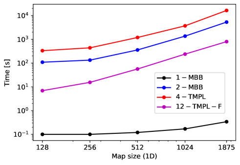
Figure 18: Comparison of run times of different SED fits. The observations are from the IRDC model, and the map size is varied from $128\times 128$ to $1875\times 1875$ pixels. Apart from 1-MBB, beam convolution is always part of model that is being fitted. The number of fitted SED components is given in the legend, and $TMPL-F$ stands for optimisation in the Fourier space.

Appendix B Additional fits of the full IRDC maps

Figure 19 shows 11-TMPL and 4-MBB fits for the whole 1875$\times$1875 pixel maps of the IRDC cloud model. The fit parameters are the same as in Fig. 9 in Sect. 3.4.2, where the smaller 256$\times$256 pixel maps correspond to the upper left corner of these full maps.

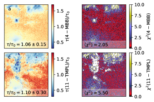
Figure 19: Fits of the 11-TMPL and 4-MBB SED models to full IRDC cloud maps (1875$\times$1875 pixels). The parameters are the same as in Fig. 9.

Section 3.4.3 discussed fits of the 4-TMPL and 12-TMPL models with optimisation in the Fourier space. Figure 20 shows fits for the full 1875$\times$1875 pixel maps using the same parameters.

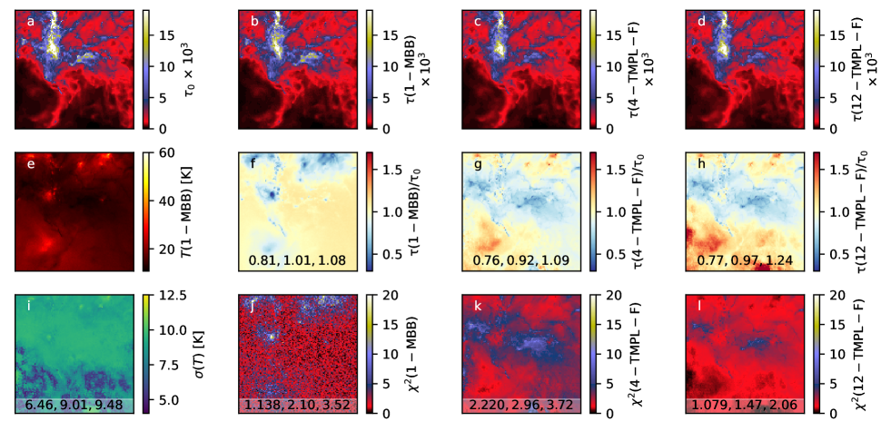
Figure 20: Comparison of 1-MBB fits and 4-TMPL-F and 12-TMPL-F fits performed in Fourier space. The parameters of the fits are the same as in Fig. 9, which corresponded to the upper left corner of the full IRDC maps.

Appendix C MCMC calculations and estimated source sizes

Although MCMC calculations are expected to be more time consuming than direct ML calculations, they turned out to be feasible for maps of moderate size. In the following, we show one example where the fit of the $3-TMPL$ model is done with a basic MCMC simulation. The results are used to examine the estimated source sizes in the case of sources with radial temperature gradients.

The synthetic observations consist of surface brightness maps at 100, 160, 250, 350, and 500 $\mu$m, with angular resolutions of 3, 3, 4.3, and 6.1 pixels, respectively. The background has a temperature of $T_{1}$=15 K and an optical depth of one unit. We add to the maps Gaussian sources that have a size of $FWHM$=20 pixels and a peak optical depth of two units. Each source has a linear temperature gradient from 15 K at the distance of $r=FWHM$ to a lower or a higher temperature $T_{2}$ at the source centre. The temperature $T_{2}$ of the individual sources is varied between 11 K and 19 K. We add to the data white noise that corresponds to 1% relative errors in the surface brightness measurements.

The data were fitted with the 1-MBB model (resolution 6.1 pixels) and with the 3-TMPL model (nominal resolution 3 pixels), using components with $T_{\rm C}$=12.5, 15.0, and 17.5 K. No priors were used, except the requirement of non-negative weights in the 3-TMPL fit. The MCMC calculations of the 3-TMPL model included 200 000 MCMC steps, which was enough for reproducible results.

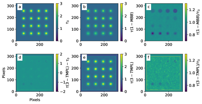
Figure 21: Fits of 1-MBB and 3-TMPL models to maps containing 16 Gaussian sources with different radial temperature gradients. The upper frames show the true value $\tau_{0}$ (frame a), the 1-MBB estimates (frame b), and the ratio of the 1-MBB estimates divided by the true values (frame c). Data in frames b-c have a resolution of 6.1 pixels. The lower frames show results of the 3-TMPL fit: the fit residuals (frame d), the estimated $\tau$ values (frame e), and the ratio of the 3-TMPL estimates and the true values (frame f). The nominal resolution in the lower maps is equal to 3 pixels.

Figure 21 shows a simulation of $320\times 320$ pixel maps that contain 16 Gaussian sources. In the 1-MBB estimates, some residuals are visible for most sources (Fig. 21c). The 3-TMPL fits have a higher resolution but clear errors are visible only a couple of the coldest and warmest sources (Fig. 21d,f).

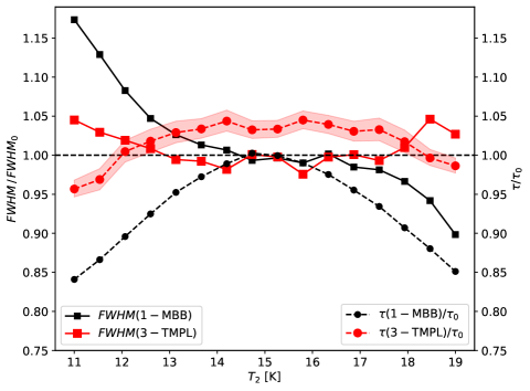
Figure 22: Test with sources with radial temperature gradients. The average optical depth estimates (circles) and the source FWHM estimates (squares) are plotted relative to their correct values. The symbols correspond to 16 sources that are plotted against their central temperature $T_{2}$. The 1-MBB and the 3-TMPL results are plotted in black and red, respectively. The shading shows the MCMC error estimates for the $\tau/\tau_{0}$ ratio in the 3-TMPL fits.

We fitted each of the 16 sources with Gaussians to study the errors in the estimated source sizes. To make the results comparable between the two fits, the 3-TMPL predictions were first convolved down to the resolution of the 1-MBB map. Figure 22 shows the ratios of the estimated and expected beam-convolved FWHM sizes for the 16 sources in Fig. 21. The x-axis corresponds to the temperature $T_{2}$ at the centre of each source. The 1-MBB fits are seen to overestimate the size of the coldest source by $\sim$15% and underestimate the size of the warmest source by 10%. In the 3-TMPL fit the errors remain below $\sim$5%.

We calculated for each source also mean optical depths over and area of 40$\times$40 pixel (twice the source FWHM). Unsurprisingly, the bias of the 1-MBB estimates increases with the temperature difference $|T_{1}-T_{2}|$, and the optical depth is underestimated by up to 15% for both the coldest and warmest sources. The 3-TMPL estimates show a positive bias of $\sim$4%, with values dropping when $T_{2}$ goes outside the range of $T_{\rm C}$ values. Because of noise (and requirement of non-negative component weights) the 3-TMPL model is thus generally slightly overestimating the width of the temperature distribution. The results are on average more accurate than for the 1-MBB model. This is partly due to a better description of the temperature variations and partly due to the higher effective resolution, which reduces the mixing of temperatures within the beam.

Figure 22 also shows the MCMC error estimates for the optical depths. The shaded region corresponds to the interquartile range in the MCMC samples over the 40$\times$40 pixels area around each source. In the plot, the raw error estimates (per resolution element) are scaled down by the ratio between 40 pixels (the averaged area) and nominal resolution of 3 pixels. The MCMC error estimates seem to be consistent with the scatter between the sources (of similar $T_{2}$) but of course does not cover the larger component of systematic errors.

For the above 3-TMPL fit of the 320$\times$320 pixel map, the MCMC run took about ten minutes and is thus not significantly slower than the ML solution. In our tests, the corresponding analysis of 576$\times$576 pixel maps took about half an hour, in agreement with linear dependence on the number of pixels. However, all calculations were done using a GPU, and the run time on a CPU would be at least one order of magnitude longer.

Appendix D MCMC calculations with an alternative SED model

In this paper the $N$-TMPL and $N$-MBB models were based on a set of a few discrete temperatures. However, each template spectrum of the $N$-TMPL models and even the basis functions of the $N$-MBB models could equally be integrals over some temperature distributions.

As a basic example, we tested a three-parameter model where the parameters are the optical depth, the central temperature $T_{\rm C}$ and the width $\delta T$ of a Gaussian temperature distribution. A grid of SED templates was first calculated as the function of $T_{\rm C}$ and $\delta T$. The fitted parameters were the indices to the SED grid and the scaling of the selected template spectrum. As in Sect. C, the model has three free parameters and the fit was performed with MCMC methods. We refer to this as the GRID model.

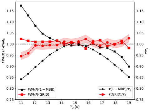
Figure 23: Alternative fit of sources with radial temperature gradients. The symbols are as in Fig. 22, but the red colour and the shaded error regions are for the GRID model.

Figure 23 shows the results for the same synthetic observations as in Sect. C (maps of 320$\times$320 pixels). Because these consist of two discrete temperatures (with spatially varying $T_{2}$), the fitted model of a single Gaussian temperature distribution does not exactly match the simulated data. The results are improved compared to the 3-TMPL fits in Fig. 22, and the $\tau$ values show now very little bias. On the other hand, the run time (on GPUs) is also longer, as the calculation of three MBB functions is replaced by the more time-consuming look-up from a SED table. After an initial burn-in phase, the calculation of 200 000 MCMC steps took one hour.

MCMC calculations provide complete information of the posterior probability of the fitted parameters: the optical depth $\tau$, the mean temperature $\langle T\rangle$, and the width of the temperature distribution $\delta T$. Figure 24 shows examples of these distributions. With the high S/N of the observations assumed in this example, there are no strong correlations between the model parameters.

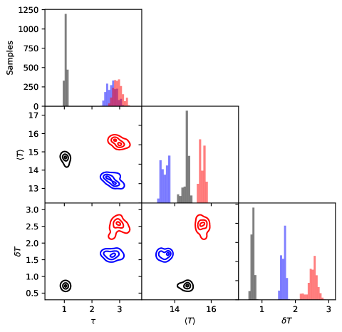
Figure 24: Corner plot showing parameter correlations for three areas in the fits of Fig. 23. The parameters are the optical depth $\tau$, the mean temperature $T_{\rm C}$, and the standard deviation of the temperature distribution $\delta T_{\rm C}$. The data correspond to averages over $3\times 3$ pixels towards the centre of the coldest source (blue), a position in the 15 K background (black), and the centre of the warmest source (red colour). The contours are drawn at 10%, 50%, and 90% of the peak probability density.

Figure 25 compares the power spectra of the different optical depth maps. The analysed region excludes the borders where $\tau$(GRID) solution has not been calculated (cf. Fig. 21f). When the GRID map is convolved to the resolution of the 1-MBB map, the power spectra are nearly identical up to $k\sim 0.05\,{\rm pixel}^{-1}$. We assumed here that, before this convolution, the GRID model would have the nominal resolution of 3 pixels compared to the 6.1 pixel resolution of the 1-MBB model. Figure 25 is approximately consistent with this assumption. The 1-MBB and GRID power spectra separate only at high spatial frequencies, presumably because the GRID solution has a higher statistical noise, even when degraded to the resolution of the 1-MBB solution.

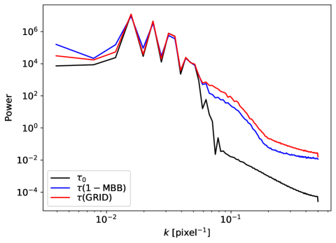
Figure 25: Power spectra of the optical depth maps for the fits in Fig. 23. The spectra are shown for the true optical depth $\tau_{0}$ and the 1-MBB and GRID estimates. For the comparison, the other maps are convolved to the resolution of the 1-MBB map.