Gradient flows of interacting Laguerre cells as discrete porous media flows

Abstract.

We study a class of discrete models in which a collection of particles evolves in time following the gradient flow of an energy depending on the cell areas of an associated Laguerre (i.e. a weighted Voronoi) tessellation. We consider the high number of cell limit of such systems and, using a modulated energy argument, we prove convergence towards smooth solutions of nonlinear diffusion PDEs of porous medium type.

1. Introduction

Voronoi and Laguerre tessellations are a popular approach to describe the neighborhood relations within particle systems, and therefore to model the particle interactions and dynamics. For instance, they have been used as a model for biological cells [13], to describe the regions of influence of different agents in territorial models in ecology [26], or also as discretization tools in continuum mechanics and fluid dynamics [10, 17]. This article focuses on a specific class of models in which the particles evolution in space is governed by the gradient flow of an energy depending on a Laguerre decomposition of a given domain. Our primary interest is to investigate the high number of particles limit of these models, and show how to interpret the particle dynamics as a discrete version of porous media flow, reproducing its Lagrangian gradient flow structure [7]. Adopting this point of view, we will establish quantitative estimates for the convergence of the discrete models to their continous counterparts.

1.1. Problem description

Given $N\in\mathbb{N}$, a tessellation $\mathcal{L}=\{L_{1},\ldots,L_{N}\}$ of a measurable set $A\subset\mathbb{R}^{d}$ is a collection of a finite number of measurable subsets $L_{i}\subset A$, called cells, such that

$$\mathrm{int}(L_{i})\cap\mathrm{int}(L_{j})=\varnothing\quad\forall\,i\neq j\,,\quad\text{and}\quad\cup_{i}L_{i}=A.$$

We call $\mathbb{T}_{N}(A)$ the set of tessellations of $A$ composed of $N$ cells, and

$$\mathbb{T}_{N}^{s}(A)\coloneqq\{\mathcal{L}\in\mathbb{T}_{N}(B)\,:\,B\subseteq A\}\,.$$

Given a compact domain $\Omega\subset\mathbb{R}^{d}$ with Lipschitz boundary, we study the dynamics of $N$ interacting cells, represented by a tessellation in $\mathbb{T}_{N}^{s}(\Omega)$, and whose location is parameterized by a vector of cell centers (or particles) $X=(x_{1},\ldots,x_{N})\in{(\mathbb{R}^{d})}^{N}$. Specifically, for a given subset of admissible tessellations $\mathbb{L}_{N}(\Omega)\subseteq\mathbb{T}_{N}^{s}(\Omega)$ and a fixed parameter $\varepsilon>0$, we consider the following energy:

(1.1) $$F_{\varepsilon}(X)\coloneqq\inf_{\mathcal{L}\in\mathbb{L}_{N}(\Omega)}\sum_{i}\int_{L_{i}}\frac{|x-x_{i}|^{2}}{2\varepsilon}\,\mathrm{d}x+\sum_{i}C_{i}(|L_{i}|)\,.$$

In practice, we will focus on the two cases where $\mathbb{L}_{N}(\Omega)$ is either $\mathbb{T}_{N}(\Omega)$ (the union of the cells is fixed) or $\mathbb{T}_{N}^{s}(\Omega)$ (the union of the cells is optimal). Loosely speaking, the first term in (1.1) measures how close the tessellation is representative of the particle distributions. The second term is the energy of the tessellation which we suppose to depend only on the cell volumes, $C_{i}:[0,\infty)\rightarrow\mathbb{R}$ being a given function which might be different for each cell. For example, a common choice for $C_{i}$ used to model biological cells, is the (non)linear spring model

$$C_{i}(a)=C(a)=K(a)\frac{|a-\bar{a}|^{2}}{2}\,\quad\forall\,i\,,$$

where $K(a)>0$ is a scaling factor called bulk modulus and which might depend on $a$, and $\bar{a}>0$ is the target volume which is assumed common to all cells. The dynamics of the cell centers on the time interval $[0,T]$ is governed by the gradient flow of $F_{\varepsilon}$, with respect to a weighted $l^{2}$ metric on $(\mathbb{R}^{d})^{N}$, defined as follows:

(1.2) $$\langle\dot{X},\dot{Y}\rangle_{m^{0}}\coloneqq\sum_{i}m_{i}^{0}\langle\dot{x}_{i},\dot{y}_{i}\rangle$$

for all $\dot{X},\dot{Y}\in(\mathbb{R}^{d})^{N}$ and where $m^{0}\coloneqq\{m_{1}^{0},\ldots,m^{0}_{N}\}\in\mathbb{R}^{N}_{>0}$. More precisely the evolution of the cell centers is given by a curve $X:[0,T]\rightarrow(\mathbb{R}^{d})^{N}$ satisfying

(1.3) $$\dot{X}(t)=-\nabla_{m^{0}}F_{\varepsilon}(X(t))$$

for all $t\in(0,T)$, with a given initial condition $X(0)=X^{0}=(x^{0}_{i})\in\Omega^{N}$, where $\nabla_{m^{0}}$ denotes the gradient with respect to (1.2).

1.2. Relation with Laguerre tessellations and other discrete models

A Laguerre tessellation (also called power diagram or weighted Voronoi tessellation) is a tessellation of the domain $\mathcal{L}(X,w)=\{L_{i}(X,w)\}_{i}\in\mathbb{T}_{N}(\Omega)$ parameterized by a set of particles $X=(x_{1},\ldots,x_{N})\in(\mathbb{R}^{d})^{N}$ and associated weights $w=(w_{1},\ldots,w_{N})\in\mathbb{R}^{N}$, and in which the cells $L_{i}(X,w)\subset\Omega$ are defined as follows

$$L_{i}(X,w)\coloneqq\{x\in\Omega\,:\,|x-x_{i}|^{2}-w_{i}\leq|x-x_{j}|^{2}-w_{j}\,\quad\forall j\neq i\}\,.$$

We will also refer to $x_{i}$ as the cell center of the cell $L_{i}(X,w)$. Note that if $w$ is a constant vector then we retrieve the standard Voronoi tessellation of $\Omega$.

The Voronoi tessellation can be shown to be the unique minimizer of the energy (1.1) when $C_{i}=0$ and $\mathbb{L}_{N}(\Omega)=\mathbb{T}_{N}(\Omega)$. In this case, the remaining term in (1.1) is sometimes referred to as centroidal Voronoi tessellation energy [18], and the resulting model governed by (1.3) coincides with the Voronoi liquid described in [24], which is a fluid dynamic interpretation of the Lloyd’s algorithm [19, 21].

In general, the optimal tessellations for problem (1.1) with $\mathbb{L}_{N}(\Omega)=\mathbb{T}_{N}(\Omega)$ is always a Laguerre tessellation, and when $\mathbb{L}_{N}(\Omega)=\mathbb{T}^{s}_{N}(\Omega)$ is contained in one (in particular each cell of the optimal tessellation is the intersection of a Laguerre cell with a ball); see Section 2. Our discrete model is therefore related to cell evolution models based on Laguerre tessellations [14]. In Voronoi cell models, for example, one imposes the tessellation to be Voronoi and the energy of the system only contains the second term in (1.1) (plus extra energy terms often related to the cell perimeter or nodes distance). Estabilishing continuous limit for such models is not trivial, partly because the energies considered are usually more complex than those we treat here. Available results are therefore limited to 1d [8] or formal calculations [1]. In this light, the energy (1.1) leads to a modified dynamics which is however more amenable to theoretical analysis, at least for the case of energies only depending on the cell area.

1.3. Relation with Lagrangian discretizations of porous media flow

In the following, we focus on the case where

(1.4) $$C_{i}(a)\coloneqq\left\{\begin{array}[]{ll}\displaystyle U\left(\frac{m_{i}^{0}}{a}\right)a&\text{if }a>0\\ +\infty&\text{otherwise}\end{array}\right.$$

where $U:[0,\infty)\rightarrow\mathbb{R}$ is a smooth strictly convex function with superlinear growth, with $U(0)=0$. For this energy, the particle dynamics generated by (1.3) can be reinterpreted as a spatially discrete version of the Lagrangian formulation of the porous medium equation, describing the evolution of a density $\rho:[0,T]\times\Omega\rightarrow[0,\infty)$ as the solution of the PDE:

(1.5) $$\left\{\begin{array}[]{ll}\partial_{t}\rho-\mathrm{div}\left[\rho\nabla U^{\prime}(\rho)\right]=0&\text{ on }(0,T)\times\Omega\,,\\ \nabla U^{\prime}(\rho)\cdot n_{\partial\Omega}=0&\text{ on }(0,T)\times\partial\Omega\,,\end{array}\right.$$

where $n_{\partial\Omega}$ denotes the unit normal to the boundary $\partial\Omega$, with given initial conditions $\rho(0,\cdot)=\rho^{0}$.

To make this precise, let us fix a smooth strictly-positive reference density $\nu:\Omega\rightarrow(0,\infty)$, and consider the energy $\mathcal{F}:\mathrm{Diff}(\Omega)\rightarrow\mathbb{R}$ on the space of diffeomorphisms of $\Omega$, defined by

(1.6) $$\mathcal{F}(\varphi)=\int_{\Omega}U\left(\frac{\nu}{\mathrm{det}(\nabla\varphi)}\right)\circ\varphi^{-1}\,.$$

Given $\Phi\in\mathrm{Diff}(\Omega)$ such that

(1.7) $$\rho^{0}=\frac{\nu}{\mathrm{det}(\nabla\Phi)}\circ\Phi^{-1}\,,$$

one can check that, at least formally, the flow $\varphi:[0,T]\rightarrow\mathrm{Diff}(\Omega)$ of the vector field $-\nabla U^{\prime}(\rho)$ solves the gradient flow system

(1.8) $$\left\{\begin{array}[]{l}\partial_{t}\varphi(t)=-\nabla_{\mathbb{F}}\mathcal{F}(\varphi(t))\\ \varphi(0)=\Phi\end{array}\right.\text{ and }\quad\rho(t)=\frac{\nu}{\det\nabla\varphi(t)}\circ\varphi(t)^{-1}\,,$$

where $\mathbb{F}\coloneqq L^{2}_{\nu}(\Omega;\mathbb{R}^{d})$ and therefore $\nabla_{\mathbb{F}}$ is the gradient computed with respect to the $L^{2}$ inner product weighted by $\nu$ (see [7] for details on this interpretation, or also Section 3).

Let us now fix a tessellation $\mathcal{T}_{N}=\{T_{i}\}_{i}\in\mathbb{T}_{N}(\Omega)$, and let $\mathbb{F}_{N}$ be the space of piecewise constant functions on the triangulation with values in $\mathbb{R}^{d}$, i.e.

$$\mathbb{F}_{N}\coloneqq\{\varphi^{X}\in\mathbb{F}:\varphi^{X}(x)=x_{i}\in\mathbb{R}^{d}~{}\text{ for a.e.\ }x\in T_{i}\}.$$

Any element $\varphi^{X}\in\mathbb{F}_{N}$ can be identified with a collection of particles $X=(x_{i})_{i}\in(\mathbb{R}^{d})^{N}$ given by the collection of images of the cells $T_{i}$. Then, a general strategy to construct a particle discretization of equation (1.8) is to look for solutions $\varphi^{X}:[0,T]\rightarrow\mathbb{F}_{N}$ of

(1.9) $$\partial_{t}\varphi^{X}(t)=-\nabla_{\mathbb{F}_{N}}\tilde{\mathcal{F}}(\varphi^{X}(t))$$

where $\tilde{\mathcal{F}}:\mathbb{F}_{N}\rightarrow\mathbb{R}$ is an approrpiate discrete version of $\mathcal{F}$, and with $\varphi^{X}(0)$ being an approximation of $\Phi$ in $\mathbb{F}_{N}$. Different choices of $\tilde{\mathcal{F}}$ lead to different methods. We refer to [4] for a review of possible strategies in this context (see in particular [5], for an approach that is particularly close to the one we study in this article). Importantly, our discrete model (1.3) is equivalent to (1.9) for an appropriate variational regularization of the energy (see again Section 3 for details). Such a regularization is related to recent approaches based on semi-discrete optimal transport recalled in Section 1.4.

1.4. Relation with semi-discrete optimal transport

The energy in (1.1) admits a reformulation based on semi-discrete optimal transport [22]. In fact, denoting by $W_{2}(\mu_{1},\mu_{2})$ the $L^{2}$-Wasserstein distance between two positive measures $\mu_{1},\mu_{2}\in\mathcal{M}_{+}(\Omega)$, one can show that if $x_{i}\neq x_{j}$ for all $i\neq j$,

(1.10) $$F_{\varepsilon}(X)=\inf_{a\in\mathbb{R}^{N}_{>0},\eta\in\mathcal{C}}\frac{W_{2}^{2}\Big{(}\sum_{i}a_{i}\delta_{x_{i}},\eta\Big{)}}{2\varepsilon}+\sum_{i}U\left(\frac{m^{0}_{i}}{a_{i}}\right){a_{i}}\,,$$

where we used for $C_{i}$ the expression given in (1.4), and where $\mathcal{C}$ is a convex subset of $\mathcal{M}_{+}(\Omega)$: in particular, $\mathcal{C}=\{{\mathrm{d}x}\}$ (where ${\mathrm{d}x}$ is the Lebesgue measure on $\Omega$) if $\mathbb{L}_{N}(\Omega)=\mathbb{T}_{N}(\Omega)$, and $\mathcal{C}=\{f\mathrm{d}x\,:\,f:\Omega\rightarrow[0,1]\}$ if $\mathbb{L}_{N}(\Omega)=\mathbb{T}_{N}^{s}(\Omega)$ (see Appendix A for a proof).

Equation (1.10) highlights a link with a different approach which consists in regarding the energy of the system (1.6) as a function of the density, and considering its Moreau-Yosida regularization on the space of positive measures measures $\mathcal{M}_{+}(\Omega)$ with fixed total mass, with respect to the $W_{2}$ distance. This yields:

(1.11) $$\tilde{F}_{\varepsilon}(X)\coloneqq\inf_{\rho\in\mathcal{M}^{ac}_{+}(\Omega)}\frac{W_{2}^{2}\Big{(}\sum_{i}m^{0}_{i}\delta_{x_{i}},\rho\Big{)}}{2\varepsilon}+\int_{\Omega}U(\rho)\,,$$

where $\mathcal{M}^{ac}_{+}(\Omega)$ is the set of absolutely continuous positive measures on $\Omega$. The orginal idea of these type of energy regularizations stems from the work of Brenier in [3] for discretizing the incompressible Euler equations, and its more recent reformulation using semi-discrete optimal transport in [20, 9]. The energy (1.11) was then used in [10, 17] to discretize the same nonlinear diffusion models considered in this article as well as the compressible (barotropic) Euler equations, and in [25] in the context of mean field games.

Note that the advantage of using (1.10) with respect to (1.11) is that the first implies a piece-wise constant density reconstruction (see equation (1.12) below) which is easier to handle numerically than the minimizers of (1.11) whose structure strongly depends on $U$. Moreover the variational definition (1.11) is also easier to generalize to more complex energies (see Remark 3.1). Finally, we remark that another discretization strategy similar to ours, which also leads to piece-wise constant densities on Laguerre cells, was proposed in [2], but the aim of this latter work was not to derive quantitative convergence estimates as we do here.

1.5. Continuous limit

For a given initial condition $X^{0}\in\Omega^{N}$ such that $x^{0}_{i}\neq x^{0}_{j}$ for all $i\neq j$, let $t\in[0,T]\mapsto X(t)$ solve system (1.3) with energy (1.4) and

$$m^{0}_{i}=\int_{T_{i}}\nu=\int_{\Phi(T_{i})}\rho^{0}$$

where $\rho^{0}$ satisfies (1.7) as before. Consider the discrete density

(1.12) $$\bar{\mu}_{N}(t,\cdot)\coloneqq\sum_{i}\frac{m^{0}_{i}}{|L_{i}(t)|}\boldsymbol{1}_{L_{i}(t)}$$

where $L_{i}(t)$ is the unique (see Section 2.2) optimal tessellation for problem (1.1) associated with the positions $X(t)$, and where $\boldsymbol{1}_{L_{i}(t)}$ is the indicator function of the set $L_{i}(t)$. Our main result states that $\bar{\mu}_{N}$ converges to sufficiently smooth solutions $\rho$ of (1.5) as long as the error in the initial conditions, measured by

(1.13) $$\delta_{N}^{2}\coloneqq\sum_{i}\int_{T_{i}}|\Phi(x)-x_{i}^{0}|^{2}\nu(x)\mathrm{d}x\,,$$

and $\varepsilon$ go to zero with appropriate rates.

Theorem 1.1.

Let $U:[0,\infty)\rightarrow\mathbb{R}$ be a smooth strictly convex function, with $U(0)=0$, verifying the assumptions of Lemma 4.1 and suppose that there exist $R,\alpha>1$ and $\beta>0$, such that

$$U(r)-\inf U\geq\beta r^{\alpha}\quad\forall\,r\geq R\,.$$

Suppose that $\rho:[0,T]\times\Omega\rightarrow[0,\infty)$ is a strong solution to (1.5), such that $\rho^{0}:\Omega\rightarrow[\rho_{min},\infty)$ with $\rho_{min}>0$ is of class $C^{1,1}$ and verifies (1.7), and $\nabla U^{\prime}(\rho)$ is of class $C^{2,1}$ in space, uniformly in time. Moreover, let $\bar{\mu}_{N}:[0,T]\times\Omega\rightarrow[0,\infty)$ be the discrete solution defined in (1.12) via system (1.3), with energy defined using (1.4). Then

(1.14) $$\max_{t\in[0,T]}\int_{\Omega}U(\bar{\mu}_{N}(t,\cdot)|\rho(t,\cdot))\leq C\left(\frac{\delta_{N}^{2}}{\varepsilon}+\varepsilon^{p-1}\right)\,,$$

where $p=\min\{2,\alpha\}$, $U(r|s)\coloneqq U(r)-U(s)-U^{\prime}(s)(r-s)$ for all $r\geq 0$ and $s>0$, and where the constant $C>0$ only depends on $\sup_{t\in[0,T]}\|\nabla U^{\prime}(\rho(t,\cdot)\|_{C^{2,1}}$, $\|\rho^{0}\|_{C^{1,1}}$, $\rho_{min}$, $\mathrm{diam}(\Omega)$, $U$, $T$, and $d$.

The proof is contained in Section 4. Just as in [10], it relies on a Grönwall argument applied on an appropriately constructed modulated energy (as in the classical approach to obtain weak strong stability results on (1.5); see, e.g., Chapter 5 in [6]). The error estimate we prove is actually stronger than (1.14), and it is given explicitly in equation (4.16) (see also Section 4.7 for an extension in the presence of external potentials). In particular, the same bound holds for the error in the $L^{2}_{\nu}$ norm between the exact Lagrangian flow (according to the interpretation described in Section 1.3) and the discrete one, given by the collection of the particle trajectories. Finally, note that if for example we set

(1.15) $$x^{0}_{i}=\mathrm{arg}\min_{y\in\mathbb{R}^{d}}\int_{T_{i}}|\Phi(x)-y|^{2}\nu(x)\mathrm{d}x\,,$$

then $\delta_{N}$ is just the $L^{2}_{\nu}$ projection error of $\Phi$ onto $\mathbb{F}_{N}$, the space of piece-wise constant vector fields on $\mathcal{T}_{N}$. Hence, denoting by $h_{N}=\max_{i}\mathrm{diam}(T_{i})$ the largest cell diameter, we have $\delta_{N}\leq\|\nabla\Phi\|_{\infty}(\rho^{0}[\Omega])^{1/2}h_{N}$, where $\rho^{0}[\Omega]$ is the integral of $\rho^{0}$ over $\Omega$.

2. Analysis of the discrete model

In this section, we describe in more detail the discrete model (1.3), in particular we explain the link with Laguerre tessellations and provide an explicit formula for the gradient of the energy with respect to the particle positions. While much of the analysis follows the same lines as in [17], or is based on standard arguments from semi-discrete optimal transport (see Appendix A or [22], for example), we provide the proofs of the main statements without using directly optimal transport theory, for the sake of clarity and to make the discussion self-contained.

2.1. Internal energy

We suppose that the functions $C_{i}$ defining the energy of the tessellation are given by

$$C_{i}(a)\coloneqq\left\{\begin{array}[]{ll}\displaystyle U\left(\frac{m_{i}^{0}}{a}\right)a&\text{if }a>0\\ +\infty&\text{otherwise}\end{array}\right.$$

where $U:[0,\infty)\rightarrow\mathbb{R}$ is a smooth strictly convex function with superlinear growth, with $U(0)=0$. From this, it is easy to deduce that $C_{i}$ is strictly convex, decreasing and

$$C_{i}(a)\rightarrow m^{0}_{i}U^{\prime}(0)\quad\text{ as }\quad a\rightarrow+\infty.$$

As a consequence $C^{*}_{i}:\mathbb{R}\rightarrow(-\infty,\infty]$ is also strictly convex. More precisely, $\mathrm{dom}(C^{*}_{i})\subseteq(-\infty,0]$ and $C^{*}_{i}$ is an increasing diffeomorphism between $(-\infty,0)$ and $(-\infty,-m_{i}U^{\prime}(0))$ and $(C^{*}_{i})^{\prime}(0)=+\infty$ (since $C_{i}$ is finite on $(0,\infty)$).

The pressure function associated with $U$ is the strictly increasing function $P:[0,\infty)\rightarrow[0,\infty)$, defined by

(2.1) $$P(r)=\left\{\begin{array}[]{ll}rU^{\prime}(r)-U(r)&\text{ if }r>0\\ 0&\text{ if }r=0\end{array}\right.$$

and satisfying $P^{\prime}(r)=rU^{\prime\prime}(r)$ for all $r>0$. This is related to $C_{i}^{\prime}$ and $C^{*}_{i}$ by

(2.2) $$C^{\prime}_{i}(a)=-P\left(\frac{m_{i}^{0}}{a}\right)\quad\text{and}\quad(C^{*}_{i})^{\prime}(w)=\frac{m_{i}^{0}}{P^{-1}(-w)}\,,$$

for all $a>0$ and $w<0$.

2.2. Dual formulation

From now on we suppose that $X=(x_{1},\ldots,x_{N})\in(\mathbb{R}^{d})^{N}$ is given and that $x_{i}\neq x_{j}$ for all $i\neq j$. First we rewrite the energy (1.1) as follows:

(2.3) $$F_{\varepsilon}(X)=\inf_{\mathcal{L}\in\mathbb{L}_{N}(\Omega),a\in\mathbb{R}^{N}}\sup_{w\in\mathbb{R}^{N}}\sum_{i}\int_{L_{i}}\frac{|x-x_{i}|^{2}}{2\varepsilon}\,\mathrm{d}x+C_{i}(a_{i})+\frac{w_{i}}{2\varepsilon}(a_{i}-|L_{i}|)\,.$$

We obtain the dual problem by swapping the inf and the sup,

$$D_{\varepsilon}(X) \coloneqq\sup_{w\in\mathbb{R}^{N}}\inf_{\mathcal{L}\in\mathbb{L}_{N}(\Omega),a\in\mathbb{R}^{N}}\sum_{i}\int_{L_{i}}\frac{|x-x_{i}|^{2}}{2\varepsilon}\,\mathrm{d}x+C_{i}(a_{i})+\frac{w_{i}}{2\varepsilon}(a_{i}-|L_{i}|)$$

$$=\sup_{w\in\mathbb{R}^{N}}\inf_{\mathcal{L}\in\mathbb{L}_{N}(\Omega)}\sum_{i}\int_{L_{i}}\frac{|x-x_{i}|^{2}-w_{i}}{2\varepsilon}\,\mathrm{d}x-C_{i}^{*}\left(-\frac{w_{i}}{2\varepsilon}\right)\,.$$

Let $\phi(w;\cdot):\Omega\rightarrow\mathbb{R}$ be the function defined by $\phi(w;x)=\mathrm{min}_{i}|x-x_{i}|^{2}-w_{i}$. If $\mathbb{L}_{N}(\Omega)=\mathbb{T}_{N}^{s}(\Omega)$, then $\mathcal{L}\in\mathbb{T}_{N}(\tilde{\Omega})$ for some $\tilde{\Omega}\subseteq\Omega$, and

$$\sum_{i}\int_{L_{i}}\frac{|x-x_{i}|^{2}-w_{i}}{2\varepsilon}\mathrm{d}x \geq\frac{1}{2\varepsilon}\int_{\tilde{\Omega}}\phi(w;x)\,\mathrm{d}x$$

$$\geq\frac{1}{2\varepsilon}\int_{\Omega}\min(0,\phi(w;x))\,\mathrm{d}x$$

$$=\sum_{i}\int_{L^{s}_{i}(X,w)}\frac{|x-x_{i}|^{2}-w_{i}}{2\varepsilon}\mathrm{d}x\,,$$

where

(2.4) $$L^{s}_{i}(X,w)\coloneqq L_{i}(X,w)\cap B(x_{i},(w_{i}^{+})^{1/2})\,,$$

where $B(x_{i},(w_{i}^{+})^{1/2})$ is the closed ball of radius $w_{i}^{1/2}$ if $w_{i}\geq 0$, and $\varnothing$ otherwise. On the other hand if $\mathbb{L}_{N}(\Omega)=\mathbb{T}_{N}(\Omega)$, by the same argument we obtain

$$\sum_{i}\int_{L_{i}}\frac{|x-x_{i}|^{2}-w_{i}}{2\varepsilon}\mathrm{d}x\geq\sum_{i}\int_{L_{i}(X,w)}\frac{|x-x_{i}|^{2}-w_{i}}{2\varepsilon}\mathrm{d}x\,.$$

Therefore

(2.5) $$D_{\varepsilon}(X)=\sup_{w\in\mathbb{R}^{N}}D_{\varepsilon}(X;w)\,,$$

where

$$D_{\varepsilon}(X;w)\coloneqq\sum_{i}\int_{L_{i}^{*}(X,w)}\frac{|x-x_{i}|^{2}-w_{i}}{2\varepsilon}\,\mathrm{d}x-C_{i}^{*}\left(-\frac{w_{i}}{2\varepsilon}\right)\,.$$

and

$$L_{i}^{*}(X,w)=\left\{\begin{array}[]{ll}L_{i}(X,w)&\text{ if }\mathbb{L}_{N}(\Omega)=\mathbb{T}_{N}(\Omega)\\ L_{i}^{s}(X,w)&\text{ if }\mathbb{L}_{N}(\Omega)=\mathbb{T}_{N}^{s}(\Omega)\end{array}\,.\right.$$

A graphical representation of an optimal tessellation in the case $\mathbb{L}_{N}(\Omega)=\mathbb{T}_{N}^{s}(\Omega)$ is given in Figure 1.

Figure 1. An example of optimal tessellation with cells constructed via equation (2.4).

Proposition 2.1.

The function $D_{\varepsilon}(X;\cdot):\mathbb{R}^{N}\rightarrow(-\infty,\infty]$ is concave and $C^{1}$ on its effective domain $\mathrm{dom}(D_{\varepsilon}(X;\cdot))\subseteq[0,\infty)^{N}$. In particular for all $w\in(0,\infty)^{N}$,

$$\partial_{w_{i}}D_{\varepsilon}(X;w)=\frac{1}{2\varepsilon}(C_{i}^{*})^{\prime}\left(-\frac{w_{i}}{2\varepsilon}\right)-\frac{|L_{i}^{*}(X,w)|}{2\varepsilon}\,\quad\forall\,i.$$

Furthermore there exists a unique $w^{*}\in(0,\infty)^{N}$ such that $\partial_{w_{i}}D_{\varepsilon}(X;w^{*})=0$ for all $i$, or equivalently

(2.6) $$P\left(\frac{m^{0}_{i}}{|L_{i}^{*}(X,w)|}\right)=\frac{w_{i}}{2\varepsilon}\,\quad\forall\,i\,,$$

and therefore maximising $D_{\varepsilon}(X;\cdot)$.

Proof.

The concavity and $C^{1}$ regularity of $D_{\varepsilon}(X;\cdot)$ can be proven using standard arguments from the theory of semi-discrete optimal transport [22]. In particular, consider the function

$$Q(w)\coloneqq\sum_{i}\int_{L_{i}^{*}(X,w)}\frac{|x-x_{i}|^{2}-w_{i}}{2\varepsilon}\,\mathrm{d}x$$

and observe that for any $w,\tilde{w}\in\mathbb{R}^{N}$

$$Q(\tilde{w})\leq\sum_{i}\int_{L_{i}^{*}(X,w)}\frac{|x-x_{i}|^{2}-\tilde{w}_{i}}{2\varepsilon}\,\mathrm{d}x=Q(w)+\sum_{i}\frac{w_{i}-\tilde{w}_{i}}{2\varepsilon}|L_{i}^{*}(X,w)|\,.$$

This shows that the super-differential of $Q$ at $w$ is not empty since the vector $(-|L_{i}^{*}(X,w)|/(2\varepsilon))_{i}\in\partial^{+}Q(w)$, and therefore $Q$ is concave. Furthermore, since $|L_{i}^{*}(X,w)|$ is a continuous function of $w$ (see, e.g., Proposition 38 in [22]), $Q$ (and therefore $D_{\varepsilon}(X;\cdot)$) is necessarily $C^{1}$. Existence of maximizers can be shown oberving that the function $D_{\varepsilon}(X;\cdot)$ is coercive since for any $j$,

$$\sum_{i}\int_{L^{*}_{i}(X,w_{i})}\frac{|x-x_{i}|^{2}-w_{i}}{2\varepsilon}\mathrm{d}x\leq\int_{\Omega}\frac{|x-x_{j}|^{2}-w_{j}}{2\varepsilon}\mathrm{d}x\leq\frac{\mathrm{diam}(\Omega)^{2}}{2\varepsilon}|\Omega|-\frac{|\Omega|}{2\varepsilon}w_{j}\,.$$

Since $(C^{*}_{i})^{\prime}(0)=+\infty$ we get that necessarily $w_{i}>0$, so the optimality conditions hold. Uniqueness of maximizers is a consequence of the strict convexity of the functions $C_{i}^{*}$. ∎

From Proposition 2.1, we can deduce the equivalence with the primal problem (1.1), and the existence and uniquess of solutions for this latter. In fact, denoting by $w^{*}$ the unique solution of $\partial_{w_{i}}D_{\varepsilon}(X;w^{*})=0$ for all $i$, then

$$D_{\varepsilon}(X;w^{*}) =\sum_{i}\int_{L_{i}^{*}(X,w^{*})}\frac{|x-x_{i}|^{2}}{2\varepsilon}\,\mathrm{d}x-\frac{w_{i}^{*}}{2\varepsilon}(C_{i}^{*})^{\prime}\left(-\frac{w_{i}^{*}}{2\varepsilon}\right)-C_{i}^{*}\left(-\frac{w_{i}}{2\varepsilon}\right)$$

$$=\sum_{i}\int_{L_{i}^{*}(X,w^{*})}\frac{|x-x_{i}|^{2}}{2\varepsilon}\,\mathrm{d}x+C_{i}(|L_{i}^{*}(X,w^{*})|)\geq F_{\varepsilon}(X).$$

Since $w^{*}$ is the unique maximizer of the dual problem (2.5), this also implies that the tessellation $\mathcal{L}^{*}(X,w^{*})\coloneqq\{L_{i}^{*}(X,w^{*})\}_{i}$ is the unique solution to problem (1.1).

In the following we will need the optimality conditions in Proposition 2.1 in the following alternative form:

Lemma 2.2.

Let $\mathcal{L}=\{L_{i}\}_{i}$ solve problem (1.1), with $\mathbb{L}_{N}(\Omega)$ equal to either $\mathbb{T}_{N}(\Omega)$ or $\mathbb{T}_{N}^{s}(\Omega)$. Then for any smooth vector field $u:\Omega\rightarrow\mathbb{R}^{d}$ with $u\cdot n_{\partial\Omega}=0$ on $\partial\Omega$,

$$\sum_{i}\int_{L_{i}}\frac{x-x_{i}}{\varepsilon}\cdot u(x)\,\mathrm{d}x=\sum_{i}\int_{L_{i}}\left[P\left(\frac{m_{i}^{0}}{|L_{i}|}\right)-\frac{|x-x_{i}|^{2}}{2\varepsilon}\right]\mathrm{div}u(x)\,\mathrm{d}x$$

Proof.

Consider again the function $\phi(w;\cdot):\Omega\rightarrow\mathbb{R}$ defined by $\phi(w;x)=\mathrm{min}_{i}|x-x_{i}|^{2}-w_{i}$. If $\mathbb{L}_{N}(\Omega)=\mathbb{T}_{N}(\Omega)$ we have

$$\sum_{i}\int_{L_{i}}\frac{x-x_{i}}{\varepsilon}\cdot u(x)\,\mathrm{d}x =\int_{\Omega}\frac{1}{2\varepsilon}\nabla_{x}\phi(w;x)\cdot u(x)\,\mathrm{d}x$$

$$=\sum_{i}\int_{L_{i}}\left[\frac{w_{i}}{2\varepsilon}-\frac{|x-x_{i}|^{2}}{2\varepsilon}\right]\mathrm{div}u(x)\,\mathrm{d}x$$

and we conclude using Proposition 2.1, and the relation between $(C^{*})^{\prime}$ and $P$ in (2.2). If $\mathbb{L}_{N}(\Omega)=\mathbb{T}_{N}^{s}(\Omega)$ we just need to replace $\phi(w;\cdot)$ with $\min\{\phi(w;\cdot),0\}$. ∎

2.3. Discrete dynamical system

Let us introduce the set of particle configurations where at least two particles share the same location:

$$\Delta_{N}=\{X=(x_{1},\ldots,x_{N})\in(\mathbb{R}^{d})^{N}\,:\exists\,i,j~{}\text{such that}~{}x_{i}=x_{j}\,,~{}i\neq j\}\,.$$

Proposition 2.3.

The function $X\mapsto F_{\varepsilon}(X)$ is $C^{1}$ on $(\mathbb{R}^{d})^{N}\setminus\Delta_{N}$. Moreover, for any $X\in(\mathbb{R}^{d})^{N}\setminus\Delta_{N}$,

$$(\nabla_{m^{0}}F_{\varepsilon}(X))_{i}=\frac{|L_{i}|}{m_{i}^{0}}\frac{x_{i}-b_{i}}{\varepsilon}\,,\quad\text{where}\quad b_{i}\coloneqq\frac{1}{|L_{i}|}\int_{L_{i}}x\mathrm{d}x\,,$$

and where $\mathcal{L}=\{L_{i}\}_{i}$ is the unique minimizer of problem (1.1).

The proof is a slight adaptation of the arguments used in [17] to prove an analogous result, and is therefore postponed to Section A.3 in the appendix.

In view of Proposition 2.3, the particle dynamics is governed by the system of ODEs

(2.7) $$\dot{x}_{i}(t)=-\frac{|L_{i}(t)|}{m_{i}^{0}}\frac{x_{i}(t)-b_{i}(t)}{\varepsilon}$$

where we denote by $L_{i}(t)$ the optimal tessellation associated with the particle configuration $X(t)=(x_{1}(t),\ldots,x_{N}(t))\in(\mathbb{R}^{d})^{N}$. By Proposition 2.3 the right-hand side of (2.7) is a continuous function of $X(t)$ on the open set $(\mathbb{R}^{d})^{N}\setminus\Delta_{N}$, and therefore the system always admits solutions if $X(0)\in(\mathbb{R}^{d})^{N}\setminus\Delta_{N}$. We now show that such solutions are always defined for all times (again, adapting similar arguments from [17]). For this, we will need the following lemma:

Lemma 2.4.

Let $\mathcal{L}(X,w)$ the Laguerre tessellation of $\Omega$ associated with the position vector $X\in(\mathbb{R}^{d})^{N}$ and the vector of weights $w$. If $|L_{i}(X,w)|>0$ for all $i=1,\ldots,N$, then for all $i,j=1,\ldots,N$,

$$|w_{i}-w_{j}|\leq 2\mathrm{diam}(\Omega)|x_{i}-x_{j}|$$

Proof.

Since $|L_{i}(X,w)|>0$, there exists $x\in\Omega$ such that

$$|x-x_{i}|^{2}-w_{i}\leq|x-x_{j}|^{2}-w_{j}\,,$$

for all $j$. Rearranging terms we obtain,

$$w_{j}-w_{i}\leq|x_{j}|^{2}-|x_{i}|^{2}-2x\cdot(x_{j}-x_{i})=(x_{j}+x_{i}-2x)\cdot(x_{j}-x_{i})\leq 2\mathrm{diam}(\Omega)|x_{j}-x_{i}|$$

Swapping the role of $i$ and $j$ we get the result. ∎

Suppose that $X(t)$ solves (2.7) on some interval $[0,t^{*})$ with $X(0)\in\Omega^{N}\setminus\Delta_{N}$, and consider the decreasing function $R(s)\coloneqq P(1/s)$ for all $s>0$. Then, with the same notation as above,

$$\left|P\left(\frac{m^{0}_{i}}{|L_{i}(t)|}\right)-P\left(\frac{m^{0}_{j}}{|L_{j}(t)|}\right)\right|\geq C_{N}\left|\frac{|L_{i}(t)|}{m^{0}_{i}}-\frac{|L_{j}(t)|}{m^{0}_{j}}\right|$$

where $C_{N}\coloneqq|R^{\prime}(|\Omega|/\bar{m}^{0})|>0$, with $\bar{m}^{0}\coloneqq\min_{i}m^{0}_{i}$, and by the optimality conditions in Proposition 2.1 and then Lemma 2.4,

$$\left|\frac{|L_{i}(t)|}{m^{0}_{i}}-\frac{|L_{j}(t)|}{m^{0}_{j}}\right|\leq\frac{|w_{i}(t)-w_{j}(t)|}{2\varepsilon C_{N}}\leq\frac{\mathrm{diam}(\Omega)}{\varepsilon C_{N}}|x_{i}(t)-x_{j}(t)|\,.$$

From these bounds we can deduce a lower bound on the distance between particles. In particular, using the fact that $\langle x_{i}-x_{j},b_{i}-b_{j}\rangle\geq 0$, we obtain

(2.8) $$\frac{\mathrm{d}}{\mathrm{d}t}\frac{|x_{i}-x_{j}|^{2}}{2} =\left\langle x_{i}-x_{j},-\frac{x_{i}-b_{i}}{\varepsilon}\frac{|L_{i}|}{m_{i}^{0}}+\frac{x_{j}-b_{j}}{\varepsilon}\frac{|L_{j}|}{m_{j}^{0}}\right\rangle$$

$$\geq-\frac{|L_{i}|}{m_{i}^{0}}\frac{|x_{i}-x_{j}|^{2}}{\varepsilon}-|x_{j}-b_{j}||x_{i}-x_{j}|\left|\frac{|L_{i}|}{m_{i}^{0}}-\frac{|L_{j}|}{m_{j}^{0}}\right|\frac{1}{\varepsilon}$$

$$\geq-\frac{|\Omega|}{\bar{m}^{0}}\frac{|x_{i}-x_{j}|^{2}}{\varepsilon}-\frac{\mathrm{diam}(\Omega)^{2}}{\varepsilon^{2}C_{N}}|x_{i}-x_{j}|^{2}\,,$$

where we omitted the time dependency of $x_{i}$, $b_{i}$ and $L_{i}$ to simplify the notation. By a Grönwall inequality, this shows the long time existence of discrete solutions:

Lemma 2.5.

If $X(0)\in(\mathbb{R}^{d})^{N}\setminus\Delta_{N}$ the solutions to (2.7) are defined for all times $t>0$. Moreover, if $X(0)\in\mathrm{conv}(\Omega)^{N}\setminus\Delta_{N}$, then $X(t)\in\mathrm{conv}(\Omega)^{N}\setminus\Delta_{N}$ for all $t>0$, where $\mathrm{conv}(\Omega)$ denotes the convex hull of $\Omega$.

Proof.

Denote by $\pi:\mathbb{R}^{d}\rightarrow\mathrm{conv}(\Omega)$ the Euclidean projection of $x$ onto $\mathrm{conv}(\Omega)$ and by $d^{2}(x)=|x-\pi(x)|^{2}$ the square distance of $x$ from $\mathrm{conv}(\Omega)$. Then since $b_{i}(t)\in\Omega$,

$$\frac{\mathrm{d}}{\mathrm{d}t}\frac{d^{2}(x)}{2}=\langle\dot{x}_{i},x_{i}-\pi(x_{i})\rangle\leq-\frac{|\Omega|}{\bar{m}^{0}\varepsilon}d^{2}(x).$$

Using Grönwall’s lemma on this inequality and on (2.8), we obtain the result. ∎

3. Lagrangian formulation of porous media and link with the discrete model

In this section we describe formally the gradient flow structure of the porous medium equation (1.5) in Lagrangian variables [7]. We then use this to reinterpret (1.3) as a discretization of such a system preserving its gradient flow structure. Note that at the Eulerian level, the gradient flow interpretation of porous media corresponds to the Wasserstein gradient flow formulation originally put forward by Otto [23]. Note also that the discussion in this section is essentially independent of the convergence proof in the next section, but it sheds light on the link between to the continuous and discrete systems and justifies the construction of the modulated energy in Section 4.2.

Let us denote by $\mathcal{M}_{+}(\Omega)$ the set of positive measures on $\Omega$. Given a measurable map $\Psi:\Omega\rightarrow\mathbb{R}^{d}$, and a measure $\rho\in\mathcal{M}_{+}(\Omega)$ the pushforward of $\rho$ by $\Psi$ is the measure $\Psi_{\#}\rho\in\mathcal{M}_{+}(\mathbb{R}^{d})$, satisfying

$$\int f\mathrm{d}\Psi_{\#}\rho=\int f(\Psi(x))\mathrm{d}\rho(x)$$

for all $f\in C_{0}(\mathbb{R}^{d})$, the space of continuous functions vanishing at infinity.

Consider now two reference measures $\sigma,\nu\in\mathcal{M}_{+}(\Omega)$ with smooth and strictly positive densities with respect to the Lebesgue measure on $\Omega$, denoted ${\mathrm{d}x}$ in the following, and let us define the energy $\mathcal{F}:L^{2}_{\nu}(\Omega;\mathbb{R}^{d})\rightarrow\mathbb{R}$ by

$$\mathcal{F}(\varphi)=\left\{\begin{array}[]{ll}\displaystyle\int_{\Omega}U\left(\frac{\mathrm{d}\varphi_{\#}\nu}{\mathrm{d}\sigma}\right)\mathrm{d}\sigma&\text{ if }\varphi_{\#}\nu\ll\sigma\\ +\infty&\text{otherwise}\end{array}\right.\,.$$

The gradient of this energy with respect to the $L^{2}_{\nu}$ metric, at a given configuration $\varphi\in\mathrm{Diff}(\Omega)$, can be defined as follows. Consider a smooth curve $s\in(-\varepsilon,\varepsilon)\rightarrow\varphi(s)\in\mathrm{Diff}(\Omega)\subset L^{2}_{\nu}(\Omega;\mathbb{R}^{d})$ such that $\varphi(0)=\varphi$ and $\mathrm{d}\varphi(s)/\mathrm{d}s|_{s=0}=\delta\varphi$. Then,

(3.1) $$\langle\nabla_{L^{2}_{\nu}}\mathcal{F}(\varphi),\delta\varphi\rangle=\frac{\mathrm{d}}{\mathrm{d}s}\Big{|}_{s=0}\mathcal{F}(\varphi_{s})\\ =\frac{\mathrm{d}}{\mathrm{d}s}\Big{|}_{s=0}\int U^{\prime}\left(\frac{\mathrm{d}\varphi_{\#}\nu}{\mathrm{d}\sigma}\right)\circ\varphi(s)\mathrm{d}\nu=\langle\nabla U^{\prime}\left(\frac{\mathrm{d}\varphi_{\#}\nu}{\mathrm{d}\sigma}\right)\circ\varphi,\delta\varphi\rangle\,,$$

where $\langle\cdot,\cdot\rangle$ denotes the inner product on $L^{2}_{\nu}(\Omega;\mathbb{R}^{d})$. Then, we can interpret any smooth curve of diffeomorphisms $\varphi:[0,T]\rightarrow\mathrm{Diff}(\Omega)$ satisfying

$$\left\{\begin{array}[]{l}\displaystyle\partial_{t}\varphi(t)=-\nabla U^{\prime}\left(\frac{\mathrm{d}[\varphi(t)_{\#}\nu]}{\mathrm{d}\sigma}\right)\circ\varphi(t)\\ \varphi(0)=\Phi\end{array}\right.\,$$

as the gradient flow of $\mathcal{F}$ with respect to the $L^{2}_{\nu}$ metric, starting at $\Phi\in\mathrm{Diff}(\Omega)$. Denoting $\rho(t)=\varphi(t)_{\#}\nu$ and $\rho^{0}=\Phi_{\#}\nu$, then $\rho(t)$ statisfies the continuity equation with velocity field $-\nabla U^{\prime}\left(\mathrm{d}\rho(t)/\mathrm{d}\sigma\right)$ tangent to the boundary, i.e.

$$\left\{\begin{array}[]{l}\displaystyle\partial_{t}\rho(t)-\mathrm{div}\left(\rho(t)\nabla U^{\prime}\left(\frac{\mathrm{d}\rho(t)}{\mathrm{d}\sigma}\right)\right)=0\\ \displaystyle\nabla U^{\prime}\left(\frac{\mathrm{d}\rho(t)}{\mathrm{d}\sigma}\right)\cdot n_{\partial\Omega}=0\\ \rho(0)=\rho^{0}\end{array}\right.\,.$$

In order to link this formulation with the discrete model, for any diffeomorphism $\varphi\in\mathrm{Diff}(\Omega)$, let us denote

$$\lambda\coloneqq\frac{\mathrm{d}\varphi^{-1}_{\#}\sigma}{\mathrm{d}\sigma}\,,$$

or equivalently $\varphi_{\#}(\lambda\sigma)=\sigma$. Then,

$$\varphi_{\#}\nu=\varphi_{\#}\left[\frac{1}{\lambda}\frac{\mathrm{d}\nu}{\mathrm{d}\sigma}\lambda\sigma\right]=\left(\frac{1}{\lambda}\frac{\mathrm{d}\nu}{\mathrm{d}\sigma}\right)\circ\varphi^{-1}\sigma\,,$$

which implies

$$\mathcal{F}(\varphi)=\int U\left(\frac{1}{\lambda}\frac{\mathrm{d}\nu}{\mathrm{d}\sigma}\right)\lambda\mathrm{d}\sigma\,.$$

This suggests the definition of the following regularized energy

(3.2) $$\mathcal{F}_{\varepsilon}(\varphi)\coloneqq\inf_{\lambda}\frac{W^{2}_{2}(\varphi_{\#}(\lambda\sigma),\sigma)}{2\varepsilon}+\int U\left(\frac{1}{\lambda}\frac{\mathrm{d}\nu}{\mathrm{d}\sigma}\right)\lambda\mathrm{d}\sigma\,,$$

where $W_{2}(\cdot,\cdot)$ denotes the $L^{2}$-Wasserstein distance on between positive measures with equal mass (see Appendix A for a precise definition). The main reason for using the regularization (3.2) is that that this is well-defined on the whole space $L^{2}_{\nu}(\Omega;\mathbb{R}^{d})$. In turn, this allows us to make sense of the variational structure of the system without regularity assumptions on the flow, and reproduce this at the discrete level. In order to do this, let us fix a tessellation $\mathcal{T}=\{T_{i}\}_{i}$ of $\Omega$, and for any given vector $X=(x_{i})_{i}\in(\mathbb{R}^{d})^{N}$ consider the piece-wise constant map $\varphi^{X}:\Omega\rightarrow\mathbb{R}^{d}$ such that $\varphi^{X}(x)=x_{i}\in\mathbb{R}^{d}$ for a.e. $x\in T_{i}$. Then,

$$\varphi^{X}_{\#}\lambda\sigma=\sum_{i}a_{i}\delta_{x_{i}}\quad\text{where}\quad a_{i}=\int_{T_{i}}\lambda\mathrm{d}\sigma$$

and

(3.3) $$\mathcal{F}_{\varepsilon}(\varphi^{X})\coloneqq\inf_{\lambda}\frac{W^{2}_{2}(\sum_{i}a_{i}\delta_{x_{i}},\sigma)}{2\varepsilon}+\int U\left(\frac{1}{\lambda}\frac{\mathrm{d}\nu}{\mathrm{d}\sigma}\right)\lambda\mathrm{d}\sigma\,.$$

Optimizing over $\lambda$ we find that for any cell $T_{i}$ there exist a constant $c_{i}$ such that almost everywhere on $T_{i}$, $\mathrm{d}\nu/\mathrm{d}\sigma=c_{i}\lambda$. This implies that

$$m_{i}^{0}\coloneqq\int_{T_{i}}\mathrm{d}\nu=c_{i}\int_{T_{i}}\lambda\mathrm{d}\sigma=c_{i}a_{i}\quad\implies\quad\frac{1}{\lambda}\frac{\mathrm{d}\nu}{\mathrm{d}\sigma}=\sum_{i}\frac{m^{0}_{i}}{a_{i}}\textbf{1}_{T_{i}}\,,$$

which replaced into (3.3) gives

$$\mathcal{F}_{\varepsilon}(\varphi^{X})\coloneqq\inf_{a}\frac{W^{2}_{2}(\sum_{i}a_{i}\delta_{x_{i}},\sigma)}{2\varepsilon}+\sum_{i}U\left(\frac{m_{i}^{0}}{a_{i}}\right)a_{i}\,.$$

In the case where $\sigma={\mathrm{d}x}$ this coincides with $F_{\varepsilon}(X)$ for the case $\mathbb{L}_{N}(\Omega)=\mathbb{T}_{N}(\Omega)$. The proof of the equivalence is contained in Appendix A.2.

In the case where $\varphi:\Omega\rightarrow\tilde{\Omega}\neq\Omega$ the constraint $\varphi_{\#}(\lambda\sigma)=\sigma$ is not appropriate, as in this case we only have

$$\frac{\mathrm{d}\varphi_{\#}\lambda\sigma}{\mathrm{d}\sigma}=\mathbf{1}_{\tilde{\Omega}}\,.$$

Hence, we define the regularized energy by

$$\mathcal{F}_{\varepsilon}(\varphi)\coloneqq\inf_{\lambda,\frac{\mathrm{d}\eta}{\mathrm{d}\sigma}\leq 1}\frac{W^{2}_{2}(\varphi_{\#}(\lambda\sigma),\eta)}{2\varepsilon}+\int U\left(\frac{1}{\lambda}\frac{\mathrm{d}\nu}{\mathrm{d}\sigma}\right)\lambda\mathrm{d}\sigma\,.$$

In the case where $\sigma={\mathrm{d}x}$, by similar computations as above, we find $\mathcal{F}_{\varepsilon}(\varphi^{X})=F_{\varepsilon}(X)$, with $\mathbb{L}_{N}(\Omega)=\mathbb{T}_{N}^{s}(\Omega)$.

Finally, let us denote by $\mathbb{F}_{N}\coloneqq\{\varphi\in{L}^{2}_{\nu}(\Omega;\mathbb{R}^{d})~{}:~{}\varphi(x)=x_{i}\in\mathbb{R}^{d}~{}\text{ for a.e. }x\in T_{i}\}$ the space of piecewise constant flows on the reference triangulation equipped with the $L^{2}_{\nu}$ metric. Then, in both the cases described above, the discrete dynamics in (1.3) coincides with the gradient flow

$$\partial_{t}{\varphi}^{X}=-\nabla_{\mathbb{F}_{N}}\mathcal{F}_{\varepsilon}(\varphi^{X})\,.$$

Remark 3.1 (Generalizations to models with advected quantites).

The type of energy regularization considered here can be easily generalized to models where multiple scalar functions and densities are advected by the flow, i.e. to the case where

$$\mathcal{F}(\varphi)=\int U\left(a_{1}\circ\varphi^{-1},\ldots,a_{n}\circ\varphi^{-1},\frac{\mathrm{d}\varphi_{\#}\nu_{1}}{\mathrm{d}\sigma},\ldots,\frac{\mathrm{d}\varphi_{\#}\nu_{m}}{\mathrm{d}\sigma}\right)\mathrm{d}\sigma\,,$$

where now $U:\mathbb{R}^{n+m}\rightarrow\mathbb{R}$, $a_{i}:\Omega\rightarrow\mathbb{R}$ and $\nu_{j}\in\mathcal{M}_{+}(\Omega)$ are given scalar functions and positive measures, respectively. In fact, as before, this can be written as a single function of $\lambda$, since by a change of variables

$$\mathcal{F}(\varphi)=\int U\left(a_{1},\ldots,a_{n},\frac{1}{\lambda}\frac{\mathrm{d}\nu_{1}}{\mathrm{d}\sigma},\ldots,\frac{1}{\lambda}\frac{\mathrm{d}\nu_{m}}{\mathrm{d}\sigma}\right)\lambda\mathrm{d}\sigma\,.$$

Formally, writing the Hamiltonian equations corresponding to such energies,

$$\partial_{tt}^{2}\varphi(t)=-\nabla_{\mathbb{F}}\mathcal{F}(\varphi(t))\,,$$

one recovers, with appropriate choices of $U$, a large class of compressible fluid models including, e.g., the thermal shallow water equations or the full compressible Euler equations (see, e.g., [12, 15]). Then the same discretization strategy described in this section leads naturally to simple Lagrangian schemes for all of these models as well.

4. Convergence towards smooth solutions

In this section we prove Theorem 1.1, i.e. the convergence of discrete solutions associated to (1.3) towards smooth solutions of the equation

$$\partial_{t}\rho-\mathrm{div}\left[\rho\nabla U^{\prime}(\rho)\right]=0.$$

The proof follows similar lines as the one used in [10] to analyze the system associated to a different energy regularization, given by (1.11). It relies on the construction of an appropriate relative entropy, based on the Lagrangian point of view described in Section 3, and on two main technical lemmas.

4.1. Preliminary lemmas

The first lemma we will need provides us with a way to control the relative pressure

(4.1) $$P(r|s)\coloneqq P(r)-P(s)-P^{\prime}(s)(r-s)\,$$

by $U(r|s)\coloneqq U(r)-U(s)-U^{\prime}(s)(r-s)$. In particular, we will make the following assumption: there exists a constant $A>0$ such that

(4.2) $$|P^{\prime\prime}(r)|\leq A\,U^{\prime\prime}(r)\,\quad\forall\,r>0\,.$$

This assumption is trivially verified for the important case of power energies, i.e. when $U(r)=r^{\gamma}/(\gamma-1)$ with $\gamma>1$, which corresponds to $P(r)=r^{\gamma}$. It implies the following lemma, which is extracted from Lemma 3.3 in [11].

Lemma 4.1.

Let $U$ and $P$ be smooth functions on $[0,\infty)$ verifying (2.1) and (4.2). Then

(4.3) $$|P(r|s)|\leq AU(r|s)\,\quad\forall\,r,s>0\,.$$

Proof.

We have $P(r|s)=(r-s)^{2}\int_{0}^{1}(1-\theta)P^{\prime\prime}((1-\theta)s+\theta r)\,\mathrm{d}\theta$ and similarly for $U(r|s)$. Hence, using equation (4.2),

$$|P(r|s)|\leq(r-s)^{2}\int_{0}^{1}(1-\theta)|P^{\prime\prime}((1-\theta)s+\theta r)|\,\mathrm{d}\theta\leq A\,U(r|s)\,.$$

∎

The second lemma is necessary to deal with the fact that the particles may exit the domain $\Omega$, when this latter is not convex. For this reason, we will need to use an extension of the continuous density $\rho$ on the whole space. It will be clear in the following that such an extension needs to verify the continuity equation with respect to an appropriate velocity field also defined on the whole space. Here we just report a simplified version of the statement of Lemma 4.1 in [10], which was used precisely for this purpose.

Lemma 4.2.

Let $u:[0,T]\times\Omega\rightarrow\mathbb{R}^{d}$ be such that $u\cdot n_{\partial M}=0$ on $[0,T]\times\partial\Omega$, and $\rho^{0}:\Omega\rightarrow[\rho_{min},\infty)$ with $\rho_{min}>0$. If $u$ is of class $C^{2,1}$ in space, uniformly in time, and $\rho^{0}$ is of class $C^{1,1}$, then there exist $\tilde{u}:[0,T]\times\mathbb{R}^{d}\rightarrow\mathbb{R}^{d}$ and $\tilde{\rho}:[0,T]\times\mathbb{R}^{d}\rightarrow\mathbb{R}$ such that:

1. $\tilde{u}$ is an extension of $u$, i.e. $\tilde{u}(t)|_{\Omega}=u(t)$ for all $t\in[0,T]$, and there exists a constant $C>0$ only depending on $d$ such that

   (4.4) $$\sup_{t\in[0,T]}\|\tilde{u}(t)\|_{C^{2,1}}\leq C\sup_{t\in[0,T]}\|{u}(t)\|_{C^{2,1}}\,;$$

2. the couple $(\tilde{\rho},\tilde{u})$ solves the continuity equation:

   $$\partial_{t}\tilde{\rho}+\mathrm{div}(\tilde{\rho}\tilde{u})=0\quad\text{on }\,[0,T]\times\mathbb{R}^{d},$$

   and in particular the curve $\rho:t\in[0,T]\rightarrow\tilde{\rho}(t)|_{\Omega}$ is the unique solution to the continuity equation on $[0,T]\times\Omega$ associated with $u$ and initial conditions $\rho(0)=\rho^{0}$; $\tilde{\rho}\geq\tilde{\rho}_{min}>0$, where $\tilde{\rho}_{min}$ only depend on $\rho_{min}$, $\sup_{t\in[0,T]}\|u(t)\|_{C^{2,1}}$, $T$ and $d$; moreover, $\sup_{t\in[0,T]}\|\tilde{\rho}(t)\|_{C^{1,1}}$ only depends on $\|\rho^{0}\|_{C^{1,1}}$, $\sup_{t\in[0,T]}\|u(t)\|_{C^{2,1}}$, $T$, $d$ and on $\rho_{min}$.

4.2. Main assumptions and relative entropy

Suppose that $\rho:[0,T]\times\Omega\rightarrow(0,\infty)$ is a sufficiently smooth solution to equation (1.5). In particular, we suppose that $u\coloneqq-\nabla U^{\prime}(\rho)$ and $\rho(0,\cdot)=\rho^{0}$ satisfy the assumptions of Lemma 4.2. We will denote by $\tilde{\rho}:[0,T]\times\mathbb{R}^{d}\rightarrow[0,\infty)$ and $\tilde{u}:[0,T]\times\mathbb{R}^{d}\rightarrow\mathbb{R}^{d}$ the extensions of $\rho$ and $u$, respectively, outside the domain. By construction these satisfy the continuity equation on the whole space, but in general outside the domain $\Omega$,

$$\tilde{v}\coloneqq-\nabla U^{\prime}(\tilde{\rho})\neq\tilde{u}\,.$$

For any $N>0$, let $X_{N}:t\in[0,T]\rightarrow(x_{i}(t))_{i}\in(\mathbb{R}^{d})^{N}$ be a solution to the discrete model (1.3), with given initial conditions $x_{i}(0)=x_{i}^{0}\in\Omega$. We suppose that for a given diffeomorphism $\Phi:\Omega\rightarrow\Omega$ and a smooth reference density $\nu:\Omega\rightarrow(0,\infty)$, the initial density can be written as follows:

$$\rho^{0}=\frac{\nu}{\mathrm{det}(\nabla\Phi)}\circ\Phi^{-1}\,.$$

Then, given a fixed tessellation $\mathcal{T}_{N}=\{T_{i}\}_{i}\in\mathbb{T}_{N}(\Omega)$, we denote

(4.5) $$\delta_{N}\coloneqq\int_{T_{i}}|\Phi(x)-x_{i}^{0}|^{2}\nu(x)\mathrm{d}x\,,\quad m^{0}_{i}=\int_{\Phi(T_{i})}\rho^{0}=\int_{T_{i}}\nu\,.$$

Let us introduce the time-dependent positive measures $\mu_{N}:[0,T]\rightarrow\mathcal{M}_{+}(\Omega)$ and $\bar{\mu}_{N}:[0,T]\rightarrow\mathcal{M}_{+}(\Omega)$ defined as follows

(4.6) $${\mu}_{N}(t)\coloneqq\sum_{i=1}^{N}{m_{i}^{0}}\delta_{x_{i}(t)}\,,\quad\bar{\mu}_{N}(t)\coloneqq\sum_{i=1}^{N}\frac{m_{i}^{0}}{|L_{i}(t)|}{\bf 1}_{L_{i}(t)}\mathrm{d}x\,.$$

For simplicity, in the following we will use $\bar{\mu}_{N}(t)$ to denote also its density with respect to the Lebesgue measure $\mathrm{d}\bar{\mu}_{N}(t)/\mathrm{d}x$. In order to define the relative entropy between the smooth and discrete solutions, we first introduce the flow of $u$, which is the curve of diffeomorphisms $\varphi:[0,T]\times\Omega\rightarrow\Omega$ verifying

$$\partial_{t}\varphi(t,x)=u(t,\varphi(t,x))\,,\quad\varphi(0,x)=\Phi(x)\,.$$

Then let $\varphi_{N}(t)\coloneqq(\varphi(t,\Phi^{-1}(x_{i}^{0})))_{i}\in\Omega^{N}$ be the collection of the exact trajectories of the particles located at $x_{i}^{0}$ at time $t=0$. The relative entropy of the discrete solution with respect to the continuous one is defined as follows:

$$F_{\varepsilon}(X_{N}|\rho;t)\coloneqq\sum_{i}\int_{L_{i}(t)}\frac{|x-x_{i}(t)|^{2}}{2\varepsilon}\mathrm{d}x+\int_{\Omega}U(\bar{\mu}_{N}(t)|\rho(t))+\frac{\|\varphi_{N}(t)-X_{N}(t)\|^{2}_{m^{0}}}{2}\,.$$

4.3. Time derivative of the relative entropy

We now compute the time derivative of the relative entropy and isolate the terms that need to be estimated. It will be useful to define the following quantity:

$$H(t)\coloneqq\int_{\mathbb{R}^{d}}U^{\prime}(\tilde{\rho}(t))\mathrm{d}(\mu_{N}(t)-\bar{\mu}_{N}(t))\,,$$

where $\bar{\mu}_{N}$ is extended by zero on $\mathbb{R}^{d}$. We will keep using this convention in what follows.

Let us start by rewriting the relative entropy as follows:

(4.7) $$F_{\varepsilon}(X_{N}|\rho;t)=F_{\varepsilon}(X_{N}(t))+\int_{\Omega}P(\rho(t))-\int_{\mathbb{R}^{d}}U^{\prime}(\tilde{\rho}(t))\mathrm{d}\mu_{N}(t)\\ +H(t)+\frac{\|\varphi_{N}(t)-X_{N}(t)\|^{2}_{m^{0}}}{2}\,.$$

We compute the time derivative of the terms of the right-hand side separately. For the first term, we write

$$\frac{\mathrm{d}}{\mathrm{d}t}F_{\varepsilon}(X_{N}(t))= \sum_{i}\int_{L_{i}(t)}\frac{x_{i}(t)-x}{\varepsilon}\cdot\dot{x}_{i}(t)\mathrm{d}x$$

$$= \,-\langle\dot{X}_{N}(t),\dot{X}_{N}(t)-\tilde{u}(t,X_{N}(t))\rangle_{m^{0}}$$

$$+\sum_{i}\int_{L_{i}(t)}\frac{x_{i}(t)-x}{\varepsilon}\cdot(\tilde{u}(t,x_{i}(t))-\tilde{u}(t,x))\mathrm{d}x$$

$$+\sum_{i}\int_{L_{i}(t)}\frac{x_{i}(t)-x}{\varepsilon}\cdot u(t,x)\,\mathrm{d}x\,,$$

and by Lemma 2.2 we can write the last term on the right-hand side as follows:

$$\sum_{i}\int_{L_{i}(t)}\frac{x_{i}(t)-x}{\varepsilon}\cdot u(t,x)\mathrm{d}x=\sum_{i}\int_{L_{i}(t)}\frac{|x-x_{i}(t)|^{2}}{2\varepsilon}\mathrm{d}x-\int_{\Omega}P(\bar{\mu}_{N}(t))\mathrm{div}u(t)\,.$$

For the second term, using the continuity equation $-\partial_{t}{\rho}=\nabla{\rho}\cdot u+{\rho}\mathrm{div}u$, we obtain

$$\frac{\mathrm{d}}{\mathrm{d}t}\int_{\Omega}P(\rho(t)) =-\int_{\Omega}P^{\prime}(\rho(t))\rho(t)\mathrm{div}u(t)-\int\nabla P(\rho(t))\cdot u(t)$$

$$=\int_{\Omega}\left[P(\rho(t))-P^{\prime}(\rho(t))\rho(t)\right]\mathrm{div}u(t)\,.$$

Finally, for the third term, using again the continuity equation $-\partial_{t}\tilde{\rho}=\nabla\tilde{\rho}\cdot\tilde{u}+\tilde{\rho}\mathrm{div}\tilde{u}$, this time on $\mathbb{R}^{d}$, we have

$$\frac{\mathrm{d}}{\mathrm{d}t}\int_{\mathbb{R}^{d}}U^{\prime}(\tilde{\rho}(t))\mathrm{d}\mu_{N}(t) =\sum_{i}\nabla U^{\prime}(\tilde{\rho}(t,x_{i}))\cdot\dot{x}_{i}m^{0}_{i}+\int_{\mathbb{R}^{d}}U^{\prime\prime}(\tilde{\rho}(t))\partial_{t}\tilde{\rho}\mathrm{d}\mu_{N}(t)$$

$$=\sum_{i}\nabla U^{\prime}(\tilde{\rho}(t,x_{i}))\cdot(\dot{x}_{i}-\tilde{u}(t,x_{i}))m^{0}_{i}-\int_{\mathbb{R}^{d}}P^{\prime}(\tilde{\rho}(t))\mathrm{div}{\tilde{u}(t)}\mathrm{d}\mu_{N}(t)$$

$$=-\langle\tilde{v}(t,X_{N}(t)),\dot{X}_{N}(t)-\tilde{u}(t,X_{N}(t))\rangle_{m^{0}}-\int_{\mathbb{R}^{d}}P^{\prime}(\tilde{\rho}(t))\mathrm{div}{\tilde{u}(t)}\mathrm{d}\mu_{N}(t)\,.$$

Reinserting these expressions into the time derivative of (4.7) and rearranging terms we obtain

(4.8) $$\frac{\mathrm{d}}{\mathrm{d}t}F_{\varepsilon}(X_{N}|\rho;t)+\frac{\mathrm{d}}{\mathrm{d}t}H(t)+\|\dot{X}_{N}(t)-\tilde{u}(t,X_{N}(t))\|^{2}_{m^{0}}=\sum_{j=1}^{5}I_{j}(t)\,,$$

where the terms in the sum on the right-hand side are defined as follows:

$$I_{1}(t)\coloneqq\sum_{i}\int_{L_{i}(t)}\frac{x_{i}(t)-x}{\varepsilon}\cdot(\tilde{u}(t,x_{i}(t))-\tilde{u}(t,x))\mathrm{d}x\,,$$

$$I_{2}(t)\coloneqq\sum_{i}\int_{L_{i}(t)}\frac{|x-x_{i}(t)|^{2}}{2\varepsilon}\mathrm{div}u(t,x)\mathrm{d}x-\int_{\Omega}P(\bar{\mu}_{N}(t)|\rho(t))\mathrm{div}u(t)\,,$$

$$I_{3}(t)\coloneqq\int_{\mathbb{R}^{d}}P^{\prime}(\tilde{\rho}(t))\mathrm{div}{\tilde{u}(t)}\mathrm{d}(\mu_{N}(t)-\bar{\mu}_{N}(t))\,,$$

$$I_{4}(t)\coloneqq\langle\tilde{v}(t,X_{N}(t))-\tilde{u}(t,X_{N}(t)),\dot{X}_{N}(t)-\tilde{u}(t,X_{N}(t))\rangle_{m^{0}}\,,$$

$$I_{5}(t)\coloneqq\langle u(t,\varphi_{N}(t))-\dot{X}_{N},\varphi_{N}(t)-X_{N}(t)\rangle_{m^{0}}\,.$$

4.4. Uniform estimates

In the following, for any given Lipchitz function $f\in{C}^{0,1}(\Omega)$, we will denote by $\mathrm{Lip}(f)$ its Lipschitz constant, and for any time-dependent function $g\in C([0,T];C^{0,1}(\Omega))$ we denote by $\mathrm{Lip}_{T}g\coloneqq\sup_{t\in[0,T]}\mathrm{Lip}(g(t,\cdot))$, and similarly for vector-valued functions.

We estimate separately the terms on the right-hand side of (4.8). We have

$$I_{1}(t)\leq\mathrm{Lip}_{T}(\tilde{u})\sum_{i}\int_{L_{i}(t)}\frac{|x_{i}(t)-x|^{2}}{\varepsilon}\mathrm{d}x$$

and using Lemma 4.1,

$$I_{2}(t)\leq(\mathrm{Lip}_{T}(u)+A)\sum_{i}\int_{L_{i}(t)}\frac{|x-x_{i}(t)|^{2}}{2\varepsilon}\mathrm{d}x+\int_{\Omega}U(\bar{\mu}_{N}(t)|\rho(t))\mathrm{div}u(t)\,,$$

To bound $I_{3}$, let us introduce $h\coloneqq P(\tilde{\rho})\mathrm{div}(\tilde{u})$. Then, for any $\lambda>0$,

$$I_{3}(t) =\sum_{i}\left[h(t,x_{i}(t))m^{0}_{i}-\frac{m^{0}_{i}}{|L_{i}(t)|}\int_{L_{i}(t)}h(t,x)\mathrm{d}x\right]$$

$$\leq\sum_{i}\mathrm{Lip}_{T}(h)\frac{m^{0}_{i}}{|L_{i}(t)|}\int_{L_{i}(t)}|x_{i}(t)-x|\mathrm{d}x$$

$$\leq\mathrm{Lip}_{T}(h)\left[\sum_{i}\int_{L_{i}(t)}\frac{|x_{i}(t)-x|^{q}}{\lambda^{q}q\varepsilon}\mathrm{d}x+\frac{\varepsilon^{p-1}\lambda^{p}}{p}\sum_{i}\left(\frac{m^{0}_{i}}{|L_{i}(t)|}\right)^{p}|L_{i}(t)|\right]$$

where $p,q>1$ are conjugate exponents, i.e. $1/p+1/q=1$. Recall that we supposed that there exist $R,\alpha>1$ and $\beta>0$, such that

$$U(r)-\inf U\geq\beta r^{\alpha}\quad\forall\,r\geq R\,.$$

Then, choosing $p=\min\{2,\alpha\}$ we get $q\geq 2$, and therefore

$$I_{3}(t)\leq\mathrm{Lip}_{T}(h)\frac{2\mathrm{diam}(\Omega)^{q-2}}{q\lambda^{q}}\sum_{i}\int_{L_{i}(t)}\frac{|x_{i}(t)-x|^{2}}{2\varepsilon}\mathrm{d}x+\\ \mathrm{Lip}_{T}(h)\frac{\varepsilon^{p-1}\lambda^{p}}{p}\left(|\Omega|R^{p}+\beta^{-1}\int_{\Omega}U(\bar{\mu}_{N}(t))-\beta^{-1}|\Omega|\inf U\right)$$

where we used the fact that, since $X_{N}(0)\in\Omega^{N}\setminus\Delta_{N}$, by Lemma 2.5 $x_{i}(t)\in\mathrm{conv}(\Omega)$ (the convex hull of $\Omega$) for all times $t\geq 0$. Hence,

(4.9) $$I_{3}(t)\leq\mathrm{Lip}_{T}(h)\left(\frac{C_{1}}{\lambda^{q}}F_{\varepsilon}(X|\rho;t)+C_{2}\lambda^{p}{\varepsilon^{p-1}}\right)$$

where

(4.10) $$C_{1}\coloneqq\frac{2\mathrm{diam}(\Omega)^{q-2}}{q}\,,\quad C_{2}\coloneqq\frac{\beta^{-1}F_{\varepsilon}(X(0))+|\Omega|(R^{p}-\beta^{-1}\inf U)}{p}.$$

In the following we will use (4.9) with $\lambda=1$. However, using the same arguments to bound $H(t)$ and choosing $\lambda$ appropriately, we get

(4.11) $$|H(t)|\leq\frac{1}{2}F_{\varepsilon}(X|\rho;t)+C_{2}\bar{\lambda}^{p}{\varepsilon^{p-1}}$$

where

$$\bar{\lambda}=\left(\frac{2}{C_{1}\max\{\mathrm{Lip}_{T}(h),1\}}\right)^{\frac{1}{q}}.$$

Finally we observe that

$$I_{4}(t)+I_{5}(t) =\langle\tilde{v}(t,X_{N}(t))-\tilde{v}(t,\varphi_{N}(t)),\dot{X}_{N}(t)-\tilde{u}(t,X_{N}(t))\rangle_{m^{0}}$$

$$\quad+\langle\tilde{u}(t,\varphi_{N}(t))-\tilde{u}(t,X_{N}(t)),\dot{X}_{N}(t)-\tilde{u}(t,X_{N}(t))\rangle_{m^{0}}$$

$$\quad+\langle\varphi_{N}(t)-X_{N}(t),\dot{X}_{N}(t)-\tilde{u}(t,X_{N}(t))\rangle_{m^{0}}$$

$$\leq\frac{3}{2}\left(\mathrm{Lip}(\tilde{v})^{2}+\mathrm{Lip}(\tilde{u})^{2}+1\right)\|X_{N}(t)-\varphi_{N}(t)\|^{2}_{m^{0}}+\frac{\|\dot{X}_{N}(t)-\tilde{u}(t,X_{N}(t))\|^{2}_{m^{0}}}{2}\,.$$

Remark 4.3.

The dependence on $\varepsilon^{p-1}$ of the final estimate (1.14) is essentially due to the bounds on $I_{3}$ and $H$ given in (4.9) and (4.11), respectively. Both bounds can be directly related to the natural requirement that two possible Eulerian reconstructions given in (4.6) converge (weakly) to the same limit.

4.5. Grönwall argument

Reinserting the estimates above into (4.8), we obtain

(4.12) $$\frac{\mathrm{d}}{\mathrm{d}t}F_{\varepsilon}(X_{N}|\rho;t)+\frac{\mathrm{d}}{\mathrm{d}t}H(t)+\frac{\|\dot{X}_{N}(t)-\tilde{u}(t,X_{N}(t))\|^{2}_{m^{0}}}{2}\\ \leq C_{3}F_{\varepsilon}(X_{N}|\rho;t)+C_{4}\varepsilon^{p-1}$$

Let $G(t)\coloneqq F_{\varepsilon}(X_{N}|\rho;t)+H(t)$ and observe that equation (4.11) implies

$$-F_{\varepsilon}(X_{N}|\rho;t)\leq 2H(t)+2C_{2}\bar{\lambda}^{p}{\varepsilon^{p-1}}$$

and adding $2F_{\varepsilon}(X_{N}|\rho;t)$ on both sides we obtain

$$F_{\varepsilon}(X_{N}|\rho;t)\leq 2G(t)+2C_{2}\bar{\lambda}^{p}{\varepsilon^{p-1}}$$

Substituting this into (4.12), we obtain

$$\frac{\mathrm{d}}{\mathrm{d}t}G(t)+\frac{\|\dot{X}_{N}(t)-\tilde{u}(t,X_{N}(t))\|^{2}_{m^{0}}}{2}\\ \leq 2C_{3}G(t)+C_{5}\varepsilon^{p-1}$$

Hence by Grönwall’s inequality we get

(4.13) $$F_{\varepsilon}(X_{N}|\rho;t)+\int_{0}^{t}\frac{\|\dot{X}_{N}(s)-\tilde{u}(t,X_{N}(s))\|^{2}_{m^{0}}}{2}\mathrm{d}s\\ \leq\operatorname{exp}(2C_{3}t)G(0)+\frac{C_{5}}{2C_{3}}\varepsilon^{p-1}(\operatorname{exp}(2C_{3}t)-1)-H(t)\,,$$

and using again the bound on $H(t)$ in (4.11) we find that for some constant $C_{6}>0$,

$$\frac{F_{\varepsilon}(X_{N}|\rho;t)}{2}+\int_{0}^{t}\frac{\|\dot{X}_{N}(s)-\tilde{u}(t,X_{N}(s))\|^{2}_{m^{0}}}{2}\mathrm{d}s\\ \leq\operatorname{exp}(2C_{3}t)[G(0)+C_{6}\varepsilon^{p-1}]+C_{6}\varepsilon^{p-1}\,.$$

4.6. Estimates on the initial datum

In order to conclude we only need to estimate $G(0)$ and the initial energy $F_{\varepsilon}(0)$, since $C_{6}$ is an affine function of this latter, due to (4.10). Recall the definition of $\delta_{N}$ in (4.5). Using Jensen’s inequality and the expression for $\rho^{0}$ in (1.7), we obtain

(4.14) $$F_{\varepsilon}(X_{N}(0)) \leq\sum_{i}\int_{\Phi(T_{i})}\frac{|x-x_{i}^{0}|^{2}}{2\varepsilon}\mathrm{d}x+\sum_{i}U\left(\frac{m^{0}_{i}}{|\Phi(T_{i})|}\right)|\Phi(T_{i})|$$

$$\leq\sum_{i}\int_{T_{i}}\frac{|\Phi(x)-x_{i}^{0}|^{2}}{2\varepsilon}\frac{\nu(x)}{(\rho_{0}\circ\Phi)(x)}\mathrm{d}x+\int_{\Omega}U(\rho^{0})$$

$$=C_{7}\frac{\delta_{N}^{2}}{2\varepsilon}+\int_{\Omega}U(\rho^{0})\,,$$

where $C_{7}=\rho_{min}^{-1}$. Moreover,

(4.15) $$\left|\int_{\mathbb{R}^{d}}U^{\prime}(\rho^{0})\mathrm{d}(\mu_{N}(0)-\rho^{0})\right| =\left|\sum_{i}\int_{\Phi(T_{i})}(U^{\prime}(\rho^{0}(x_{i}))-U^{\prime}(\rho^{0}))\rho^{0}\right|$$

$$\leq\mathrm{Lip}(U^{\prime}(\rho^{0}))\sum_{i}\int_{T_{i}}|x_{i}^{0}-\Phi(x)|\nu(x)\mathrm{d}x$$

$$\leq\frac{\mathrm{Lip}(U^{\prime}(\rho^{0}))^{2}}{2}\rho^{0}[\Omega]\varepsilon+\frac{\delta_{N}^{2}}{2\varepsilon}\,.$$

where $\rho^{0}[\Omega]$ is the integral of $\rho^{0}$ over $\Omega$. Hence, combining (4.14) and (4.15) we obtain

$$G(0) =F_{\varepsilon}(X_{N}(0))-\int_{\Omega}U(\rho^{0})-\int_{\mathbb{R}^{d}}U^{\prime}(\rho^{0})\mathrm{d}(\mu_{N}(0)-\rho_{0})$$

$$\leq(C_{7}+1)\frac{\delta_{N}^{2}}{2\varepsilon}+\frac{\mathrm{Lip}(U^{\prime}(\rho^{0}))^{2}}{2}\rho^{0}[\Omega]\varepsilon\,.$$

Combining the estimates above we finally find

(4.16) $$\frac{F_{\varepsilon}(X_{N}|\rho;t)}{2}+\int_{0}^{t}\frac{\|\dot{X}_{N}(s)-\tilde{u}(t,X_{N}(s))\|^{2}_{m^{0}}}{2}\mathrm{d}s\\ \leq\operatorname{exp}(2C_{3}t)\left((C_{7}+1)\frac{\delta_{N}^{2}}{2\varepsilon}+\frac{\mathrm{Lip}(U^{\prime}(\rho^{0}))^{2}}{2}\rho^{0}[\Omega]\varepsilon+C_{6}\varepsilon^{p-1}\right)+C_{6}\varepsilon^{p-1}\,,$$

where $C_{6}$ is an affine function of $\delta_{N}^{2}/\varepsilon$, which concludes the proof of Theorem 1.1.

4.7. External potentials

We now consider a slight modification of the original system where the total energy is given by

$$Z_{\varepsilon}(X)\coloneqq F_{\varepsilon}(X)+\sum_{i}V(x_{i})m^{0}_{i}\,,$$

where $V:\mathbb{R}^{d}\rightarrow\mathbb{R}$ is a Lipschitz function. The gradient flow of this energy, i.e. the trajectories satisfying $\dot{X}=-\nabla_{m^{0}}Z_{\varepsilon}(X)$ solve the following modified system ODEs

(4.17) $$\dot{x}_{i}(t)=-\frac{|L_{i}(t)|}{m_{i}^{0}}\frac{x_{i}(t)-b_{i}(t)}{\varepsilon}-\nabla V(x_{i}(t))$$

In this case the limit PDE is given by

(4.18) $$\left\{\begin{array}[]{ll}\partial_{t}\rho-\mathrm{div}\left[\rho(\nabla U^{\prime}(\rho)+\nabla V)\right]=0&\text{ on }(0,T)\times\Omega\\ (\nabla U^{\prime}(\rho)+\nabla V)\cdot n_{\partial\Omega}=0&\text{ on }(0,T)\times\partial\Omega\end{array}\right.\,.$$

The proof above also apply to this case with some minor changes. First of all, we observe that the velocity field is now ${u}=-\nabla U^{\prime}(\rho)-\nabla V$. We assume that this is sufficiently smooth so that the extension Lemma 4.2 applies. Then, using the same modulated energy as above, the only different term in equation (4.8) is $I_{4}(t)$ which should be replaced by

$$\tilde{I}_{4}(t)\coloneqq\langle\tilde{v}(t,X_{N}(t))-\nabla V(X_{N}(t))-\tilde{u}(t,X_{N}(t)),\dot{X}_{N}(t)-\tilde{u}(t,X_{N}(t))\rangle_{m^{0}}$$

where as before $\tilde{v}=-\nabla U^{\prime}(\tilde{\rho})$. This can be controlled exactly as above, leading to the same convergence result as in Theorem 1.1, but with $\nabla U^{\prime}(\rho)$ replaced by $\nabla U^{\prime}(\rho)+\nabla V$.

5. Time discretization and numerical tests

5.1. Time discretization

In order to compute numerically the solution to discrete model (1.3) on a given time interval $[t_{0},T]$, we will consider the same explicit time discretization used in [10] and originally proposed by Brenier in [3]. Given a time step $\tau=|T-t_{0}|/N_{T}>0$ with $N_{T}\in\mathbb{N}$, define the discrete solution $(X^{n})_{n=0}^{N_{T}}$ as follows: given $X^{0}$, compute $X^{n+1}=(x_{i}^{n+1})_{i=1}^{N}$ for $n\geq 0$ by

(5.1) $$x^{n+1}_{i}=b^{n}_{i}+\operatorname{exp}\left(-\frac{|L_{i}^{n}|}{m^{0}_{i}\varepsilon}\tau\right)(x^{n}_{i}-b^{n}_{i})$$

where $L^{n}_{i}$ and $b^{n}_{i}$ are the $i$th cell of the optimal tessellation at the $n$th step and its barycenter, respectively. This scheme can be obtained by following on each time interval $[n\tau,(n+1)\tau]$ the gradient flow of the energy

$$\tilde{F}^{n}_{\varepsilon}(X)=\sum_{i}\int_{L_{i}^{n}}\frac{|x-x_{i}|^{2}}{2\varepsilon}\,\mathrm{d}x+\sum_{i}U\left(\frac{m^{0}_{i}}{|L_{i}^{n}|}\right)|L^{n}_{i}|\,,$$

where $L_{i}^{n}$ is fixed. As a consequence of the definition of the discrete energy (1.1), this latter is dissipated by the discrete process defined by (5.1):

$${F}_{\varepsilon}(X^{n+1})\leq\tilde{F}^{n}_{\varepsilon}(X^{n+1})\leq\tilde{F}^{n}_{\varepsilon}(X^{n})={F}_{\varepsilon}(X^{n})\,.$$

5.2. Numerical tests

In this section we present some numerical tests to verify the convergence estimates of Section 4. All the experiments correspond to the case where $\mathbb{L}_{N}(\Omega)=\mathbb{T}_{N}^{s}(\Omega)$. The computation of the energy and optimal tessellation is perfermed using Newton’s method applied on the system of optimality conditions for the vector of weights $w\in\mathbb{R}^{N}$ given in (2.6), similarly to the case of semi-discrete optimal transport described in [16]. Computationally, this is simpler than the case of the Moreau-Yosida regularization (1.11) considered in [10, 17], as the optimality conditions in (2.6) do not require computing integrals of nonlinear functions over the cells. The code that generated the tests in this section is available at https://github.com/andnatale/gradient_flows_of_interacting_cells, and is based on the open-source library sd-ot, which is available at https://github.com/sd-ot.

5.2.1. Barenblatt test case

We consider the case where $U(r)=r^{\gamma}/(\gamma-1)$ and $P(r)=r^{\gamma}$ with $\gamma>1$, in which case the corresponding PDE (1.5) is the porous medium equation. For this energy, we have an exact solution on $\mathbb{R}^{d}$ which is given by the Barenblatt profile:

(5.2) $$\rho(t,x)=\frac{1}{{t}^{\alpha}}\left(C^{2}-\frac{k}{{t}^{2\beta}}|x|^{2}\right)^{\frac{1}{\gamma-1}}_{+}$$

where

$$\alpha=\frac{d}{d(\gamma-1)+2}\,,\quad\beta=\frac{\alpha}{d}\,,\quad k=\frac{\beta(\gamma-1)}{2\gamma}\,,$$

The exact flow is given by

$$\varphi(t,x)=\left(\frac{t}{t_{0}}\right)^{\beta}x\,.$$

Note that this case falls outside the hypotheses of our theorem, due to lack of a positive lower bound on the density. Note also that since the solution has a compact support the choice of the domain $\Omega$, if sufficiently large, has no impact on the results.

We solve the discrete system on the interval $[t_{0},T]$ with $t_{0}=1/16$, $T=1$, and $C=1/3$, and using $\varepsilon=10/N$ and $\tau=10/N^{2}$. The initial conditions for the particle model are defined via equations (1.7), (1.13) and (1.15), where $\Phi$ is a radial map from a reference ball of given radius (on which we set $\nu=1$) to the support of $\rho_{0}$, which can be computed explicitly from (5.2), and $\mathcal{T}_{N}$ is a Voronoi tessellation of the reference ball. For all tests we will monitor the weighted $l^{2}$ error on the flow, at the final time $T$, defined as in the last section as

$$\Delta\varphi\coloneqq\|X_{N}(T)-\varphi_{N}(T)\|_{m^{0}}\,,$$

where $\varphi_{N}(t)=\varphi(t,X_{N}(0))$ and where $\varphi$ is the exact flow associated with the vector field $-\nabla U^{\prime}(\rho)$. The results in table 1 show generally a faster convergence than that predicted by Theorem 1.1 but confirm a dependence of the convergence rates on the growth rate of the internal energy function $U$.

5.2.2. Quadratic potential

We consider again the internal energy function $U(r)=r^{2}$, but with an additional quadratic potential $V(x)=|x-\bar{x}|^{2}/2$, driving the particles towards $\bar{x}\in\mathbb{R}^{d}$. As described in Section 4.7, the discrete model is now defined by the system of ODEs (4.17), and we can apply the same time discretization strategy described in Section 5.1, which leads to the scheme:

$$x^{n+1}_{i}=c^{n}_{i}+\operatorname{exp}\left(-\lambda^{n}_{i}\tau\right)(x^{n}_{i}-c^{n}_{i})\,,$$

where

$$\lambda^{n}_{i}=\frac{|L^{n}_{i}|}{m^{0}_{i}\varepsilon}+1\quad\text{and}\quad c^{n}_{i}=b^{n}_{i}+\frac{\bar{x}-b^{n}_{i}}{\lambda^{n}_{i}}\,.$$

In this case the density in the continuous model (4.18) converges exponentially towards the Barenblatt profile $\rho_{\infty}(x)=\max((\frac{M}{2\pi})^{1/2}-\frac{1}{4}|x-\bar{x}|^{2},0)$ where $M$ is the total mass. Here, we consider as initial condition a configuration where the particles are equally spaced within a cross of unit height and width, with barycenter at $\bar{x}=0$, and share the same mass, $m^{0}_{i}=M/N$ for all $i$. In particular we set $M=0.12$, $N=1.23\cdot 10^{4}$, $\tau=1/3\cdot 10^{-2}$, $\varepsilon=2/3\cdot 10^{-2}$. Figures 2 and 3 show the particle distribution at different times and the energy evolution, respectively, and show the exponential decay of the density towards the equilibrium distribution.

	$\gamma=1.5$
$1/\sqrt{N}$	$\Delta\varphi$	rate
1.00e-01	4.54e-02
5.00e-02	3.81e-02	2.54e-01
2.50e-02	3.03e-02	3.27e-01
1.25e-02	2.28e-02	4.10e-01
6.25e-03	1.64e-02	4.80e-01

$\gamma=2$
$1/\sqrt{N}$$\Delta\varphi$	rate
8.23e-02
5.32e-02	6.30e-01
3.40e-02	6.45e-01
2.11e-02	6.85e-01
1.28e-02	7.23e-01

$\gamma=4$
$1/\sqrt{N}$ $\Delta\varphi$	rate
2.07e-01
1.21e-01	7.75e-01
6.84e-02	8.23e-01
3.88e-02	8.19e-01
2.12e-02	8.69e-01

Table 1. Error and rate of convergence for the Barenblatt test case.

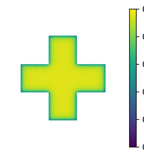
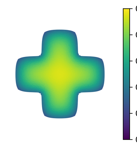
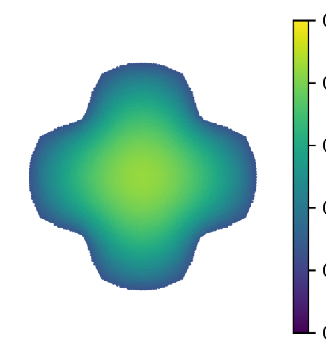
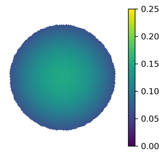
Figure 2. Scatter plot of the particle positions at different times (from left to right, $t=0,0.05,0.2,8$) for the quadratic potential test case. The color scale refers to the density, computed for each particle as $m^{0}_{i}/|L_{i}|$.

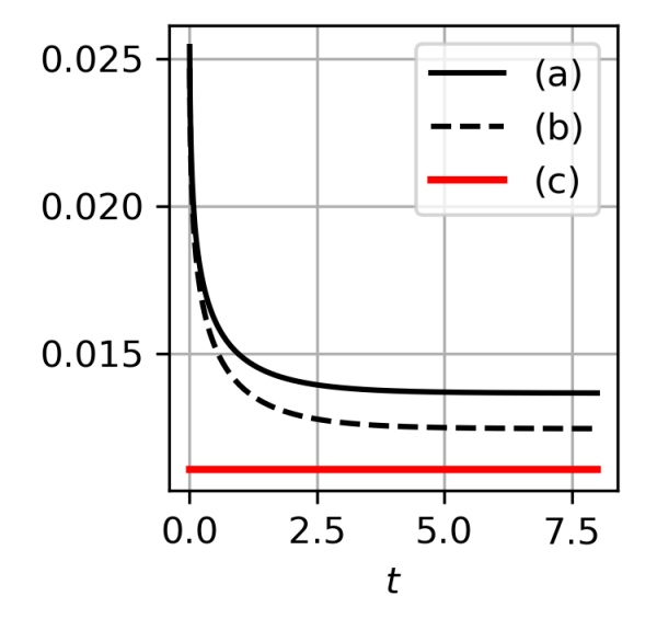
Figure 3. Energy evolution for the quadratic potential test case: (a) $F_{\varepsilon}(X)$; (b) $\sum_{i}U(m^{0}_{i}/|L_{i}|)|L_{i}|$; (c) internal energy of the equilibrium density $\int U(\rho_{\infty})$.

Appendix A Optimal transport tools and proof of Proposition 2.3

A.1. Optimal transport

Given two positive measures $\rho,\mu\in\mathcal{M}_{+}(\Omega)$ with fixed total mass $\rho[\Omega]=\mu[\Omega]$, the $L^{2}$-Wasserstein distance between $\rho$ and $\mu$, is defined via the following minimization problem

(A.1) $$W^{2}_{2}(\rho,\mu)=\min\left\{\int_{\Omega\times\Omega}|x-y|^{2}\mathrm{d}\gamma(x,y)\,;\quad\gamma\in\Pi(\rho,\mu)\right\}$$

where $\Pi(\rho,\mu)$ is the set of coupling plans $\gamma\in\mathcal{M}_{+}(\Omega\times\Omega)$ verifying

$$\int_{\Omega\times\Omega}\psi(x)\mathrm{d}\gamma(x,y)=\int_{\Omega}\psi(x)\mathrm{d}\rho(x)\,,\quad\int_{\Omega\times\Omega}\psi(y)\mathrm{d}\gamma(x,y)=\int_{\Omega}\psi(y)\mathrm{d}\mu(y)\,,$$

for all functions $\psi\in C(\Omega)$. Problem (A.1) always admits at least a solution $\gamma$, and we call this optimal transport plan from $\rho$ to $\mu$.

Semi-discrete optimal transport refers to the case one of the two measures is discrete and the other is absolutely continuous. In this case, it can be shown that (A.1) admits a dual formulation which can be expressed in terms of Laguerre tessellations. Suppose that $\mu=\sum_{i}m_{i}\delta_{x_{i}}$ where $X=(x_{i})_{i}\in(\mathbb{R}^{d})^{N}$ and $m_{i}>0$, and that $\rho\in\mathcal{M}_{+}(\Omega)$ is absolutely continuous and satisfies $\rho[\Omega]=\sum_{i}m_{i}$, then

(A.2) $$W^{2}_{2}(\rho,\mu)=\max_{w\in\mathbb{R}^{N}}\sum_{i}\left(\int_{L_{i}(X,w)}\left(|x-x_{i}|^{2}-w_{i}\right)\mathrm{d}\rho(x)+w_{i}m_{i}\right).$$

The maximum is always attained and the maximizer $w\in\mathbb{R}^{N}$ is related to the optimal plan $\gamma$ by

$$\int_{\Omega\times\Omega}\psi(x,y)\mathrm{d}\gamma(x,y)=\sum_{i}\int_{L_{i}(X,w)}\psi(x,x_{i})\mathrm{d}\rho(x)\,\quad\forall\,\psi\in C(\Omega\times\Omega)\,.$$

A.2. Energy reformulation

Let us show the equivalence between (1.1) and (1.10). Suppose that $X\in\mathbb{R}^{d}\setminus\Delta_{N}$. Then, by definition of the $W_{2}$ distance,

(A.3) $$F_{\varepsilon}(X)\geq\inf_{a\in\mathbb{R}^{N}_{>0},\eta\in\mathcal{C}}\frac{W_{2}^{2}\Big{(}\sum_{i}a_{i}\delta_{x_{i}},\eta\Big{)}}{2\varepsilon}+\sum_{i}C_{i}(a_{i})\eqqcolon E_{\varepsilon}(X)$$

where $F_{\varepsilon}(X)$ is given by (1.1), and where $\mathcal{C}=\{{\mathrm{d}x}\}$ if $\mathbb{L}_{N}(\Omega)=\mathbb{T}_{N}(\Omega)$, and $\mathcal{C}=\{f\mathrm{d}x\,:\,f:\Omega\rightarrow[0,1]\}$ if $\mathbb{L}_{N}(\Omega)=\mathbb{T}_{N}^{s}(\Omega)$. Note that the minimization on the right hand side of (A.3) is implicitely taken under the constraint $\sum_{i}a_{i}=\eta[\Omega]$, and we will keep using this convention in the following. Using the dual formulation (A.2) and exchanging inf and sup we find

$$E_{\varepsilon}(X)\geq\sup_{w\in\mathbb{R}^{N}}\inf_{a\in\mathbb{R}^{N}_{>0},\eta\in\mathcal{C}}\sum_{i}\left(\int_{L_{i}(X,w)}\frac{|x-x_{i}|^{2}-w_{i}}{2\varepsilon}\mathrm{d}\eta(x)+\frac{w_{i}}{2\varepsilon}a_{i}+C_{i}(a_{i})\right)$$

Optimizing over $\eta$ and $a$, we find that the right-hand side is equal to $D_{\varepsilon}(X)=F_{\varepsilon}(X)$ and thereofore $F_{\varepsilon}(X)=E_{\varepsilon}(X)$.

A.3. Proof of Proposition 2.3

Let $X,Y\in(\mathbb{R}^{d})^{N}\setminus\Delta_{N}$ and $\mathcal{L}\in\mathbb{L}_{N}(\Omega)$ the optimal tessellation associated with $X$. Then

$$F_{\varepsilon}(Y) \leq\sum_{i}\int_{L_{i}}\frac{|x-x_{i}+x_{i}-y_{i}|^{2}}{2\varepsilon}+C(|L_{i}|)$$

$$\leq F_{\varepsilon}(X)+\langle G_{\varepsilon}(X),Y-X\rangle_{m^{0}}+|\Omega|\sum_{i}\frac{|x_{i}-y_{i}|^{2}}{2\varepsilon}\,,$$

where

$$(G_{\varepsilon}(X))_{i}\coloneqq\frac{|L_{i}|}{m^{0}_{i}}\frac{x_{i}-b_{i}}{\varepsilon}\,,\quad b_{i}\coloneqq\frac{1}{|L_{i}|}\int_{L_{i}}x\,\mathrm{d}x\,.$$

This shows that $G_{\varepsilon}(X)\in\partial^{+}F_{\varepsilon}(X)$, the Fréchet superdifferential of $F_{\varepsilon}$ at $X$. We now prove that $G_{\varepsilon}(X)$ is continuous, which is implies that $F_{\varepsilon}(X)$ is $C^{1}$ and that $G_{\varepsilon}(X)$ is its gradient at $x$ with respect to the inner product $\langle\cdot,\cdot\rangle_{m^{0}}$. For this, we will use the following expression for $F_{\varepsilon}(X)$ (shown in Section A.2):

(A.4) $$F_{\varepsilon}(X)=\min_{a\in\mathbb{R}^{N},\eta\in\mathcal{C}}\frac{W^{2}_{2}(\eta,\sum_{i}a_{i}\delta_{x_{i}})}{2\varepsilon}+\sum_{i}C_{i}(a_{i})$$

where $\mathcal{C}$ is a convex subset of $\mathcal{M}(\Omega)$ defined as above. If $X\in(\mathbb{R}^{d})^{N}\setminus\Delta_{N}$, then problem (A.4) admits a unique solution which is linked to the solution $\mathcal{L}(X)=\{L_{i}(X)\}_{i}$ of problem (1.1) by

$$\eta(X)=\sum_{i}\boldsymbol{1}_{L_{i}(X)}\mathrm{d}x\,,\quad a_{i}(X)=|L_{i}(X)|\,.$$

Since the function minimized in (A.4) is continuous with respect to $a$ and $\eta$ (with respect to the narrow topology) on the set $\{(a,\eta)\,:\,\sum_{i}a_{i}=\eta[\Omega]\}$, then the optimal $\eta(X)$ and $a_{i}(X)$ are continuous functions of $X$ on $(\mathbb{R}^{d})^{N}\setminus\Delta_{N}$. In particular, given a sequence $(X^{n})_{n}\subset(\mathbb{R}^{d})^{N}\setminus\Delta_{N}$, such that $X^{n}=(x^{n}_{i})_{i}\rightarrow X\in(\mathbb{R}^{d})^{N}\setminus\Delta_{N}$ for $n\rightarrow\infty$, we have

$$\eta(X^{n})\rightharpoonup\eta(X)\,,\quad\sum_{i}a_{i}(X^{n})\delta_{x^{n}_{i}}\rightharpoonup\sum_{i}a_{i}(X)\delta_{x_{i}}\,.$$

Denoting by $\gamma^{n}\in\mathcal{M}(\mathbb{R}^{d},\mathbb{R}^{d})$ the optimal transport plan from $\eta(X^{n})$ to $\sum_{i}a_{i}(X^{n})\delta_{x^{n}_{i}}$, by the stability of optimal transport plans $\gamma^{n}\rightharpoonup\gamma$, the optimal plan from $\eta(X)$ to $\sum_{i}a_{i}(X)\delta_{x}$. Now, for any $\varepsilon>0$ and $n$ sufficiently large we can assume that $|x^{n}_{i}-x^{n}_{j}|\geq 3\varepsilon$ for all $i\neq j$, and $|x_{i}-x^{n}_{i}|\leq\varepsilon$. Then let $B(x_{i},\delta)$ the closed ball of radius $\delta>0$ centered at $x_{i}$, and consider a continuous function $\psi:\mathbb{R}^{d}\rightarrow\mathbb{R}$ such that $\psi(x)=1$ for $x\in B(x_{i},\varepsilon)$, and $\psi(x)=0$ for $x\in\mathbb{R}^{d}\setminus B(x_{i},2\varepsilon)$. Then, for $n\rightarrow+\infty$,

$$\int_{L_{i}(X^{n})}x\mathrm{d}x=\int_{\mathbb{R}^{d}\times\mathbb{R}^{d}}x\psi(y)\mathrm{d}\gamma^{n}(x,y)\rightarrow\int_{\mathbb{R}^{d}\times\mathbb{R}^{d}}x\psi(y)\mathrm{d}\gamma(x,y)=\int_{L_{i}(X)}x\mathrm{d}x\,,$$

which shows that $G_{\varepsilon}(X)$ is continuous.

References

- [1] Wolfgang Alt. Nonlinear hyperbolic systems of generalized Navier-Stokes type for interactive motion in biology. In Geometric Analysis and Nonlinear Partial Differential Equations, pages 431–461. Springer, 2003.
- [2] Jean-David Benamou, Guillaume Carlier, Quentin Mérigot, and Edouard Oudet. Discretization of functionals involving the Monge–Ampère operator. Numerische mathematik, 134(3):611–636, 2016.
- [3] Yann Brenier. Derivation of the Euler Equations from a Caricature of Coulomb Interaction. Communications in Mathematical Physics, 212(1):93–104, 2000.
- [4] Jose A Carrillo, Daniel Matthes, and Marie-Therese Wolfram. Lagrangian schemes for Wasserstein gradient flows. Handbook of Numerical Analysis, 22:271–311, 2021.
- [5] José Antonio Carrillo, Yanghong Huang, Francesco Saverio Patacchini, and Gershon Wolansky. Numerical study of a particle method for gradient flows. Kinetic and Related Models, 10(3):613–641, 2017.
- [6] Constantine M Dafermos, Constantine M Dafermos, Constantine M Dafermos, Grèce Mathématicien, Constantine M Dafermos, and Greece Mathematician. Hyperbolic conservation laws in continuum physics, volume 3. Springer, 2005.
- [7] Lawrence C Evans, Ovidiu Savin, and Wilfrid Gangbo. Diffeomorphisms and nonlinear heat flows. SIAM journal on mathematical analysis, 37(3):737–751, 2005.
- [8] John A Fozard, Helen M Byrne, Oliver E Jensen, and Julie R King. Continuum approximations of individual-based models for epithelial monolayers. Mathematical medicine and biology: a journal of the IMA, 27(1):39–74, 2010.
- [9] Thomas O Gallouët and Quentin Mérigot. A Lagrangian scheme à la Brenier for the incompressible Euler equations. Foundations of Computational Mathematics, 18(4):835–865, 2018.
- [10] Thomas O Gallouët, Quentin Merigot, and Andrea Natale. Convergence of a Lagrangian discretization for barotropic fluids and porous media flow. SIAM Journal on Mathematical Analysis, 54(3):2990–3018, 2022.
- [11] Jan Giesselmann, Corrado Lattanzio, and Athanasios E Tzavaras. Relative energy for the Korteweg theory and related Hamiltonian flows in gas dynamics. Archive for Rational Mechanics and Analysis, 223(3):1427–1484, 2017.
- [12] Darryl D Holm, Jerrold E Marsden, and Tudor S Ratiu. The Euler–Poincaré equations and semidirect products with applications to continuum theories. Advances in Mathematics, 137(1):1–81, 1998.
- [13] Hisao Honda. Geometrical models for cells in tissues. International review of cytology, 81:191–248, 1983.
- [14] Gareth Wyn Jones and S Jonathan Chapman. Modeling growth in biological materials. Siam review, 54(1):52–118, 2012.
- [15] Boris Khesin, Gerard Misiołek, and Klas Modin. Geometric hydrodynamics and infinite-dimensional Newton’s equations. Bulletin of the American Mathematical Society, 58(3):377–442, 2021.
- [16] Jun Kitagawa, Quentin Mérigot, and Boris Thibert. Convergence of a Newton algorithm for semi-discrete optimal transport. Journal of the European Mathematical Society, 21(9):2603–2651, 2019.
- [17] Hugo Leclerc, Quentin Mérigot, Filippo Santambrogio, and Federico Stra. Lagrangian discretization of crowd motion and linear diffusion. SIAM Journal on Numerical Analysis, 58(4):2093–2118, 2020.
- [18] Yang Liu, Wenping Wang, Bruno Lévy, Feng Sun, Dong-Ming Yan, Lin Lu, and Chenglei Yang. On centroidal Voronoi tessellation—energy smoothness and fast computation. ACM Transactions on Graphics (ToG), 28(4):1–17, 2009.
- [19] Stuart Lloyd. Least squares quantization in PCM. IEEE transactions on information theory, 28(2):129–137, 1982.
- [20] Quentin Mérigot and Jean-Marie Mirebeau. Minimal geodesics along volume-preserving maps, through semidiscrete optimal transport. SIAM Journal on Numerical Analysis, 54(6):3465–3492, 2016.
- [21] Quentin Mérigot, Filippo Santambrogio, and Clément Sarrazin. Non-asymptotic convergence bounds for Wasserstein approximation using point clouds. Advances in Neural Information Processing Systems, 34:12810–12821, 2021.
- [22] Quentin Merigot and Boris Thibert. Optimal transport: discretization and algorithms. In Handbook of Numerical Analysis, volume 22, pages 133–212. Elsevier, 2021.
- [23] Felix Otto. The geometry of dissipative evolution equations: The porous medium equation. Communications in Partial Differential Equations, 26(1-2):101–174, 2001.
- [24] C Ruscher, J Baschnagel, and J Farago. The voronoi liquid. EPL (Europhysics Letters), 112(6):66003, 2016.
- [25] Clément Sarrazin. Lagrangian discretization of variational mean field games. SIAM Journal on Control and Optimization, 60(3):1365–1392, 2022.
- [26] Ronald Votel, David AW Barton, Takahide Gotou, Takeshi Hatanaka, Masayuki Fujita, and Jeff Moehlis. Equilibrium configurations for a territorial model. SIAM Journal on Applied Dynamical Systems, 8(3):1234–1260, 2009.