Sensitivity analysis for ReaxFF reparameterization using the Hilbert–Schmidt independence criterion

Abstract

We apply a global sensitivity method, the Hilbert–Schmidt independence criterion (HSIC), to the reparameterization of a Zn/S/H ReaxFF force field to identify the most appropriate parameters for reparameterization. Parameter selection remains a challenge in this context as high dimensional optimizations are prone to overfitting and take a long time, but selecting too few parameters leads to poor quality force fields. We show that the HSIC correctly and quickly identifies the most sensitive parameters, and that optimizations done using a small number of sensitive parameters outperform those done using a higher dimensional reasonable-user parameter selection. Optimizations using only sensitive parameters: 1) converge faster, 2) have loss values comparable to those found with the naive selection, 3) have similar accuracy in validation tests, and 4) do not suffer from problems of overfitting. We demonstrate that an HSIC global sensitivity is a cheap optimization pre-processing step that has both qualitative and quantitative benefits which can substantially simplify and speedup ReaxFF reparameterizations.

Ghent University]Center for Molecular Modeling, Ghent University, Ghent, Belgium Software for Chemistry and Materials BV, Amsterdam, the Netherlands Ghent University]Center for Molecular Modeling, Ghent University, Ghent, Belgium

1 Introduction

1.1 ReaxFF reparameterization

The ReaxFF (reactive force field) ^{1, 2} is a potential energy surface (PES) for modelling reactive chemistry at spatial and temporal scales typically unreachable with other, more accurate, but expensive methods. ReaxFF’s speed comes at the cost of replacing accurate formalism with empirical equations that can typically contain hundreds of fitted parameters. Many of these parameters have no easy physical interpretability and only expert users may have a notion of appropriate values.

This makes the task of fixing the parameters quite difficult. The procedure typically used to do this is the minimization of some cost function which measures the deviations between predictions made by ReaxFF and some training set of values the user would like to replicate ^{3, 4, 5, 6, 7, 8, 9, 10, 11, 12}. However, the question of which parameters should be optimized has always been a difficult one. Optimizing all potentially relevant parameters simultaneously is prone to producing overfitted results, and very high dimensional optimizations are costly and insufficiently exploratory ⁴. A key conclusion from our previous work ^{4, 13} is that the careful conditioning of the error function (in terms of parameter selection and training set items) is crucial to obtaining reasonable results.

Typically, researchers apply rudimentary sensitivity analyses and expert knowledge to guide parameter selection. However, these processes are usually inaccurate, laborious, or do not sample the space sufficiently. In this work, we aim to address this problem by introducing a systematic global sensitivity analysis technique to guide parameter selection in a more robust manner. This method has also been coded into our ParAMS package ¹⁴, making it a seamless part of any reparameterization workflow.

1.2 Global sensitivity methods

Uncertainty analysis concerns itself with the propagation of uncertainty from a model’s inputs to its outputs, i.e., estimating an outputs’ distribution given all possible changes in the inputs ¹⁵. Sensitivity analysis attributes the uncertainty of the outputs to particular inputs. This is broadly done by measuring how much the unconditioned output distribution, $\mathbb{P}(Y)$, differs from the output distribution given certain inputs, $\mathbb{P}(Y|X_{i})$ ^{16, 17}. The type of statistical operator used to make this comparison divides global sensitivity methods into two types; variance-based and distribution-based.

Variance-based methods assume that the variances of these distributions are sufficient to describe them ^{16, 18}. This approach is well-established, and the first we tried. One of the most popular variance-based techniques is known as the Sobol method. It is based on the assumption that the total variance on the outcomes of a model $Y$ can be linearly apportioned to every input and combination of inputs ¹⁹:

$$\sum_{i}S_{i}+\sum_{i}\sum_{j>i}S_{ij}+\sum_{i}\sum_{j>i}\sum_{k>j}S_{ijk}+\dots+S_{123\dots d}=1.$$ (1)

$S_{i}$ is the Sobol index for the first order effect of parameter $i$ calculated as ¹⁹:

$$S_{i}=\frac{\mathbb{V}(\mathbb{E}(Y|X_{i}))}{\mathbb{V}(Y)},$$ (2)

where $\mathbb{E}$ and $\mathbb{V}$ indicate the expected value and variance respectively. Higher-order effects are calculated similarly:

$$S_{ij}=\frac{\mathbb{V}(\mathbb{E}(Y|X_{i},X_{j}))}{\mathbb{V}(Y)}.$$ (3)

A special case is known as the total effect, and is calculated as:

$$S_{Ti}=1-\frac{\mathbb{V}(\mathbb{E}(Y|\mathbf{X}_{-i}))}{\mathbb{V}(Y)},$$ (4)

where $\mathbf{X}_{-i}$ denotes the vector of all parameters except $X_{i}$. A full decomposition of the variance is prohibitive for all but the smallest number of dimensions since a total of $2^{d}-1$ indices need to be calculated. It has, however, been shown that the first effect and total effect are sufficient for identifying the most sensitive parameters ¹⁹.

The main disadvantage of this method is its cost in terms of the number of samples needed. An efficient method to calculate the first and total effect Sobol indices requires $\eta(d+2)$ function evaluations ¹⁹. There is no prescribed way to select $\eta$, but it is typically on the order of several thousand ^{20, 21}. Since the cost of the calculation of the indices themselves is trivial in comparison to the cost of obtaining the samples, the recommended procedure in literature is to iteratively sample and calculate until the indices converge. In this work, we attempt to introduce a preprocessing step to a ReaxFF parameterization, and thus the cost of this should be significantly less than the optimization; literature sources suggest that this will not be the case ^{21, 20}.

The intractable expense of the Sobol method is well-known, and much effort has gone into decreasing its cost ¹⁹. One popular method which is significantly cheaper than the Sobol one, is the elementary effects method, also known as Morris screening ²². Morris screening uses a careful sampling strategy to calculate an ‘estimated effect’ which has been shown to be a good proxy for the total effect Sobol index ^{19, 22}. This method is a popular screening method for dimensionality reduction in literature, particularly for expensive models. In theory, Morris screening should be a suitable method for our purposes, however, in our early investigations, this proved to not be the case.

Both Sobol indices and Morris screening impose rules on how samples may be generated. In the case of Sobol indices, certain parameter values must be fixed while allowing others to vary. In the case of Morris screening, samples are gathered in trajectories where individual parameters are changed one at a time. In our particular context, these rules make obtaining an adequate number of valid samples very frustrating and time-consuming. This is because the ReaxFF loss function surface is full of undefined points corresponding to parameter values which result in crashed calculations and nonphysical results. If such points are encountered when generating a Morris trajectory, for example, then the entire trajectory must be abandoned because these method do not allow the entry of nonfinite or undefined values. It would be simpler to find a method which allowed these values, or did not have sampling rules so that such instances could simply be discarded.

Aside from the real, practical issues related to their use, the assumptions made by variance-based techniques are inappropriate in the context of identifying parameter sensitivities in the ReaxFF error function. This is because it can produce extremely large values, and minima which are often located in narrow valleys and are unlikely to be captured during a sampling procedure ⁴. Cheaper approximation methods are typically insufficiently space-filling, or rely on strong assumptions about the structure of the inputs or outputs ^{23, 15}. The main criticism of variance-based techniques, however, is the fact that they limit the amount of information extracted from distributions to a single metric.

Distribution-based sensitivity approaches represent a newer family of methods. Unlike variance-based methods, these techniques do not reduce distributions to only their variance and can, in principle, capture arbitrary dependencies by considering the entirety of the distributions. Different statistics are used to measure the differences between distributions ¹⁶, and various methods of this type have been developed ^{18, 24, 23}. We are interested in the Hilbert–Schmidt Independence Criterion (HSIC) ²⁵ for it simplicity, speed and accuracy.

The HSIC was first introduced in Gretton et al. ²⁵. Through the use of kernels, it can identify arbitrary non-linear dependencies between the inputs and outputs ¹⁶. It is simpler and faster to converge than many other distribution-based techniques, and does not require explicit regularization ²⁵. It has since been used in: feature selection ^{26, 27, 24, 28, 29, 23}, event detection ^{30, 31}, machine learning ^{32, 33}, and dimensionality reduction in the context of global optimization ¹⁷, among other applications. This final use-case is of particular interest in our context and, other than Spagnol et al. ¹⁷, we have found no other work that directly applied the HSIC as a pre-optimization step.

In this work, we apply an HSIC analysis to a ReaxFF reparameterization problem. Based on the sensitivity results, we reduce the original high-dimensional optimization to a lower dimensional one. We then demonstrate that the optimization in this reduced space is able to produce ReaxFF force fields which are competitive with those produced by the higher dimensional optimization, but converge more quickly and reduce the risk of overfitting.

We focus on ReaxFF because parameterizations of this force field occur regularly in literature ^{34, 35, 10, 36, 37}. However, the techniques we introduce here could conceivably be applied to any high-dimensional parameterization problem of the type that occurs frequently in many fields ^{38, 39, 40, 41, 42, 43, 44, 45, 46}, because they all share the same underlying sloppy mathematical behavior ⁴⁷.

In the next section we will introduce ReaxFF, the HSIC metric, the kernels used, and the reparameterization loss function. In Section 4 we introduce a test case on which we apply the sensitivity technique, the results of which are described in Section 5, and future research paths are discussed in Section 6. Section 3 details our implementation of the calculation, and conclusions are drawn in Section 7.

2 Mathematical derivations

2.1 ReaxFF energy potential

The elucidation of the full ReaxFF energy potential is beyond the scope of this work, however, we provide a brief introduction here for context. Interested readers can consult Chenoweth et al. ⁵ and Senftle et al. ² for more details.

The ReaxFF energy potential is a summation of different energy contributions ⁵:

$$E_{\textrm{sys}}= E_{\textrm{bond}}+E_{\textrm{lp}}+E_{\textrm{over}}+E_{\textrm{under}}+E_{\textrm{val}}$$

$$+E_{\textrm{pen}}+E_{\textrm{coa}}+E_{\textrm{C2}}+E_{\textrm{triple}}$$

$$+E_{\textrm{tors}}+E_{\textrm{conj}}+E_{\textrm{H-bond}}+E_{\textrm{VdW}}$$

$$+E_{\textrm{charges}}+\dots$$ (5)

The main contribution is the bonding energy, $E_{\textrm{bond}}$, which calculates an energy based on bond orders, which are, in turn, calculated from atomic positions (the most fundamental inputs to any PES). The other contributions can be thought of as corrections to the bonding energy. Some corrections are general, for example $E_{\textrm{over}}$ and $E_{\textrm{under}}$ which penalize atoms which are over- or undercoordinated by their bonding. Some corrections are extremely specific, for example $E_{\textrm{C2}}$ which corrects the energy for the C₂ molecule. There is also an energy term for fluctuating charges ($E_{\textrm{charges}}$). ReaxFF typically uses either the EEM ⁴⁸ or ACKS2 ⁴⁹ charge models. In this work we use EEM charges.

Each of the energy contributions is typically a complicated function of bond orders and empirical parameters. For example ⁵:

$$E_{\textrm{bond}} =-D^{\sigma}_{e}\cdot BO^{\sigma}_{ij}\cdot\exp\left[p_{be1}\left(1-\left(BO^{\sigma}_{ij}\right)^{p_{be2}}\right)\right]$$

$$-D^{\pi}_{e}\cdot BO^{\pi}_{ij}-D^{\pi\pi}_{e}\cdot BO^{\pi\pi}_{ij}$$ (6)

where $D^{\sigma}_{e}$, $D^{\pi}_{e}$, $D^{\pi\pi}_{e}$, $p_{be1}$ and $p_{be2}$ are parameters and $BO_{ij}$ are bond orders.

The complexity and number of contributions quickly leads the ReaxFF PES to have a very large number of parameters, particularly because most parameters are a function of one or more atom types. For example, there is a $D^{\sigma}_{e}$ parameter for every combination of atom types being modelled.

In an effort to make the parameters easier to understand, the original authors organised them into the following groups or blocks: general, atoms, bonds, off-diagonal, angles, torsions and hydrogen bonds. These groups have no bearing on the calculation of the PES, but serve as a helpful organisational tool, and appear in the formatting rules for the inputs of most ReaxFF implementations. We will return to these groups when we introduce a new Zn/S/H force field in Section 4.1.

We use the term ‘force field’ in this work to refer to a full set of ReaxFF parameters and their values. Force fields are functions of the atom types they include and are sometimes only appropriate for specific conditions. For example, ReaxFF force fields containing hydrogen and oxygen are generally classed as appropriate for aqueous or combustion chemistry.

2.2 Loss function

The reparameterization of a force field requires the construction of a training set ($\mathbf{b}_{\text{ref}}\in\mathbb{R}^{m}$), which is a vector of $m$ scalar training point values of chemical properties that one would like ReaxFF to replicate. The goal of the reparameterization is the minimization of a loss function which quantifies the overall difference between the ReaxFF model and the training data in a single number. This loss function can take various forms, but the most common is the sum of square errors (SSE). We define the SSE as:

$$\mathrm{SSE}(\mathbf{x})\coloneqq\sum^{m}_{i=1}w_{i}\left(\frac{b_{\text{ref},i}-b(\mathbf{x},\mathbf{G}_{i})}{\sigma_{i}}\right)^{2}.$$ (7)

Each item in the training set ($b_{\text{ref},i}$) is compared to the result produced by the ReaxFF model ($b(\mathbf{x},\mathbf{G}_{i})$) using a vector of parameters which we allow to be adjusted ($\mathbf{x}$), and a set of system inputs and fixed parameters ($\mathbf{G}_{i}$). We will call the parameters we have chosen to optimize active parameters, and denote the set of active parameters $\mathscr{D}$. Items in the training set can be of different types (energies, forces, angles, etc.). To make them comparable and independent of units, each term in the loss function is divided by an appropriate $\sigma_{i}$ with the same unit as $b_{\text{ref},i}$. The $\sigma_{i}$ value is often understood as the acceptable error for that item. Finally, different training values can be weighted differently based on their importance via the weighting vector ($\mathbf{w}$). For example, it is more important to get energy minima correct than it is to replicate energies for very exaggerated geometries; one might weight the former higher than the latter in the loss function. In the case of multi-dimensional data, like forces, the $n\times 3$ matrix is simply flattened into the vector of training data. In other words, a single element of $\mathbf{b}_{\text{ref}}$ would not be ‘the forces on molecule A’ for example, but rather ‘the x-component of the forces on atom 1 in molecule A’. For more details regarding the implementation itself, readers are directed to the ParAMS documentation ¹⁴.

$\bm{\upsigma}$ and $\mathbf{w}$ perform essentially similar functions since they are both constants which could conceivably be combined. Using one, or the other, or both is a question of preference for different practitioners. Traditionally, only $\bm{\upsigma}$ was used, however for some users, weights provide a more intuitive value. We have chosen to use a fixed vector of values for $\bm{\upsigma}$, and adjust the weights to balance the training set.

2.3 Hilbert–Schmidt independence criterion

This section introduces the Hilbert–Schmidt independence criterion (HSIC) from a practitioner’s perspective. Our presentation is not as general as in other works, ^{25, 28, 17} and we only strive to explain the basic idea to readers interested in parameter selection. We will assume the space of a single parameter is $\mathcal{X}\subseteq\mathbb{R}$ and the space of loss values is $\mathcal{Y}\subseteq\mathbb{R}$. Typically, parameters are bounded and loss values are positive but these are not strict requirements for HSIC.

Let the Hilbert space of $\mathbb{R}$-valued functions on $\mathcal{X}$ be $\mathcal{H}_{x}:\mathcal{X}\rightarrow\mathbb{R}$, for which an inner product $\langle\cdot,\cdot\rangle_{\mathcal{H}_{x}}$ is defined. This is called a reproducing kernel Hilbert space (RKHS) when a kernel $k:\mathcal{X}\times\mathcal{X}\rightarrow\mathbb{R}$ exists such that $\forall x\in\mathcal{X}$ and $\forall f\in\mathcal{H}_{x}$:

$$k(x,\cdot) \in\mathcal{H}_{x}\text{ and }$$

$$\left\langle f,k(x,\cdot)\right\rangle_{\mathcal{H}_{x}} =f(x).$$

The second condition is known as the reproducing property: a function evaluation $f(x)$ can be reproduced by taking an inner product of $f$ with a partially evaluated kernel. We similarly define the RKHS, $\mathcal{H}_{y}$ with kernel $\ell$, for for the loss-value space $\mathcal{Y}$.

The kernel $k$ can be defined in terms of a feature map $\phi:\mathcal{X}\rightarrow\mathcal{F}_{x}$, where $\mathcal{F}_{x}$ is a new Hilbert space, often called the feature space of $x$. This means that each value $x$ is uniquely represented by a function $\phi(x)\in\mathcal{F}_{x}$. Any positive definite and symmetric kernel $k$ can always be described as an inner product in feature space:

$$k(x,x^{\prime}) \coloneqq\left\langle\phi(x),\phi(x^{\prime})\right\rangle_{\mathcal{F}_{x}}$$ (8)

In practice, direct use of $\phi$ is avoided and the kernel $k$ is used instead to keep calculations manageable. Kernels are generally cheap to evaluate, even when the feature map would be computationally infeasible. Similarly, a feature map $\psi:\mathcal{Y}\rightarrow\mathcal{F}_{y}$ exists, such that $\ell(y,y^{\prime})\coloneqq\left\langle\psi(y),\psi(y^{\prime})\right\rangle_{\mathcal{F}_{y}}$.

Now consider random variables $X\in\mathcal{X}$ and $Y\in\mathcal{Y}$, with a joint distribution $\mathbb{P}_{XY}$. Variance-based sensitivity methods characterize the dependence of $Y$ on $X$ with $\operatorname{cov}[X,Y]=\mathbb{E}_{XY}[XY]-\mathbb{E}_{X}[X]\mathbb{E}_{Y}[Y]$, which is only picking up linear correlations. In principle, one may overcome this limitation by computing the covariance in feature space instead: $\operatorname{cov}[\phi(X),\psi(Y)]=\mathbb{E}_{XY}[\phi(X)\psi(Y)]-\mathbb{E}_{X}[\phi(X)]\mathbb{E}_{Y}[\psi(Y)]$. However, the latter covariance is impractical because it directly operates in feature space and because the covariance is an element of a new Hilbert space $\mathcal{F}_{x}\otimes\mathcal{F}_{y}$, which troubles its direct interpretation. Gretton et al. ²⁵ showed how to overcome both issues by rewriting the squared norm of the latter covariance in terms of kernels:

$$\text{HSIC}(\mathcal{F}_{x},\mathcal{F}_{y},\mathbb{P}_{xy}) \coloneqq\bigl{\|}\operatorname{cov}[\phi(X),\psi(Y)]\bigr{\|}^{2}_{\mathcal{F}_{x}\otimes\mathcal{F}_{y}}$$ (9)

$$=\begin{aligned} &\mathbb{E}_{XX^{\prime}YY^{\prime}}[k(X,X^{\prime})\ell(Y,Y^{\prime})]\\ &+\mathbb{E}_{XX^{\prime}}[k(X,X^{\prime})]\mathbb{E}_{YY^{\prime}}[\ell(Y,Y^{\prime})]\\ &-2\mathbb{E}_{XY}\bigl{[}\mathbb{E}_{X^{\prime}}[k(X,X^{\prime})]\mathbb{E}_{Y^{\prime}}[\ell(Y,Y^{\prime})]\bigr{]}\end{aligned}$$ (10)

This definition of HSIC yields a positive real number, which increases as $X$ and $Y$ are more correlated. When $k$ and $\ell$ are linear kernels, HSIC reduces to $\bigl{|}\operatorname{cov}[X,Y]\bigr{|}^{2}$ and there is no added value compared to variance-based sensitivity criteria. In case of non-linear kernels, the HSIC also detects non-linear correlations between $X$ and $Y$. Ideally, $k$ and $\ell$ are characteristic kernels, ¹⁷ for which $\text{HSIC}=0$ if and only if $X$ and $Y$ are independent ($\mathbb{P}_{XY}=\mathbb{P}_{X}\mathbb{P}_{Y}$). Of the common kernels, the Gaussian kernel is characteristic, while the linear and polynomial kernels are not. It is possible to use non-characteristic kernels for HSIC, but then one loses the guarantee that all dependence will be captured ²⁸.

It is usually not possible to obtain $\mathbb{P}_{xy}$ explicitly, however, the HSIC can be estimated if we sample the distribution. We define a set of samples as:

$$Z\coloneqq(\mathbf{X},\mathbf{y}),$$ (11)

where $\mathbf{X}\in\mathbb{R}^{n\times d}$ is a matrix of $n$ rows of uniformly randomly sampled parameter vectors $\{\mathbf{X}_{1},\mathbf{X}_{2},\dots\mathbf{X}_{n}\}$, and we let $\mathbf{y}\in\mathbb{R}^{n}=\{\mathrm{SSE}(\mathbf{X}_{1}),\mathrm{SSE}(\mathbf{X}_{2})\dots,\mathrm{SSE}(\mathbf{X}_{n})\}$ be the corresponding set of loss function values.

To measure the sensitivity of a parameter with index $\omega$, we take the associated column with $n$ sample values, $\mathbf{X}_{\cdot\omega}$, and the loss values:

$$Z_{\omega}\coloneqq(\mathbf{X}_{\cdot\omega},\mathbf{y}),$$ (12)

and we make use of the unbiased estimator of the HSIC from Song et al. ²⁸:

$$\mathrm{HSIC}(\mathcal{F}_{x},\mathcal{F}_{y},Z_{\omega})\approx\frac{1}{n(n-3)}\left[\rho_{1}+\rho_{2}-\rho_{3}\right],$$ (13)

where:

$$\rho_{1} \coloneqq\mathrm{tr}(\mathbf{\tilde{K}}\mathbf{\tilde{L}})$$

$$\rho_{2} \coloneqq\frac{\bm{1}^{\top}\mathbf{\tilde{K}}\bm{1}\bm{1}^{\top}\mathbf{\tilde{L}}\bm{1}}{(n-1)(n-2)}$$

$$\rho_{3} \coloneqq\frac{2}{n-2}\bm{1}^{\top}\mathbf{\tilde{K}}\mathbf{\tilde{L}}\bm{1}$$

$$\mathbf{\tilde{K}}_{ij} \coloneqq(1-\delta_{ij})k(x_{i},x_{j})\quad\forall x_{i},x_{j}\in X_{\cdot\omega}$$

$$\mathbf{\tilde{L}}_{ij} \coloneqq(1-\delta_{ij})\ell(y_{i},y_{j})\quad\forall y_{i},y_{j}\in\mathbf{y}.$$

$\mathrm{HSIC}$ is a convenient metric with which to rank the influence of parameters on an output, however, to make interpretation even easier we define the sensitivity of a parameter as the normalized HSIC values ¹⁷:

$$s_{\omega}=\frac{\mathrm{HSIC}(\mathcal{F}_{x},\mathcal{F}_{y},Z_{\omega})}{\sum^{d}_{i=1}\mathrm{HSIC}(\mathcal{F}_{x},\mathcal{F}_{y},Z_{i})}.$$ (14)

By construction, sensitivity values are bounded ($0\leq s_{\omega}\leq 1$) and $\sum s_{\omega}=1$. This makes sensitivities a more intuitive value to interpret and understand than $\mathrm{HSIC}$.

The advantage of the biased HSIC estimator ²⁸ is that it is positive by construction. The unbiased estimator used here, although more accurate, runs the risk of producing small negative values for low sensitivity items. In the context of the sensitivity analysis, where a qualitative consideration of the results is arguably more important that a quantitative one, we simply clip any negative HSIC values to zero before calculating the sensitivities (Equation 14).

For a more detailed description of HSIC, the interested reader is directed to Gretton et al. ²⁵ for the original introduction, and to Da Veiga ²⁴, Song et al. ²⁸, De Lozzo and Marrel ²³ and Spagnol et al. ¹⁷ for more recent works.

Note that it is also possible to consider a more fine-grained sensitivity approach and let $\mathbf{y}$ be individual residual values (i.e., $y_{i}=b_{\text{ref},i}-b(\mathbf{x},\mathbf{G}_{i}))$. This would allow one to determine sensitivities for particular training set items; further information to assist in training set design. This represents an extension of the current work, and will not be dealt with here, but is left as an avenue for further study.

2.4 Kernels

Figure 1 illustrates the kernel distributions used in this work, using different parameter values where appropriate.

We select the characteristic Gaussian kernel for the parameters-kernel:

$$k(x,x^{\prime})\coloneqq\exp\left[-\frac{(x-x^{\prime})^{2}}{2\sigma^{2}}\right].$$ (15)

This captures the dis/similarity between parameters, and allows the distribution to take an arbitrary shape. For the sake of clarity, $\sigma$ as it is used in Equation 15 is unrelated to the same symbol in Equation 7.

We test several candidates for the loss-kernel. We first consider the non-characteristic threshold kernel introduced by Spagnol et al. ¹⁷:

$$\ell(y,y^{\prime}) \coloneqq h(y)h(y^{\prime})$$ (16)

$$h(y) \coloneqq\begin{cases}1&\text{ if }y<q_{\alpha},\\ 0&\text{ otherwise}.\end{cases}$$ (17)

$q_{\alpha}$ is the value corresponding to the $\alpha$ quantile of the data. The above kernel is constructed to focus the weight of the distribution on the smallest numerical values of $\mathbf{y}$ since these represent good loss function values we would like the most information about. Spagnol et al. ¹⁷ showed that thresholding was extremely important in identifying sensitivities near minima, and not allowing the calculation to be swamped by very large function values.

We then consider a characteristic and continuous approximation of the threshold kernel, which we call the conjunctive-Gaussian (CG) kernel:

$$\ell(y,y^{\prime})\coloneqq\exp\left[-\frac{(y^{2}+y^{\prime 2})}{2\gamma^{2}}\right],$$ (18)

where lower values of the $\gamma$ parameter focus the distribution more heavily on the best values.

For comparison, we also test a simple non-characteristic linear kernel:

$$\ell(y,y^{\prime})\coloneqq yy^{\prime},$$ (19)

and the Gaussian kernel introduced in Equation 15. Other kernels are possible, but we leave their consideration for later work.

To stabilize the numerics and handle order-of-magnitude concerns, we transform and scale the loss values before applying the loss-kernel to them:

$$\tilde{y}(y)=\frac{\ln{y}-\min{(\ln{\mathbf{y}})}}{\max{(\ln{\mathbf{y}})}-\min{(\ln{\mathbf{y}})}}.$$ (20)

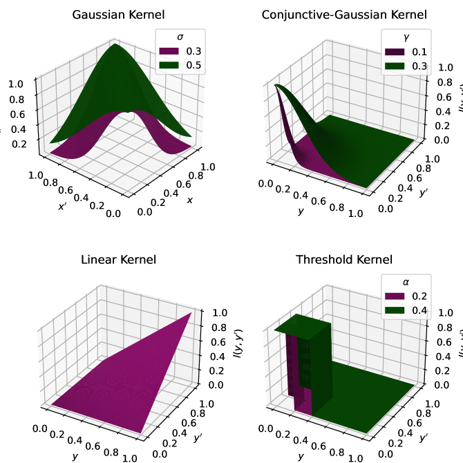
Figure 1: Plots of the tested kernel functions.

3 Software

Training data was calculated using the Amsterdam Modeling Suite (AMS) 2022.

The sensitivity calculation has been implemented in the Python programming language, and integrated into a development version of ParAMS 2023 ¹⁴, a reparameterization toolkit which comes bundled with AMS. It is also used to handle the force field optimizations through the GloMPO optimization management software ⁴.

4 The reparameterization problem

Our main goal in this work is to demonstrate the method and utility of our new sensitivity approach. For this reason, the training set we have designed is smaller than what would typically be required to create a production quality parameterization. Designing a large training set would require an entire publication in its own right, and distract heavily from the focus of our article. A smaller training set allows us to keep the discussions more focused and clear.

In any case, training set design is always an iterative process where more items are added as validation tests on the new force fields demonstrate deficiencies in the original set ⁵⁰. This work can be considered a first iteration upon which later work can build.

4.1 Initial force field

We aim to create a new ReaxFF force field which correctly models the adsorption of H2S on ZnS – an absorbent which has received some attention for its favorable electronic properties ^{51, 52, 53, 54, 55}. H2S is a common, but toxic, gas and its adsorption behavior on ZnS has been investigated for both gas detection ⁵⁵ and gas removal purposes ⁵³. As far as we are aware, however, no specially designed Zn/S/H ReaxFF force field exists to model this behaviour.

Table 1 details the nomenclature we will use to refer to the various parameter blocks which compose the ReaxFF force field file ⁵⁶. For a discussion of the parameter blocks, see Section 2.1

Table 1: Aliases used to refer to different parameter blocks in the ReaxFF force field file format.

Alias	Description	Number of parameters
GEN	General parameters	41
ATM:W	Parameters for atoms of type W	32 per atom type
BND:W.X	Parameters for W-X bonds	16 per W.X pair
OFD:W.X	Off-diagonal definitions for atom pairs	6 per W.X pair
ANG:W.X.Y	Parameters for angles formed by W-X-Y atoms	7 per angle group
TOR:W.X.Y.Z	Parameters for torsions formed by W-X-Y-Z atoms	7 per angle group
HBD:W.H.X	Hydrogen-bonding parameters for atoms W and X	4 per W.X pair

Our initial force field is an amalgamation of parameter values from already published force fields:

1. The ATM:S, BND:S.S and ANG:S.S.S parameter blocks are filled with values from the Li/S force field of Islam et al. ⁵⁷;

2. ATM:H, BND:S.H and ANG:H.S.H values are taken from the C/H/O/S force field of Müller and Hartke ⁵⁰;

3. GEN, ATM:Zn, BND:H.H, BND:Zn.H, BND:Zn.Zn, BND:Zn.S, ANG:Zn.Zn.S, ANG:Zn.S.Zn, ANG:Zn.S.S, ANG:S.Zn.S and HBD:S.H.S blocks are filled with parameters published in the Zn/O/H force field of Raymand et al. ⁵⁴. This force field does not contain any sulfur compounds, so the corresponding oxygen-related parameter blocks are used. For example, BND:Zn.O parameters are filled into the BND:Zn.S block of the initial force field.

The force field contains $279$ parameters. From this we use some common intuition – based on the contents of the training set and descriptions of the parameters – to select $53$ for initial optimization. The selection is ‘greedy’ in that a parameter is selected for optimization if:

1. it could conceivably affect the behaviour of a training set item,

2. the training set contains items related to the parameter, and

3. the parameter is appropriate for optimization.

For example, the atomic masses of the elements are technically parameters, however, changing them would not be appropriate. Similarly, $\pi$-bonds are not present in the training set, thus, their related parameters are not chosen for optimization. Finally, we do not optimize any atomic or general block parameters. These are generally known to be more ‘expert’ level parameters that are not suitable for preliminary stage optimization ¹⁴.

The $53$ parameters selected for optimization are listed in Table 2. The default parameter ranges supplied by ParAMS ¹⁴ were used, and can be found in the supplementary information.

Table 2: Initial naive parameter selection. Equation numbers and parameter names refer to notation used in ⁵⁸.

Block Name Eqn. Description Atoms ANG -p_hb2 18 Hydrogen bond/bond order H.S.H -p_hb3 18 Hydrogen bond parameter H.S.H p_hb1 2 Hydrogen bond energy H.S.H p_val1 13a Valance angle parameter H.S.H S.S.Zn S.Zn.S S.Zn.Zn Zn.S.Zn p_val2 13a Valance angle parameter H.S.H S.S.Zn S.Zn.S S.Zn.Zn Zn.S.Zn p_val4 13b Valance angle parameter H.S.H S.S.Zn S.Zn.S S.Zn.Zn Zn.S.Zn p_val7 13c Under-coordination H.S.H S.S.Zn S.Zn.S S.Zn.Zn Zn.S.Zn Theta_0,0 13g 180°-(equilibrium angle) H.S.H S.S.Zn S.Zn.S S.Zn.Zn Zn.S.Zn HBD r_hb^0 18 Hydrogen bond equilibrium distance S.H.S BND D_e^sigma 6, 11a Sigma-bond dissociation energy H.S S.S S.Zn Zn.Zn p_be1 6 Bond energy parameter H.S S.S S.Zn Zn.Zn p_be2 6 Bond energy parameter H.S S.S S.Zn Zn.Zn p_bo1 2 Sigma bond order H.S S.S S.Zn Zn.Zn p_bo2 2 Sigma bond order H.S S.S S.Zn Zn.Zn p_ovun1 11a Over-coordination penalty H.S S.S S.Zn Zn.Zn

4.2 Training data

The training set, calculated with BAND using PBEsol and DZ or DZP basis set, consists of 16 jobs, from which 471 individual training points are extracted.

AMS BAND calculates charges via the Hirshfeld, Voronoi deformation, Mulliken and CM5 methods. We have included Hirshfeld charges in our training set. Although these charges are not without problems ⁵⁹, we believe they are the best available. The accuracy of these charges is also not overly important since we do not activate any charge related parameters in our initial parameter selection (see Section 4.1), and the few charges we include in the training set are mainly used as a sanity check on the results.

The training set consists of:

1. energy-volume scans, charges and enthalpies of formation for the cubic zincblende, cubic rocksalt and hexagonal wurtzite structures of ZnS;

2. the optimized geometry, charges, H-S bond scan, and H-S-H angle scan for H2S;

3. the energy of formation, bond lengths, charges, and angles of a periodic zincblende surface;

4. the forces of a distorted zincblende surface;

5. the charges, bond length and adsorption energy of H2S adsorbed on zincblende.

Details of the training set are included in Section F of the supplementary information.

Default ParAMS values are used for $\bm{\upsigma}$. Individual energies, angles, distances, charges and torsions, and force groups are equally weighted in the initial training set. The full training set, job collection and initial parameter interface are available in the supplementary information.

5 Results and discussion

Our workflow proceeds as follows:

reparameterization of the initial force field

based on the naive parameter selection (done purely for comparative purposes);

running of the sensitivity calculation

to determine a parameter ordering (entirely independent of the previous step);

rerunning the reparameterization

using 10, 20, 33 and 43 of the least and most sensitive parameters, as determined by the sensitivity analysis;

running validation tests

using the initial parameterization and some of the best parameterizations found.

Our aim is to show that:

1. the HSIC sensitivity method correctly identifies the most sensitive parameters;

2. reparameterizations within a lower dimensional space of very sensitive parameters can find force fields of similar quality in a shorter amount of time;

3. reparameterizations in higher dimension run the risk of overfitting.

5.1 Initial optimizations

An initial set of sixteen reparameterizations were performed using the Covariance Matrix Adaptation - Evolutionary Strategy (CMA-ES) ⁶⁰ which has been shown to work well on ReaxFF reparameterizations ^{13, 4}. All the optimizers were started from the initial force field values described in Section 4.1 with a wide initial sampling distribution ($\sigma_{0}=0.5$). All parameters were scaled between zero and one according to their bounds which are automatically suggested by ParAMS.

Optimizers were stopped if:

1. within the last $2000$ function evaluations their lowest value had not improved, and their explored values were very similar; or

2. any of the default internal CMA-ES convergence criteria were triggered.

The optimizers were run in parallel and the entire optimization was stopped after using a cumulative total of $300\,000$ function evaluations. These conditions are all quite strict and provided all the optimizers a very long time to find the best possible minimum.

Figure 2 shows the optimizer trajectories for these reparameterizations, and shows the original loss of $20\,662$ being improved to between $410$ and $308$. These results will be discussed in more detail in Section 5.3 when comparing the results to other optimizations. Detailed results for every optimizer can be found in the Section A of the supplementary information.

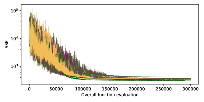
Figure 2: Optimizer trajectories for the sixteen CMA-ES reparameterizations of the initial force field using the naive parameter selection.

5.2 Sensitivity analysis

A total of $10\,000$ uniformly randomly generated samples of the original optimization space were collected for the sensitivity analysis. The sampling procedure took a total of $142\text{\,}\mathrm{min}$ on a $64$ core node (AMD EPYC $7513$ @ $2.6\text{\,}\mathrm{GHz}$). This sampling took place once, and this same set of samples was used in all the sensitivity calculations.

The distribution of sampled loss values (and their transformed values, $\tilde{y}$) is shown in Figure 3; the lowest value is $2651$. Approximately half of the samples are actually worse than the initial loss value, and the set clearly does not include the good minima found through the original optimizations in Section 5.1. We will demonstrate that having such minima in the sample set is not a requirement for having a good estimation of parameter sensitivity.

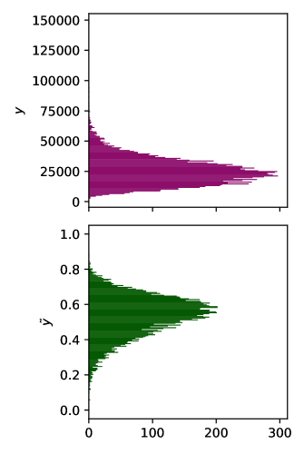
Figure 3: Distribution of loss values (top), and loss values scaled according to Equation 20 (bottom), gathered during the sampling procedure and used during the sensitivity analyses.

Instead of using all of the samples at once in a single HSIC calculation, we repeated it $10$ times using a bootstrapping method. Each bootstrap used $2000$ random sub-samples from the original $10\,000$ sample set. Using fewer samples per calculation significantly speeds up calculation time, and the spread of the results gives us an indication of the error. Unless otherwise mentioned, the sensitivity values discussed below refer to the average value across the $10$ repeats. Algorithm 1 provides a pseudocode of the calculation where we have abandoned notational precision for brevity and clarity.

Algorithm 1 Sensitivity calculation workflow.

SSE, $k$, $\ell$

1:randomly generate $\mathbf{X}\in\mathbb{R}^{$10\,000$\times 53}$

2:$\mathbf{y}\in\mathbb{R}^{$10\,000$}\leftarrow\mathrm{SSE}(\mathbf{X})$ $\triangleright$ Evaluate loss

3:$\tilde{\mathbf{y}}\leftarrow\tilde{y}(\mathbf{y})$ $\triangleright$ Scale loss values $i=1,\dots,10$ $\triangleright$ Repeat the calculation

4:$\mathbf{X}^{\mathrm{sub}}\leftarrow$ $2000$ random rows of $\mathbf{X}$

5:$\tilde{\mathbf{y}}^{\mathrm{sub}}\leftarrow$ corresponding $2000$ loss values

6:$\tilde{\mathbf{L}}\leftarrow\ell(\tilde{\mathbf{y}}^{\mathrm{sub}})$ $\omega=1,\dots,53$ $\triangleright$ Every parameter

7:$\tilde{\mathbf{K}}\leftarrow k(\mathbf{X}^{\mathrm{sub}}_{\cdot\omega})$

8:$\mathbf{H}_{i\omega}\leftarrow\mathrm{HSIC}(\tilde{\mathbf{K}},\tilde{\mathbf{L}})$

9:$\mathbf{h}\leftarrow$ Mean$\mathbf{H}_{1},\dots,\mathbf{H}_{10}$ $\triangleright$ Average repeats

10:$s_{j}\leftarrow\frac{h_{j}}{\sum_{i}h_{i}}$ $\triangleright$ Calculate sensitivities

The following kernels were applied to the loss values: CG kernel ($\gamma=0.3$), Gaussian kernel ($\sigma=0.3$), linear kernel and threshold kernel ($\alpha=0.4$). In all cases a Gaussian kernel ($\sigma=0.3$) was applied to parameter values. Since all values are scaled between 0 and 1, a value of $\sigma=0.3$ approximates the median distance between all samples in a uniform distribution between these values. This has repeatedly been reported as an appropriate value ^{61, 17}.

The average time needed to perform the sensitivity calculation (regardless of loss-kernel and including the repeats) was approximately $60\text{\,}\mathrm{s}$. The optimizations require several days to complete, thus the inclusion of these sampling and sensitivity steps in a reparameterization workflow would not be the limiting step and, as will be shown below, come with several advantages.

We note that we also repeated the calculations using a sample pool of $30\,000$ samples, and $10\,000$ sub-samples per calculation. These results produce tighter distributions between the repeats at the cost of more time, but the average sensitivity values are essentially the same. In other words, they were not worth the effort and are not presented below.

The scaling of the sensitivity calculation is $\mathcal{O}(rdn^{2})$ where $r$ are the number of repeats, $d$ is the number of parameters, and $n$ is the number of sub-samples used per calculation. Increasing the size of the matrices has the largest impact on the calculation time, so being able to get robust parameter orderings from repeated calculations using small sub-samples is very advantageous.

Figure 4 compares the sensitivity values determined by each calculation for each parameter. Despite the large differences between loss-kernels, the ordering of parameters is very robust for the most sensitive parameters. Significant deviations only appear for the least sensitive parameters which are all close to one another numerically (note the logarithmic axis). This demonstrates that the HSIC approach we have taken is robust, and not overly dependent on the choice of loss-kernel or hyperparameters.

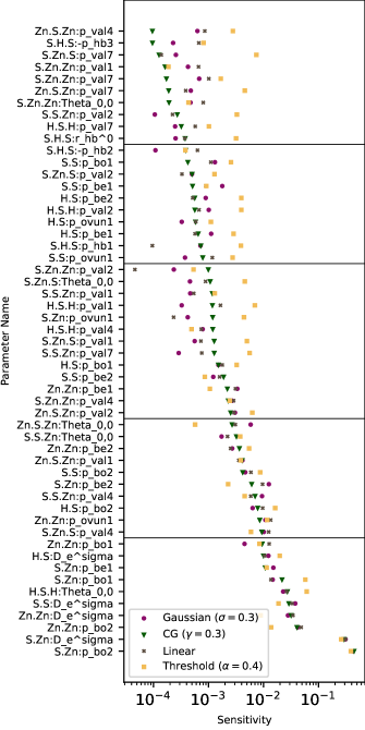
Figure 4: Average sensitivity values (over ten runs each) determined for each parameter using different kernels applied to the loss values. Parameters are ordered by the results of the CG kernel which is used in the later reparameterizations. Black lines group the $10203343$ most sensitive parameters.

The loss-kernel which struggles the most with differentiating sensitivities is the threshold kernel. We believe that this is because the kernel is discontinuous and provides very little information to the calculation because values are toggled to zero or one. Our investigation of this kernel was motivated by the work of Spagnol et al. ¹⁷. They demonstrated the necessity of this kernel to focus the calculation on small loss values (near the minima of interest), and negate the effects of large order-of-magnitude differences. As discussed in Section 2.4, our implementation always takes the logarithm of the loss values and then scales the result; it appears to address the order-of-magnitude problem. Random sampling will also generally not contain very good minima (true in this case, as discussed above), making the second advantage of the threshold kernel less important. The continuity provided by the other kernels seems to make converging the sensitivity values for the parameters easier.

We have also explored the effect of using different kernel parameters in Section B of the supplementary information. This has a minor effect on the sensitivity results, provided a reasonable kernel parameter value is selected so that the kernel values are not all very close to zero or one.

Given the similarities in orderings obtained by the various loss-kernels we will continue discussing only the results obtained when using the CG kernel ($\gamma=0.3$). This is a somewhat arbitrary choice, but it can be argued that it has the best theoretical foundation by emphasizing the sensitivities for low minima.

Figure 5 shows the sensitivities obtained grouped by a) parameter group, and b) parameter name. For example, ‘S.Zn’ refers to all the bond parameters associated with sulphur-zinc bonds, and p_bo2 refers to all the p_bo2 bond parameters regardless of atoms involved. p_bo2 appears in the calculation of $\sigma$-bond orders, and is an exponential term. D_e^sigma is a linear parameter which is multiplied by the $\sigma$-bond orders to determine the bond energy contribution to the overall potential (see Equation 6).

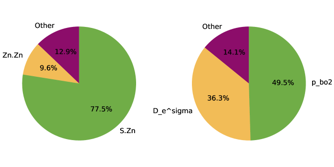
Figure 5: Grouped sensitivities as determined by the HSIC calculation using the CG kernel. Grouped by parameter group (left) and parameter name (right).

The identification of these $\sigma$-bond parameters, particularly for sulphur-zinc and zinc-zinc bonds are quite reasonable given the composition of the training set. The degree to which the sensitivity is dominated by only these parameters, however, may be surprising. Nevertheless, the results seem intuitive.

5.3 Reparameterizations with sensitive parameters only

Based on the sensitivities determined above, we ran reconfigured reparameterizations using: the most sensitive $10203343$ parameters, and the least sensitive $10203343$ parameters. The most-sensitive groupings are shown in Figure 4. We made these selections so that the set of $10$ most sensitive parameters, and the set of $43$ least sensitive parameters are complementary; together they account for the original $53$ parameters. Similarly, for other combinations. Each of the reparameterizations was conducted in the same way as the original described in Section 5.1.

In a more practical setting we do not advocate blindly activating only the most sensitive $n$ parameters; we do so here only to avoid introducing human decision-making into the results. In practice, one should use the sensitivities as a guide to better understand how the training data effects the loss function, and use some human intuition when selecting parameters.

For the sake of clarity we introduce the following nomenclature to refer to the different optimizations:

O53

reparameterizations using the original 53 active parameters;

M#

reparameterizations using the most sensitive # parameters;

L#

reparameterizations using the least sensitive # parameters.

Figure 6 shows the running best loss value seen by any of the sixteen parallel optimizers for each of the optimization configurations (Section A of the supplementary information contains the results for individual optimizers). Table 3 shows the difference between the lowest loss value and initial loss value as a fraction of the initial loss value. In other words, the percentage of the initial loss which was ‘removed’ during the optimization. Unsurprisingly, O53 produces the lowest loss because it had the most degrees-of-freedom. Any reduction in the number of active parameters can be expected to worsen achievable loss values. Indeed, all the other optimizations find worse minima than the original. However, the difference between using the most sensitive and least sensitive parameters is marked.

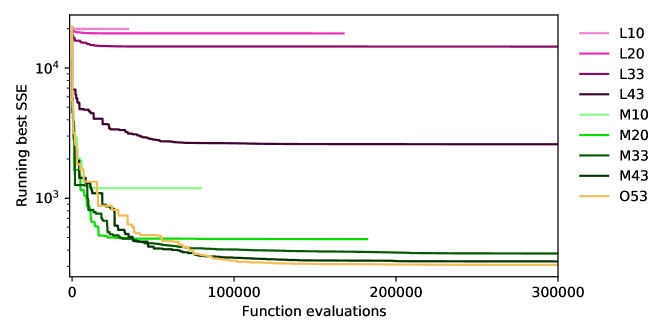
Figure 6: Running best value seen by any of the sixteen parallel optimizers for each of the optimization configurations.

Table 3: Fraction of the initial loss value which removed during optimization.

	Most Sensitive (%)	Least Sensitive (%)
10	$94.2$	$3.61$
20	$97.7$	$10.9$
33	$98.2$	$29.4$
43	$98.4$	$87.4$
53	$98.5$

In all cases using the most sensitive parameters allows us to remove $93\text{\,}\mathrm{[}$>] of the original error. In fact, some M33 and M43 optimizers find better minima than some O53 optimizers. In contrast, using the same number of least-sensitive parameters produces very poor optimizations which are unable to meaningfully reduce the loss value. Especially noteworthy is that M10 is able to locate better minima than its complement L43. Similarly, L10 is only able to reduce the loss by $4\text{\,}\mathrm{\char 37\relax}$ compared to $94\text{\,}\mathrm{\char 37\relax}$ achieved by M10.

It is also important to note that M10 and M20 are able to converge long before the $300\,000$ function evaluation limit, and use approximately one-third and two-thirds of the time used by O53. This represents significant time savings as O53 took approximately two days to complete, more than the time required to run the sensitivity analysis and M10 or M20.

These results show that our proposed HSIC sensitivity method is able to quickly identify the most sensitive parameters for reparameterization, and that a parameter selection guided by it can produce good minima in a shorter time.

5.4 Force field comparison and validation

In order to verify the quality of the new force fields, and demonstrate the risks of overfitting, we perform several validation tests using the initial force field, and the force fields with lowest error produced by O53, M10, and M20 across the sixteen optimizations each one performed.

We consider:

1. the error on the training set items;

2. an MD simulation of H2S adsorption on zincblende and wurtzite slabs;

3. an MD simulation of zincblende bulk crystal;

4. the adsorption energy of an H2S molecule on a ($110$) zincblende surface; and

5. the surface energies of ($110$) zincblende and ($11\bar{2}0$) wurtzite.

We compare the results to reference DFT calculations, as well as literature values. For calculations involving crystal surfaces, we use the ($110$) face of zincblende and ($11\bar{2}0$) face of wurtzite ZnS as they have been found to be the most energetically favorable ^{62, 52}. Slabs were always constructed from pre-optimized lattice parameters calculated with BAND using the PBEsol/DZP level of theory.

5.4.1 Training set errors

We start our analysis by decomposing the overall loss values for each of the force fields into their individual contributions. Figures 7 and 8 compare force field predictions to reference values for each of the training set items.

Figure 7 shows training set items which can be grouped together into PES scans along some coordinate. With the exception of the H2S angle scan, the original force field performs extremely poorly for these items, and in all cases the optimized force fields produce significantly improved results. The O53 force field is the most accurate for all the scans, but M20 is generally quite competitive and has similar errors. The one exception to this is the H-S bond scan in the H2S molecule which M20 did not replicate well.

Figure 8 shows the remaining training set items where we compare reference values to predictions made by the selected force fields. Although angles and forces were improved, significant errors remained in most cases and a large fraction of the original forces error remains in the final fields. Energies, which form a large part of the overall loss value, actually appear generally well-fitted and most of the error comes from a single item; this item is the energy difference between a distorted and regular ($110$) zincblende surface. We can also see that charges were effectively unimproved during the reparameterization. This is because charge related parameters were not activated in our parameter selection. Interatomic distances were the most improved class of training set items. This can be explained by the fact that the original sulphur related parameters were actually trained for oxygen, thus the initial force field bond lengths were too short to accommodate the larger sulfur atoms and had to be lengthened.

In most cases the M10 errors are substantially worse then the M20 ones. On the other hand, M20 errors are often very similar to (or in the case of angles) better than the O53 errors. In comparison to O53, M20 performs worst for forces and energies. However, as mentioned above, the bulk of the energy error is concentrated in one item, and no force field appears to predict forces very well. From these observations, there does not appear to be a strong signal that O53 is a significantly better force field than M20.

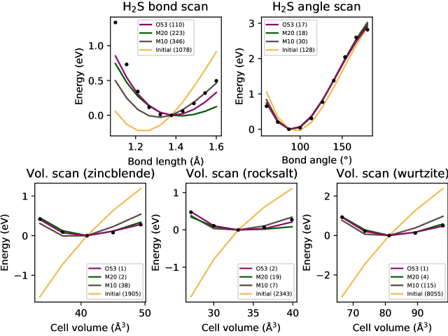
Figure 7: Training set items which form part of various PES scans. Reference values shown as black dots and loss values for each force field are shown in parentheses in the legends.

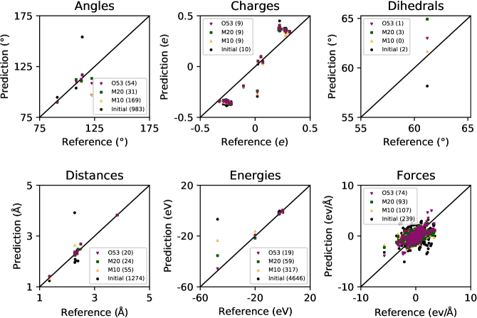
Figure 8: Comparison of reference to predicted values for each of the training set items and force fields, grouped by item type. Loss values for a group and force field are included in parentheses in the figure legends.

5.4.2 MD simulations

Adsorption to crystal surfaces

Our first validation test is an MD simulation of the adsorption of H2S molecules on ZnS slabs. We are guided by literature in constructing a realistic simulation scenario. Zhang et al. ⁶² showed computationally and experimentally that cubic ZnS with a particle size smaller than $\sim$$7\text{\,}\mathrm{nm}$ is not stable at room temperature and can easily convert to the hexagonal polymorph. Experimentally, Dloczik et al. ⁵¹ were able to produce stable ZnS columns with wall thicknesses between $10\text{\,}\mathrm{nm}30\text{\,}\mathrm{nm}$ where both cubic and wurtzite phases were detected. Qi et al. ⁵⁵ later studied the adsorption of H2S on ZnS surfaces at room temperature.

Using these sources, we create MD simulations for both morphologies using slabs $\sim$$10\text{\,}\mathrm{nm}$ thick. The temperature is maintained at $298\text{\,}\mathrm{K}$, $100$ H2S molecules are randomly positioned above and below the slabs, and the simulations are conducted for $300\,000$ time steps of $0.25\text{\,}\mathrm{fs}$ each.

Figures 9 and 10 show the final surface geometries for the wurtzite and zincblende simulations respectively. Unsurprisingly, the initial force field performs poorly as the slabs immediately collapse. The M10 and M20 simulations, however, perform better. The slabs maintain their crystalline shapes, and adsorb the H2S molecules to the slab surfaces.

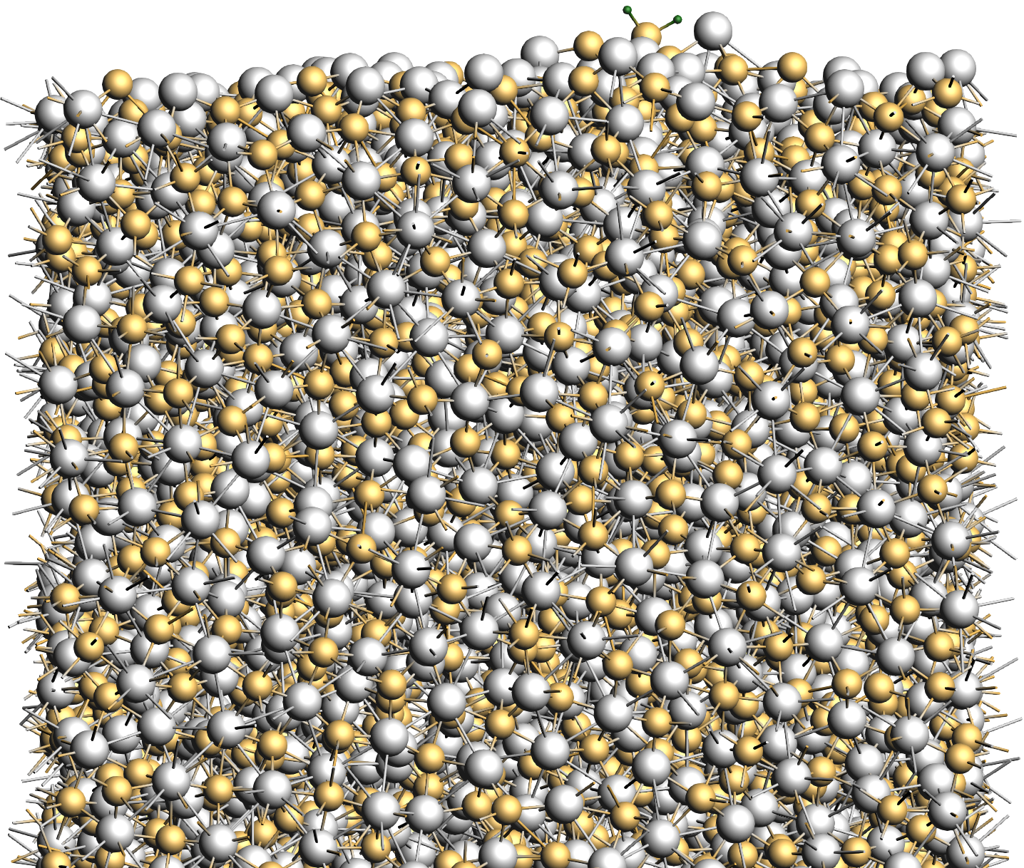
(a) Initial force field

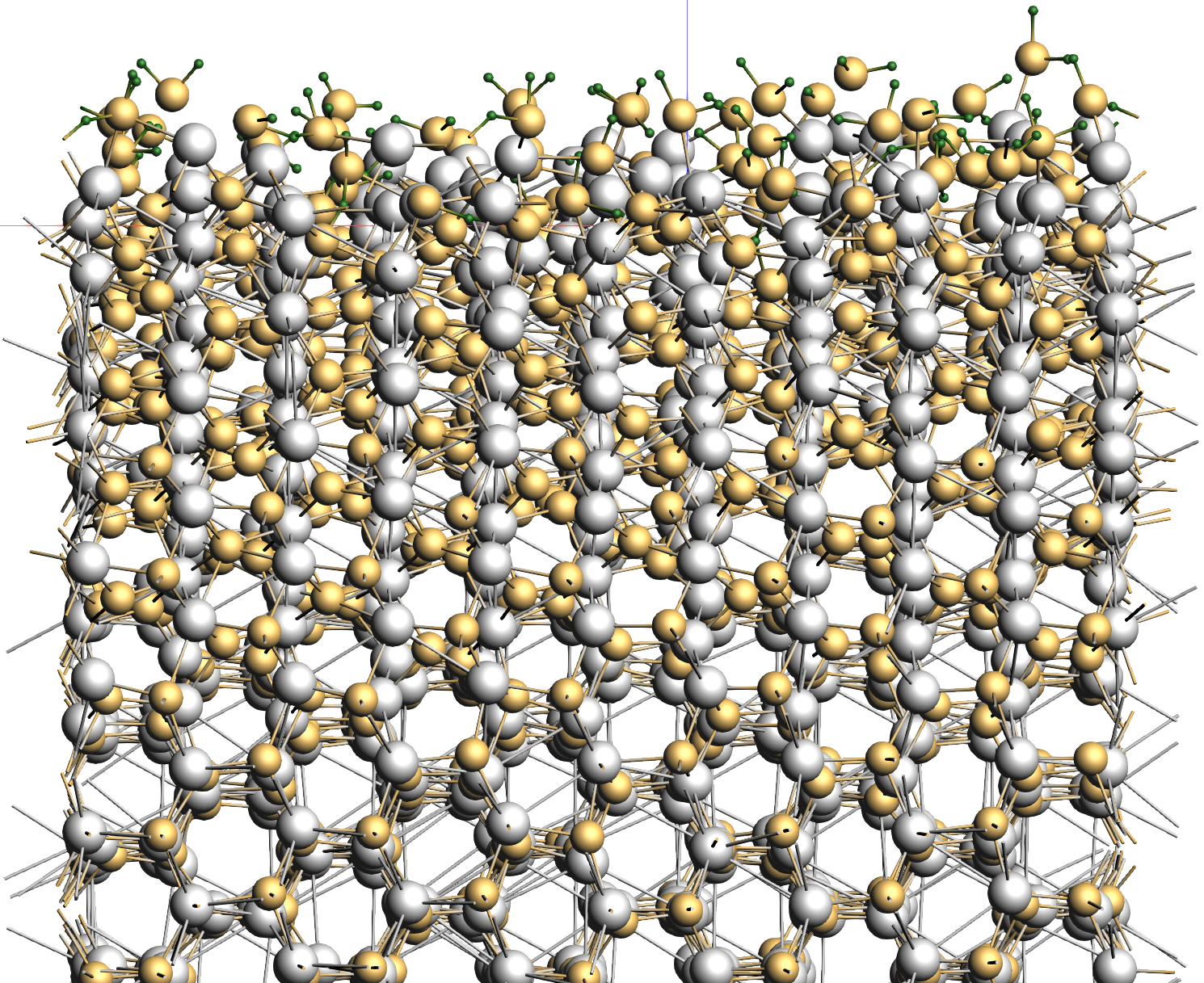
(b) O53

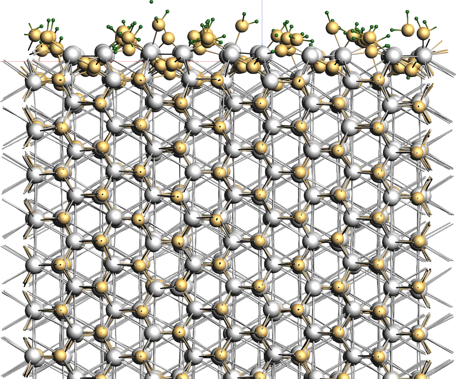
(c) M10

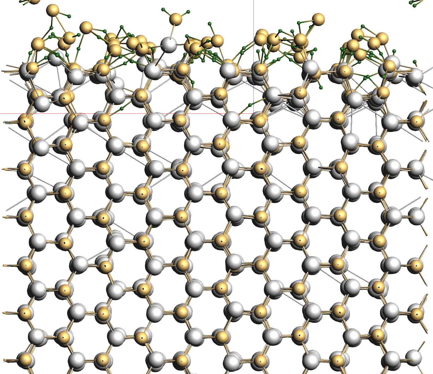
(d) M20

Figure 9: One surface in the final frames of $75\text{\,}\mathrm{ps}$ MD simulations of $100$ H2S gas molecules above and below a $10\text{\,}\mathrm{nm}$ thick wurtzite slab with ($11\bar{2}0$) surfaces using a) the initial, b) O53, c) M10, and d) M20 force fields. Sulfur atoms in yellow, zinc in silver, hydrogen in green.

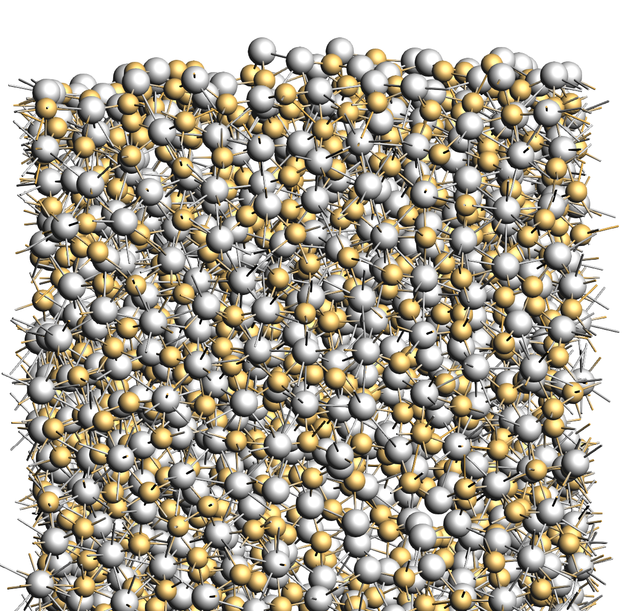
(a) Initial force field

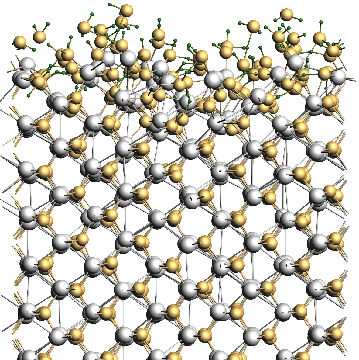
(b) O53

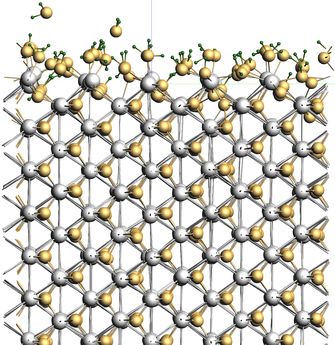
(c) M10

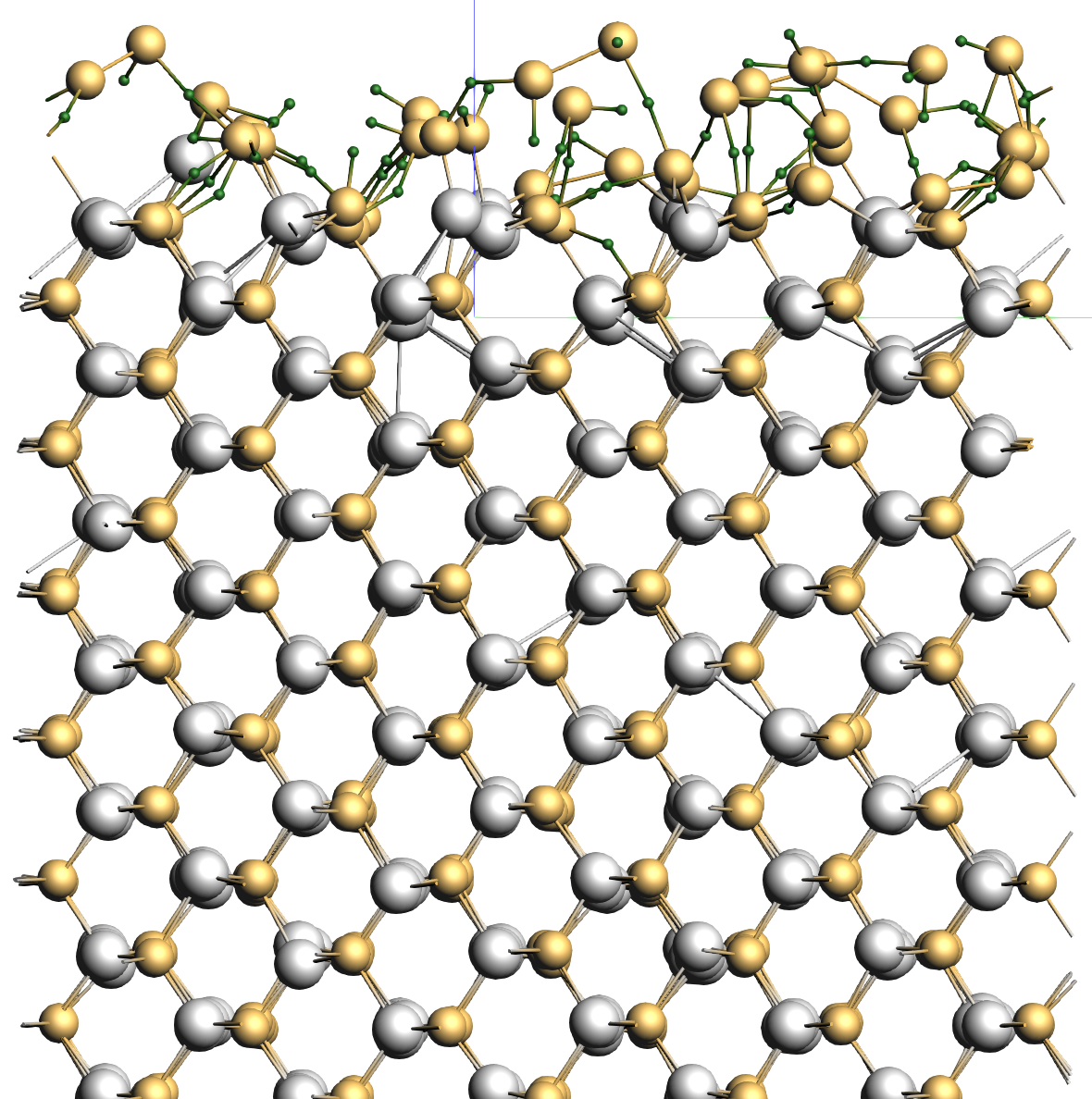
(d) M20

Figure 10: One surface in the final frames of $75\text{\,}\mathrm{ps}$ MD simulations of $100$ H2S gas molecules above and below a $10\text{\,}\mathrm{nm}$ thick zincblende slab with ($110$) surfaces using a) the initial, b) O53, c) M10, and d) M20 force fields. Sulfur atoms in yellow, zinc in silver, hydrogen in green.

The O53 simulations do not behave in the same way. These slabs struggle to maintain their surfaces. In the wurtzite case the surface layers have become almost amorphous, although the bulk crystal is relatively well-maintained, the extent of the deformation extends several layers deep. The zincblende surface is more ordered, but it is not as rigidly maintained as M10 or M20, and it appears that some H2S molecules are being chemically absorbed into the structure.

As discussed above, literature suggests that these slabs should be stable rigid solids under these conditions, making the behavior of the O53 force field surprising. We will discuss the reasons for this behavior in Section 5.4.3.

Bulk crystal

The above simulation provides a qualitative indication that the lower loss value of the O53 force field does not guarantee better performance. However, we would like to demonstrate quantitatively that M20 parameterizations produce more robust results.

To do this we ran a second MD simulation of a bulk zincblende crystal ($64$ atoms total) at $500\text{\,}\mathrm{K}$ for $10\text{\,}\mathrm{ps}$ using a time step of $0.5\text{\,}\mathrm{fs}$. Two simulations were run: one used the best force fields produced by each of the sixteen M20 optimizers, and the other used the best force fields produced by each of the sixteen O53 optimizers. In each simulation the force fields were used as a committee. In other words, each force field was applied to the same crystal geometries at each time step. The forces of these results were then averaged to update the atomic positions for the next time step.

Figure 11 shows the standard deviation of the forces across the sixteen force fields. We are not interested in the results at particular times, for particular atoms, or in particular directions, because the forces always average out to zero. Thus, the histograms simply show all the standard deviations regardless of the above distinctions. The sixteen M20 force fields show significantly more agreement than the O53 ones. This suggests that the lower dimensional optimization is much more robust, and produces force fields with a tighter distribution of results. The higher dimensional optimization has many more minima in which optimizers might be trapped. Since these extra minima are created by the presence of insensitive parameters, they are more likely to represent overfittings than genuine attractors driven by important parameters. Interestingly, the favorable spread of results seen here for M20, could not be assumed from the spread in loss values amongst its sixteen force fields which was $98$ compared to $33$ for O53.

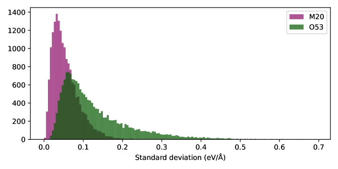
Figure 11: Standard deviation on the forces felt by all atoms, in all directions, at all time steps in bulk simulations of zincblende crystal using committee simulations of the sixteen M20 and O53 force fields.

5.4.3 Adsorption and surface energies

Our more quantitative validation tests are:

1. the calculation of the adsorption energy ($E_{\mathrm{ads}}$) of an H2S molecule on the ($110$) surface of zincblende; and

2. surface energy ($E_{\mathrm{surf}}$) calculations for the ($110$) surface of zincblende and ($11\bar{2}0$) surface of wurtzite.

Details of these calculations are included in Section C and Section D of the supplementary information, respectively.

In this case we use the best force fields from every optimizer in the O53 and M20 sets to analyse the distribution of results. We do not consider all sixteen M10 results as they perform poorly. The results are shown in Figure 12 as a function of the force fields’ associated SSE. Detailed results for individual optimizers can be found in Section E of the supplementary information. In these plots, we have also included DFT, initial force field, and best M10 force field results for comparison. The initial and M10 results are not shown with their corresponding loss values as they are too large and would make the plots illegible. In the discussions that follow, we will continue to use ‘best’ to refer to the force field with the lowest loss value (SSE), it does not mean the force field with the most accurate validation result.

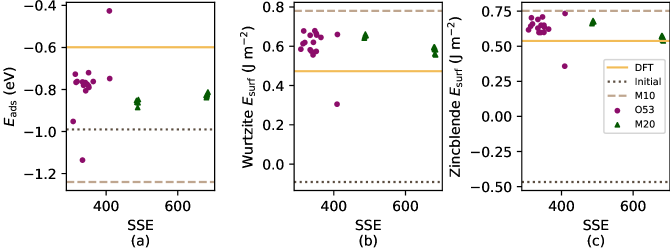
Figure 12: a) H2S adsorption energy, b) wurtzite ($11\bar{2}0$) surface energy, and c) zincblende ($110$) surface energy versus SSE for the best force fields found by each of the sixteen optimizers run in the O53 and M20 reparameterizations. Reference DFT results shown with horizontal yellow line.

Adsorption energy

We begin our comments by considering the adsorption energy results. None of the force fields are very accurate in this regard in comparison to our DFT reference, however the best M20 force field is more accurate than that from O53. Interestingly, the initial force field produces a better prediction than M10 and is only slightly worse than the best O53 force field. More broadly, however, all the M20 force fields predict adsorption energies in a narrow range from $-0.89\text{\,}\mathrm{e}\mathrm{V}-0.81\text{\,}\mathrm{e}\mathrm{V}$, which is much more reproducible than the O53 results which range from $-1.14\text{\,}\mathrm{e}\mathrm{V}-0.43\text{\,}\mathrm{e}\mathrm{V}$.

This variability might be explained by the odd behavior seen in several O53 geometry optimizations. Figure 13 shows the final frames the adsorbed molecule geometry optimizations using DFT and the best O53 force field. The H2S molecule is initially placed close to the zinc atom highlighted in blue, and settles into this position using DFT. However, using the O53 force field, the H2S molecule moves away from this atom towards a row of sulfur atoms which are, in turn, repelled by it. The geometry optimization is converged, which means that this desorbed position with deformed surface is more energetically favorable than an adsorbed position on zinc—which is incorrect. It is possible that the strange surface effects seen in Section 5.4.2 may be associated with this.

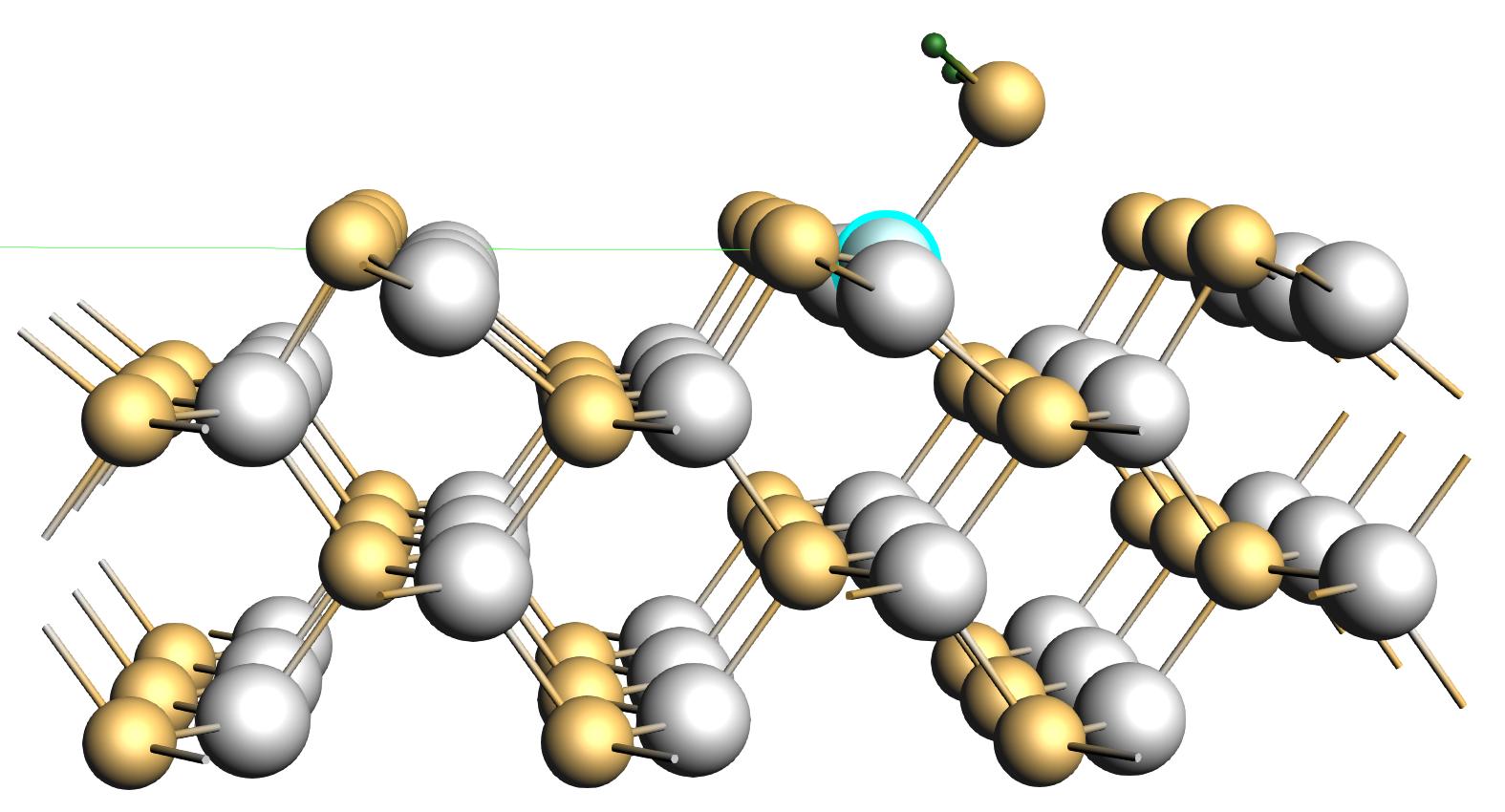
(a)

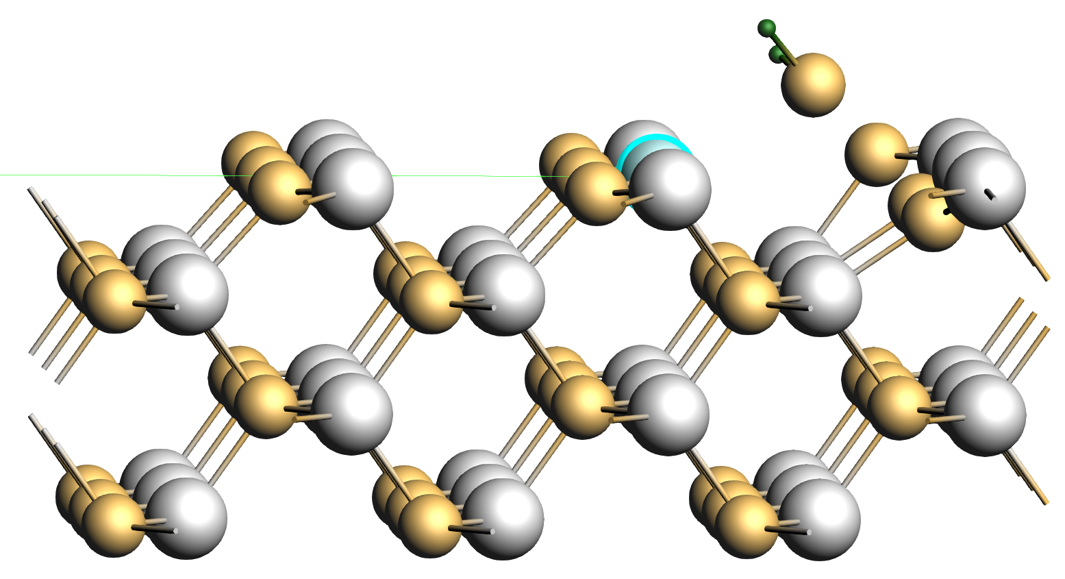
(b)

Figure 13: Final frame of a geometry optimization of an H2S molecule adsorbed on a ($110$) zincblende surface using a) DFT and b) the best O53 force field. The molecule is originally positioned near the zinc atom in blue.

Surface energy

If we consider the surface energy results, the distributions of the O53 force fields are consistently larger than those of the M20 results. On average, the O53 results are similarly accurate to M20 for the wurtzite surface. For the zincblende surface, one of the M20 clusters is actually quite accurate.

Overall, none of the force fields performed generally well across all the validation tests, but they are improvements to the initial force field. If more accuracy is desired, then more attention needs to be given to the composition of the training set, however, this is not the focus of this article.

Correlations with loss values

The most interesting conclusions from these results, come from comparing them to the force fields’ associated SSE. All sixteen O53 optimizers found SSE values tightly clustered between $308$ and $410$, much lower and less variable than the M20 optimizers that are clustered around two values between $485$ and $684$. If one only considers the loss values, then one might expect that predictions made by the O53 force fields will be similarly more precise than those of M20, however, we see that this is not the case. O53 validation results are significantly more variable than those of M20 and, on average, seem to be only slightly more accurate.

Most crucially, the high variability of the O53 validations are not correlated with the SSE. In other words, a better prediction of the training set items is not correlated with a more accurate prediction of the validation tests. We believe that these facts, and the unusual behavior of the O53 MD simulations in Section 5.4.2, can be attributed to overfitting. Interestingly, the M20 results seem to be inversely correlated with the loss values, i.e., a higher loss leads to a more accurate validation result. This might suggest that M20 is also seeing some overfitting effects, however, there is not enough data to verify this because all optimizers fall near one of only two SSE values.

Overfitting is a common occurrence during ReaxFF reparameterization ^{50, 13, 9} and becomes more likely as more parameters are allowed to change. These validation tests highlight the dangers of activating too many dimensions during a reparameterization as more degrees of freedom create opportunities for overfitting. We present two dangers which occur when too many parameters are used.

First, it is important to emphasize the difference between a parameter’s sensitivity to some loss function (which is a function of a user-generated training set), and its true importance in the potential function. If a training set does not include enough items to capture the importance of a parameter, then it will register as insensitive. If an important, but insensitive, parameter is activated during reparameterization then the optimizer will change it quasi-randomly. This can result in force fields with very low loss values, that perform very poorly in production runs; sensitive parameters have been set correctly, but other important ones have been changed incorrectly.

A second danger is the fact that parameters can have a compensatory effect. If many parameters are active, then it is possible that multiple parameter sets can satisfy the training data, but the potential will perform poorly during simulation. By using too many parameters the optimizers have an opportunity to move insensitive ones to reduce the loss rather than identifying the ‘correct’ values for a small number of appropriate parameters.

In our example, the $53$ dimension reparameterizations seem to have activated too many dimensions. Although they produced the lowest overall loss values, they did not achieve the lowest loss for every class of items, nor did they always make the most accurate or precise predictions in our validation tests. In the MD simulations we see odd behavior which, along with the precision problems discussed previously, we believe to be evidence of overfitting.

Conversely, the reparameterizations using only the $10$ most sensitive parameters seem to not have had enough degrees of freedom. These force fields produce significant training set errors compared to O53 and M20, and perform poorly in the validation tests.

Using $20$ of the most sensitive parameters produces good quality force fields which perform better than the O53 force fields in some tests, despite having marginally worse training set losses. The results of the validation tests were also consistently more precise than those of O53, and of comparable accuracy. The MD simulation aligned with expectations, and the force fields were produced in a shorter time than that required for the original optimization.

6 Outlook

We believe that there are several areas available which warrant further study. First, the training set used here could be used as a starting point to produce a better quality force field for Zn/S/H. This would require a significant expansion of the training set, and involve all of the well-known and thorny issues associated with training set design ⁵⁰.

Second, a parameter’s sensitivity is a strong function of the range in which it is allowed to vary. In this work, we have not needed to give this much consideration since the ParAMS package provides recommended ranges. However, it is not certain that these are always appropriate. A formalisation of appropriate ranges, or a robust mechanism to determine them would go a long way to ensuring that sensitivities are being appropriately determined.

Third, we have identified sampling as the limiting step of the sensitivity procedure. It may be interesting to investigate the extraction of samples from optimizer trajectories. However, since the HSIC requires uniformly distributed random samples, one would need to extract samples carefully from the trajectories. One possibility is the Kennard-Stone algorithm ⁶³, but this is slow and sequential. Nevertheless, ‘closing the loop’ and allowing users to extract sensitivities from optimization results seems like an appealing prospect.

7 Conclusions

As an introductory work, we have demonstrated that an HSIC sensitivity analysis applied to a ReaxFF reparameterization can successfully identify the most sensitive parameters. We have further shown that using only the most sensitive parameters during optimization leads to faster convergence and a reduced chance of overfitting. Even qualitatively, the use of such a sensitivity analysis can provide valuable insights for the user into the composition of the training set. Overall, we believe that the HSIC sensitivity analysis is a useful, robust, and easy to use tool which has the potential to greatly aid in the reparameterization of ReaxFF force fields.

Author Contributions

MG designed and implemented the sensitivity test, ran the test work, and wrote this article. MH designed the training set and guided some of the validation tests. TV provided supervision, revisions, guidance, and advice.

The authors thank the Flemish Supercomputing Centre (VSC), funded by Ghent University, FWO and the Flemish Government for use of their computational resources.

Funding for the project was provided by the European Union’s Horizon 2020 research and innovation program under grant agreement No. 814143. TV and MG are also supported by the Research Board of Ghent University (BOF) under award No. 01IT2322.

The following items are included in the Supplementary Information:

si.pdf

full optimization results, calculation methodologies for adsorption and surface energies, full adsorption and surface energy results, training set composition;

job_collection.yaml

training set geometries and job calculation settings;

engine_collection.yaml

task settings for the input geometries;

training_set.yaml

reference values, weights, and sigma values for training data;

initial_parameters.yaml

original ReaxFF parameter values and ranges (O53 parameters set as active).

The YAML files are human-readable and used by ParAMS ¹⁴.

This information is available free of charge via the Internet at http://pubs.acs.org.

References

- van Duin et al. 2001 van Duin, A. C. T.; Dasgupta, S.; Lorant, F.; Goddard, W. A. ReaxFF: a reactive force field for hydrocarbons. The Journal of Physical Chemistry A 2001, 105, 9396–9409
- Senftle et al. 2016 Senftle, T. P.; Hong, S.; Islam, M. M.; Kylasa, S. B.; Zheng, Y.; Shin, Y. K.; Junkermeier, C.; Engel-Herbert, R.; Janik, M. J.; Aktulga, H. M.; Verstraelen, T.; Grama, A.; van Duin, A. C. T. The ReaxFF reactive force-field: development, applications and future directions. npj Computational Materials 2016, 2, 15011
- Komissarov et al. 2021 Komissarov, L.; Rüger, R.; Hellström, M.; Verstraelen, T. ParAMS: parameter optimization for atomistic and molecular simulations. Journal of Chemical Information and Modeling 2021, 61, 3737–3743
- Freitas Gustavo and Verstraelen 2022 Freitas Gustavo, M.; Verstraelen, T. GloMPO (globally managed parallel optimization): a tool for expensive, black-box optimizations, application to ReaxFF reparameterizations. Journal of Cheminformatics 2022, 14, 7
- Chenoweth et al. 2008 Chenoweth, K.; van Duin, A. C.; Goddard, W. A. ReaxFF reactive force field for molecular dynamics simulations of hydrocarbon oxidation. Journal of Physical Chemistry A 2008, 112, 1040–1053
- Barcaro et al. 2017 Barcaro, G.; Monti, S.; Sementa, L.; Carravetta, V. Parametrization of a reactive force field (ReaxFF) for molecular dynamics simulations of Si nanoparticles. Journal of Chemical Theory and Computation 2017, 13, 3854–3861
- Bae and Aikens 2013 Bae, G.-T.; Aikens, C. M. Improved ReaxFF force field parameters for Au–S–C–H systems. Journal of Physical Chemistry A 2013, 117, 10438–10446
- Liu et al. 2020 Liu, Y.; Hu, J.; Hou, H.; Wang, B. Development and application of a ReaxFF reactive force field for molecular dynamics of perfluorinatedketones thermal decomposition. Chemical Physics 2020, 538, 110888
- Hubin et al. 2016 Hubin, P. O.; Jacquemin, D.; Leherte, L.; Vercauteren, D. P. Parameterization of the ReaxFF reactive force field for a proline-catalyzed aldol reaction. Journal of Computational Chemistry 2016, 37, 2564–2572
- Hu et al. 2017 Hu, X.; Schuster, J.; Schulz, S. E. Multiparameter and parallel optimization of ReaxFF reactive force field for modeling the atomic layer deposition of copper. Journal of Physical Chemistry C 2017, 121, 28077–28089
- LaBrosse et al. 2010 LaBrosse, M. R.; Johnson, J. K.; van Duin, A. C. Development of a transferable reactive force field for cobalt. Journal of Physical Chemistry A 2010, 114, 5855–5861
- Larsson et al. 2013 Larsson, H. R.; van Duin, A. C.; Hartke, B. Global optimization of parameters in the reactive force field ReaxFF for SiOH. Journal of Computational Chemistry 2013, 34, 2178–2189
- Shchygol et al. 2019 Shchygol, G.; Yakovlev, A.; Trnka, T.; van Duin, A. C.; Verstraelen, T. ReaxFF parameter optimization with Monte–Carlo and evolutionary algorithms: guidelines and insights. Journal of Chemical Theory and Computation 2019, 15, 6799–6812
- Software for Chemistry and Materials 2022 Software for Chemistry and Materials, Parameterization tools for AMS (2022.204.r105828). 2022; https://www.scm.com/doc/params [Accessed: June 2022]
- Saltelli et al. 2019 Saltelli, A.; Aleksankina, K.; Becker, W.; Fennell, P.; Ferretti, F.; Holst, N.; Li, S.; Wu, Q. Why so many published sensitivity analyses are false: a systematic review of sensitivity analysis practices. Environmental Modelling & Software 2019, 114, 29–39
- Baroni and Francke 2020 Baroni, G.; Francke, T. An effective strategy for combining variance- and distribution-based global sensitivity analysis. Environmental Modelling & Software 2020, 134, 104851
- Spagnol et al. 2019 Spagnol, A.; Le Riche, R.; Da Veiga, S. Global sensitivity analysis for optimization with variable selection. SIAM/ASA Journal on Uncertainty Quantification 2019, 7, 417–443
- Borgonovo 2007 Borgonovo, E. A new uncertainty importance measure. Reliability Engineering & System Safety 2007, 92, 771–784
- Saltelli et al. 2008 Saltelli, A.; Ratto, M.; Andres, T.; Campolongo, F.; Cariboni, J.; Gatelli, D.; Saisana, M.; Tarantola, S. Global Sensitivity Analysis. The Primer; John Wiley & Sons, Ltd, 2008
- Herman et al. 2013 Herman, J. D.; Kollat, J. B.; Reed, P. M.; Wagener, T. Technical note: method of Morris effectively reduces the computational demands of global sensitivity analysis for distributed watershed models. Hydrology and Earth System Sciences 2013, 17, 2893–2903
- Nossent et al. 2011 Nossent, J.; Elsen, P.; Bauwens, W. Sobol’ sensitivity analysis of a complex environmental model. Environmental Modelling & Software 2011, 26, 1515–1525
- Campolongo et al. 2011 Campolongo, F.; Saltelli, A.; Cariboni, J. From screening to quantitative sensitivity analysis. A unified approach. Computer Physics Communications 2011, 182, 978–988
- De Lozzo and Marrel 2016 De Lozzo, M.; Marrel, A. New improvements in the use of dependence measures for sensitivity analysis and screening. Journal of Statistical Computation and Simulation 2016, 86, 3038–3058
- Da Veiga 2015 Da Veiga, S. Global sensitivity analysis with dependence measures. Journal of Statistical Computation and Simulation 2015, 85, 1283–1305
- Gretton et al. 2005 Gretton, A.; Bousquet, O.; Smola, A.; Schölkopf, B. In Algorithmic Learning Theory; Jain, S., Simon, H. U., Tomita, E., Eds.; Springer Berlin Heidelberg, 2005; pp 63–77
- Yamada et al. 2018 Yamada, M.; Tang, J.; Lugo-Martinez, J.; Hodzic, E.; Shrestha, R.; Saha, A.; Ouyang, H.; Yin, D.; Mamitsuka, H.; Sahinalp, C.; Radivojac, P.; Menczer, F.; Chang, Y. Ultra high-dimensional nonlinear feature selection for big biological data. IEEE Transactions on Knowledge and Data Engineering 2018, 30, 1352–1365
- Yamada et al. 2014 Yamada, M.; Jitkrittum, W.; Sigal, L.; Xing, E. P.; Sugiyama, M. High-dimensional feature selection by feature-wise kernelized lasso. Neural Computation 2014, 26, 185–207
- Song et al. 2012 Song, L.; Smola, A.; Gretton, A.; Bedo, J.; Borgwardt, K. Feature selection via dependence maximization. Journal of Machine Learning Research 2012, 13, 1393–1434
- Climente-González et al. 2019 Climente-González, H.; Azencott, C.-A.; Kaski, S.; Yamada, M. Block HSIC lasso: model-free biomarker detection for ultra-high dimensional data. Bioinformatics 2019, 35, i427–i435
- Feng et al. 2018 Feng, L.; Di, T.; Zhang, Y. HSIC-based kernel independent component analysis for fault monitoring. Chemometrics and Intelligent Laboratory Systems 2018, 178, 47–55
- Qian et al. 2022 Qian, J.; Lu, M.; Tian, F.; Liu, R. Study on sensor array optimization of medical electronic nose for wound infection detection. IEEE Transactions on Circuits and Systems II: Express Briefs 2022, 69, 1867–1871
- Li et al. 2021 Li, Y.; Pogodin, R.; Sutherland, D. J.; Gretton, A. In Advances in Neural Information Processing Systems; Ranzato, M., Beygelzimer, A., Dauphin, Y., Liang, P. S., Vaughan, J. W., Eds.; Curran Associates, Inc., 2021; Vol. 34; pp 15543–15556
- Wang and Li 2018 Wang, T.; Li, W. Kernel learning and optimization with Hilbert–Schmidt independence criterion. International Journal of Machine Learning and Cybernetics 2018, 9, 1707–1717
- Kaymak et al. 2022 Kaymak, M. C.; Rahnamoun, A.; O’Hearn, K. A.; van Duin, A. C. T.; Merz, K. M. J.; Aktulga, H. M. JAX–ReaxFF: a gradient-based framework for fast optimization of reactive force fields. Journal of Chemical Theory and Computation 2022, 18, 5181–5194
- Pahari and Chaturvedi 2012 Pahari, P.; Chaturvedi, S. Determination of best-fit potential parameters for a reactive force field using a genetic algorithm. Journal of Molecular Modeling 2012, 18, 1049–1061
- Trnka et al. 2018 Trnka, T.; Tvaroška, I.; Koča, J. Automated training of ReaxFF reactive force fields for energetics of enzymatic reactions. Journal of Chemical Theory and Computation 2018, 14, 291–302
- Jaramillo-Botero et al. 2014 Jaramillo-Botero, A.; Naserifar, S.; Goddard, W. A. General multiobjective force field optimization framework, with application to reactive force fields for silicon carbide. Journal of Chemical Theory and Computation 2014, 10, 1426–1439
- Boothroyd et al. 2022 Boothroyd, S.; Wang, L.-P.; Mobley, D. L.; Chodera, J. D.; Shirts, M. R. Open force field evaluator: an automated, efficient, and scalable framework for the estimation of physical properties from molecular simulation. Journal of Chemical Theory and Computation 2022, 18, 3566–3576
- Örn Jónsson et al. 2022 Örn Jónsson, E.; Rasti, S.; Galynska, M.; Meyer, J.; Jónsson, H. Transferable potential function for flexible H2O molecules based on the single-center multipole expansion. Journal of Chemical Theory and Computation 2022, 18, 7528–7543
- Mondal et al. 2020 Mondal, A.; Young, J. M.; Barckholtz, T. A.; Kiss, G.; Koziol, L.; Panagiotopoulos, A. Z. Genetic algorithm driven force field parameterization for molten alkali-metal carbonate and hydroxide salts. Journal of Chemical Theory and Computation 2020, 16, 5736–5746
- Verstraelen et al. 2011 Verstraelen, T.; Bultinck, P.; van Speybroeck, V.; Ayers, P. W.; van Neck, D.; Waroquier, M. The significance of parameters in charge equilibration models. Journal of Chemical Theory and Computation 2011, 7, 1750–1764
- He et al. 2022 He, Z.; Xiong, X.; Yang, B.; Li, H. Aerodynamic optimisation of a high-speed train head shape using an advanced hybrid surrogate-based nonlinear model representation method. Optimization and Engineering 2022, 23, 59–84
- Wang et al. 2022 Wang, T.; Wang, C.; Xu, Z.; Cui, C.; Wang, X.; Demitrack, Z.; Dai, Z.; Bagtzoglou, A.; Stuber, M. D.; Li, B. Precise control of water and wastewater treatment systems with non-ideal heterogeneous mixing models and high-fidelity sensing. Chemical Engineering Journal 2022, 430, 132819
- Zhang et al. 2020 Zhang, T.; Di, X.; Chen, G.; Zhu, L. Parameterization of a COMPASS force field for single layer blue phosphorene. Nanotechnology 2020, 31, 145702
- Gopalakrishnan et al. 2020 Gopalakrishnan, S.; Dash, S.; Maranas, C. K-FIT: an accelerated kinetic parameterization algorithm using steady-state fluxomic data. Metabolic Engineering 2020, 61, 197–205
- Mohammed and Gnedin 2018 Mohammed, I.; Gnedin, N. Y. Baryonic effects in cosmic shear tomography: PCA parameterization and the importance of extreme baryonic models. The Astrophysical Journal 2018, 863, 173
- Quinn et al. 2019 Quinn, K. N.; Wilber, H.; Townsend, A.; Sethna, J. P. Chebyshev approximation and the global geometry of model predictions. Physical Review Letters 2019, 122, 158302
- Mortier et al. 1986 Mortier, W. J.; Ghosh, S. K.; Shankar, S. Electronegativity-equalization method for the calculation of atomic charges in molecules. Journal of the American Chemical Society 1986, 108, 4315–4320
- Verstraelen et al. 2013 Verstraelen, T.; Ayers, P. W.; van Speybroeck, V.; Waroquier, M. ACKS2: atom-condensed Kohn–Sham DFT approximated to second order. The Journal of Chemical Physics 2013, 138, 074108
- Müller and Hartke 2016 Müller, J.; Hartke, B. ReaxFF reactive force field for disulfide mechanochemistry, fitted to multireference ab initio data. Journal of Chemical Theory and Computation 2016, 12, 3913–3925
- Dloczik et al. 2001 Dloczik, L.; Engelhardt, R.; Ernst, K.; Fiechter, S.; Sieber, I.; Könenkamp, R. Hexagonal nanotubes of ZnS by chemical conversion of monocrystalline ZnO columns. Applied Physics Letters 2001, 78, 3687
- Hamad et al. 2002 Hamad, S.; Cristol, S.; Catlow, C. R. A. Surface structures and crystal morphology of ZnS: computational study. Journal of Physical Chemistry B 2002, 106, 11002–11008
- Li et al. 2021 Li, S.; Wei, X.; Zhu, S.; Gui, Y. First principles analysis of SO2, H2S adsorbed on Fe–ZnS surface. Sensors and Actuators A: Physical 2021, 329, 112827
- Raymand et al. 2010 Raymand, D.; van Duin, A. C.; Spangberg, D.; Goddard, W. A.; Hermansson, K. Water adsorption on stepped ZnO surfaces from MD simulation. Surface Science 2010, 604, 741–752
- Qi et al. 2014 Qi, G.; Zhang, L.; Yuan, Z. Improved H2S gas sensing properties of ZnO nanorods decorated by a several nm ZnS thin layer. Physical Chemistry Chemical Physics 2014, 16, 13434–13439
- Software for Chemistry and Materials 2022 Software for Chemistry and Materials, Force field format specification. 2022; https://tinyurl.com/5aerwd38 [Accessed: June 2022]
- Islam et al. 2015 Islam, M. M.; Ostadhossein, A.; Borodin, O.; Yeates, A. T.; Tipton, W. W.; Hennig, R. G.; Kumar, N.; van Duin, A. C. T. ReaxFF molecular dynamics simulations on lithiated sulfur cathode materials. Physical Chemistry Chemical Physics 2015, 17, 3383–3393
- Software for Chemistry and Materials 2022 Software for Chemistry and Materials, ReaxFF: SCM developer documentation. 2022; https://tinyurl.com/39vkburf [Accessed: June 2022]
- Verstraelen et al. 2016 Verstraelen, T.; Vandenbrande, S.; Heidar-Zadeh, F.; Vanduyfhuys, L.; van Speybroeck, V.; Waroquier, M.; Ayers, P. W. Minimal basis iterative stockholder: atoms in molecules for force-field development. Journal of Chemical Theory and Computation 2016, 12, 3894–3912
- Hansen and Ostermeier 2001 Hansen, N.; Ostermeier, A. Completely derandomized self-adaptation in evolution strategies. Evolutionary computation 2001, 9, 159–195
- Gretton et al. 2012 Gretton, A.; Borgwardt, K. M.; Rasch, M. J.; Schölkopf, B.; Smola, A. A kernel two-sample test. Journal of Machine Learning Research 2012, 13, 723–773
- Zhang et al. 2003 Zhang, H.; Huang, F.; Gilbert, B.; Banfield, J. F. Molecular dynamics simulations, thermodynamic analysis, and experimental study of phase stability of zinc sulfide nanoparticles. Journal of Physical Chemistry B 2003, 107, 13051–13060
- Kennard and Stone 1969 Kennard, R. W.; Stone, L. A. Computer aided design of experiments. Technometrics 1969, 11, 137–148