Re-imagine the Negative Prompt Algorithm:
Transform 2D Diffusion into 3D, alleviate Janus problem and Beyond
Abstract
Although text-to-image diffusion models have made significant strides in generating images from text, they are sometimes more inclined to generate images like the data on which the model was trained rather than the provided text. This limitation has hindered their usage in both 2D and 3D applications. To address this problem, we explored the use of negative prompts but found that the current implementation fails to produce desired results, particularly when there is an overlap between the main and negative prompts. To overcome this issue, we propose Perp-Neg, a new algorithm that leverages the geometrical properties of the score space to address the shortcomings of the current negative prompts algorithm. Perp-Neg does not require any training or fine-tuning of the model. Moreover, we experimentally demonstrate that Perp-Neg provides greater flexibility in generating images by enabling users to edit out unwanted concepts from the initially generated images in 2D cases. Furthermore, to extend the application of Perp-Neg to 3D, we conducted a thorough exploration of how Perp-Neg can be used in 2D to condition the diffusion model to generate desired views, rather than being biased toward the canonical views. Finally, we applied our 2D intuition to integrate Perp-Neg with the state-of-the-art text-to-3D (DreamFusion) method, effectively addressing its Janus (multi-head) problem.
1 Introduction
Advancements in generating images using diffusion models from text have shown remarkable capabilities in producing a wide range of creative images from unstructured text inputs [2, 35, 37, 38, 48]. However, research has found that the generated images may not always accurately represent the intended meaning of the original text prompt [3, 5, 13, 46].
Generating satisfactory images that semantically match the text query is challenging, as it requires textual concepts to match the images at a grounded level. However, due to the difficulty of obtaining such a fine-grained annotation, current text-to-image models have difficulty fully understanding the relationship between text and images. Therefore, they are inclined to generate images like high-frequent text-image pairs in the datasets, where we can observe that the generated images are missing requested or containing undesired attributes [19]. Most of the recent works focus on adding back the missing objects or attributes to existing content to edit images based on a well-designed main text prompt [1, 3, 5, 6, 11, 17, 23, 24, 41]. However, limited of them study how to remove redundant attributes, or force the model NOT to have an unwanted object using negative prompts [10], which is the main goal of our paper.
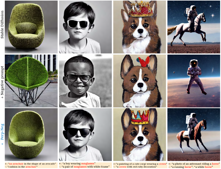
We start this paper by showing the shortcoming of the current negative prompt algorithm. After our initial investigation, we realized the current implementation of using negative prompts could produce unsatisfactory results when there is an overlap between the main prompt and the negative ones, as shown in the examples in Figure 2. To address the above problem, we propose Perp-Neg algorithm, which does not require any training and can readily be applied to a pre-trained diffusion model. We refer to our method as Perp-Neg since it employs the perpendicular score estimated by the denoiser for the negative prompt. More specifically, Perp-Neg limits the direction of denoising, guided by the negative prompt to be always perpendicular to the direction of the main prompt. In this way, the model is able to eliminate the undesired perspectives in the negative prompts without changing the main semantics, as illustrated in Figure 2.
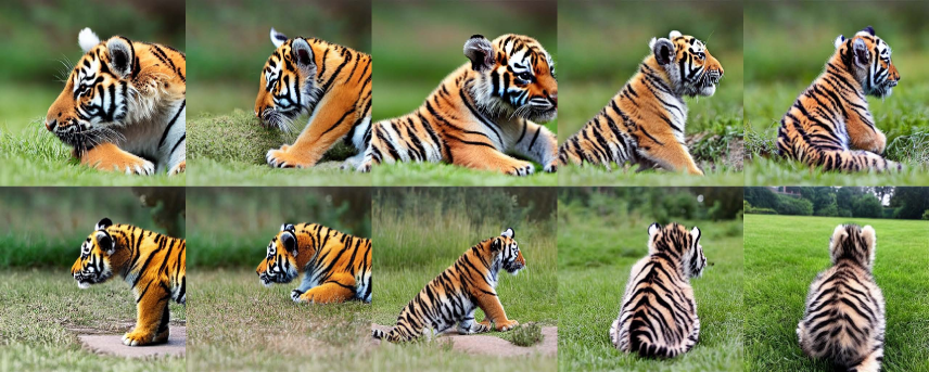
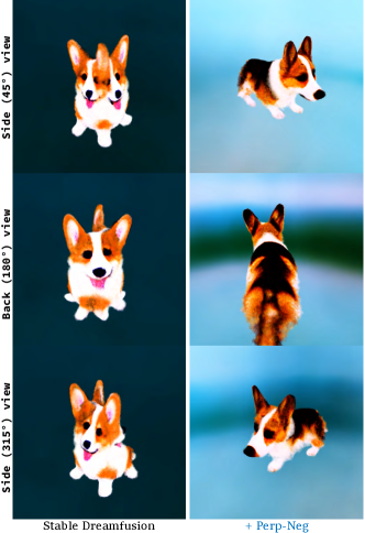
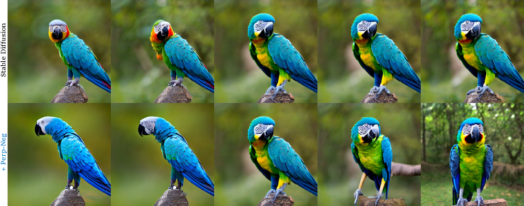
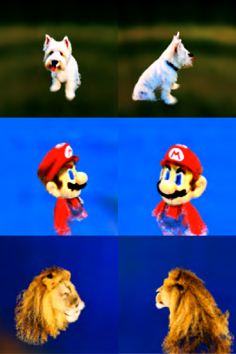
Furthermore, We extend Perp-Neg to DreamFusion[31], a state-of-the-art text-to-3D model, and show how Perp-Neg can alleviate its Janus problem, which refers to the case that a 3D-generated object inaccurately shows the canonical view of the object from several viewpoints, as shown in the left column of Figure 1. Recent studies have considered that the main cause of the Janus problem is the failure of the pre-trained 2D diffusion model in following the view instruction provided in the prompt [25]. Therefore, we first, in 2D, show quantitatively and qualitatively how our algorithm can significantly improve the view fidelity of a pretrained diffusion model. We also explore how Perp-Neg can be employed for effective interpolation between two views of an object in 2D as it is needed for 3D cases, as illustrated in Figure 3. Then we integrate Perp-Neg in Stable DreamFusion and show how it can alleviate the Janus problem.
Our contributions can be summarized as follows:
-
•
We find the limitations of the current negative prompt implementation which is susceptible to the overlap between a positive and a negative prompt.
-
•
We propose Perp-Neg, a sampling algorithm for text-to-image diffusion models to eliminate undesired attributes indicated by the negative prompt while preserving the main concept, without any training needed.
-
•
Our experiments quantitatively and qualitatively demonstrate that Perp-Neg significantly improves diffusion model prompt fidelity in view generation.
-
•
By enhancing the 2D diffusion model in following the view instruction, we mitigate the Janus problem in text-to-3D generation tasks.
2 Perp-Neg: Novel negative prompt algorithm
2.1 Preliminary
Diffusion Models: Diffusion-based (also known as score-matching) models [14, 39, 40] is a family of generative models that employ a forward process and a reverse process to iteratively corrupt and generate the data within steps. Specifically, denoting as the data distribution and as the generative prior, such two processes can be modeled as the following:
| (1) |
One of the most appealing attributes of diffusion models is that any intermediate step of the forward process and every single step in the reverse process can be modeled as a Gaussian distribution like formulated in [14]:
| (2) |
where and can be explicitly calculated with a pre-defined variance schedule . Moreover, the generator is a linear combination of and a trainable generator that predicts the noise in , which is usually optimized with a simple weighted noise prediction loss
| (3) | |||
with as the weight that depends on the timestep that is uniformly drawn from .
Text-to-Image Diffusion Models and Composing Diffusion Model: Recent works have shown the success of leveraging the power of diffusion models, where large-scale models are able to be trained on extremely large text-image paired datasets by modeling with the loss function in Equation 3 (or its variants) [28, 35, 37, 38], with the text prompt often encoded with a pre-trained large language model [8, 33]. To generate photo-realistic images given text prompts, the diffusion models can further take advantage of classifier guidance [9] or classifier-free guidance [15] to improve the image quality. Especially, in the context of text-to-image generation, classifier-free guidance is more widely used, which is usually expressed as a linear interpolation between the conditional and unconditional prediction at each timestep with a guidance scale parameter .
When the prompt becomes complex, the model may fail to understand some key elements in the query prompt and create undesired images. To handle complex textual information, [21] proposes composing diffusion models to factorize the text prompts into a set of text prompts, i.e., , and model the conditional distribution as
| (4) |
By applying Bayes rule, we have and
| (5) |
Note that and respectively correspond to and modeled by the diffusion model. Putting them together yields a composed noise predictor, as shown in [21]:
| (6) |
With as a scaling temperature parameter to adjust the weight of the concept components. When one concept is needed to be removed, it is proposed to plug in the corresponding component to reformulate Equation 5:
and the corresponding sampler becomes
where is a weight function depending on and , denoting the scale for the concept negation.
2.2 Perpendicular gradient sampling
2.2.1 The problem of semantic overlap
Although [21] proposes to decompose the text condition into a set of positive and negative prompts in order to help the model handle complex textual inputs, the proposed method assumes these conditional prompts are independent of each other, which requires careful design of the prompts or maybe too ideal to realize in practice. For simplicity of presentation, below we present the overlap problem with the case of fusing two prompts, i.e., the main prompt and an additional prompt . Without loss of generality, this problem can also be generalized to the case where the main prompt is combined with a series of prompts as . To illustrate the problem, we first re-write the relation in Equation 4:
When and are conditional independent given , the ratio and this term can be ignored. However, in practice, the input text prompts can barely be independent when we need to specify the desired attributes of the image, such as style, content, and their relations. When and have an overlap in their semantics, simply fusing the concepts could be harmful and result in undesired results, especially in the case of concept negation, as shown in Figure 2. In the second row of images, we can clearly observe the key concepts requested in the main text prompt (respectively “armchair”, “sunglasses”, “crown”, and “horse”) are removed when those concepts appear in the negative prompts. This important observation motivates us to rethink the concept composing process and propose the use of a perpendicular gradient in the sampling, which is described in the following section.
2.2.2 Perpendicular gradient
Recall when and are independent, both of them possess a denoising score component
and we can directly fuse these denoising scores as done in Equation 6. However, from the above section, when and overlap, we cannot directly fuse the denoising components together, which motivates us to seek the independent component of to ensure the fused denoising score does not hurt the semantics in .
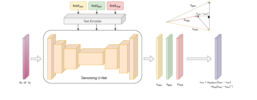
Considering the geometrical interpretation of indicates the gradient that the generative model should denoise to produce the final images, a natural solution is to find the perpendicular gradient of as the independent component of . Therefore, we now re-formulate Equation 6 and define the Perp-Neg sampler for and as
| (7) |
where denotes the vectorial inner product, and define the weights for each component, and defines the projection function to find the most correlated component of to .
Note that although the proposed perpendicular gradient sampler is applicable for both positive text prompts and negative prompts, we find in the case of concept conjunction, the positive prompts can be designed to be independent of the main prompt in an easier way, as we are creating new details in complementary to the main concept. However, in the case of concept negation, it is more frequent to observe the negative prompts have overlap with the main text prompt. Compared to the sampler in Equation 6, the most important property of the perpendicular gradient is that the component of won’t be affected by the additional prompt. Imagine the case where , using Equation 6, the denoising gradient becomes zero if we also set , which might fail the generation. However, using perpendicular gradient in Equation 7 could still preserve the main component . Below we mainly discuss the case of using perpendicular gradient sampling to handle the negative prompts and introduce Perp-Neg algorithm.
2.2.3 Perp-Neg algorithm
The above section discusses the perpendicular gradient between the main prompt and one additional prompt. Here we generalize it to a set of negative text prompts and present our Perp-Neg algorithm. We first denote and used in the previous section as and , which indicate the main positive text prompt condition and the corresponding denoising component, respectively. For any negative text prompt in the set , following equation 7, the Perp-Neg sampler is defined as
| (8) |
with , and as the weight for positive and each negative prompt. The illustration of Perp-Neg algorithm is shown in Figure 4, and the detailed algorithm is described in Algorithm 1 in Appendix.
3 2D diffusion model for 3D generation
Background: Since 2D diffusion models not only provide samples of density but also allow calculating the derivate of data density likelihood. There are several seminal works that use the latter advantage to uplift a pretrained 2D diffusion and make it a 3D generative model. The main idea behind all these methods is to optimize a 3D scene representation of an object (, NeRF [27], mesh, .) based on the likelihood that a diffusion model defines its 2D projections. To be more specific, these algorithms consist of 3 main components:
-
•
1- A 3D parametrization of the scene .
-
•
2- A differentiable renderer to create an image (or its encoded feature) from a desired camera viewpoint such that .
-
•
3- A pre-trained 2D diffusion model to obtain a proxy of where is the 2D data density and is the text prompt.
The 3D generation has been done as solving an optimization problem as follows:
where is a proxy to the negative log-likelihood of the 2D image based on the pre-trained diffusion model.
Remind the noise prediction loss in Equation 3 is a natural choice for as the training objective of the diffusion model, since it is a (weighted) evidence lower bound (ELBO) of the data density [14, 18, 31]:
| (9) |
However, direct optimization of does not provide realistic samples [31]. Therefore, Score Distillation Sampling (SDS) has been proposed as a modified version of the diffusion loss gradient , which is more robust and more computationally efficient as follows:
| (10) |
where also has been replaced with to allow text conditioning by using the classifier-free guidance [15].
Intuitively, this loss perturbs with a random amount of noise corresponding to the timestep , and estimates an update direction that follows the score function of the diffusion model to move to a higher-density region.
For the choice of , since the introduction of the seminal work DreamFusion [31], there have been several proposals [20, 25, 45]. However, since they are similar in core and our method can be applied to all of them, we continue the formulation of the paper by using the Score Distillation Sampling loss presented by DreamFusion.
3.1 The Janus problem
Since the introduction of 2D diffusion-based 3D generative models, it has been known that they suffer from the Janus (multi-faced) problem [25, 31]. This refers to a phenomenon that the learned 3D scene, instead of presenting the 3D desired output, shows multiple canonical views of an object in different directions. For instance, when the model is asked to generate a 3D sample of a person/animal, the generated object model has multiple faces of the person/animal (which is their canonical view) instead of having their back view.
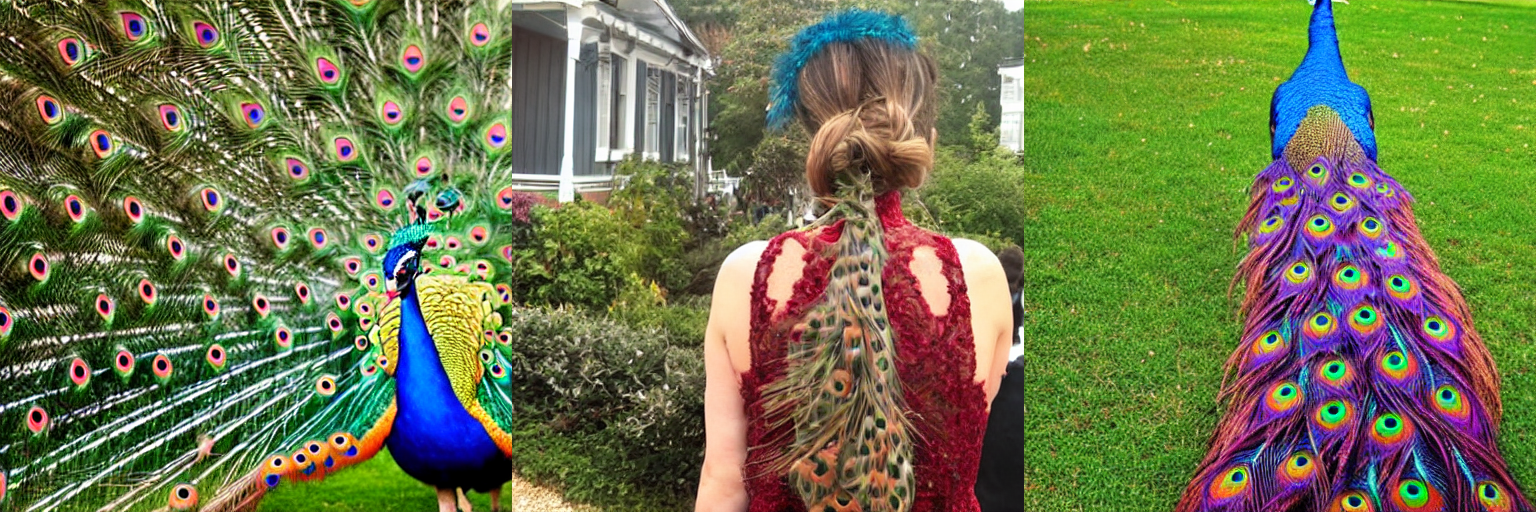
View-dependent prompting (, adding back view, side view, or overhead view with respect to the camera position to the main prompt) has been proposed as a remedy but does not fully solve the problem [32]. We believe part of the reason is that 2D Diffusion models fail to be fully conditioned on the view provided by the prompt, as also pointed out by others [25]. For instance, when the model is asked to generate the back view of a peacock, it wrongly produces the front view instead, as the front view has been more prominent in the training data the model has been trained on.
To provide an intuitive mathematical understanding of the Janus problem, we believe one of the reasons is the model fails to be properly conditioned on view . More specifically, the proxy of does not fully restrict to have zero density on areas that do not represent the viewpoint for the scene description . The main reason we think this is the case is samples of the density fail to reflect the direction of interest.
3.2 Perp-Neg to alleviate Janus problem and 2D view conditioning
In this section, we first explain how combining Perp-Neg with a unique prompting technique can enable us to accurately condition the 2D diffusion model on the desired view. Additionally, we will explore how Perp-Neg can be integrated with DreamFusion to address the Janus problem by improving the view faithfulness of the 2D model.
To begin, we demonstrate how to generate a desired statistical view using the improved model. Then, we explain the process for creating interpolations between two views To generate a specific view of an object, we use a combination of positive and negative prompts. We define , , and as the main text prompts appended by back, side, and front views, respectively. We replace simple prompts containing the view with the following set of positive and negative prompts to generate each view:
where denotes the weights for the negative prompts. Positive and negative prompts are fed into the Perp-Neg algorithm during each iteration of the diffusion model. We don’t include as a negative prompt for the generation of side/front views since most objects’ canonical view is not back. However, if the back view is more prominent for some objects, it should be included as a negative prompt. We also observed increasing the weight of the negative prompt makes the algorithm focus more on avoiding that view, acting as a pose factor.
In this subsection, we will first explain how we interpolate between the side and back views, followed by the interpolation between the front and side views. We distinguish between these two cases because the diffusion model may be biased toward generating front views, and if this assumption is not true, then the formulation needs to be adjusted accordingly.
To interpolate between the side and back views, we use the following embedding as the positive prompt:
where is the encoded text for the view and is the degree of interpolation. And for the negative prompts, we use:
such that are positive decreasing functions. The second negative prompt is chosen based on the assumption that the diffusion model is more biased towards generating samples from the front view.
For interpolation between the front and side views, the embedding for the positive would be:
and the following two negative prompts
where and both of the functions are decreasing.
Perp-Neg SDS: We employed interpolation technique in Stable DreamFusion and varied based on the related direction of 3D to 2D rendering. To be more specific, we modified the SDS loss 10 as follows:
| (11) |
such that is:
| (12) |
The unconditional term refers to , and
where refers to the text embedding of positive/negative at direction . And is the perpendical component of on . And, ’s are representative of the weights of the negative prompts at direction .
4 Experiments
In this section, we first conduct experiments on 2D cases to quantitatively demonstrate the importance of using Perp-Neg in the sampling to improve the likelihood of getting the image corresponding to the text query, which provides evidence of why our method surpasses vanilla sampling in the 3D case. Next, we show results in 3D generation.
4.1 Statistics on semantic-aligned 2D generations
To understand why Perp-Neg improves the 3D generation quality, we first explore the 2D generation of the requested view to see whether Perp-Neg produces images with fewer artifacts than the vanilla sampling method.
In the first experiment, we fix the random seeds as 0-49 to get 50 images from each text prompt. We carefully select qualified images that align with the requested text based on a series of criteria and report the percentage of accepted samples produced with Stable Diffusion, Compositional Energy-based Model (CEBM), and our Perp-Neg. Below we introduce the details of prompt design and the criteria for accepting qualified samples.
Design of prompts: We design the basic text prompts as: “A [O], [V] view.” Token [O] stands for the objects, such as panda, lion; token [V] stands for view, where we only consider “front”, “back” and “side” in our experiments. For example, we use “A panda, side view” to request the model to generate an image showing the side view of a panda. We aim to test two groups of text prompts that generate the side view and the back view of the objects, which are considered simple and complex cases, respectively. For each group, when using the negative prompts, we use the complementary view or the combination of the other two views, e.g., in the case of using the “side” view in the positive prompt, we use the “front” view in the negative prompt. Both positive and negative prompts follow the basic prompt pattern but respectively adopt positive and negative weight in the fusing stage.
Average success rate: We test each group of prompts using three objects, “panda”, “lion”, and “peacock” and only count photo-realistic generation that matches the text prompt query as a successful generation. For detailed acceptance criteria, please refer to Appendix A.2. On the side view and back view generation, in each group, we adopt 3 combinations of the complementary view into the negative prompts, e.g., for the case that side view is used in the positive prompt, we use front view, back view and both front and back view in the negative prompt. Then we count the averaged percentage of accepted successful generations, summarized in Table 1.
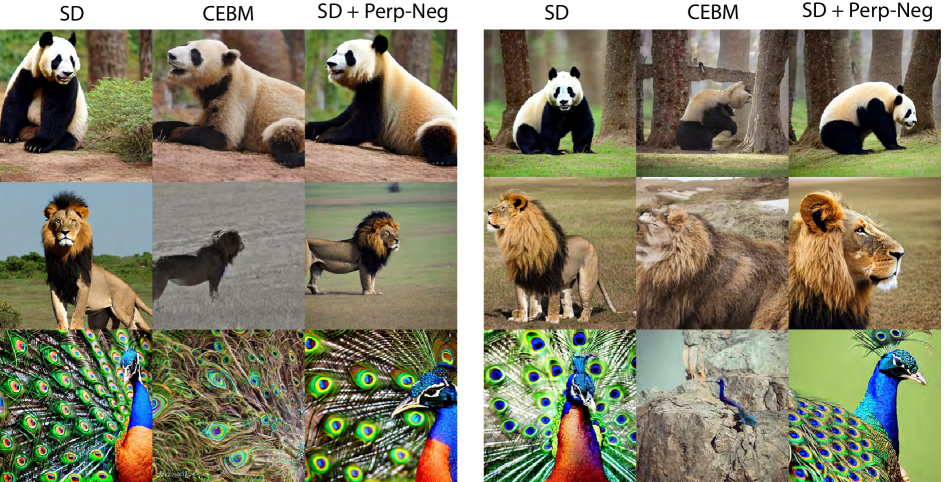
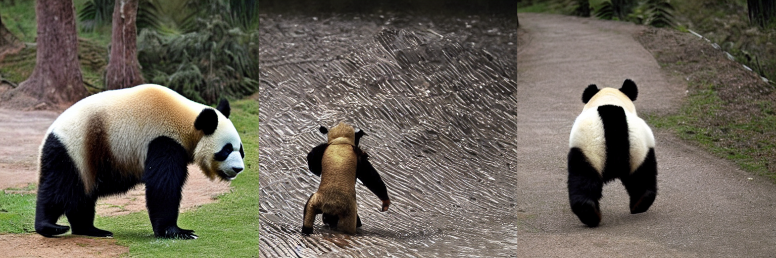
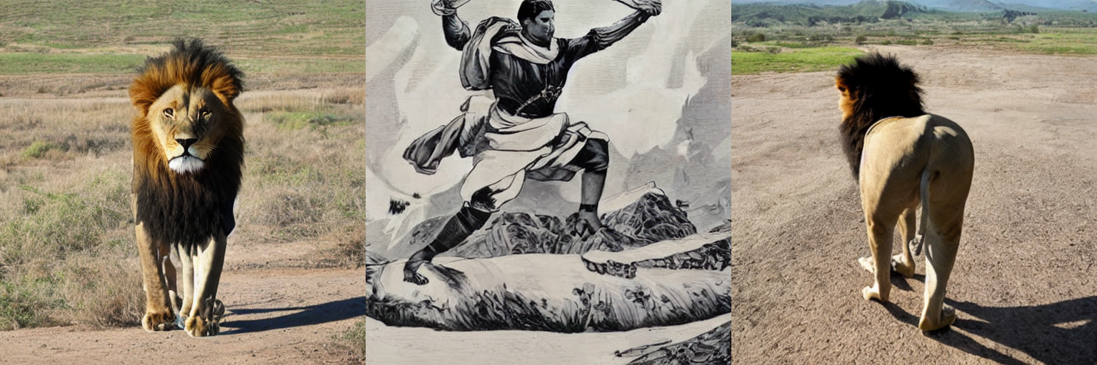
As shown, we can observe the vanilla sampling from Stable Diffusion only has 42.0% in successfully generating requested side-view images. For more difficult cases like generating the back-view images, the success rate is even lowered to 14.6%. By simply using negative prompts without considering the overlap between positive and negative prompts, CEBM fails to generate the desired view and results in a lower success rate compared to Stable Diffusion. Compared to these two types of baseline, Perp-Neg shows the effectiveness of properly using negative prompts and significantly improves the success rate by a large margin. Figure 5 shows a qualitative justification corresponding to Table 1. From the left column, we can observe without using negative prompts Stable Diffusion may generate incorrect views though requested for the back view. Although using negative prompts, CEBM does not consider the overlap between positive and negative prompts, resulting in artifacts or vanish of the content, shown in the middle column. Different than the previous two failed cases, Perp-Neg is able to properly use negative prompts to eliminate the wrong view and preserve the corresponding details of the text prompt query to achieve realistic generation well-aligned to the input text.
| Method | Side view | Back view |
|---|---|---|
| Stable Diffusion | 42.0% | 14.6% |
| CEBM | 12.7% | 2.0% |
| Perp-Neg (Ours) | 73.1% | 40.4% |
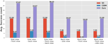
On the combination of positive and negative prompts: To explore how to combine negative prompts with positive prompt. We compute the averaged successful generation count across all tested objects and report the averaged count using different positive and negative prompt combinations in Figure 6. From the figure, it is notable that when generating the side-view images, using the back view as the negative prompt is less effective than using the front view or using the combination of both the front view and back view. Similarly, when generating back-view images, using the front view in negative prompts is also less effective, since the model is less likely to generate front-view details when conditioned on the back view, while the side view is more ambiguous to the model. This observation indicates putting ambiguous perspectives in the negative prompt could help the model avoid generating undesired images.
4.2 Perp-Neg DreamFusion
We integrated Perp-Neg with DreamFusion by using the publicly available replication of DreamFusion that utilizes Stable Diffusion as the pre-trained 2D diffusion model instead of Imagen. We replaced the SDS loss with the one provided in Equation 11. To determine the negative prompt weight functions , we used the general form of a shifted exponential decay of the form , where , , and are greater than or equal to zero. We set the parameters of the functions separately for each text prompt by generating 2D interpolation samples for 10 different random seeds and then selecting the parameters with the highest accuracy in following the conditioned view. We observed that parameters that allow better interpolation in 2D cases directly relate to the parameters that better help with the Janus problem in 3D. We also noted that if the interpolation between two views remained unchanged while varying the angle for a large range, then the 3D-generated scene was more likely to have a flat geometry from multiple views, resulting in the Janus problem. To overcome this, we perturbed the interpolation factor with random noise, calculated the interpolated text embedding and their related negative weights, and thus, the model is less likely to generate identical photos from a range of views.
To evaluate the effectiveness of the Perp-Neg in alleviating the Janus problem, we conducted our experiments using prompts that did not depict circular objects. For each prompt, we utilized the Stable DreamFusion method with and without the Perp-Neg algorithm, running 14 trials for each approach with different seeds. Our results indicate the number of successful outputs generated without a Janus problem when using the Perp-Neg algorithm: “a corgi standing” 2 times, “a westie” 5 times, “a lion” 1 time, “a Lamborghini” 5 times, “a cute pig” 0 times, and “Super Mario” 4 times. In contrast, when we ran the model without the Perp-Neg, it failed to generate any correct output except for “a Lamborghini” 4 times and “Super Mario” 2 times. These findings clearly demonstrate the advantages of utilizing the Perp-Neg in mitigating the Janus problem.
5 Conclusion
We introduce Perp-Neg, a new algorithm that enables negative prompts to overlap with positive prompts without damaging the main concept. Perp-Neg provides greater flexibility in generating images by enabling users to edit out unwanted concepts from initial generated photos. More importantly, Perp-Neg enhances prompt faithfulness by preventing the 2D diffusion model from producing biased samples from its training data and accurately representing the input prompt. This can be accomplished by feeding to Perp-Neg a sentence describing the model bias as the negative prompt to generate desired solutions. Our paper also demonstrates how Perp-Neg can properly condition the 2D diffusion model to generate views of interest rather than a canonical view. Finally, we integrate Perp-Neg’s robust view conditioning property into SDS-based text to 3D models and show how it alleviates the Janus problem.
References
- [1] Tobias Alt, Pascal Peter, and Joachim Weickert. Learning sparse masks for diffusion-based image inpainting. In Pattern Recognition and Image Analysis: 10th Iberian Conference, IbPRIA 2022, Aveiro, Portugal, May 4–6, 2022, Proceedings, pages 528–539. Springer, 2022.
- [2] Yogesh Balaji, Seungjun Nah, Xun Huang, Arash Vahdat, Jiaming Song, Karsten Kreis, Miika Aittala, Timo Aila, Samuli Laine, Bryan Catanzaro, et al. ediffi: Text-to-image diffusion models with an ensemble of expert denoisers. arXiv preprint arXiv:2211.01324, 2022.
- [3] Tim Brooks, Aleksander Holynski, and Alexei A Efros. Instructpix2pix: Learning to follow image editing instructions. arXiv preprint arXiv:2211.09800, 2022.
- [4] Duygu Ceylan, Chun-Hao Paul Huang, and Niloy J Mitra. Pix2video: Video editing using image diffusion. arXiv preprint arXiv:2303.12688, 2023.
- [5] Hila Chefer, Yuval Alaluf, Yael Vinker, Lior Wolf, and Daniel Cohen-Or. Attend-and-excite: Attention-based semantic guidance for text-to-image diffusion models. arXiv preprint arXiv:2301.13826, 2023.
- [6] Guillaume Couairon, Jakob Verbeek, Holger Schwenk, and Matthieu Cord. Diffedit: Diffusion-based semantic image editing with mask guidance. arXiv preprint arXiv:2210.11427, 2022.
- [7] Congyue Deng, Chiyu Jiang, Charles R Qi, Xinchen Yan, Yin Zhou, Leonidas Guibas, Dragomir Anguelov, et al. Nerdi: Single-view nerf synthesis with language-guided diffusion as general image priors. arXiv preprint arXiv:2212.03267, 2022.
- [8] Jacob Devlin, Ming-Wei Chang, Kenton Lee, and Kristina Toutanova. Bert: Pre-training of deep bidirectional transformers for language understanding. arXiv preprint arXiv:1810.04805, 2018.
- [9] Prafulla Dhariwal and Alexander Nichol. Diffusion models beat GANs on image synthesis. In Adv. Neural Inform. Process. Syst., 2021.
- [10] Yilun Du, Shuang Li, and Igor Mordatch. Compositional visual generation with energy based models. Advances in Neural Information Processing Systems, 33:6637–6647, 2020.
- [11] Rinon Gal, Yuval Alaluf, Yuval Atzmon, Or Patashnik, Amit H Bermano, Gal Chechik, and Daniel Cohen-Or. An image is worth one word: Personalizing text-to-image generation using textual inversion. arXiv preprint arXiv:2208.01618, 2022.
- [12] Ayaan Haque, Matthew Tancik, Alexei A Efros, Aleksander Holynski, and Angjoo Kanazawa. Instruct-nerf2nerf: Editing 3d scenes with instructions. arXiv preprint arXiv:2303.12789, 2023.
- [13] Amir Hertz, Ron Mokady, Jay Tenenbaum, Kfir Aberman, Yael Pritch, and Daniel Cohen-Or. Prompt-to-prompt image editing with cross attention control. arXiv preprint arXiv:2208.01626, 2022.
- [14] Jonathan Ho, Ajay Jain, and Pieter Abbeel. Denoising diffusion probabilistic models. NeurIPS, 2020.
- [15] Jonathan Ho and Tim Salimans. Classifier-free diffusion guidance. arXiv preprint arXiv:2207.12598, 2022.
- [16] Animesh Karnewar, Andrea Vedaldi, David Novotny, and Niloy Mitra. Holodiffusion: Training a 3d diffusion model using 2d images. arXiv preprint arXiv:2303.16509, 2023.
- [17] Bahjat Kawar, Shiran Zada, Oran Lang, Omer Tov, Huiwen Chang, Tali Dekel, Inbar Mosseri, and Michal Irani. Imagic: Text-based real image editing with diffusion models. arXiv preprint arXiv:2210.09276, 2022.
- [18] Diederik P Kingma, Tim Salimans, Ben Poole, and Jonathan Ho. Variational diffusion models. NeurIPS, 2021.
- [19] Yuheng Li, Haotian Liu, Qingyang Wu, Fangzhou Mu, Jianwei Yang, Jianfeng Gao, Chunyuan Li, and Yong Jae Lee. Gligen: Open-set grounded text-to-image generation. 2023.
- [20] Chen-Hsuan Lin, Jun Gao, Luming Tang, Towaki Takikawa, Xiaohui Zeng, Xun Huang, Karsten Kreis, Sanja Fidler, Ming-Yu Liu, and Tsung-Yi Lin. Magic3d: High-resolution text-to-3d content creation. arXiv preprint arXiv:2211.10440, 2022.
- [21] Nan Liu, Shuang Li, Yilun Du, Antonio Torralba, and Joshua B Tenenbaum. Compositional visual generation with composable diffusion models. In Computer Vision–ECCV 2022: 17th European Conference, Tel Aviv, Israel, October 23–27, 2022, Proceedings, Part XVII, pages 423–439. Springer, 2022.
- [22] Ruoshi Liu, Rundi Wu, Basile Van Hoorick, Pavel Tokmakov, Sergey Zakharov, and Carl Vondrick. Zero-1-to-3: Zero-shot one image to 3d object. arXiv preprint arXiv:2303.11328, 2023.
- [23] Andreas Lugmayr, Martin Danelljan, Andres Romero, Fisher Yu, Radu Timofte, and Luc Van Gool. Repaint: Inpainting using denoising diffusion probabilistic models. In Proceedings of the IEEE/CVF Conference on Computer Vision and Pattern Recognition, pages 11461–11471, 2022.
- [24] Chenlin Meng, Yutong He, Yang Song, Jiaming Song, Jiajun Wu, Jun-Yan Zhu, and Stefano Ermon. Sdedit: Guided image synthesis and editing with stochastic differential equations. In International Conference on Learning Representations, 2021.
- [25] Gal Metzer, Elad Richardson, Or Patashnik, Raja Giryes, and Daniel Cohen-Or. Latent-nerf for shape-guided generation of 3d shapes and textures. arXiv preprint arXiv:2211.07600, 2022.
- [26] Aryan Mikaeili, Or Perel, Daniel Cohen-Or, and Ali Mahdavi-Amiri. Sked: Sketch-guided text-based 3d editing. arXiv preprint arXiv:2303.10735, 2023.
- [27] Ben Mildenhall, Pratul P Srinivasan, Matthew Tancik, Jonathan T Barron, Ravi Ramamoorthi, and Ren Ng. Nerf: Representing scenes as neural radiance fields for view synthesis. Communications of the ACM, 65(1):99–106, 2021.
- [28] Alex Nichol, Prafulla Dhariwal, Aditya Ramesh, Pranav Shyam, Pamela Mishkin, Bob McGrew, Ilya Sutskever, and Mark Chen. Glide: Towards photorealistic image generation and editing with text-guided diffusion models. arXiv preprint arXiv:2112.10741, 2021.
- [29] Alex Nichol, Heewoo Jun, Prafulla Dhariwal, Pamela Mishkin, and Mark Chen. Point-e: A system for generating 3d point clouds from complex prompts. arXiv preprint arXiv:2212.08751, 2022.
- [30] Ryan Po and Gordon Wetzstein. Compositional 3d scene generation using locally conditioned diffusion. arXiv preprint arXiv:2303.12218, 2023.
- [31] Ben Poole, Ajay Jain, Jonathan T Barron, and Ben Mildenhall. Dreamfusion: Text-to-3d using 2d diffusion. arXiv preprint arXiv:2209.14988, 2022.
- [32] Ben Poole, Ajay Jain, Jonathan T Barron, and Ben Mildenhall. DreamFusion: Text-to-3D using 2D diffusion. arXiv preprint arXiv:2209.14988, 2022.
- [33] Colin Raffel, Noam Shazeer, Adam Roberts, Katherine Lee, Sharan Narang, Michael Matena, Yanqi Zhou, Wei Li, and Peter J Liu. Exploring the limits of transfer learning with a unified text-to-text transformer. The Journal of Machine Learning Research, 21(1):5485–5551, 2020.
- [34] Amit Raj, Srinivas Kaza, Ben Poole, Michael Niemeyer, Nataniel Ruiz, Ben Mildenhall, Shiran Zada, Kfir Aberman, Michael Rubinstein, Jonathan Barron, et al. Dreambooth3d: Subject-driven text-to-3d generation. arXiv preprint arXiv:2303.13508, 2023.
- [35] Aditya Ramesh, Prafulla Dhariwal, Alex Nichol, Casey Chu, and Mark Chen. Hierarchical text-conditional image generation with clip latents. arXiv preprint arXiv:2204.06125, 2022.
- [36] Elad Richardson, Gal Metzer, Yuval Alaluf, Raja Giryes, and Daniel Cohen-Or. Texture: Text-guided texturing of 3d shapes. arXiv preprint arXiv:2302.01721, 2023.
- [37] Robin Rombach, Andreas Blattmann, Dominik Lorenz, Patrick Esser, and Björn Ommer. High-resolution image synthesis with latent diffusion models. In IEEE Conf. Comput. Vis. Pattern Recog., 2022.
- [38] Chitwan Saharia, William Chan, Saurabh Saxena, Lala Li, Jay Whang, Emily Denton, Seyed Kamyar Seyed Ghasemipour, Burcu Karagol Ayan, S Sara Mahdavi, Rapha Gontijo Lopes, et al. Photorealistic text-to-image diffusion models with deep language understanding. arXiv preprint arXiv:2205.11487, 2022.
- [39] Jascha Sohl-Dickstein, Eric Weiss, Niru Maheswaranathan, and Surya Ganguli. Deep unsupervised learning using nonequilibrium thermodynamics. In International Conference on Machine Learning, pages 2256–2265. PMLR, 2015.
- [40] Yang Song, Jascha Sohl-Dickstein, Diederik P Kingma, Abhishek Kumar, Stefano Ermon, and Ben Poole. Score-based generative modeling through stochastic differential equations. In Int. Conf. Learn. Represent., 2021.
- [41] Xuan Su, Jiaming Song, Chenlin Meng, and Stefano Ermon. Dual diffusion implicit bridges for image-to-image translation. arXiv preprint arXiv:2203.08382, 2022.
- [42] Junshu Tang, Tengfei Wang, Bo Zhang, Ting Zhang, Ran Yi, Lizhuang Ma, and Dong Chen. Make-it-3d: High-fidelity 3d creation from a single image with diffusion prior. arXiv preprint arXiv:2303.14184, 2023.
- [43] Vishal Vinod, Tanmay Shah, and Dmitry Lagun. Teglo: High fidelity canonical texture mapping from single-view images. arXiv preprint arXiv:2303.13743, 2023.
- [44] Andrey Voynov, Qinghao Chu, Daniel Cohen-Or, and Kfir Aberman. : Extended textual conditioning in text-to-image generation. arXiv preprint arXiv:2303.09522, 2023.
- [45] Haochen Wang, Xiaodan Du, Jiahao Li, Raymond A Yeh, and Greg Shakhnarovich. Score jacobian chaining: Lifting pretrained 2d diffusion models for 3d generation. arXiv preprint arXiv:2212.00774, 2022.
- [46] Zijie J. Wang, Evan Montoya, David Munechika, Haoyang Yang, Benjamin Hoover, and Duen Horng Chau. DiffusionDB: A large-scale prompt gallery dataset for text-to-image generative models. arXiv:2210.14896 [cs], 2022.
- [47] Daniel Watson, William Chan, Ricardo Martin-Brualla, Jonathan Ho, Andrea Tagliasacchi, and Mohammad Norouzi. Novel view synthesis with diffusion models. arXiv preprint arXiv:2210.04628, 2022.
- [48] Jiahui Yu, Yuanzhong Xu, Jing Yu Koh, Thang Luong, Gunjan Baid, Zirui Wang, Vijay Vasudevan, Alexander Ku, Yinfei Yang, Burcu Karagol Ayan, et al. Scaling autoregressive models for content-rich text-to-image generation. arXiv preprint arXiv:2206.10789, 2022.
Supplementary Materials
Appendix A Experiment details
A.1 Implementation details
To clarify the difference between with/without negative prompts, and with/without Perp-Neg, we provide an illustrative depiction in Figure 8. Our Perp-Neg does not require additional training or fine-tuning, and is implemented in the sampling pipeline. A detailed implementation in each timestep is shown in Algorithm 1.

For 2D generation, we implement our Perp-Neg into Stable Diffusion v1.4 pipeline. We adopt 50 DDIM steps, and fix the guidance scale as and the positive weight , for each generation. For negative weight, the value may vary and we find generally in the range [-5, -0.5] can produce satisfactory images. In the 2D view generation experiments, we fix the negative weights to when there is only one negative prompt, and set when there are two negative prompts. The results are generated across seeds 0-49. For the interpolation between two views, we normally interpolate with stride 0.25 between 0 and 1 to have 5 images in total. Moreover, for 3D generation, we employ Perp-Neg into Stable Dreamfusion. The results of our baselines are reproduced with their open-source code***https://github.com/energy-based-model/Compositional-Visual-Generation-with-Composable-Diffusion-Models-PyTorch***https://github.com/ashawkey/stable-dreamfusion. All experiments are conducted using Pytorch 1.10 on a single NVIDIA-A5000 GPU.
A.2 Criteria for successful view generation count
Here we elaborate on the criteria for the successful generation count in our quantitative experiments in Section 4.1. We reject the image samples with the following criteria and examples are shown in Figure 9:
-
•
The images that do not show requested object(s) or view. Note that if the generated image contains multiple objects, and one of them is not positioned in the correct view, the image will still be rejected.
-
•
The images show hallucination including counterfactual details, for example, a panda has three ears.
-
•
The images have color or texture artifacts that make the images not realistic.

Appendix B Additional experiments
B.1 Case-by-case study
We further conduct case-by-case studies for the previous experiments, where we collect statistics of every tested object per view. We report the averaged acceptance rate across all possible positive and negative combinations in Table 2.
From the table, we find back view is consistently more difficult to generate than the side view. A possible explanation is that the generator may have more information about the front view from the training datasets, and the side view possesses more connection to the front view, while it requires additional knowledge to generate the corresponding back view. In terms of the objects, we find it is less likely to generate faithful images of peacock(s) in the side view, as well as peacock(s) in the back view lion in the back view, as there may have less corresponding training images in the original training datasets.
View Side Back Object Lion Panda Peacock Lion Panda Peacock SD 58.0% 44.0% 24.0% 8.0% 28.0% 8.0% CEBM 14.0% 13.3% 10.7% 0% 4.0% 2.0% Ours 80.7% 83.3% 55.3% 49.3% 34.0% 38.0%
B.2 Ablation study
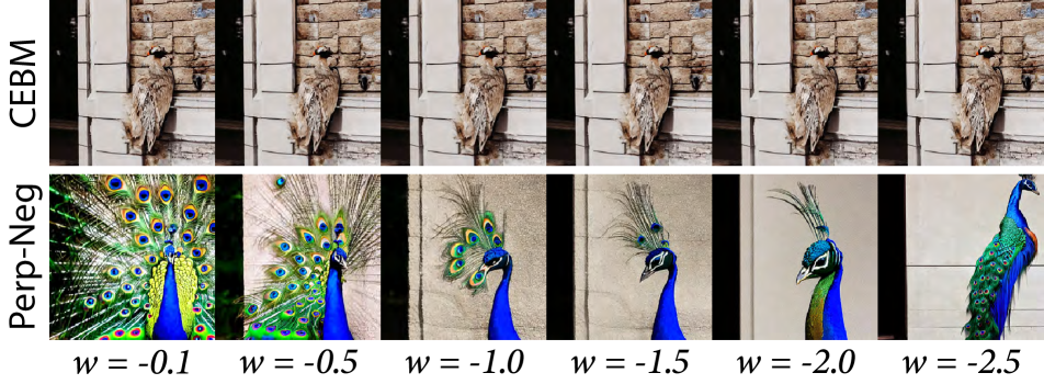
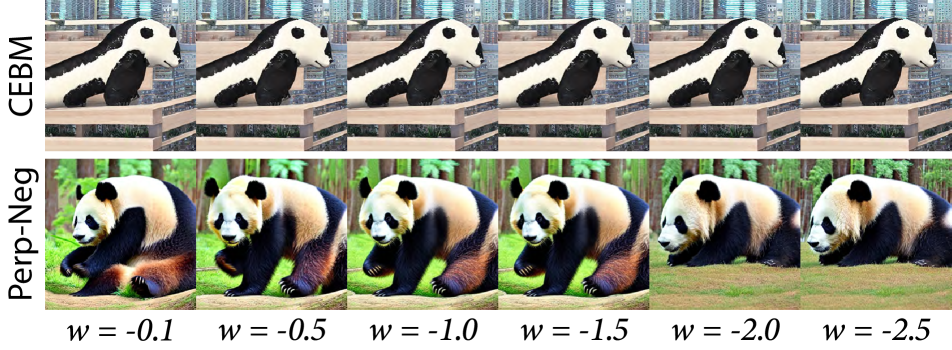
We also provide ablation studies on the effects of negative prompt weights to see how the weight affects the usage of negative attribute elimination. We show the results of generations using different negative prompt weights in Figure 10-12. We can observe for CEBM, the results are consistently not relevant to the requested text content, no matter the negative prompt weights are small or big. For Perp-Neg, we can see with larger weights, e.g., , the generated results are not positioned in the side view. As we decrease the weight, the generated image becomes more relevant to the text. This observation indicates Perp-Neg has better controllability in eliminating the negative attributes in the prompts.

B.3 Additional results
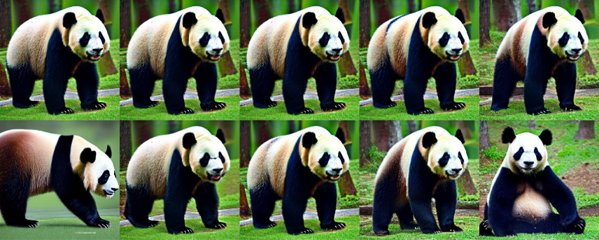
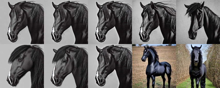
In the following, we provide additional qualitative results of 2D generation and view interpolation. And for 3D generation results, please refer to the provided video in the supplementary file.
