MRVM-NeRF: Mask-Based Pretraining for Neural Radiance Fields

Abstract

Most Neural Radiance Fields (NeRFs) have poor generalization ability, limiting their application when representing multiple scenes by a single model. To ameliorate this problem, existing methods simply condition NeRF models on image features, lacking the global understanding and modeling of the entire 3D scene. Inspired by the significant success of mask-based modeling in other research fields, we propose a masked ray and view modeling method for generalizable NeRF (MRVM-NeRF), the first attempt to incorporate mask-based pretraining into 3D implicit representations. Specifically, considering that the core of NeRFs lies in modeling 3D representations along the rays and across the views, we randomly mask a proportion of sampled points along the ray at fine stage by discarding partial information obtained from multi-viewpoints, targeting at predicting the corresponding features produced in the coarse branch. In this way, the learned prior knowledge of 3D scenes during pretraining helps the model generalize better to novel scenarios after finetuning. Extensive experiments demonstrate the superiority of our proposed MRVM-NeRF under various synthetic and real-world settings, both qualitatively and quantitatively. Our empirical studies reveal the effectiveness of our proposed innovative MRVM which is specifically designed for NeRF models.

1 Introduction

Recently Neural Radiance Fields (NeRFs) [24] have emerged as a powerful tool for 3D scene reconstruction [47, 43, 10] and generation [25, 34, 6, 7]. Though most NeRF-based methods can render striking visual effects for novel-view synthesis, they are restricted to a particular static scene, limiting their wider applications. Recent works propose Generalizable NeRF [16, 29, 44, 39, 38], aiming to share a single NeRF model across different objects.

Most of the existing generalizable NeRF methods ameliorate the limited generalization ability by conditioning NeRF on extracted image features, aggregating features from multi-view visible images into an overall 3D implicit representation. However, only incorporating 2D image features cannot help the model learn and understand 3D representations well. We pinpoint that the core of NeRF lies in understanding of the 3D representations. Motivated by the fact that masked modeling [3, 8, 41, 14] , i.e., mask-then-predict task, endows the model with better understanding of global information, we propose to incorporate mask-based modeling to pretrain NeRF models for better learning and understanding of 3D implicit representations, which further helps NeRF models generalize to various scenes. Note that the masked language modeling (MLM) [8] in natural language processing and the masked image modeling (MIM) [3, 41, 11, 14] in computer vision both mask the inputs to the model and predict the masked components in the output space, enforcing the model to learn global features from the neighbour words or pixels. Considering that NeRF models focus on representing 3D scenes, we propose an innovative masked ray and view modeling (MRVM) specially tailored for NeRF.

The essence of NeRF lies in learning and modeling 3D implicit representations along the rays and across the views. During volume rendering process, the coarse-to-fine hierarchical sampling strategy is often used, where some points are firstly sampled uniformly at coarse-stage and more additional points are then sampled during fine-stage. To tailor the masked modeling for NeRF models, we randomly mask a proportion of sampled points along the ray by discarding partial information from multiple views at fine-stage, then predict the missing information of the same point already processed by coarse-stage. Motivated by [12, 45], we perform the prediction task in the feature space. In this way, masking operation during pretraining can encourage the NeRF models to do message passing along rays and introduce interactions among viewpoints. The learnt global information about the 3D scene in such a manner helps the model generalize to novel scenes at inference time. After pretraining with our MRVM, we fine-tune the pretrained model purely with conventional pixel regression loss. With the simple yet efficient design in MRVM, our approach can be widely applicable to various generalizable NeRF models.

We conduct a series of experiments both on synthetic and real-world datasets to validate the effectiveness of our proposed MRVM-NeRF. It shows that our masked ray and view modeling can be beneficial for all the tasks in generalizable NeRF, no matter for category-agnostic generalization across multiple classes, or for category-specific generalization across objects from the same category. Quantitative and qualitative comparisons demonstrate that our proposed mask-based pretraining helps to generate visually appealing results, with precise structure and fine details.

Our contributions can be summarized as follows:

• We present a simple yet efficient mask-based pretraining scheme for generalizable NeRF, termed as MRVM-NeRF. To our best knowledge, it is the first attempt to incorporate mask-based pretraining into NeRF community.

• We propose the masked ray and view modeling (MRVM) strategy specially designed for NeRF, to help learn the 3D scene prior knowledge better.

• We perform an empirical study on the different designs for MRVM, including pretraining objectives and diverse masking hyperparameters.

Figure 1: Overview of our proposed MRVM-NeRF. To render an image viewed in a novel target viewpoint, we first cast a ray from target view into 3D scene and sample a set of points along the ray. The point is then re-projected to source views to sample local image features. We utilize transformer backbone to deal with inputs and output intermediate latent features which are then decoded to $\sigma$ and $\mathbf{c}$ for volume rendering. We also adopt coarse-to-fine sampling strategy, while the coarse and fine branch act as target and online network respectively. Our pretraining goal is to predict target latent representation from online branch in another latent space projected from NeRFormer outputs.

2 Related work

2.1 Generalizable Neural Radiance Fields

Vanilla Neural Radiance Fields (NeRFs) require per-scene optimization which can be time-consuming and computational costly. To tackle with the generalization problem across multiple scenes, the network requires an additional condition to distinguish multiple objects. Several works [16, 27, 22] extract global latent code as an additional input for neural network, while others [44, 39, 21, 37] extract a feature-map based on a CNN-like encoder and perform 3D-to-2D projection to gather features for each sampled point. These methods allow a single model handling a class of objects, and don’t require test-time optimization to generate reasonable results.

2.2 Self-Attention-Based NeRF

The multi-head self-attention (MHSA) has witnessed significant success in broad vision tasks [9, 23, 42, 46] including NeRF. IBRNet [39] firstly proposes to utilize self-attention to enhance the information interaction among sampled points on each ray. In addition, NerFormer [32] and GNT [38] use self-attention among multi-view image features to infer coordinate-aligned features. Our MRVM-NeRF  adopts the similar structure and uses masking pretraining to better facilitate message passing and scene understanding.

2.3 Mask Modeling for Pretraining

Mask-based modeling has been widely used for pretraining large models. In Natural Language Processing, Masked Language Modeling (MLM) is exploited to pretrain Bert [8] and its autoregressive variants [30, 31, 5]. In Computer Vision, Masked Image Modeling (MIM) [11, 36, 3, 41, 2] also gains significant popularity for self-supervised representation learning. Different from the aforementioned works, we perform masking and predicting operations both in a projected feature space with the inspiration from [12], which better coordinates 3D implicit representation learning for NeRF.

3 Method

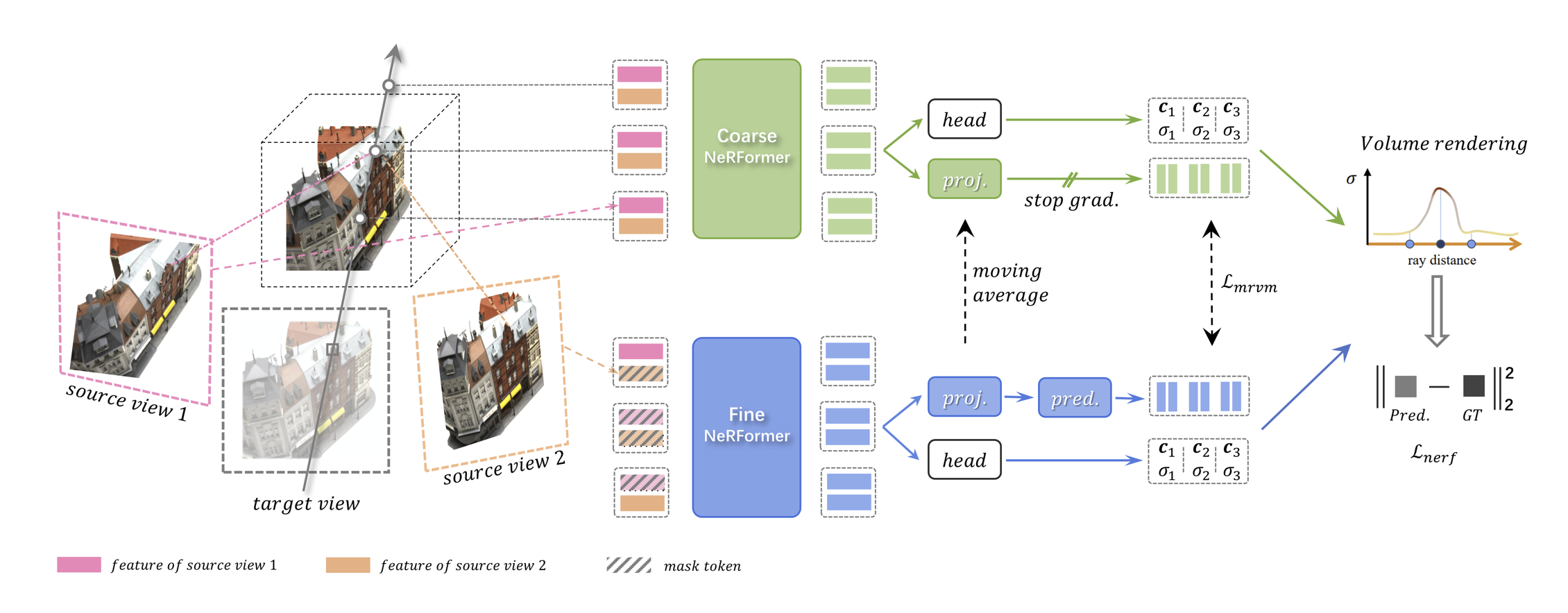
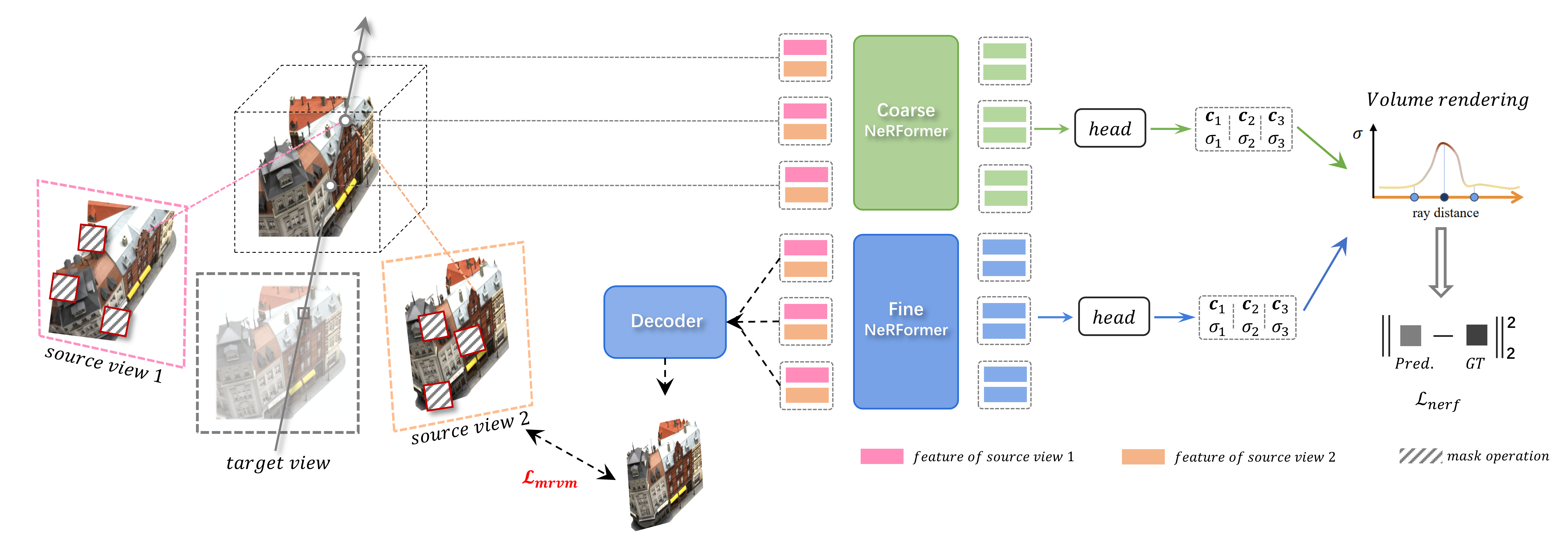
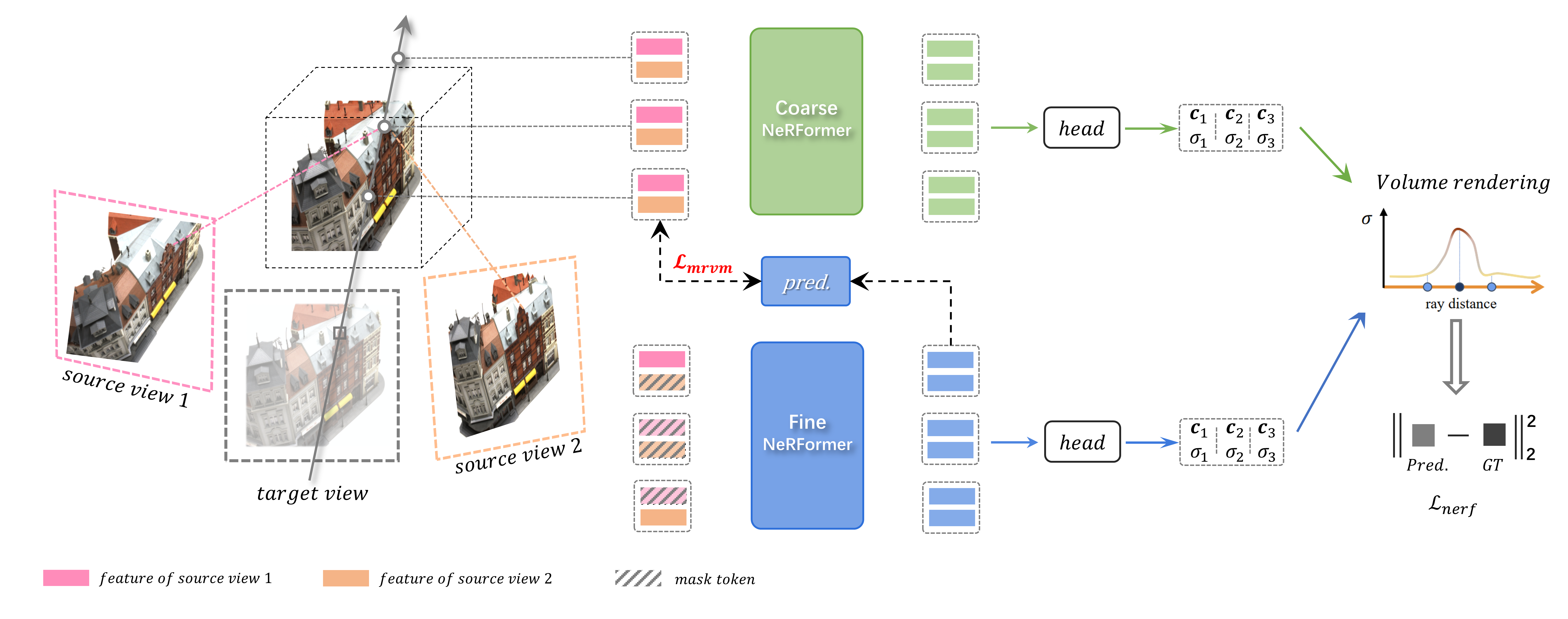
The overall pipeline of our proposed mask-based pretraining MRVM-NeRF is illustrated in Figure 1. In the following, we will firstly review our baseline NeRFormer in Section 3.1. Then we will elaborate on our proposed Masked Ray and View Modeling (MRVM) pretraining strategy in Section 3.2. The pretraining objectives and implementation details are presented in Section 3.3 and Section 3.4 respectively.

3.1 Recap NeRFormer

NeRFormer [32] is an efficient transformer-based NeRF architecture which incorporates self-attention among multi-view image features to aggregate coordinate-aligned features. In contrast, the traditional MLP-based NeRF processes each sampled 3D point independently. We figure out that the interactions between spatial locations are essential to our proposed mask-based pretraining. Therefore, we will take the effective NeRFormer as our baseline for pretraining.

NeRFormer aims to aggregate features from $S$ visible source views to generate a novel target view. $N$ different 3D points $\{\mathbf{p}_{1}$, $\mathbf{p}_{2}$ … $\mathbf{p}_{N}\}$ are firstly sampled on a ray casted from the target view. For each point $\mathbf{p}_{i}$, its corresponding multi-view RGB components $\{\mathbf{c}_{i}^{1}$, $\mathbf{c}_{i}^{2}$, …, $\mathbf{c}_{i}^{S}\}$ and image features $\{\mathbf{f}_{i}^{1}$, $\mathbf{f}_{i}^{2}$, …, $\mathbf{f}_{i}^{S}\}$ can be simply obtained by projecting $\mathbf{p}_{i}$ into $S$ source image planes and performing grid sampling. Motivated by [39, 38], we also provide the relative ray direction $\Delta\mathbf{d}_{i}^{j}$ as a cue of how close the source and target view are with each other, which can be formulated as:

$$\Delta\mathbf{d}_{i}^{j}=\mathbf{d}_{i}-\mathbf{d}_{i}^{j},\quad\quad j=1,2\cdots\cdots S,$$ (1)

where $\mathbf{d}_{i}$ and $\mathbf{d}_{i}^{j}$ represent view direction from target view and $j^{th}$ source view respectively. $\mathbf{f}_{i}^{j}$, $\mathbf{c}_{i}^{j}$ and $\Delta\mathbf{d}_{i}^{j}$ are then concatenated as a feature token $\mathbf{h}_{i}^{j}$.

To adapt NeRFormer to our mask-based pretraining strategy better, the final input token $\mathbf{z}_{i}^{j}$ is obtained by adding $\mathbf{h}_{i}^{j}$ and $\mathbf{l}_{i}$, which is the positional embedding generated from spatial location $\mathbf{x}_{i}$ and view direction $\mathbf{d}_{i}$. It can be formulated as:

$$\mathbf{z}_{i}^{j}=\mathbf{h}_{i}^{j}+\mathbf{l}_{i},\quad\quad j=1,2\cdots\cdots S.$$ (2)

$\mathbf{z}_{i}^{j}$ is then processed by NeRFormer model, stacked by several transformer blocks. Each transformer block consists of a view-attention layer followed by a ray-attention layer. Specifically, as illustrated in Figure 2, view-attention layer performs self-attention across multiple source views to generate $\hat{\mathbf{z}}_{i}^{j}$, while ray-attention layer operates information interactions among sampled points on each ray to generate $\tilde{\mathbf{z}}_{i}^{j}$, which can be represented in Equation 3 and Equation 4 respectively:

$$\{\hat{\mathbf{z}}_{i}^{1},\hat{\mathbf{z}}_{i}^{2},\cdots,\hat{\mathbf{z}}_{i}^{S}\}=View\mathchar 45\relax attn(\mathbf{z}_{i}^{1},\mathbf{z}_{i}^{2},\cdots,\mathbf{z}_{i}^{S})$$ (3)

$$\{\tilde{\mathbf{z}}_{1}^{j},\tilde{\mathbf{z}}_{2}^{j},\cdots,\tilde{\mathbf{z}}_{N}^{j}\}=Ray\mathchar 45\relax attn(\hat{\mathbf{z}}_{1}^{j},\hat{\mathbf{z}}_{2}^{j},\cdots,\hat{\mathbf{z}}_{N}^{j})$$ (4)

Afterwards, a view-weighter, parameterized by $\{w_{j}\}$, is learnt to aggregate the processed intermediate features from $S$ source views:

$$\begin{split}&\mathbf{z}_{i}=\sum_{j=1}^{S}w_{j}\tilde{\mathbf{z}}_{i}^{j},\quad s.t.\sum_{j}w_{j}=1,\quad i=1,2,\cdots,N,\end{split}$$ (5)

$\mathbf{z}_{i}$ is finally decoded into volume density $\sigma_{i}$ and color $\mathbf{c}_{i}$ for ray-marching.

3.2 Masked Ray and View Modeling

The success of MLM [8] and MIM [3] demonstrate that mask-based pretraining helps learn global and generalizable features, which is beneficial to various downstream tasks. Motivated by these works, we propose to incorporate mask-based pretraining to help train the generalizable NeRF models but with novel designs special for NeRF.

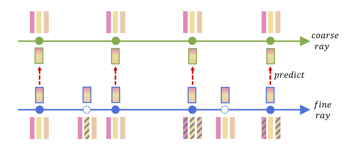
Considering that the core of NeRF lies in the 3D implicit modeling involving the processing of information along rays and across views, we propose the Masked Ray and View Modeling (MRVM), instead of masking on the inputs [8, 3, 41]. To be specific, we adopt the hierarchical sampling procedure like most NeRFs [24, 44, 38] do. The coarse stage first adopts uniform sampling, then at fine stage a few more points are sampled based on the calculated compositing weights. We perform masking operation on the points sampled at fine stage, and aim to reconstruct the corresponding target latent features produced in coarse stage from the masked fine branch.

The rationale behind our design lies in two aspects: i) only the fine branch is used during inference, masking on the fine stage can enforce the model to learn global and generalizable 3D representations which helps inference. ii) Mip-NeRF [4] claims that each of the two branches is only able to learn one scale of the scene. Inspired by this, reconstructing the features of coarse branch from masked fine branch helps to distill a disparate-scale information from coarse to fine branch.

We denote the set of points on a single ray in coarse stage as $\mathbf{P}^{c}$ and fine stage as $\mathbf{P}^{f}$, while the former is a subset of the latter:

$$\mathbf{P}^{c}={\{\mathbf{p}_{1}^{c},\mathbf{p}_{2}^{c},\dots,\mathbf{p}_{N_{c}}^{c}}\},\hphantom{dddddddddd}$$ (6)

$$\begin{split}\mathbf{P}^{f}&={\{\mathbf{p}_{1}^{f},\mathbf{p}_{2}^{f},\dots,\mathbf{p}_{N_{f}}^{f}}\}\\ &=\mathbf{P}^{c}\cup{\{\mathbf{p}_{N_{c}+1}^{f},\mathbf{p}_{N_{c}+2}^{f},\dots,\mathbf{p}_{N_{f}}^{f}}\}\\ \end{split}$$ (7)

Figure 2: NerFormer pipeline  NeRFormer consists of several view and ray attention layers followed by a view-pooling layer and a MLP-like head. It takes in image features as well as position information (location$+$direction) to predict point-wise geometry and texture attributes.

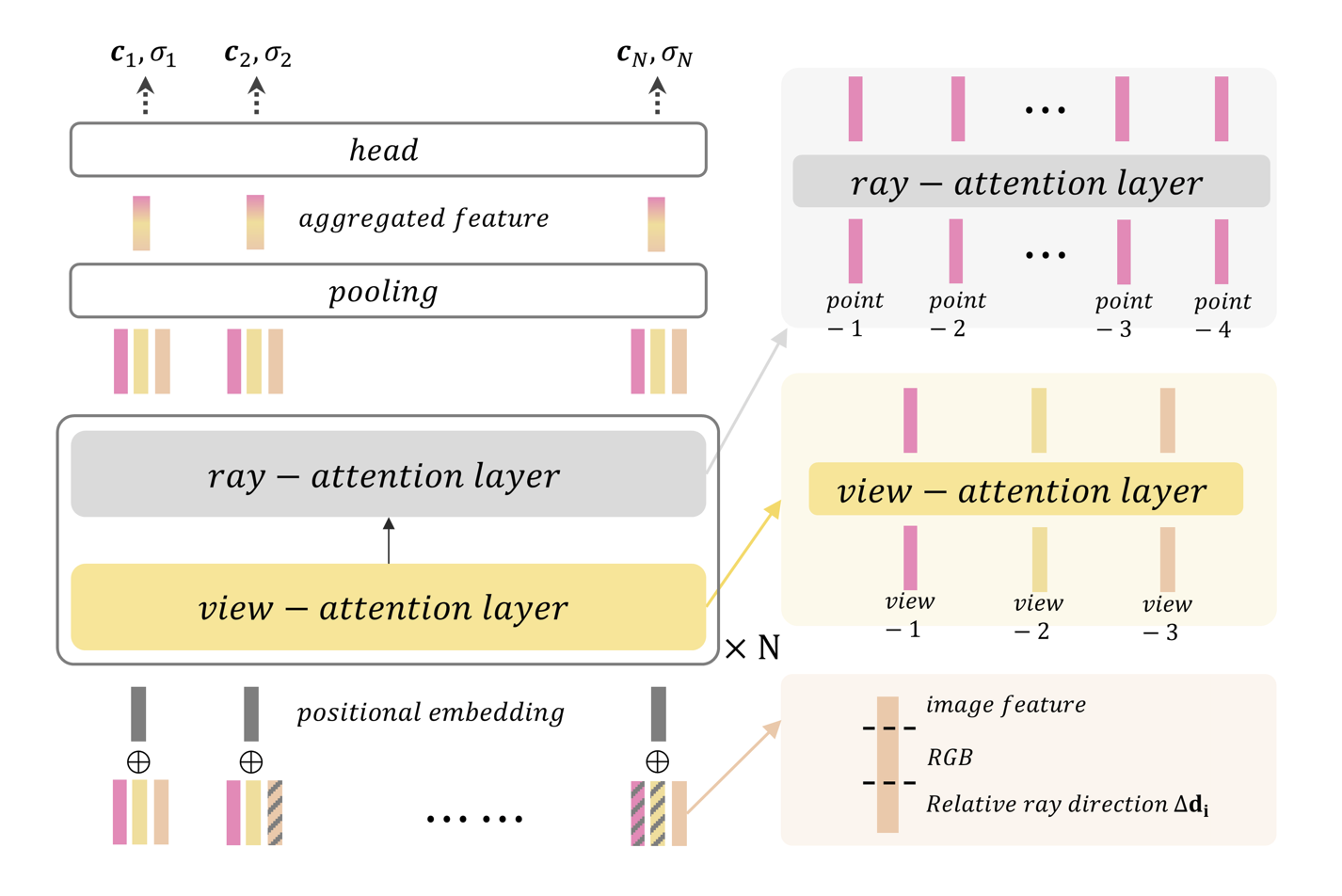
Similar to mask-based modeling in language [3] and vision [41] tasks, we use the random masking strategy for pretraining NeRF, which is illustrated in Figure 3. During pretraining, we first randomly select a set of point candidates to be masked from $\mathbf{P}^{f}$ according to the mask ratio which is a preset hyperparameter. For each selected point $\mathbf{p}_{i}$, we randomly mask $1\sim S$ different feature tokens ${\{\mathbf{h}_{i}^{j}|\ j=1\sim S}\}$ by replacing $\mathbf{h}_{i}^{j}$ with a learnable mask token. Note that the positional embedding $\mathbf{l}_{i}$ is still preserved. In this way, partial information among points along a ray is discarded and our pretraining objective is to encourage the view-attention layer and ray-attention layer to inpaint the missing information by exploiting the relative relationship with other visible points, which facilitates the model to learn some global information about the overall 3D scene thus helps to better understand it.

After masking, the multi-view features are still aggregated by Equation 5, resulting in $\mathbf{z}_{i}^{c}$ and $\mathbf{z}_{i}^{f}$ from the coarse and fine branches respectively. As shown in Figure 1, $\mathbf{z}_{i}^{c}$ and $\mathbf{z}_{i}^{f}$ are further processed for the introduction of our pretraining objective. The process can be formulated as:

$$\overline{\mathbf{z}}_{i}^{c}=Proj^{c}(\Theta,\mathbf{z}_{i}^{c}),$$ (8)

$$\overline{\mathbf{z}}_{i}^{f}=Pred^{f}(\phi,Proj^{f}(\theta,\mathbf{z}_{i}^{f})),$$ (9)

where $\Theta$, $\phi$ and $\theta$ are corresponding network parameters. The parameters of coarse-projector $\Theta$ are updated by moving average of the fine-projector $\theta$:

$$\Theta\leftarrow\tau\Theta+(1-\tau)\theta,$$ (10)

where $\tau\in[0,1]$ is the moving average decay rate. The MRVM pretraining loss is defined as a feature prediction task in the $\mathbf{\overline{z}}$ feature space:

$$\begin{split}\mathcal{L}_{mrvm}=&\frac{1}{N_{c}}\sum_{i=1}^{N_{c}}\|\frac{\overline{\mathbf{z}}_{i}^{f}}{\|\overline{\mathbf{z}}_{i}^{f}\|_{2}}-\frac{\overline{\mathbf{z}}_{i}^{c}}{\|\overline{\mathbf{z}}_{i}^{c}\|_{2}}\|_{2}^{2}\\ =&\frac{1}{N_{c}}\sum_{i=1}^{N_{c}}(2-2\frac{\overline{\mathbf{z}}_{i}^{f}}{\|\overline{\mathbf{z}}_{i}^{f}\|_{2}}\frac{\overline{\mathbf{z}}_{i}^{c}}{\|\overline{\mathbf{z}}_{i}^{c}\|_{2}}),\end{split}$$ (11)

Note that the constraint is only applied on the points appeared both in coarse and fine stages, i.e., $\mathbf{P}^{c}$.

Figure 3: Illustration of masking operation. The striped rectangles denote the masked features which are randomly selected. The solid circles represent the points sampled at coarse stage and the hollow ones correspond to extra points sampled at fine stage. The rectangles with solid box are view-aggregated features. The MRVM task aims to minimize the distance between aggregated coarse and fine features.

3.3 Training Objectives

To help the NeRF model learn better 3D implicit representations during pretraining, we also incorporate the conventional NeRF rendering task, and the aforementioned MRVM task acts as an auxiliary task to be optimized jointly.

Metrics	Methods	plane	bench	cbnt.	car	chair	disp.	lamp	spkr.	rifle	sofa	table	phone	boat	avg.
	SRN[35]	26.62	22.20	23.42	24.40	21.85	19.07	22.17	21.04	24.95	23.65	22.45	20.87	25.86	23.28
	PixelNeRF[44]	29.76	26.35	27.72	27.58	23.84	24.22	28.58	24.44	30.60	26.94	25.59	27.13	29.18	26.80
	FE-NVS[13]	30.15	27.01	28.77	27.74	24.13	24.13	28.19	24.85	30.23	27.32	26.18	27.25	28.91	27.08
	SRT[33]	31.47	28.45	30.40	28.21	24.69	24.58	28.56	25.61	30.09	28.11	27.42	28.28	29.18	27.87
	NeRFormer⋆	30.30	26.99	28.68	27.92	24.29	25.01	29.14	25.02	30.93	27.45	26.47	27.73	29.92	27.38
PSNR$\uparrow$	NeRFormer⋆+MRVM	31.69	28.46	30.21	28.96	25.45	25.92	30.34	25.97	31.87	28.68	27.88	28.82	30.67	28.58
	SRN[35]	0.901	0.837	0.831	0.897	0.814	0.744	0.801	0.779	0.913	0.851	0.828	0.811	0.898	0.849
	PixelNeRF[44]	0.947	0.911	0.910	0.942	0.858	0.867	0.913	0.855	0.968	0.908	0.898	0.922	0.939	0.910
	FE-NVS[13]	0.957	0.930	0.925	0.948	0.877	0.871	0.916	0.869	0.970	0.920	0.914	0.926	0.941	0.920
	SRT[33]	0.954	0.925	0.920	0.937	0.861	0.855	0.904	0.854	0.962	0.911	0.909	0.918	0.930	0.912
	NeRFormer⋆	0.953	0.921	0.922	0.947	0.870	0.879	0.924	0.869	0.971	0.916	0.913	0.928	0.946	0.918
SSIM$\uparrow$	NeRFormer⋆+MRVM	0.963	0.940	0.935	0.957	0.894	0.900	0.933	0.881	0.976	0.931	0.932	0.936	0.954	0.935
	SRN[35]	0.111	0.150	0.147	0.115	0.152	0.197	0.210	0.178	0.111	0.129	0.135	0.165	0.134	0.139
	PixelNeRF[44]	0.084	0.116	0.105	0.095	0.146	0.129	0.114	0.141	0.066	0.116	0.098	0.097	0.111	0.108
	FE-NVS[13]	0.061	0.080	0.076	0.085	0.103	0.105	0.091	0.116	0.048	0.081	0.071	0.080	0.094	0.082
	SRT[33]	0.050	0.068	0.058	0.062	0.085	0.087	0.082	0.096	0.045	0.066	0.055	0.059	0.079	0.066
	NeRFormer⋆	0.063	0.096	0.088	0.081	0.128	0.116	0.093	0.126	0.055	0.099	0.079	0.083	0.090	0.091
LPIPS$\downarrow$	NeRFormer⋆+MRVM	0.046	0.070	0.067	0.059	0.092	0.088	0.072	0.103	0.042	0.072	0.055	0.066	0.071	0.066

Table 1: Quantitative comparisons for category-agnostic ShapeNet-all setting. Our proposed MRVM pretraining strategy significantly helps to improve the performance compared to baseline NeRFormer^⋆, surpassing other methods without mask pretraining in all cases. Best in bold.

During training, as long as we get the generated color $c$ and its corresponding density $\sigma$ along the ray as described in Section 3.1, we use the classical volume rendering [18] to predict the pixel-wise color:

$$T_{i}=exp(-\sum_{k=1}^{i-1}\sigma_{k}\delta_{k}),$$ (12)

$$\mathbf{C}(\mathbf{r})=\sum_{i=1}^{N}T_{i}(1-exp(-\sigma_{i}\delta_{i}))\mathbf{c}_{i}.$$ (13)

The rendering supervision loss $\mathcal{L}_{nerf}$ is formulated as:

$$\begin{split}\mathcal{L}_{nerf}=\|\mathbf{C}^{*}(r)-\mathbf{C}^{c}(r)\|_{2}^{2}+\|\mathbf{C}^{*}(r)-\mathbf{C}^{f}(r)\|_{2}^{2},\end{split}$$ (14)

where $\mathbf{C}^{c}(r)$ and $\mathbf{C}^{f}(r)$ are pixels rendered by coarse and fine branch respectively, while $\mathbf{C}^{*}(r)$ is the ground truth. The overall pretraining loss is:

$$\begin{split}\mathcal{L}_{total}=\sum_{\mathbf{r}\in\mathcal{R}}(\mathcal{L}_{nerf}+\lambda\mathcal{L}_{mrvm}),\end{split}$$ (15)

where $\lambda$ is set to balance different loss terms.

After pretraining, we perform fine-tuning normally as most of works do. The projector and predictor are discarded and no masking operation is used, only the rendering loss $\mathcal{L}_{nerf}$ is used to update the model until convergence.

3.4 Implementation Details

Network details  We take the pretrained ResNet-34 [15] as the image feature extractor, whose output feature maps with four different resolutions are then concatenated and projected to $\mathbf{f}_{i}^{j}$ after interpolating to the same scale. The dimension of feature token $\mathbf{h}_{i}^{j}$ and positional embedding $\mathbf{l}_{i}$ is 128. All the attention layers have 128 channels with 4 heads. The coarse-NeRFormer and fine-NeRFormer have 4 and 5 transformer blocks respectively. The projector is a two-layer MLP which reduces the channel dimension from 128 to 64. The predictor, view-weighter and heads of NeRFormer also adopt simple MLP structure. Please refer to the Supplementary for more details.

Training details  We sample 64 points along each ray at coarse stage, and 32 extra points at fine stage. We use Adam [20] optimizer for both pretraining and fine-tuning, with learning rate set to 2e-4 and 1e-3 respectively. At pretraining stage, to improve training stability, we use a warm-up schedule increasing the learning rate linearly from 0 to 2e-4 for the first 5k steps. The moving average decay rate $\tau$ is set to 0.99. We sample 128 rays per object at pretraining while 256 rays are sampled at fine-tuning. The default mask ratio in pretraining stage is 50% unless otherwise stated. Please refer to the Supplementary for more details.

Figure 4: Visual results for category-agnostic ShapeNet-all setting. From left to right: input view image, target view images rendered by PixelNeRF [44], NeRFormer^⋆ and our MRVM-NeRF  respectively, and the ground truth image. Our proposed MRVM pretraining strategy helps to render novel view images with more plausible structure, finer details and less artifacts. More visualization results can be found in the Supplementary.

4 Experiments

We conduct a series of experiments to validate the effectiveness of our proposed MRVM pretraining strategy under both category-agnostic settings in Sec. 4.1 and category-specific settings in Sec. 4.2. We further conduct a detailed empirical study on different choices for mask-based pretraining objectives as well as mask ratios in Sec. 4.3. The limitations and future works are finally discussed in Sec. 4.4.

Baselines  We take NeRFormer [32] with some modifications detailed in Sec. 3.1 as our baseline. The baseline model is trained from scratch in an end-to-end manner using photometric loss. We denote this version (without any pretraining) as NeRFormer^⋆. Accordingly, the model with MRVM pretraining followed by fine-tuning is dubbed as NeRFormer^⋆+MRVM. We compare our method with several representative generalizable NeRF methods, e.g., SRN [35], PixelNeRF [44], FE-NVS [13], CodeNeRF [16], etc. We evaluate different models by measuring their rendered images on PSNR, SSIM [40] and LPIPS [48].

4.1 Category-agnostic View Synthesis

Settings

NMR ShapeNet [19] is a large-scale synthetic 3D dataset, containing 13 categories with 24 fixed elevation views of 64 × 64 resolution rendered for each object instance. We conduct experiments under two settings. i) In ShapeNet-all, a single model is trained across all the 13 categories and evaluated on all the classes as well. ii) In ShapeNet-unseen, the model is trained on airplane, car and chair classes while evaluated on the other 10 categories unseen in training. For both settings, during training and evaluation, a random view is selected as the input view while the remaining 23 views are used as target views.

Figure 5: Visual results for category-agnostic ShapeNet-unseen setting. With our mask-based pretraining, NeRFormer^⋆+MRVM renders images very close to the ground truth with only one observed view. On the contrary, other counterparts produce images with blurs and distortions. Please refer to the Supplementary for more visualizations.

Results on the ShapeNet-all setting

Table 1 shows the results for our model with MRVM pretraining strategy. It can be seen that our baseline NeRFormer^⋆ has already achieved comparable results to existing dominant generalizable NeRF approaches [16, 44, 35]. However, when incorporating mask-based pretraining scheme, it is further improved by +1.2 dB in PSNR, +0.02 in SSIM and -0.02 in LPIPS, respectively. SRT [33] achieves comparable result with ours in LPIPS, but it only overfits to 24 fixed viewpoints so that it cannot generate images of reasonable qualities when given an arbitrary viewpoint. This problem is pointed out in their open-sourced website, which does not exist for our models.

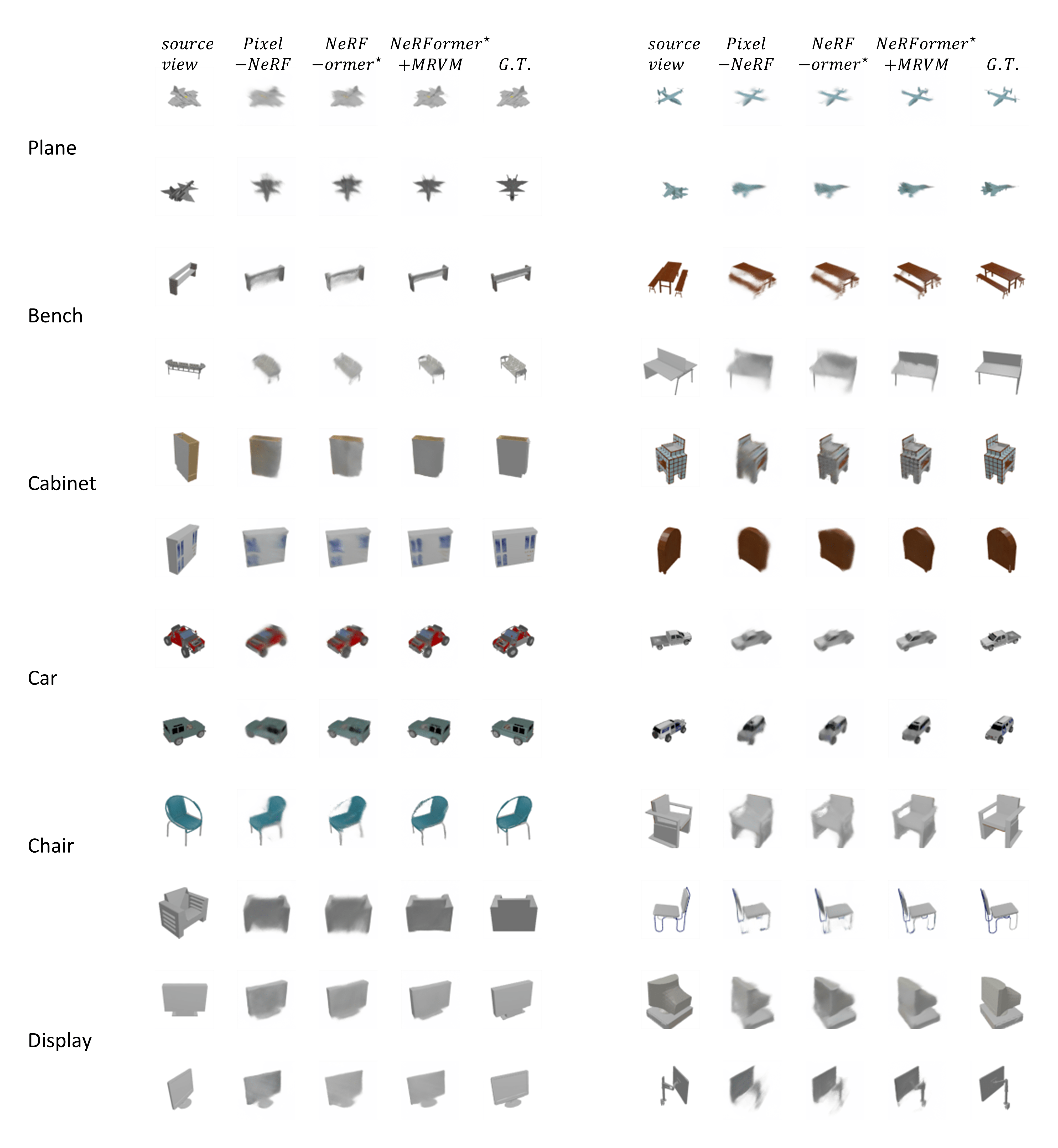
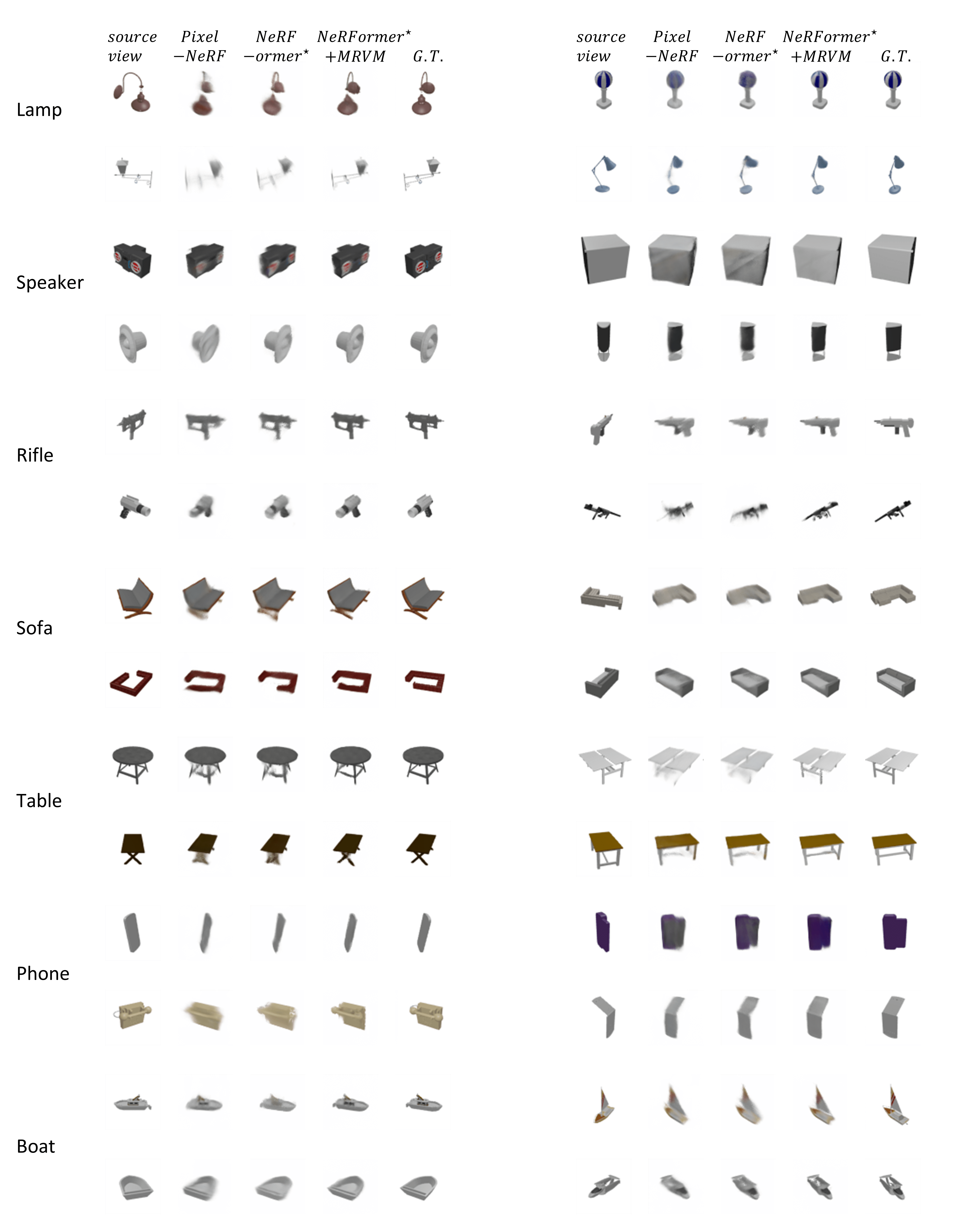
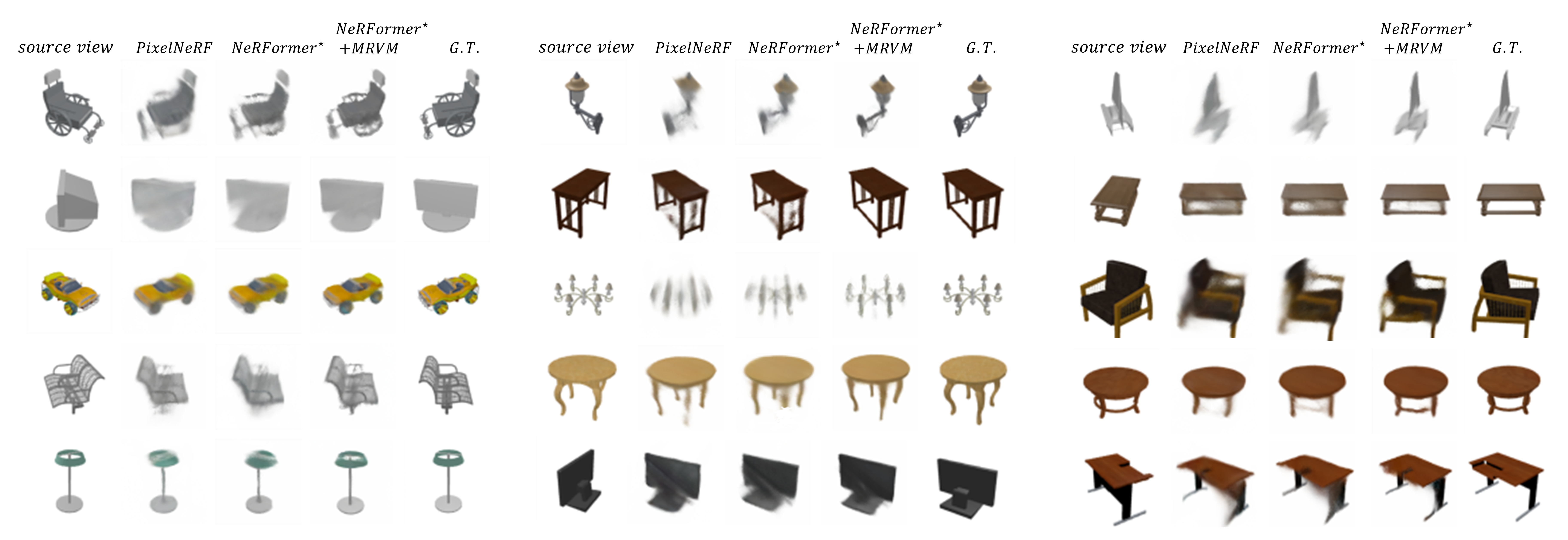
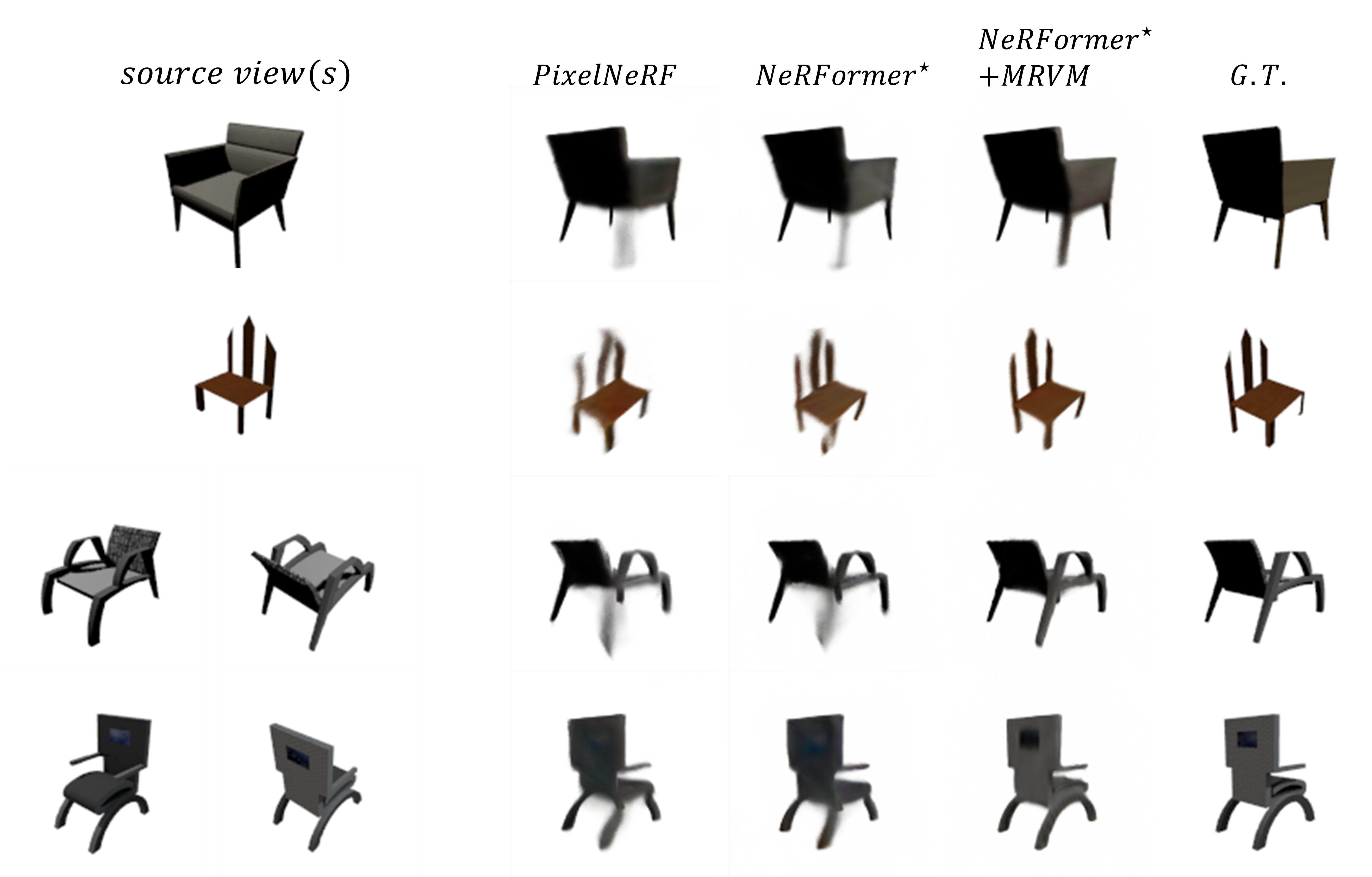
Comparisons on visualized results are shown in Figure 4. During pretraining, the MRVM-NeRF model is encouraged to predict the masked features from the rest of available ones after masked ray and view masking. This drives the model to capture prior knowledge on 3D scenes modeling. During inference, for a given object, only partial information of this object is accessible due to the limited views. The prior knowledge comes in handy for predicting the implicit representations corresponding to unseen parts so as to make the final rendered results have richer details and more precise structures. On the contrary, the methods without mask pretraining often render blurry images with artifacts and hollows, implying the lack of the predicting capacities for inferring the 3D global-scope structures and textures from limited observations.

Figure 6: Visual results for category-specific cars setting. Our mask-based pretraining helps to render images with richer details, like the patterns on the body of cars.

Figure 7: Visual results for category-specific chairs setting. Our mask-based pretraining can render images with more reasonable structures without distortions and missing parts.

Results on the ShapeNet-unseen setting

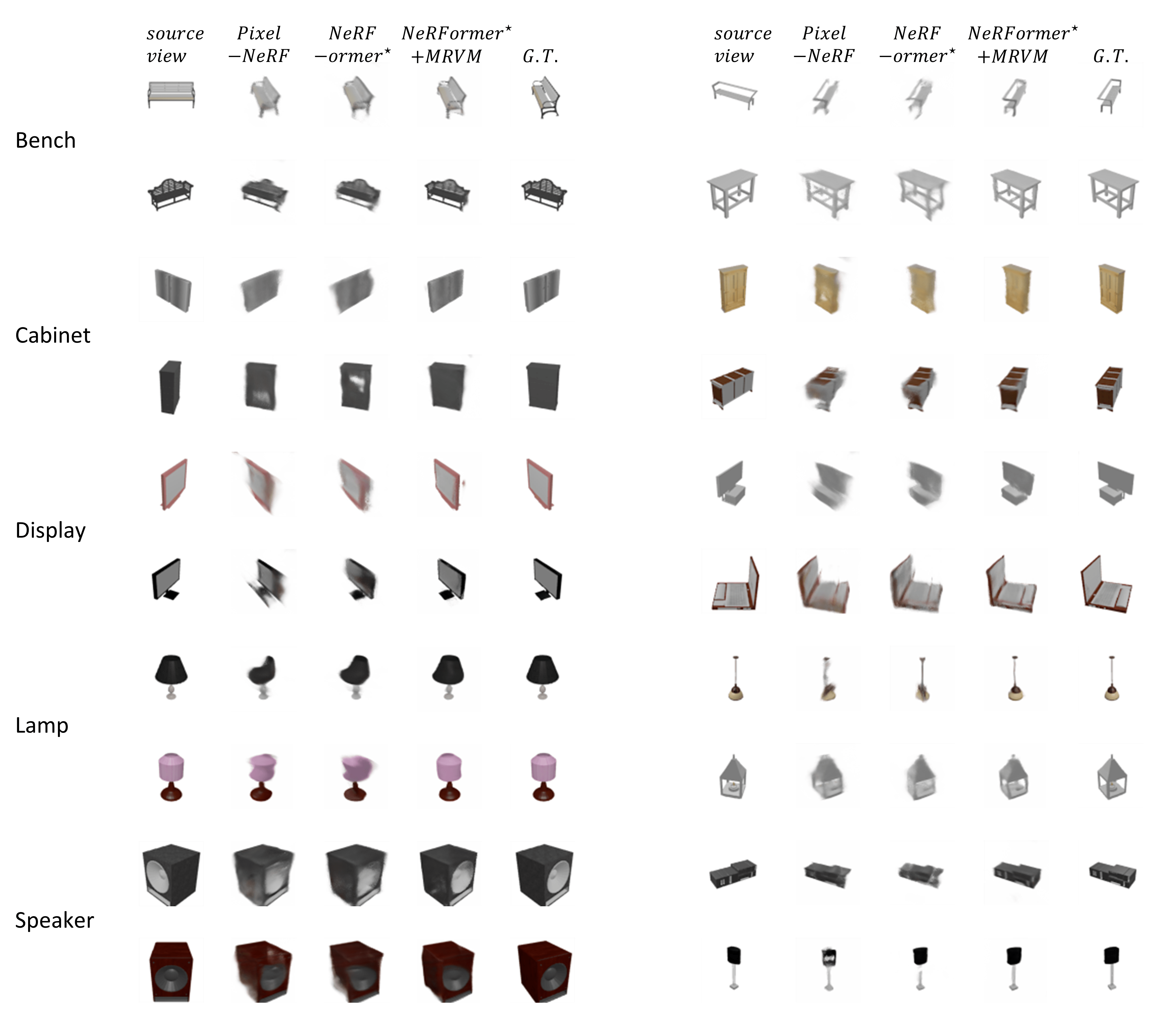
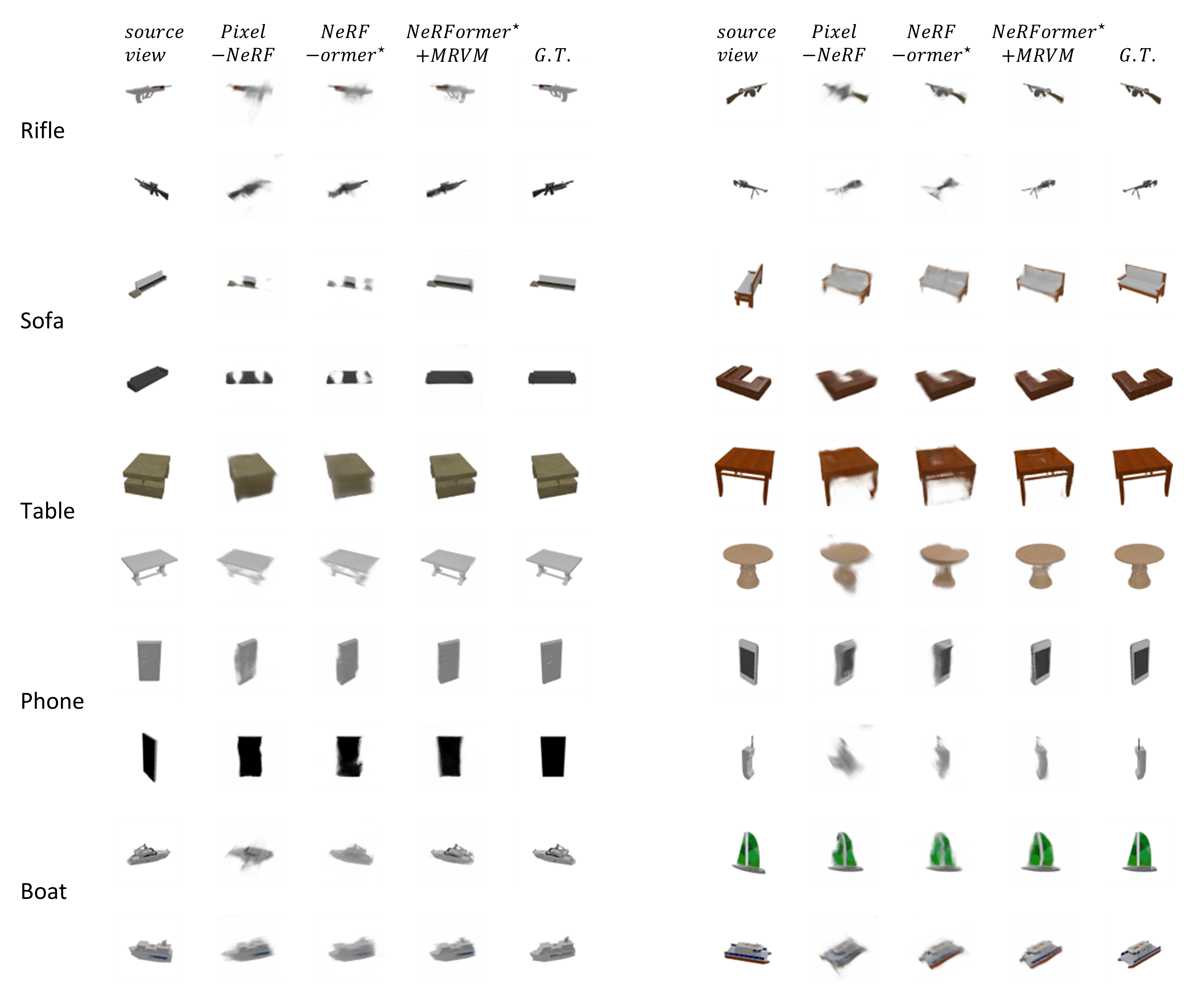
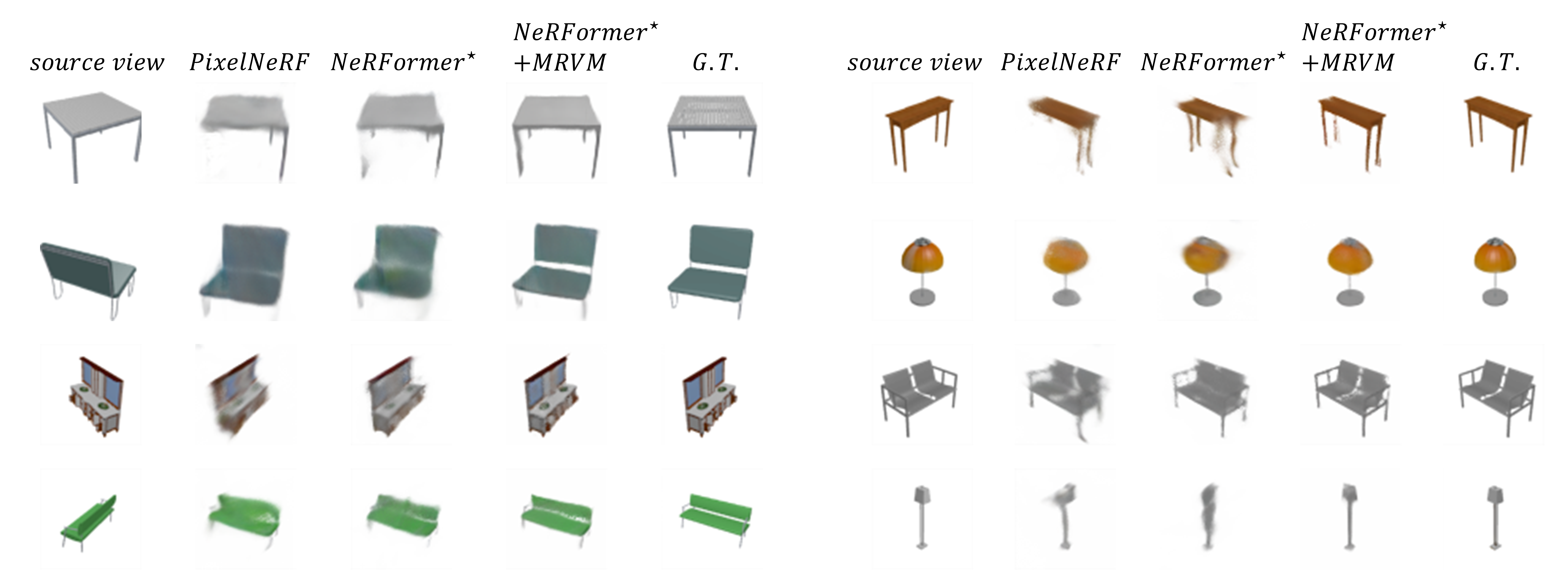
We provide quantitative and qualitative results of our proposed method in Table 2 and Figure 5 on the ShapeNet-unseen setting. This setting is more challenging than ShapeNet-all since the categories in the test set are totally unseen during training. Even under such a more difficult circumstance, our proposed pretraining strategy , i.e., masked ray and view modeling still delivers clear improvements in both numerical results and visual effects compared to the baseline model. Our NeRFormer^⋆+MRVM can not only achieve the state-of-the-art performance across all the three evaluation metrics, but also render photorealistic images that are very close to the ground truth even with only one input. This actually demonstrates that our masked ray and view modeling is useful for improving the generalizability for NeRF.

4.2 Category-specific View Synthesis

Settings  We perform one-shot and two-shot view synthesis on the chair and car classes following the protocol and dataset introduced in [35], which consists of 6591 chair and 3514 car instances with a predefined split protocol for training, testing and validation. A single model is trained for each class, with 50 views randomly sampled per object instance. During pretraining and fine-tuning process, we randomly provide 1 or 2 informative views for the network to encode. For the testing, with 251 novel views set on an Archimedean spiral, we fix 1 or 2 views of them as the inputs and perform evaluation with the rest of views. Specifically, following the common practices in [44], the 64-th view is used as the single source view setting while the 64-th and the 104-th views are used for the two-view setting.

Results  The quantitative results are reported in Table 3. The enhanced NeRFormer^⋆pretrained with our MRVM, i.e., NeRFormer^⋆+MRVM, achieves the state-of-the-art performance on most metrics, especially in SSIM and LPIPS. The CodeNeRF [16] has slightly better PSNR result in SRN-Car setting but requires a test-time optimization for latent codes, which is actually time-consuming. Our model can generate high-fidelity images without any test-time optimization.

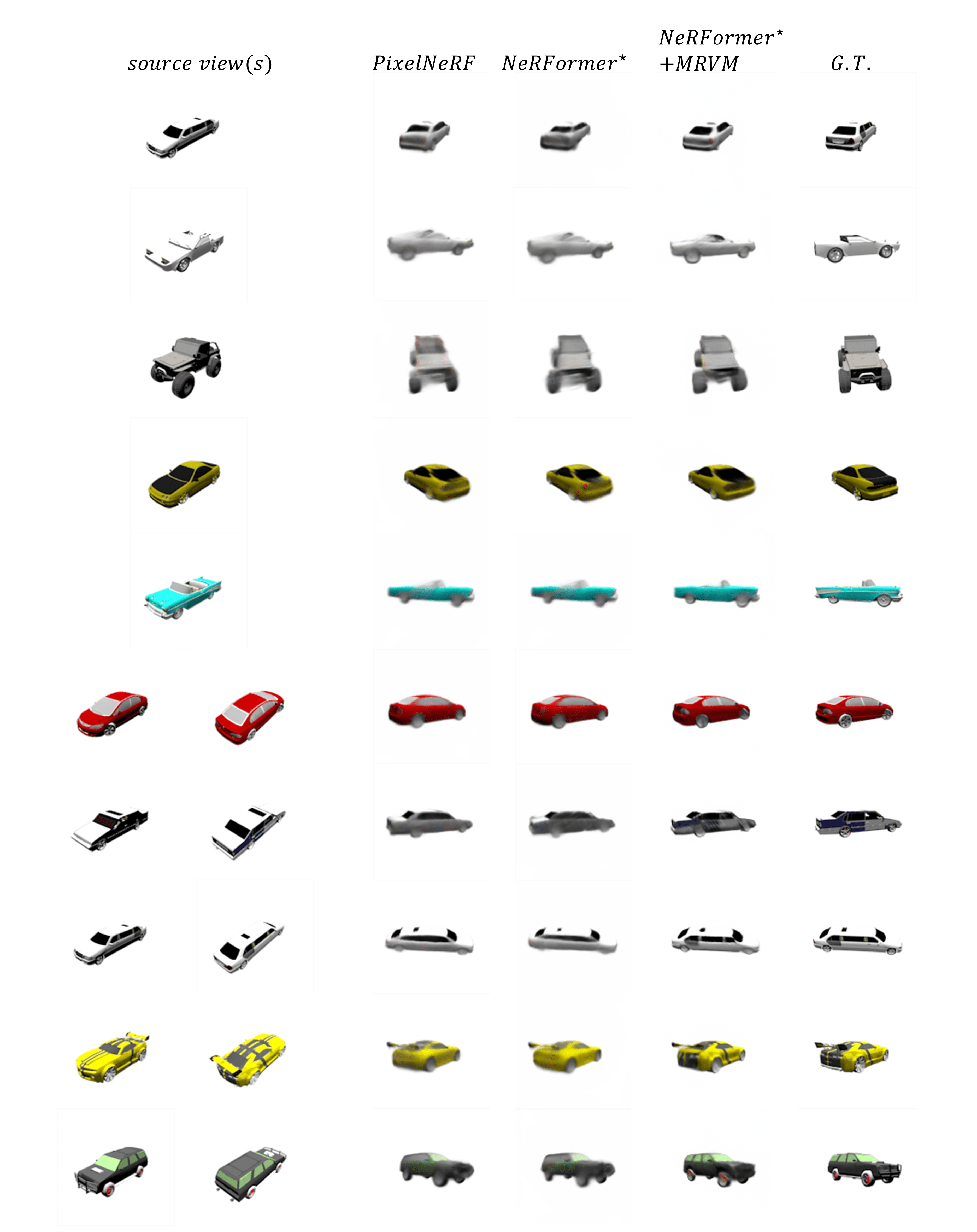
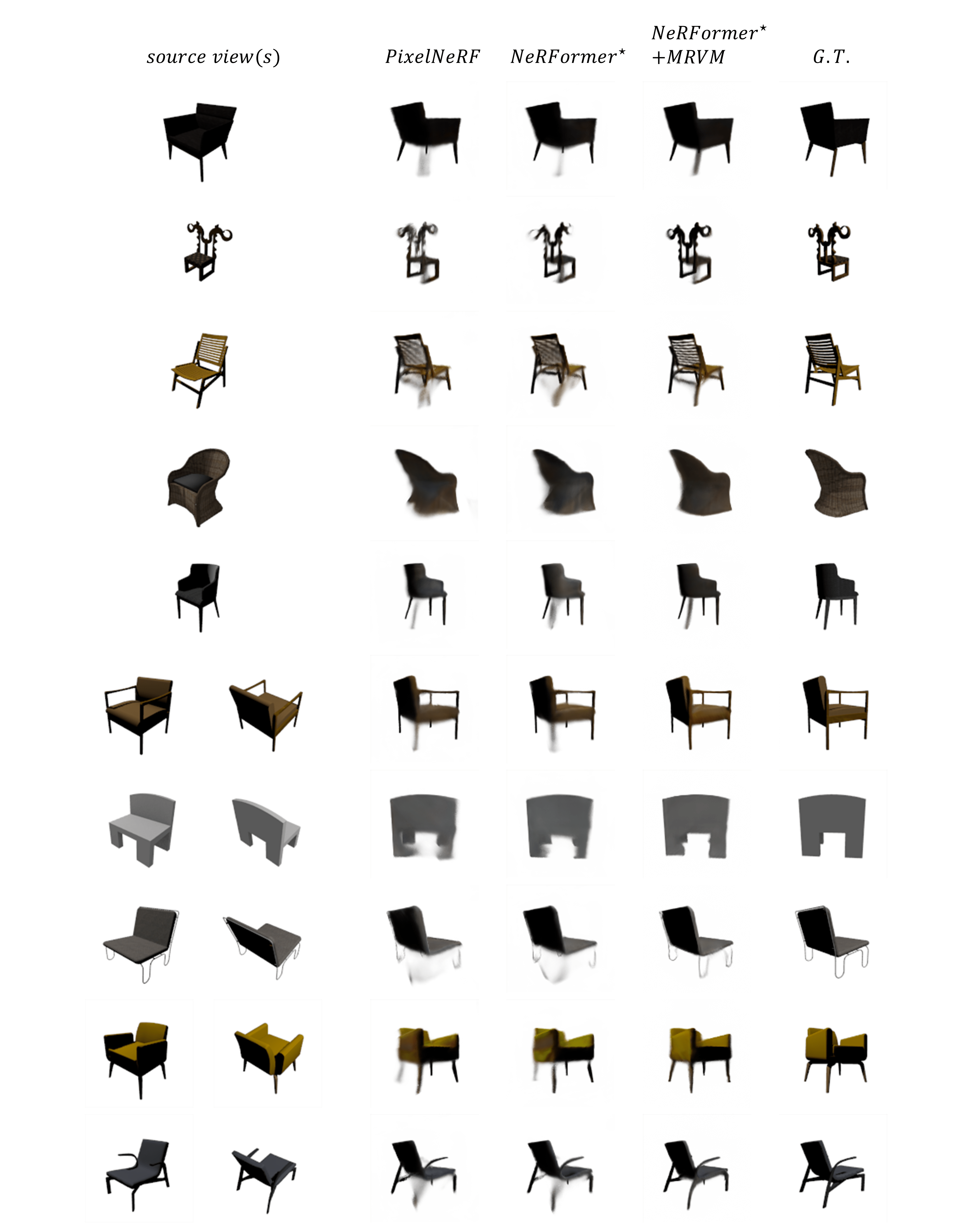
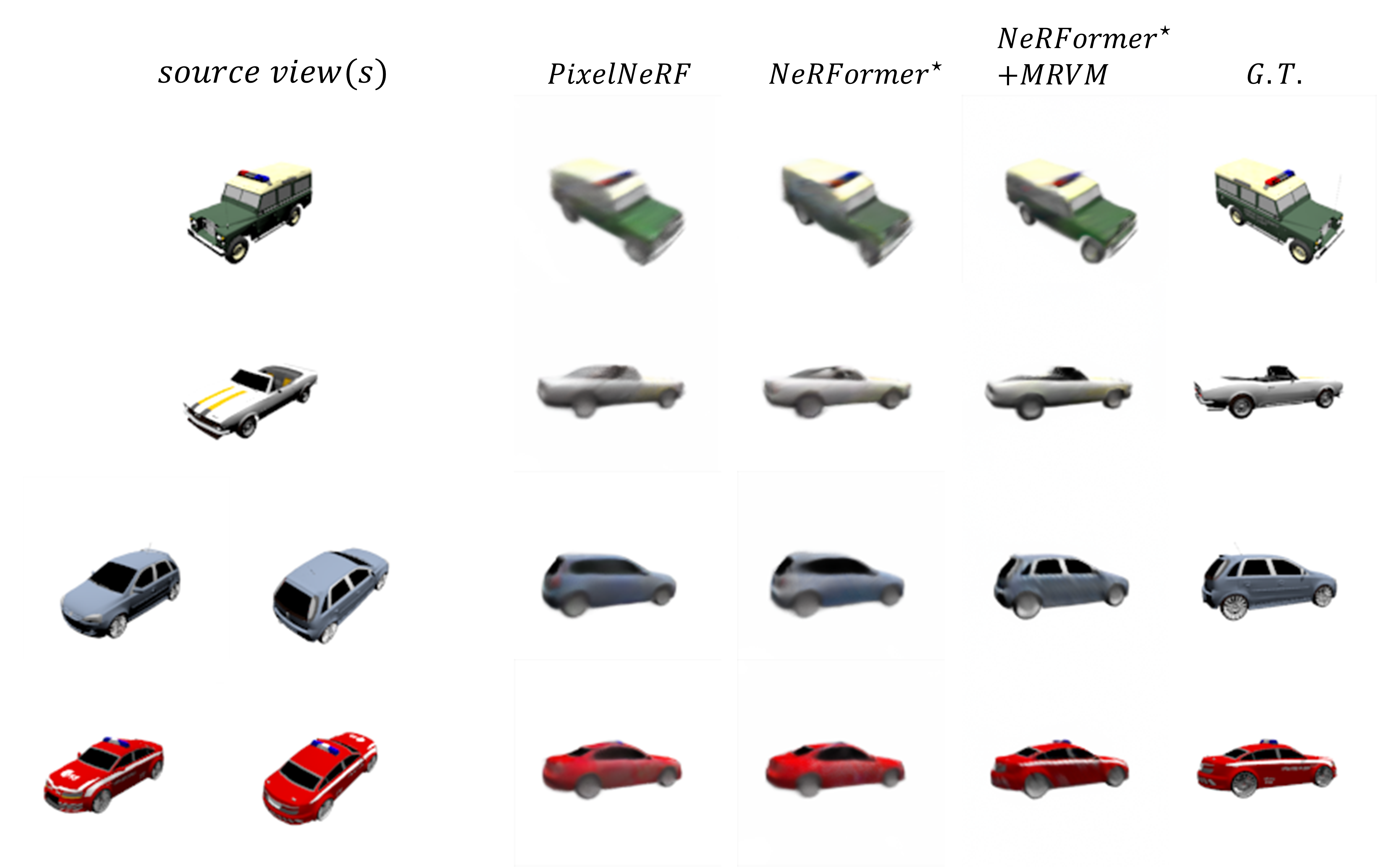
In Figure 6 and Figure 7, we provide the visualization results of SRN-Car and SRN-Chair respectively. With the help of our proposed pretraining strategy, NeRFormer^⋆+MRVM  could render more realistic images with richer details and avoid over-smoothed blurs. When the shape of testing object is rarely seen during training, NeRFormer^⋆+MRVM  has stronger capacity to predict the correct structure without distortions and aliasing.

Method	PSNR$\uparrow$	SSIM$\uparrow$	LPIPS$\downarrow$
SRN[35]	18.71	0.684	0.280
FE-NVS[13]	21.90	0.825	0.150
PixelNeRF[44]	22.71	0.825	0.182
NeRFormer⋆	22.54	0.826	0.179
NeRFormer⋆+MRVM	22.94	0.839	0.149

Table 2: Quantitative results for category-agnostic ShapeNet-unseen setting. Our proposed MRVM pretraining strategy facilitates the generalization to unseen categories. More results can be found in the Supplementary.

		1-view			2-view
		PSNR$\uparrow$	SSIM$\uparrow$	LPIPS$\downarrow$	PSNR$\uparrow$	SSIM$\uparrow$	LPIPS $\downarrow$
	SRN[35]	22.89	0.89	—	24.48	0.92	—
	CodeNeRF[16]	23.66	0.90	—	25.63	0.91	—
	FE-NVS[13]	23.21	0.92	—	25.25	0.94	—
	PixelNeRF[44]	23.72	0.91	0.128	26.20	0.94	0.080
	NeRFormer⋆	23.36	0.91	0.117	25.79	0.94	0.078
Chairs	NeRFormer⋆+MRVM	24.00	0.92	0.081	26.47	0.95	0.060
		PSNR$\uparrow$	SSIM$\uparrow$	LPIPS$\downarrow$	PSNR$\uparrow$	SSIM$\uparrow$	LPIPS $\downarrow$
	SRN[35]	22.25	0.89	—	24.84	0.92	—
	CodeNeRF[16]	23.80	0.91	—	25.71	0.93	—
	FE-NVS[13]	22.83	0.91	—	24.64	0.93	—
	PixelNeRF[44]	23.17	0.90	0.146	25.66	0.94	0.092
	NeRFormer⋆	22.98	0.90	0.125	25.12	0.93	0.088
Cars	NeRFormer⋆+MRVM	23.13	0.91	0.098	25.68	0.94	0.070

Table 3: Category-specific 1- and 2-view reconstruction results. Our final models achieve state-of-the-art performance across most evaluation metrics.

Figure 8: Visualizations on real-world DTU MVS dataset. Our masked ray and view modeling also helps to render novel views with clearer outlines on held-out scenes.

Figure 9: Ablation studies for different mask ratios. 50% works best in our experiments.

4.3 Ablation Study

Mask-based pretraining objectives  To validate the influence of different mask-based pretraining strategies, we conduct elaborated ablation studies with another 3 variants under the category-agnostic ShapeNet-all setting.

• RGB mask Following MIM [41, 11, 36, 14, 3], we randomly mask blocks of 2D input images and take an additional UNet-like decoder after the feature extractor to reconstruct the masked regions.

• Feat mask + recon-1 We take the same masking strategy as described in Sec. 3.2 but introduce an additional decoder to recover the masked latent feature ($\mathbf{h}_{i}^{j}$) from the intermediate representation ($\tilde{\mathbf{z}}_{i}^{j}$).

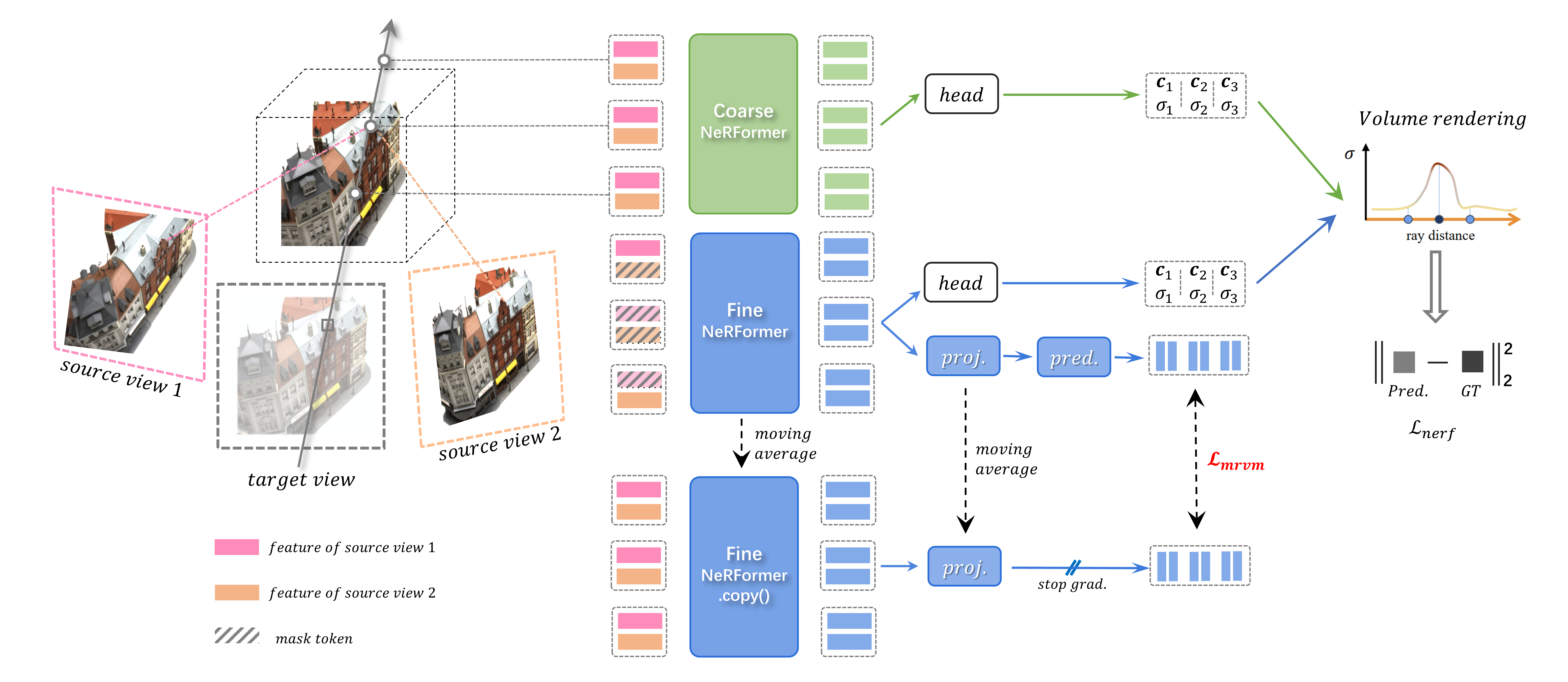
• Feat mask + recon-2 Similar to our default setting but the target network is replaced by a copy of the fine-NeRFormer, with parameters updated via moving average.

We compare the effectiveness of different objective designs for mask-based pretraining in Table 4. Though all of them can obtain more or less gains, we find out that performing masking directly in 3D space is more effective than simply masking blocks in the pixel space. Our final NeRFormer^⋆+MRVM achieves the largest improvements with the minimal additional parameters. Please refer to the Supplementary for more details about the three variants.

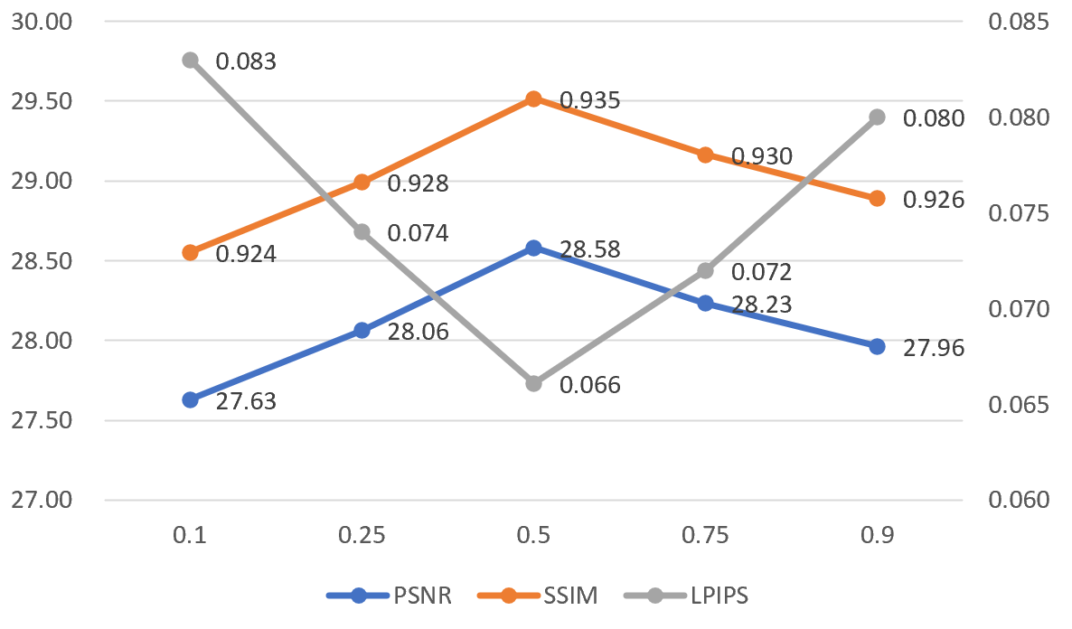
Mask ratios  As show in Figure 9, we conduct an empirical study on the mask ratio under the ShapeNet-all setting. We separately mask 10%, 25%, 50%, 75% and 90% points along the fine ray. We derive that a relatively-large mask ratio helps more, as it poses a more challenging pretraining task, forcing the model to globally understand the entire 3D scene rather than simply interpolating information from nearby points. While too large ratio will lead to too hard task, it is inappropriate for pretraining.

	PSNR$\uparrow$	SSIM$\uparrow$	LPIPS$\downarrow$	#Params(MB)
NeRFormer⋆	27.38	0.918	0.091	25.084
RGB mask	27.50	0.922	0.086	25.934
Feat mask + recon-1	28.02	0.927	0.080	25.817
Feat mask + recon-2	27.85	0.924	0.083	27.240
NeRFormer⋆+MRVM	28.58	0.935	0.066	25.151

Table 4: Ablation study for different mask-based pretraining objectives in ShapeNet-all setting.

4.4 Limitations and Future Works

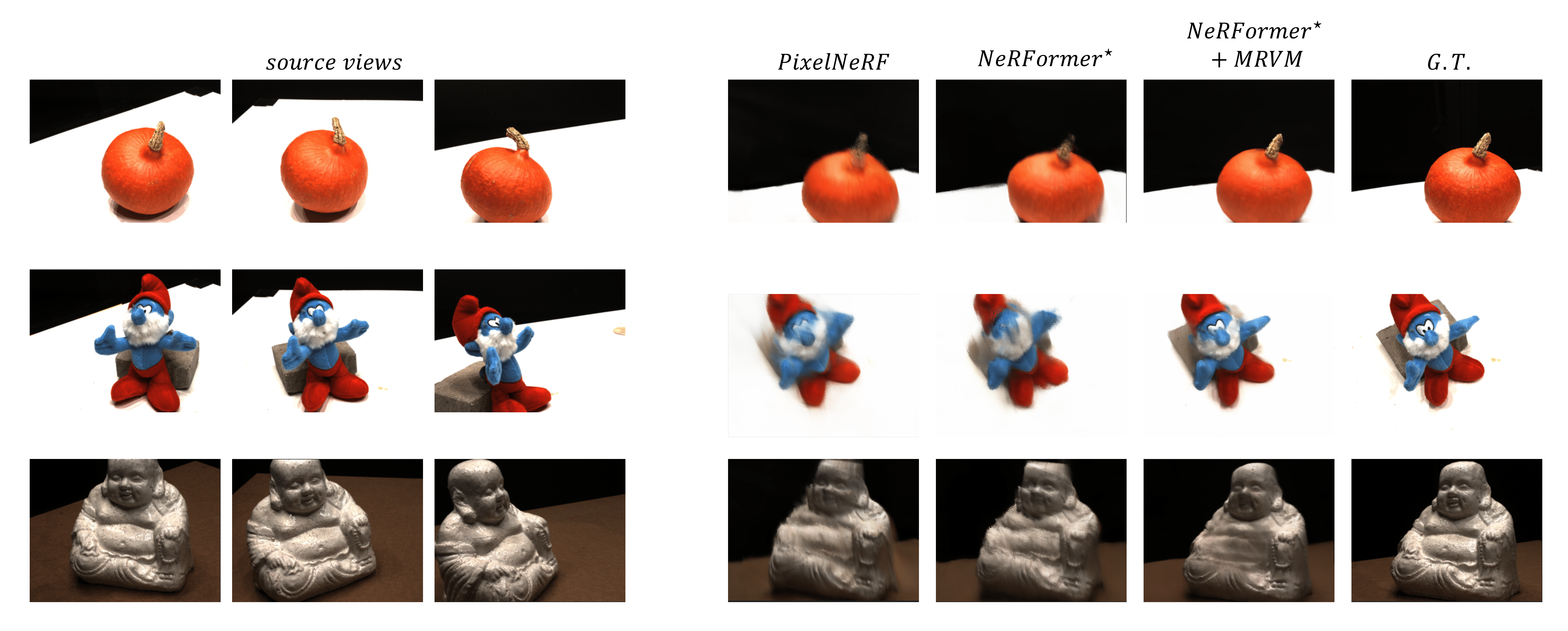
In Figure 8, we present the visualization results on real-world DTU MVS dataset [17]. We observe that the model with our proposed masked ray and view modeling could generate images with more fine-grained details on this dataset. However, the quantitative result may not be as superior as what MRVM achieves in synthetic dataset. We attribute this to the lack of sufficiently diverse scenes required for mask-based pretraining. We will explore mask-based pretraining across datasets in future works.

5 Conclusions

In this work, we propose masked ray and view modeling, the first mask-based pretraining strategy specially designed for Neural Radiance Field which can help 3D scene understanding. Extensive experiments demonstrate the capability of our MRVM for improving the generalizability of NeRF when applying to novel scenes. We hope our work will promote the development of incorporating mask-based pretraining into 3D area.

Appendix

A1. More Experimental Results

For category-agnostic ShapeNet-all setting, the detailed numerical results are presented in the main paper, while the results for our compared baselines SRN [35], PixelNeRF [44], FE-NVS [13] and SRT [33] are all obtained from their paper. The detailed category-breakdown results for SRT are provided by their authors on request. We provide additional visual results in Figure 13 and Figure 14. We randomly sample 4 object instances for each of the 13 categories in ShapeNet dataset and show comparisons to PixelNeRF [44] and our baseline NeRFormer^⋆, as done in the main paper.

For category-agnostic ShapeNet-unseen setting, we firstly provide the detailed quantitative results in Table 5 with a breakdown by categories, compared to DVR [26], SRN [35], FE-NVS [13], PixelNeRF [44] and our baseline NeRFormer^⋆. The numerical results are all obtained from corresponding papers. More visualizations could be found in Figure 15 and Figure 16. We also sample 4 object instances for each of the 10 categories in testing set.

For category-specific setting SRN-Car and SRN-Chair, the quantitative comparison on PSNR, SSIM and LPIPS could be found in the main paper. SRN [35], CodeNeRF [16] and FE-NVS [13] do not provide LPIPS number in their paper and we calculate LPIPS metric for PixelNeRF [44] using author-provided checkpoints. The additional visualizations could be found in Figure 17 and Figure 18. We use view-64 and view-64,104 as input view(s) for one-shot and two-shot cases. For each case we randomly sample 5 object instances, and show comparisons to PixelNeRF and NeRFormer^⋆.

The numerical results for real-world DTU MVS dataset [17] are presented in Table 6. At inference time, we provide 1, 3, 6, 9 informative views as input respectively, following the protocol introduced by PixelNeRF [44]. Ours NeRFormer^⋆+MRVM achieves better results in SSIM [40] and LPIPS [48], while a bit lower in PSNR. Compared to thousands of multiple scenes in synthetic ShapeNet dataset used for pretraining, DTU only has 88 training scenes and 15 testing scenes, therefore the model can be easily overfitted to the few scenes. We reckon that the lack of large-scale diverse scenes is the bottleneck to the superiority of our masked ray and view modeling. We’ll evaluate ours effectiveness once a large-scale real world dataset is available.

Metrics	Methods	bench	cbnt.	disp.	lamp	spkr.	rifle	sofa	table	phone	boat	avg.
	DVR[26]	18.37	17.19	14.33	18.48	16.09	20.28	18.62	16.20	16.84	22.43	17.72
	SRN[35]	18.71	17.04	15.06	19.26	17.06	23.12	18.76	17.35	15.66	24.97	18.71
	PixelNeRF[44]	23.79	22.85	18.09	22.76	21.22	23.68	24.62	21.65	21.05	26.55	22.71
	FE-NVS[13]	23.10	22.27	17.01	22.15	20.76	23.22	24.20	20.54	19.59	25.77	21.90
	NeRFormer⋆	23.64	22.21	17.77	23.20	20.60	24.11	24.58	21.05	21.24	27.32	22.54
PSNR$\uparrow$	NeRFormer⋆+MRVM	24.36	22.24	17.52	23.71	20.63	24.29	25.49	21.61	20.50	27.54	22.94
	DVR[26]	0.754	0.686	0.601	0.749	0.657	0.858	0.755	0.644	0.731	0.857	0.716
	SRN[35]	0.702	0.626	0.577	0.685	0.633	0.875	0.702	0.617	0.635	0.875	0.684
	PixelNeRF[44]	0.863	0.814	0.687	0.818	0.778	0.899	0.866	0.798	0.801	0.896	0.825
	FE-NVS[13]	0.865	0.819	0.686	0.822	0.785	0.902	0.872	0.792	0.796	0.898	0.825
	NeRFormer⋆	0.863	0.808	0.689	0.837	0.774	0.908	0.875	0.786	0.817	0.914	0.826
SSIM$\uparrow$	NeRFormer⋆+MRVM	0.882	0.805	0.683	0.847	0.776	0.911	0.890	0.812	0.807	0.917	0.839
	DVR[26]	0.219	0.257	0.306	0.259	0.266	0.158	0.196	0.280	0.245	0.152	0.240
	SRN[35]	0.282	0.314	0.333	0.321	0.289	0.175	0.248	0.315	0.324	0.163	0.280
	PixelNeRF[44]	0.164	0.186	0.271	0.208	0.203	0.141	0.157	0.188	0.207	0.148	0.182
	FE-NVS[13]	0.135	0.156	0.237	0.175	0.173	0.117	0.123	0.152	0.176	0.128	0.150
	NeRFormer⋆	0.161	0.195	0.263	0.203	0.205	0.129	0.142	0.199	0.192	0.119	0.179
LPIPS$\downarrow$	NeRFormer⋆+MRVM	0.126	0.175	0.250	0.173	0.185	0.112	0.114	0.154	0.186	0.107	0.149

Table 5: Detailed results of category-agnostic ShapeNet-unseen setting, with a breakdown by categories. This table is an expanding of Table 2 in the main paper.

A2. More Implementation Details

A2.1. Network Details

Encoder

We use a pretrained ResNet34 [15] provided by Pytorch [28] as the backbone to extract a feature pyramid. For a given image of size $H\times W$, the feature map has four scales:

• $64\times H/2\times W/2$

• $64\times H/4\times W/4$

• $128\times H/8\times W/8$

• $256\times H/16\times W/16$

They are later concatenated and upsampled to a feature volume of size $512\times H/2\times W/2$. After performing grid sampling, the feature vector $\mathbf{f}_{i}^{j}$ ($\in\mathbf{R}^{512}$) is concatenated with its corresponding RGB component $\mathbf{c}_{i}^{j}$ ($\in\mathbf{R}^{3}$) and relative ray direction $\Delta\mathbf{d}_{i}^{j}$ ($\in\mathbf{R}^{4}$), then projected to a feature token $\mathbf{h}_{i}^{j}$ ($\in\mathbf{R}^{128}$) by a two-layer MLP. The positional embedding $\mathbf{l}_{i}$ ($\in\mathbf{R}^{128}$) is also projected from the concatenation of location $\gamma(\mathbf{x}_{i})$ and direction $\gamma(\mathbf{d}_{i})$ after introducing positional encoding.

NeRFormer

Coarse-NeRFormer and Fine-NeRFormer have 4 and 5 blocks respectively, each block consists of a view-attention layer followed by a ray-attention layer. All the attention layers adopt classical skip connection with layer normalization [1] and set 0.1 as the dropout rate. We aggregate intermediate features from multiple views simply using a one layer view-weighter, projecting features from 128 to 1 dimension followed by a softmax operation along multiple views. It is later used to weight-average the intermediate features from multiple viewpoints. The aggregated feature is then fed into two branches. 1) Processed by a two layer MLP to decode RGB color $\mathbf{c}$ and volume density $\sigma$. 2) Projected into another latent space, where the channel dimension is 64. The projector and predictor all adopt simple two layer MLP, projecting features from 128 to 64 and 64 to 64, respectively.

A2.2. Experimental Configurations

A2.2.1. Sampling Strategies

As in vanilla NeRF [24], we adopt hierarchical sampling strategy. At coarse stage, we sample 64 points uniformly inside the sampling bounds from near to far, and sample 16 importance points based on compositing weights and 16 additional points near the surface at fine stage. The sampling bounds are set manually. They are [1.25,2.75] for SRN-Chairs, [0.8,1.8] for SRN-Cars, [1.2,4.0] for category-agnostic ShapeNet-all and ShapeNet-unseen, and [0.1,5.0] for real-world DTU.

After sampling, we use positional encoding $\gamma$ to capture high-frequency details, which can be formulated as:

$$\gamma(\mathbf{x})=(sin(2^{0}\omega\mathbf{x}),cos(2^{0}\omega\mathbf{x}),\cdots,sin(2^{L-1}\omega\mathbf{x}),cos(2^{L-1}\omega\mathbf{x})).$$ (16)

We apply positional encoding both to spatial location $\mathbf{x}$ and view direction $\mathbf{d}$. We set $L=6$ and $\omega=1.5$ for all the settings.

A2.2.2. Experimental Details

We firstly provide experimental details general to all the settings, then present contents specific to different settings.

Common configurations

As for training, we use a batch size of 16 object instances, with the number of rays sampled for each object set to 128 and 256 for pretraining and fine tuning, respectively. The coefficient $\lambda$ for loss term $\mathcal{L}_{mrvm}$ is set to 0.1 at pretraining stage. At inference time, we use the VGG network for calculating LPIPS [48] after normalizing pixel values to [-1,1]. We perform ray casting, sampling and volume rendering all in the world coordinate. All the models are implemented using Pytorch [28] framework.

For all the settings performed on synthetic datasets except for DTU, note that the images in synthetic dataset all have a blank background, we adopt two technics for better performance: i) We use bounding box sampling strategy at pretraining stage. The training rays are only sampled within the bounding box of the foreground object. In this way, it avoids the model to be too empty at initial stage. ii) We assign a white background color for those pixels sampled from the background to match the renderings in ShapeNet dataset.

Figure 10: Illustration for mask-based pretraining variant 1 — RGB mask. We mask blocks of pixels and try to recover them at pretraining.

	1-view			3-view			6-view			9-view
	PSNR$\uparrow$	SSIM$\uparrow$	LPIPS$\downarrow$	PSNR$\uparrow$	SSIM$\uparrow$	LPIPS $\downarrow$	PSNR$\uparrow$	SSIM$\uparrow$	LPIPS $\downarrow$	PSNR$\uparrow$	SSIM$\uparrow$	LPIPS $\downarrow$
PixelNeRF[44]	15.65	0.532	0.540	19.24	0.685	0.400	20.29	0.723	0.374	20.91	0.748	0.350
NeRFormer⋆	15.16	0.517	0.535	18.27	0.677	0.400	19.44	0.709	0.379	20.01	0.737	0.354
NeRFormer⋆+MRVM	15.43	0.557	0.492	18.67	0.695	0.372	19.74	0.738	0.341	20.41	0.774	0.313

Table 6: Quantitative results for real-world DTU MVS dataset. We calculate the metrics for PixelNeRF based on author-provided checkpoints. Our masked ray and view modeling achieves performance gain compared to baseline NeRFormer^⋆, and behaves better in SSIM and LPIPS compared to PixelNeRF.

Figure 11: Illustration for mask-based pretraining variant 2 — Feat mask + recon-1. We use the intermediate representation output by Fine-NeRFormer to reconstruct the masked feature tokens.

Figure 12: Illustration for mask-based pretraining variant 3 — Feat mask + recon-2. We make a copy of Fine-NeRFormer as the target branch, in place of Coarse-NeRFormer in the main paper.

Differences for synthetic datasets

For category-agnostic ShapeNet-all setting, we pretrain for 400000 iterations on 4 GTX-1080Ti, with a tight bounding box for the first 300000 iterations, then we fine tune the model without bounding box on 8 GTX-1080Ti for 800000 iterations. The two-stage training takes about 10 days.

For category-agnostic ShapeNet-unseen setting, we pretrain for 300000 iterations with bounding box on 4 GTX-1080Ti, and fine tune the model for 600000 iterations without bounding box on 8 GTX-1080Ti, which takes about 8 days.

For category-specific SRN-Car and SRN-Chair settings, we pretrain for 400000 iterations on 4 GTX-1080Ti. For the first 300000 iterations, we use 2 input views for the network to encode with a tight bounding box. For the rest of 100000 iterations and fine-tuning, the bounding box is removed and we randomly choose 1 or 2 views as input to make the model suitable for both one-shot and two-shot cases at test time. We fine tune the model on 8 GTX-1080Ti for 400000 iterations. The two-stage training takes about 7 days.

Real-world DTU

Following the protocol introduced by PixelNeRF [44], we split the dataset into 88 training scenes and 15 testing scenes. At pretraining and fine-tuning process, we randomly sample 3 input views for aggregating multi-view image features. At inference, we fix 1, 3, 6, 9 views as input views with the remaining views for testing. Specifically, view 25, 22, 28, 40, 44, 48, 0, 8, 13 are used as input, and a prefix of this list is taken if less than 9 views are used. Please refer to PixelNeRF [44] for more details.

We pretrain for 100000 iterations on 4 GTX-1080Ti, and fine tune the model for 50000 iterations on 8 GTX-1080Ti. The whole process takes about 5 days. Note that images in DTU dataset do not have a blank background, so no bounding box is used at training.

A2.3. Variants of Mask-Based Pretraining Objectives

As stated in the main paper, we conduct an elaborated ablation study on different mask-based pretraining strategies, which are illustrated in Figure 10, Figure 11 and Figure 12.

• RGB mask As shown in Figure 10, we mask blocks of pixels on input images from source views. After extracting image features by aforementioned encoder in Section A2.1. Network Details, we additionally add an UNet-like decoder to recover the input image from the feature pyramid. The loss term $\mathcal{L}_{mrvm}$ is the $\mathcal{L}_{2}$ distance between reconstructed pixels and the ground truth, the constraint is only added to masked regions. We set mask ratio to 50% and patch size to 4 at pretraining.

• Feat mask + recon-1 As illustrated in Figure 11, we also perform masking operation on sampled points along each ray. Differently, after obtaining intermediate representation $\tilde{\mathbf{z}}_{i}^{j}$ from Fine-NeRFormer, we use it to recover the masked latent feature $\mathbf{h}_{i}^{j}$ by a shallow 2-layer MLP. The loss term $\mathcal{L}_{mrvm}$ is the $\mathcal{L}_{2}$ distance between the reconstructed latent feature vector and the unmasked ground truth. We normalize the vector to unit-length before calculating the distance.

• Feat mask + recon-2 The pipeline for this variant is presented in Figure 12. Different from the architecture in the main paper, we don’t utilize Coarse-NeRFormer as target branch. On the contrary, we make a copy of the Fine-NeRFormer branch as the target network. With the gradient stopped manually, this branch is updated by moving average of the parameters from the online Fine-NeRFormer. We experimentally find that this option may cause instability at pretraining, making it inappropriate as our final proposal.

Figure 13: Category-agnostic ShapeNet-all, Part 1.

Figure 14: Category-agnostic ShapeNet-all, Part 2.

Figure 15: Category-agnostic ShapeNet-unseen, Part 1.

Figure 16: Category-agnostic ShapeNet-unseen, Part 2.

Figure 17: Category-specific SRN-Car

Figure 18: Category-specific SRN-Chair

References

- [1] Jimmy Lei Ba, Jamie Ryan Kiros, and Geoffrey E Hinton. Layer normalization. arXiv preprint arXiv:1607.06450, 2016.
- [2] Alexei Baevski, Wei-Ning Hsu, Qiantong Xu, Arun Babu, Jiatao Gu, and Michael Auli. Data2vec: A general framework for self-supervised learning in speech, vision and language. In International Conference on Machine Learning, pages 1298–1312. PMLR, 2022.
- [3] Hangbo Bao, Li Dong, and Furu Wei. Beit: Bert pre-training of image transformers. arXiv preprint arXiv:2106.08254, 2021.
- [4] Jonathan T Barron, Ben Mildenhall, Matthew Tancik, Peter Hedman, Ricardo Martin-Brualla, and Pratul P Srinivasan. Mip-nerf: A multiscale representation for anti-aliasing neural radiance fields. In Proceedings of the IEEE/CVF International Conference on Computer Vision, pages 5855–5864, 2021.
- [5] Tom Brown, Benjamin Mann, Nick Ryder, Melanie Subbiah, Jared D Kaplan, Prafulla Dhariwal, Arvind Neelakantan, Pranav Shyam, Girish Sastry, Amanda Askell, et al. Language models are few-shot learners. Advances in neural information processing systems, 33:1877–1901, 2020.
- [6] Eric R Chan, Marco Monteiro, Petr Kellnhofer, Jiajun Wu, and Gordon Wetzstein. pi-gan: Periodic implicit generative adversarial networks for 3d-aware image synthesis. In Proceedings of the IEEE/CVF conference on computer vision and pattern recognition, pages 5799–5809, 2021.
- [7] Yu Deng, Jiaolong Yang, Jianfeng Xiang, and Xin Tong. Gram: Generative radiance manifolds for 3d-aware image generation. In Proceedings of the IEEE/CVF Conference on Computer Vision and Pattern Recognition, 2022.
- [8] Jacob Devlin, Ming-Wei Chang, Kenton Lee, and Kristina Toutanova. Bert: Pre-training of deep bidirectional transformers for language understanding. arXiv preprint arXiv:1810.04805, 2018.
- [9] Alexey Dosovitskiy, Lucas Beyer, Alexander Kolesnikov, Dirk Weissenborn, Xiaohua Zhai, Thomas Unterthiner, Mostafa Dehghani, Matthias Minderer, Georg Heigold, Sylvain Gelly, et al. An image is worth 16x16 words: Transformers for image recognition at scale. arXiv preprint arXiv:2010.11929, 2020.
- [10] Sara Fridovich-Keil, Alex Yu, Matthew Tancik, Qinhong Chen, Benjamin Recht, and Angjoo Kanazawa. Plenoxels: Radiance fields without neural networks. In Proceedings of the IEEE/CVF Conference on Computer Vision and Pattern Recognition, pages 5501–5510, 2022.
- [11] Peng Gao, Teli Ma, Hongsheng Li, Jifeng Dai, and Yu Qiao. Convmae: Masked convolution meets masked autoencoders. arXiv preprint arXiv:2205.03892, 2022.
- [12] Jean-Bastien Grill, Florian Strub, Florent Altché, Corentin Tallec, Pierre Richemond, Elena Buchatskaya, Carl Doersch, Bernardo Avila Pires, Zhaohan Guo, Mohammad Gheshlaghi Azar, et al. Bootstrap your own latent-a new approach to self-supervised learning. Advances in neural information processing systems, 33:21271–21284, 2020.
- [13] Pengsheng Guo, Miguel Angel Bautista, Alex Colburn, Liang Yang, Daniel Ulbricht, Joshua M Susskind, and Qi Shan. Fast and explicit neural view synthesis. In Proceedings of the IEEE/CVF Winter Conference on Applications of Computer Vision, pages 3791–3800, 2022.
- [14] Kaiming He, Xinlei Chen, Saining Xie, Yanghao Li, Piotr Dollár, and Ross Girshick. Masked autoencoders are scalable vision learners. In Proceedings of the IEEE/CVF Conference on Computer Vision and Pattern Recognition, pages 16000–16009, 2022.
- [15] Kaiming He, Xiangyu Zhang, Shaoqing Ren, and Jian Sun. Deep residual learning for image recognition. In Proceedings of the IEEE conference on computer vision and pattern recognition, pages 770–778, 2016.
- [16] Wonbong Jang and Lourdes Agapito. Codenerf: Disentangled neural radiance fields for object categories. In Proceedings of the IEEE/CVF International Conference on Computer Vision, pages 12949–12958, 2021.
- [17] Rasmus Jensen, Anders Dahl, George Vogiatzis, Engin Tola, and Henrik Aanæs. Large scale multi-view stereopsis evaluation. In Proceedings of the IEEE conference on computer vision and pattern recognition, pages 406–413, 2014.
- [18] James T Kajiya and Brian P Von Herzen. Ray tracing volume densities. ACM SIGGRAPH computer graphics, 18(3):165–174, 1984.
- [19] Hiroharu Kato, Yoshitaka Ushiku, and Tatsuya Harada. Neural 3d mesh renderer. In Proceedings of the IEEE conference on computer vision and pattern recognition, pages 3907–3916, 2018.
- [20] Diederik P Kingma and Jimmy Ba. Adam: A method for stochastic optimization. arXiv preprint arXiv:1412.6980, 2014.
- [21] Kai-En Lin, Lin Yen-Chen, Wei-Sheng Lai, Tsung-Yi Lin, Yi-Chang Shih, and Ravi Ramamoorthi. Vision transformer for nerf-based view synthesis from a single input image. arXiv preprint arXiv:2207.05736, 2022.
- [22] Steven Liu, Xiuming Zhang, Zhoutong Zhang, Richard Zhang, Jun-Yan Zhu, and Bryan Russell. Editing conditional radiance fields. In Proceedings of the IEEE/CVF International Conference on Computer Vision, pages 5773–5783, 2021.
- [23] Ze Liu, Yutong Lin, Yue Cao, Han Hu, Yixuan Wei, Zheng Zhang, Stephen Lin, and Baining Guo. Swin transformer: Hierarchical vision transformer using shifted windows. In Proceedings of the IEEE/CVF international conference on computer vision, pages 10012–10022, 2021.
- [24] Ben Mildenhall, Pratul P Srinivasan, Matthew Tancik, Jonathan T Barron, Ravi Ramamoorthi, and Ren Ng. Nerf: Representing scenes as neural radiance fields for view synthesis. Communications of the ACM, 65(1):99–106, 2021.
- [25] Michael Niemeyer and Andreas Geiger. Giraffe: Representing scenes as compositional generative neural feature fields. In Proceedings of the IEEE/CVF Conference on Computer Vision and Pattern Recognition, pages 11453–11464, 2021.
- [26] Michael Niemeyer, Lars Mescheder, Michael Oechsle, and Andreas Geiger. Differentiable volumetric rendering: Learning implicit 3d representations without 3d supervision. In Proceedings of the IEEE/CVF Conference on Computer Vision and Pattern Recognition, pages 3504–3515, 2020.
- [27] Atsuhiro Noguchi, Xiao Sun, Stephen Lin, and Tatsuya Harada. Neural articulated radiance field. In Proceedings of the IEEE/CVF International Conference on Computer Vision, pages 5762–5772, 2021.
- [28] Adam Paszke, Sam Gross, Francisco Massa, Adam Lerer, James Bradbury, Gregory Chanan, Trevor Killeen, Zeming Lin, Natalia Gimelshein, Luca Antiga, et al. Pytorch: An imperative style, high-performance deep learning library. Advances in neural information processing systems, 32, 2019.
- [29] Sida Peng, Yuanqing Zhang, Yinghao Xu, Qianqian Wang, Qing Shuai, Hujun Bao, and Xiaowei Zhou. Neural body: Implicit neural representations with structured latent codes for novel view synthesis of dynamic humans. In Proceedings of the IEEE/CVF Conference on Computer Vision and Pattern Recognition, pages 9054–9063, 2021.
- [30] Alec Radford, Karthik Narasimhan, Tim Salimans, Ilya Sutskever, et al. Improving language understanding by generative pre-training. 2018.
- [31] Alec Radford, Jeffrey Wu, Rewon Child, David Luan, Dario Amodei, Ilya Sutskever, et al. Language models are unsupervised multitask learners. OpenAI blog, 1(8):9, 2019.
- [32] Jeremy Reizenstein, Roman Shapovalov, Philipp Henzler, Luca Sbordone, Patrick Labatut, and David Novotny. Common objects in 3d: Large-scale learning and evaluation of real-life 3d category reconstruction. In Proceedings of the IEEE/CVF International Conference on Computer Vision, pages 10901–10911, 2021.
- [33] Mehdi SM Sajjadi, Henning Meyer, Etienne Pot, Urs Bergmann, Klaus Greff, Noha Radwan, Suhani Vora, Mario Lučić, Daniel Duckworth, Alexey Dosovitskiy, et al. Scene representation transformer: Geometry-free novel view synthesis through set-latent scene representations. In Proceedings of the IEEE/CVF Conference on Computer Vision and Pattern Recognition, pages 6229–6238, 2022.
- [34] Katja Schwarz, Yiyi Liao, Michael Niemeyer, and Andreas Geiger. Graf: Generative radiance fields for 3d-aware image synthesis. Advances in Neural Information Processing Systems, 33:20154–20166, 2020.
- [35] Vincent Sitzmann, Michael Zollhöfer, and Gordon Wetzstein. Scene representation networks: Continuous 3d-structure-aware neural scene representations. Advances in Neural Information Processing Systems, 32, 2019.
- [36] Zhan Tong, Yibing Song, Jue Wang, and Limin Wang. Videomae: Masked autoencoders are data-efficient learners for self-supervised video pre-training. arXiv preprint arXiv:2203.12602, 2022.
- [37] Alex Trevithick and Bo Yang. Grf: Learning a general radiance field for 3d representation and rendering. In Proceedings of the IEEE/CVF International Conference on Computer Vision, pages 15182–15192, 2021.
- [38] Peihao Wang, Xuxi Chen, Tianlong Chen, Subhashini Venugopalan, Zhangyang Wang, et al. Is attention all nerf needs? arXiv preprint arXiv:2207.13298, 2022.
- [39] Qianqian Wang, Zhicheng Wang, Kyle Genova, Pratul P Srinivasan, Howard Zhou, Jonathan T Barron, Ricardo Martin-Brualla, Noah Snavely, and Thomas Funkhouser. Ibrnet: Learning multi-view image-based rendering. In Proceedings of the IEEE/CVF Conference on Computer Vision and Pattern Recognition, pages 4690–4699, 2021.
- [40] Zhou Wang, Alan C Bovik, Hamid R Sheikh, and Eero P Simoncelli. Image quality assessment: from error visibility to structural similarity. IEEE transactions on image processing, 13(4):600–612, 2004.
- [41] Zhenda Xie, Zheng Zhang, Yue Cao, Yutong Lin, Jianmin Bao, Zhuliang Yao, Qi Dai, and Han Hu. Simmim: A simple framework for masked image modeling. In Proceedings of the IEEE/CVF Conference on Computer Vision and Pattern Recognition, pages 9653–9663, 2022.
- [42] Xingguang Yan, Liqiang Lin, Niloy J Mitra, Dani Lischinski, Daniel Cohen-Or, and Hui Huang. Shapeformer: Transformer-based shape completion via sparse representation. In Proceedings of the IEEE/CVF Conference on Computer Vision and Pattern Recognition, pages 6239–6249, 2022.
- [43] Alex Yu, Ruilong Li, Matthew Tancik, Hao Li, Ren Ng, and Angjoo Kanazawa. Plenoctrees for real-time rendering of neural radiance fields. In Proceedings of the IEEE/CVF International Conference on Computer Vision, pages 5752–5761, 2021.
- [44] Alex Yu, Vickie Ye, Matthew Tancik, and Angjoo Kanazawa. pixelnerf: Neural radiance fields from one or few images. In Proceedings of the IEEE/CVF Conference on Computer Vision and Pattern Recognition, pages 4578–4587, 2021.
- [45] Tao Yu, Zhizheng Zhang, Cuiling Lan, Zhibo Chen, and Yan Lu. Mask-based latent reconstruction for reinforcement learning. arXiv preprint arXiv:2201.12096, 2022.
- [46] Syed Waqas Zamir, Aditya Arora, Salman Khan, Munawar Hayat, Fahad Shahbaz Khan, and Ming-Hsuan Yang. Restormer: Efficient transformer for high-resolution image restoration. In Proceedings of the IEEE/CVF Conference on Computer Vision and Pattern Recognition, pages 5728–5739, 2022.
- [47] Kai Zhang, Gernot Riegler, Noah Snavely, and Vladlen Koltun. Nerf++: Analyzing and improving neural radiance fields. arXiv preprint arXiv:2010.07492, 2020.
- [48] Richard Zhang, Phillip Isola, Alexei A Efros, Eli Shechtman, and Oliver Wang. The unreasonable effectiveness of deep features as a perceptual metric. In Proceedings of the IEEE conference on computer vision and pattern recognition, pages 586–595, 2018.