Reinforcement Learning Based Minimum State-flipped Control for the Reachability of Boolean Control Networks

Abstract

To realize reachability as well as reduce control costs of Boolean Control Networks (BCNs) with state-flipped control, a reinforcement learning based method is proposed to obtain flip kernels and the optimal policy with minimal flipping actions to realize reachability. The method proposed is model-free and of low computational complexity. In particular, Q-learning (QL), fast QL, and small memory QL are proposed to find flip kernels. Fast QL and small memory QL are two novel algorithms. Specifically, fast QL, namely, QL combined with transfer-learning and special initial states, is of higher efficiency, and small memory QL is applicable to large-scale systems. Meanwhile, we present a novel reward setting, under which the optimal policy with minimal flipping actions to realize reachability is the one of the highest returns. Then, to obtain the optimal policy, we propose QL, and fast small-memory QL for large-scale systems. Specifically, on the basis of the small memory QL mentioned before, the fast small memory QL uses a changeable reward setting to speed up the learning efficiency while ensuring the optimality of the policy. For parameter settings, we give some system properties for reference. Finally, two examples, which are a small-scale system and a large-scale one, are considered to verify the proposed method.

Reinforcement learning, model-free, Boolean control networks, reachability, state-flipped control

1 Introduction

The control of gene regulatory networks is an important issue in systems biology. The earliest modeling of gene regulatory networks dates back to 1969 when Kauffman[1] proposed Boolean networks (BNs). A BN contains several Boolean variables, each of which takes a value of ``0” or ``1” to indicate whether the gene is transcribed or not. Gene regulatory networks tend to have exogenous inputs. To better describe the behaviors of gene regulatory networks, BNs were extended to BCNs, namely, BNs with control inputs.

State-flipped control is a novel control method. It can be applied to a subset of nodes in BCNs, turning each node from ``1” to ``0”, or from ``0” to ``1”. Compare with the existing control methods such as pinning control, the advantage of state-flipped control is that it can achieve the control goal with little damage to the system. Rafimanzelat et al. [2] first proposed the concept of state-flipped control. Then, fundamental problems of BCNs with state-flipped control have been carried out [3, 4, 5]. However, [2, 3, 4, 5] only consider one-time flipping, where some control problems are difficult to implement. Liu et al. [6] proposed a more general state-flipped control, namely, flipping each node more than once. This opened a new chapter in research related to state-flipped control. Under state-flipped control, stabilization of k-valued logical networks as well as BCNs, and cluster synchronization of BNs are studied[7, 8, 9]. To reduce the control cost as well as achieve global stabilization, [7, 8, 9] have established algorithms based on the semi-tensor product for finding the minimal number of nodes that need to be flipped, namely, the flip kernels. In this paper, we consider joint control pairs proposed in [8], namely, the combinations of state-flipped controls and control inputs.

Closely related to stabilization and controllability, reachability is an important issue worth exploring. The objective of reachability is to find whether there exists a control policy under which the system can reach one of the states in a targeted subset from any states in an initial subset. Several necessary and sufficient conditions for the reachability of BCNs and BCNs extensions have been proposed[10, 11, 12, 13]. Meanwhile, an algorithm is established to find a proper control policy to realize the reachability in the shortest time [11]. In terms of BCNs with state-flipped control, the reachability between two states can be calculated based on a matrix[8]. Meanwhile, using state-flipped control, the systems can reach any desired state with an in-degree more than 0[7, 8, 9]. In this paper, not only do we concern about reachability, but also how to find the control policy following which the control cost is minimized under the condition of reachability. Specifically, we are interested in the following questions:

1. Under the condition of reachability, how to find the flip kernels if the system model is unknown?

2. On the basis of the above problem, how to find the control sequence with minimal flipping actions to realize reachability?

To answer these questions, we consider reinforcement learning. The control problems of BCNs are mainly based on two methods, namely reinforcement learning and the semi-tensor product. The reason why we choose reinforcement learning over the semi-tensor product is that reinforcement learning has lower computational complexity, and better scalability. Specifically, we consider $Q$L [14], a model-free algorithm with convergence guarantee [15]. Using $Q$L, an agent under the framework of the Markov decision process can learn the optimal control policy through interaction with the environment [16, 17]. To solve control problems of BCNs and their extensions, $Q$L has been widely utilized, such as feedback stabilization [18, 19, 6, 7, 8], cluster synchronization [9], and optimal infinite-horizon control [20].

Taken together, in this paper we utilize improved $Q$L to obtain minimum state-flipped control for BCNs. “Minimum” means minimum nodes need to be flipped and minimum flipping actions need to be taken, under the condition of reachability. The main contributions of our paper are listed as follows.

1. A novel reward setting is presented to find the policy with minimal flipping actions to realize reachability, which is an optimization problem with terminal constraints.

2. A novel algorithm based on $Q$L with transfer learning (TL) and special initial states is proposed to verify the reachability of BCNs with state-flipped control efficiently.

3. The proposed algorithms can handle problems of large-scale systems, which is hard for matric-based methods or traditional $Q$L used in [8] .

The framework of this paper is organized as follows. In Section II, we introduce the basic concepts of BCNs with state-flipped control, Markov decision process, and $Q$L. In Section III, we give the problem statement of finding flip kernels for reachability, and algorithms to solve it. The proposed algorithms are of high efficiency and are able to handle large-scale systems. Then, we give the problem statement of finding optimal policies under which the flipping actions are minimized while realizing reachability. The proposed reward setting is proven to meet the goal. The algorithms for obtaining the optimal policies are present, which can handle large-scale systems. In Section V, a small-scale system and a large-scale one are considered to verify the proposed method. Finally, the conclusions are given in Section VI.

$\mathbf{Notations:}\ \mathbb{Z^{+}}$, $\mathbb{R}^{+}$, $\mathbb{R}$ denotes the sets of nonnegative integers, nonnegative real numbers, and real numbers, respectively. $\mathbb{E}[\cdot]$ is the expected value operator. var$[\cdot]$ is the variance. $\Pr\left\{A\mid B\right\}$ is the probability of the event $A$ under the condition of the event $B$. For $A\subset\mathbb{R}^{m\times n}$, $|A|_{\infty}$ is the maximal value of elements in $A$. For a set $D$, $|D|$ is the number of elements. For sets $A$ and $B$, $A\setminus B$ is the relative complement of $B$ in $A$. There are four basic operations on Boolean variables, which are ``not", ``and", ``or", and ``exclusive or", expressed as $\neg$, $\wedge$, $\vee$, and $\oplus$, respectively. $\mathcal{B}:=\{0,1\}$ is the Boolean domain, and $\mathcal{B}^{n}:=\underbrace{\mathcal{B}\times\ldots\times\mathcal{B}}_{n}$.

2 Preliminaries

In this section, we introduce the system models of BCNs with state-flipped control. Then, the reinforcement learning method is presented.

2.1 System Models for BCNs with State-flipped Control

2.1.1 BCNs

A BCN with $n$ nodes and $m$ control inputs is defined as

$$x_{i}(t+1)=f_{i}\Big{(}x_{1}(t),...,x_{n}(t),u_{1}(t),...,u_{m}(t)\Big{)},\ t\in\mathbb{Z^{+}},\ i=1,...,n$$ (1)

where $x_{i}(t)\in\mathcal{B},i\in\{1,...,n\}$ represents the $i^{th}$ node at the time step $t$, and $u_{j}(t)\in\mathcal{B},j\in\{1,...,m\}$ represents the $j^{th}$ control input at the time step $t$. All nodes at the time step $t$ are represented by $x(t)=\left(x_{1}(t),\ldots,x_{n}(t)\right)\in\mathcal{B}^{n}$. Similarly, all control inputs at the time step $t$ are represented by $u(t)=\left(u_{1}(t),\ldots,u_{m}(t)\right)\in\mathcal{B}^{m}$. Taking $x(t)\times u(t)$ as independent variables, and $x_{i}(t+1)$ as dependent variable, the logical function is described as $f_{i}:\mathcal{B}^{n+m}\rightarrow\mathcal{B},i\in\{1,...,n\}$.

2.1.2 State-flipped Control

To illustrate the state-flipped control, we start with combinational flip sets. A combinational flip set is a subset of all nodes in BCNs. Define $A\subseteq\{1,2,...,n\}$ as a combinational flip set. At each time step $t$, a flip set $A(t)=\{a_{1t},a_{2t},...,a_{rt}\}\subseteq A$ is selected. According to $A(t)$, the flip function is defined as

$$\eta_{A(t)}\Big{(}x(t)\Big{)}= \left.\Big{(}x_{1}(t),...,\neg x_{a_{1t}}(t),...,\right.$$ (2)

$$\left.\neg x_{a_{2t}}(t),...,\neg x_{a_{rt}}(t),...,x_{n}(t)\Big{)}\right.$$

2.1.3 BCNs with State-flipped Control

Based on the definition of BCNs and state-flipped control, a BCN with $n$ nodes and a combinational flip set $A$ is defined as

$$x_{i}(t+1)=f_{i}\bigg{(}\eta_{A(t)}\Big{(}x(t)\Big{)},u(t)\bigg{)},\ t\in\mathbb{Z^{+}},\ i=1,...,n$$ (3)

2.2 Reinforcement Learning

2.2.1 Markov Decision Process

The Markov decision process is the framework of reinforcement learning, which can be presented as a quintuple $(\mathbf{X},\mathbf{A},\gamma,\mathbf{P},\mathbf{R})$. $\mathbf{X}=\{x_{t},t\in\mathbb{Z^{+}}\}$ is the state space, $\mathbf{A}=\{a_{t},t\in\mathbb{Z^{+}}\}$ is the action space, $0\leq\gamma\leq 1$ is the discount factor, $\mathbf{P}_{x_{t}}^{x_{t+1}}(a_{t})=\Pr\left\{x_{t+1}\mid x_{t},a_{t}\right\}$ is the state-transition probability from $x_{t}$ to $x_{t+1}$ in the case of $a_{t}$, and $\mathbf{R}_{x_{t}}^{x_{t+1}}(a_{t})=\mathbb{E}\left[r_{t+1}\mid x_{t},a_{t},x_{t+1}\right]$ is the expected reward. Figure 1 shows the Markov decision process, where an optimal policy can be obtained by an agent through interaction with the environment. At each time step $t\in\mathbb{Z^{+}}$, the agent observes $x_{t}$ and selects $a_{t}$, according to the policy $\pi:x_{t}\rightarrow a_{t},\forall t\in\mathbb{Z^{+}}$. Then, the environment gives $r_{t+1}$ and $x_{t+1}$. The agent obtains $r_{t+1}$ which reveals the advantage of taking $a_{t}$ at $x_{t}$, and then updates $\pi$.

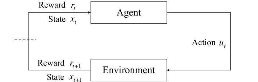
Figure 1: Markov decision process

Define $G_{t}=\sum_{i=t+1}^{T}\gamma^{i-t-1}r_{t}$ as the return, where $T$ is the terminal step. Our goal for the agent is to learn the optimal policy $\pi^{*}:x_{t}\rightarrow a_{t},\forall t\in\mathbb{Z^{+}}$, which satisfies

$$\pi^{*}=\max_{\pi\in\Pi}\mathbb{E}_{\pi}[G_{t}],\forall t\in\mathbb{Z^{+}},$$ (4)

where $\Pi$ is the set of all admissible policies. Detailed versions of $\mathbb{E}_{\pi}[G_{t}]$ are the state-value and the action-value

$$v_{\pi}(x_{t})=\mathbb{E}_{\pi}[G_{t}|x_{t}],$$ (5)

$$q_{\pi}(x_{t},a_{t})=\mathbb{E}_{\pi}[G_{t}|x_{t},a_{t}].$$

The Bellman equations reveal the recursion of $v_{\pi}(x_{t})$ and $q_{\pi}(x_{t},a_{t})$, which are given as follows:

$$v_{\pi}(x_{t})=\sum\limits_{x_{t+1}\in\mathbf{X}}\mathbf{P}_{x_{t}}^{x_{t+1}}\big{(}\pi(x_{t})\big{)}[\mathbf{R}_{x_{t}}^{x_{t+1}}\big{(}\pi(x_{t})\big{)}+\gamma v_{\pi}(x_{t+1})],$$ (6)

$$q_{\pi}(x_{t},a_{t})=\sum\limits_{x_{t+1}\in\mathbf{X}}\mathbf{P}_{x_{t}}^{x_{t+1}}(a_{t})[\mathbf{R}_{x_{t}}^{x_{t+1}}(a_{t})+\gamma q_{\pi}\big{(}x_{t+1},\pi(x_{t+1})\big{)}].$$

The optimal state-value and action-value are defined as

$$v^{*}(x_{t})=\max\limits_{\pi\in\Pi}v_{\pi}(x_{t}),\forall x_{t}\in\mathbf{X}$$ (7)

$$q^{*}(x_{t},a_{t})=\max\limits_{\pi\in\Pi}q_{\pi}(x_{t},a_{t}),\forall x_{t}\in\mathbf{X},\forall a_{t}\in\mathbf{A}.$$

For problems under the framework of the Markov decision process, $\pi^{*}$ can be obtained through many algorithms, e.g., policy iteration[21, 22]. Among them, we choose $Q$L due to its model-free, low computational complexity, and good scalability characteristics. In the following, we introduce $Q$L.

2.2.2 $Q$-Learning

$Q$L is a classical algorithm in reinforcement learning. The purpose of $Q$L is to enable the agent to find an optimal policy $\pi^{*}$ through interaction with the environment.

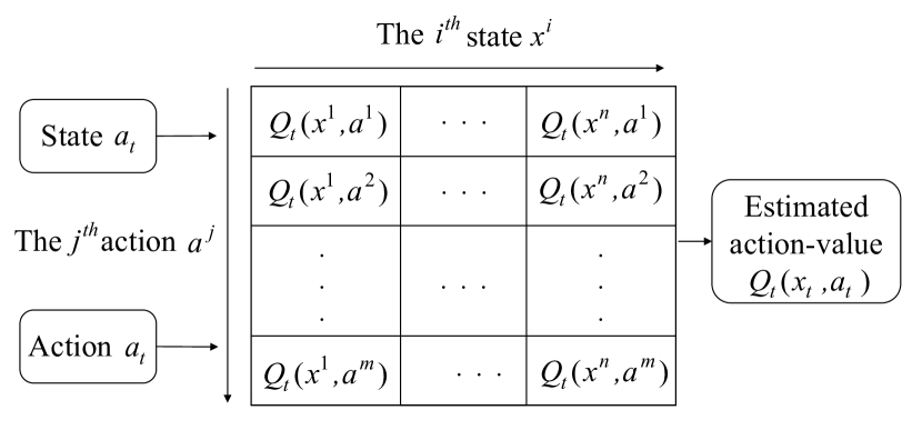
Figure 2: $Q$-table

As shown in Figure 2, $Q_{t}(x_{t},a_{t})$, namely, the estimate of $q^{*}(x_{t},a_{t})$ is recorded in the $Q$-table. The $Q$-table is updated every time step as follows:

$$Q_{t+1}(x,a)=\left\{\begin{aligned} &(1-\alpha_{t})Q_{t}(x,a)+\alpha_{t}TDE_{t},&&\text{if\ }(x,a)=\left(x_{t},a_{t}\right),\\ &Q_{t}(x,a),&&\text{else},\end{aligned}\right.$$ (8)

where $\alpha_{t}\in(0,1],t\in\mathbb{Z^{+}}$ is the learning rate, and $TDE_{t}$ is the temporal-difference error given as follows:

$$TDE_{t}=r_{t+1}+\gamma\max\limits_{u_{t+1}\in\mathbf{A}}Q_{t}(x_{t+1},a_{t+1})-Q_{t}(x_{t},a_{t}).$$ (9)

In terms of action selecting, $\epsilon$-greedy method is used

$$a_{t}=\left\{\begin{aligned} &\arg\max\limits_{a_{t}\in\mathbf{A}}Q_{t}\left(x_{t},a_{t}\right),&&P=1-\epsilon,\\ &\operatorname{rand}(\mathbf{A}),&&P=\epsilon,\\ \end{aligned}\right.$$ (10)

where $P$ is the probability to choose the action, $0\leq\epsilon\leq 1$, and $\operatorname{rand}(\mathbf{A})$ is an action randomly selected from $\mathbf{A}$.

$\mathbf{Lemma\ 1}$ [15]: $Q_{t}(x_{t},a_{t})$ converges to the fixed point $q^{*}(x_{t},a_{t})$ with probability one under the following conditions:

1. $\sum_{t=0}^{\infty}\alpha_{t}=\infty$ and $\sum_{t=0}^{\infty}\alpha_{t}^{2}<\infty$

2. $\operatorname{var}\left[r_{t}\right]$ is finite.

3. $|\mathbf{X}|$ and $|\mathbf{A}|$ are finite.

4. If $\gamma=1$, all policies lead to a cost-free terminal state with probability one.

Once $Q$L converges, the optimal policy $\pi^{*}$ is obtained as follows:

$$\pi^{*}\left(x_{t}\right)=\arg\underset{a_{t}\in\mathbf{A}}{\max}Q_{t}\left(x_{t},a_{t}\right),\forall x_{t}\in\mathbf{X}.$$ (11)

3 Finding Flip Kernels for Reachability

In this section, we first give the problem statement of finding flip kernels for reachability. Then, we propose three algorithms, namely, $Q$L, fast $Q$L, and small memory $Q$L for a large-scale system. Fast $Q$L improves the learning efficiency compared with $Q$L. Meanwhile, small memory $Q$L is applicable to large-scale systems.

Before presenting the specific problem of finding flip kernels for reachability, we give the definition of reachability.

$\mathbf{Definition\ 1}$: For a BCN with state flip control (3), assume that $\mathcal{M}_{0}\subset\mathcal{B}^{n}$ is the initial subset, and $\mathcal{M}_{d}\subset\mathcal{B}^{n}$ is the target subset. $\mathcal{M}_{d}$ is said to be reachable from $\mathcal{M}_{0}$ if and only if, for any initial state $x_{0}\in\mathcal{M}_{0}$, there exists a joint control pair sequence $\Big{\{}\big{(}u(t),\eta_{A(t)}\big{)},t=0,1,...,T\Big{\}}$, such that $x_{0}$ will reach a target state $x_{d}\in\mathcal{M}_{d}$.

$\mathbf{Problem\ 1}$: Based on Definition 1, we give the specific problem that we will consider. In some cases, it is not necessary to flip all nodes in $A$ for a BCN with state-flipped control (3) to realize reachability. To reduce the control cost, we hope the nodes that need to be flipped as fewer as possible. The above problem can be transformed into finding the flip kernels $B^{*}$ for reachability, which satisfies

$$\min_{B}|B|$$ (12)

s.t. $$B\subset A\text{\ and}$$

$$\mathcal{M}_{d}\text{\ is\ reachable\ from\ }\mathcal{M}_{0}\text{\ under\ the\ flip\ set\ }B.$$

It is worth noting that the flip kernels are not necessarily unique, since there may exist two or more flip sets with minimal cardinality such that the reachability is realized.

3.1 Markov Decision Process for Finding Flip Kernels

The premise for using $Q$L is structuring the problem into the framework of the Markov decision process. We represent the Markov decision process by the quintuple $(\mathcal{B}^{n},\mathcal{B}^{m+|B|},\mathbf{P},\mathbf{R},\gamma)$, where $\mathcal{B}^{n}$ and $\mathcal{B}^{m+|B|}$ are the state space and action space, respectively. The state and the action are defined as $x_{t}=x(t)$ and $a_{t}=\big{(}u(t),\eta_{A(t)}\big{)}$. The state-transition probability $\mathbf{P}$ is derived from the dynamics of BCNs with state-flipped control. Since the state transition is deterministic, $\mathbf{P}_{x_{t}}^{x_{t+1}}(a_{t})$ takes a value in {0,1}. For the same reason, the expected reward $\mathbf{R}_{x_{t}}^{x_{t+1}}(a_{t})$ which drives the agent to reach the target state can be simplified as $r_{t}$ given as follows:

$$r_{t}(x_{t},a_{t})=\left\{\begin{aligned} &100,&&x_{t}\in\mathcal{M}_{d},\\ &0,&&\text{else}.\\ \end{aligned}\right.$$ (13)

To encourage the agent reach $x_{t}\in\mathcal{M}_{d}$ as soon as possible, we set the discount factor $\gamma\in(0,1)$.

In terms of the prior system knowledge of the agent, it is assumed that the state dimension $n$ and the action dimension $m+|B|$ are known, while $\mathbf{P}$ and $\mathbf{R}$ aren't. The knowledge of $\mathbf{P}$ and $\mathbf{R}$ is learned gradually by the agent through its interaction with the environment. In the following, we give the algorithm, namely, $Q$L, for finding flip kernels.

3.2 Q-Learning for Finding Flip Kernels

Under the reward setting (13), we consider whether there exists a method to show the reachability. To answer the above question, we give Theorem 1.

$\mathbf{Theorem\ 1}$: It is assumed that $Q_{0}(x_{t},a_{t})=0,\forall x_{t},\forall a_{t}$ and (8) is used for updating $Q_{t}(x_{t},a_{t})$. The system (3) can realize reachability if and only if, there exists $t^{*}$ such that $\max_{a_{t}}Q_{t^{*}}(x_{0},a_{t})>0,\forall x_{0}\in\mathcal{M}_{0}$.

$\mathbf{Proof}$: (Necessity) Without loss of generality, it is assumed that there is only one $x_{0}\in\mathcal{M}_{0}$ and one $x_{d}\in\mathcal{M}_{d}$. Since the system (3) can realize reachability, for $x_{0}\in\mathcal{M}_{0}$, there exists a joint control pair sequence $\Big{\{}a_{t}=\big{(}u(t),\eta_{A(t)}\big{)},t=0,1,...,T\Big{\}}$, such that $x_{0}$ will reach the target state $x_{d}\in\mathcal{M}_{d}$. We apply $\Big{\{}a_{t}=\big{(}u(t),\eta_{A(t)}\big{)},t=0,1,...,T\Big{\}}$ to $x_{0}$, then we obtain a trajectory $x_{0}\stackrel{{\scriptstyle a_{0}}}{{\longrightarrow}}x_{1}\stackrel{{\scriptstyle a_{1}}}{{\longrightarrow}}...x_{T}\stackrel{{\scriptstyle a_{T}}}{{\longrightarrow}}x_{T+1}$, where $x_{T+1}\in\mathcal{M}_{d}$. Meanwhile, $x_{t}\stackrel{{\scriptstyle a_{t}}}{{\longrightarrow}}x_{t+1}$ means that $x_{t}$ will transform to $x_{t+1}$ when $a_{t}$ is taken.

As $Q$-learning runs, every state-action-state pair $(x_{t},a_{t},x_{t+1})$ are visited constantly[15]. Thus, there exists a case where $(x_{T},a_{T},x_{T+1})$, $(x_{T-1},a_{T-1},x_{T})$, $(x_{T-2},a_{T-2},x_{T-1})$, …,$(x_{0},a_{0},x_{1})$ are visited one after another, and between two adjacent ones, other state-action-state pairs can exist.

This causes values in the $Q$-table to go from being all zeros to some being zeros and others being positive. Specificly, the first update is $Q_{t^{\prime}}\big{(}x_{T},a_{T}\big{)}\leftarrow\alpha_{t^{\prime}}(r_{t^{\prime}+1}+\gamma\max\limits_{a_{t^{\prime}+1}}Q_{t^{\prime}-1}(x_{T+1},a_{t^{\prime}+1}))+(1-\alpha_{t^{\prime}})Q_{t^{\prime}-1}\big{(}x_{T},a_{T}\big{)}$. In the updated formula, we have $r_{t^{\prime}+1}=100$ since $x_{T+1}\in\mathcal{M}_{d}$. Meanwhile, notice that there is no negative reward as well as the initial action-values are all 0, so it follows that $Q_{t^{\prime}-1}(x_{T+1},a_{t^{\prime}+1})\geq 0,\forall t$. Thus, after the update, we have $Q_{t^{\prime}}\big{(}x_{T},a_{T}\big{)}>0$. Next, we prove that for $\forall t^{\prime\prime}>t^{\prime}$, it holds that $Q_{t^{\prime\prime}}\big{(}x_{T},a_{T}\big{)}>0$. For $\forall t$, notice that $r_{t}\geq 0$ as well as $Q_{t}(x_{t},a_{t})\geq 0,\forall(x_{t},a_{t})$. Thus, according to equation (8), for all $Q_{t}\big{(}x_{t},a_{t}\big{)}>0$, it holds that $Q_{t^{+}}\big{(}x_{t},a_{t}\big{)}>0,\forall t^{+}>t$. Consequently, we have $\forall t^{\prime\prime}>t^{\prime}$, it follows that $Q_{t^{\prime\prime}}\big{(}x_{T},a_{T}\big{)}>0$.

Next, based on mathematical induction, the proof that $Q_{t}\big{(}x_{t^{\prime}},a_{t^{\prime}}\big{)}>0,t^{\prime}=T-1,T-2,...,0$ is given. The proof is divided into two steps. First, we prove that if $(x_{t^{\prime}},a_{t^{\prime}},x_{t^{\prime}+1})$ is visited at time step $t$ and $Q_{t}\big{(}x_{t^{\prime}+1},a_{t^{\prime}+1}\big{)}>0$, then $Q_{t+1}\big{(}x_{t^{\prime}},a_{t^{\prime}}\big{)}>0$. Since $(x_{t^{\prime}},a_{t^{\prime}},x_{t^{\prime}+1})$ is visited at time step $t$, it follows that $Q_{t+1}\big{(}x_{t^{\prime}},a_{t^{\prime}}\big{)}\leftarrow\alpha_{t}(r_{t+1}+\gamma\max\limits_{a_{t}}Q_{t}(x_{t^{\prime}+1},a_{t}))+(1-\alpha_{t})Q_{t}\big{(}x_{t^{\prime}},a_{t^{\prime}}\big{)}$. In the updated formula, we have $r_{t+1}\geq 0$, and $Q_{t}\big{(}x_{t^{\prime}},a_{t^{\prime}}\big{)}\geq 0$. Meanwhile, since $Q_{t}\big{(}x_{t^{\prime}+1},a_{t^{\prime}+1}\big{)}>0$, it holds that $\max\limits_{a_{t}}Q_{t}(x_{t^{\prime}+1},a_{t})>0$. Consequently, we have $Q_{t}\big{(}x_{t^{\prime}+1},a_{t^{\prime}+1}\big{)}>0$. Sencond, we conclude that $Q_{t}\big{(}x_{t^{\prime}},a_{t^{\prime}}\big{)}>0,\ t^{\prime}=T-1$ because $Q_{t}\big{(}x_{T},a_{T}\big{)}>0$ . According to mathematics induction, there exists $t^{*}$ such that $Q_{t^{*}}\big{(}x_{0},a_{0}\big{)}>0$.

(Sufficiency) Without loss of generality, it is assumed that there is only one $x_{0}\in\mathcal{M}_{0}$ and one $x_{d}\in\mathcal{M}_{d}$. Suppose there exists $t^{*}$ such that $\max_{a_{t}}Q_{t^{*}}(x_{0},a_{t})>0$. Then, according to the updated formula $Q_{t^{*}}\big{(}x_{0},a_{t}\big{)}\leftarrow\alpha_{t^{*}-1}(r_{t^{*}}+\gamma\max\limits_{a_{t}}Q_{t^{*}-1}(x_{0\text{next}},a_{t}))+(1-\alpha_{t^{*}-1})Q_{t^{*}-1}\big{(}x_{0},a_{t}\big{)}$, where $x_{0\text{next}}$ is the subsequent state of $x_{0}$, at least one of the following two cases exists:

• Case 1. There exists $a_{t}$ and $x_{0\text{next}}$, such that $r_{t^{*}}(x_{0\text{next}},a_{t})>0$.

• Case 2. $x_{0\text{next}}$ satisfies $\max_{a_{t}}Q_{t^{*}-1}(x_{0\text{next}},a_{t})>0$.

For Case 1, we have $x_{0\text{next}}\in\mathcal{M}_{d}$, which means $\mathcal{M}_{d}$ is reachable from $x_{0}$ in one step.

In terms of Case 2, let us consider when will $\max_{a_{t}}Q_{t^{*}-1}(x_{0\text{next}},a_{t})>0$. First, we define the $i^{th}$ $Q$-value which change from 0 to a positive number as $Q_{ti}(x_{i},a_{i})$. Since the initial $Q$-values are all 0, it follows that $Q_{t1}(x_{1},a_{1})>0$ if and only if $x_{1\text{next}}\in\mathcal{M}_{d}$, which leads to $r_{t1}>0$. This indicates that $\mathcal{M}_{d}$ is reachable from $x_{1}$ in one step. Next, for any $i>1$, $Q_{ti}(x_{i},a_{i})>0$ appears if and only if $x_{i\text{next}}\in\mathcal{M}_{d}$, or $x_{i\text{next}}=x_{j},j<i$. This indicates at least one of the following two objects happen. Either $\mathcal{M}_{d}$ is reachable from $x_{i}$, or $x_{j},j<i$, a state can reach $\mathcal{M}_{d}$, is reachable from $x_{i}$. Both of them imply that $\mathcal{M}_{d}$ is reachable from $x_{i}$. Hence, if $\max_{a_{t}}Q_{t^{*}-1}(x_{0},a_{t})>0,\forall x_{0}\in\mathcal{M}_{0}$, then $\mathcal{M}_{d}$ is reachable from $\forall x_{0}\in\mathcal{M}_{0}$, which shows the reachability. $\hfill\blacksquare$

$\mathbf{Remark\ 1}$: The key for $Q$L to verify the reachability lies in the exploration(10) and the update rule of $Q$-table (8), instead of the convergence of $Q$L in Lemma 1.

$\mathbf{Lemma\ 2}$: We consider BCN with state-flipped control (3), $\mathcal{M}_{d}$ is reachable from $\forall x_{0}\in\mathcal{M}_{0}$ if and only if, there exists $l\leqslant 2^{n}-\left|\mathcal{M}_{d}\right|$ such that $\mathcal{M}_{d}$ is $l$-step reachable from $\forall x_{0}\in\mathcal{M}_{0}$.

$\mathbf{Proof}$: Without loss of generality, we assume there is a trajectory from $x_{0}\in\mathcal{M}_{0}$ to $\mathcal{M}_{d}$ whose length is greater than $2^{n}-\left|\mathcal{M}_{d}\right|$, then there must be at least one $x_{t}\in\mathcal{B}^{n}\setminus\mathcal{M}_{d}$ to be visited repeatedly. If we move the cycle from $x_{t}$ to $x_{t}$, the length of the trajectory will be less than $2^{n}-\left|\mathcal{M}_{d}\right|$.

$\hfill\blacksquare$

Based on Theorem 1 and Lemma 2, we give Algorithm 1 for finding flip kernels. The main idea of Algorithm 1 is that if the system can't realize reachability with flip sets with $|B|$ nodes, then we will increase the number of nodes to $|B|+1$ in the flip set, and check the reachability again. The process is repeated until reachability is achieved, and the criteria for achieving reachability is given by Theorem 1.

$\mathbf{Algorithm\ 1}$ Finding flip kernels for reachability of BCNs with state-flipped control using $Q$L

0:    $\mathcal{M}_{0}$, $\mathcal{M}_{d}$, $A$, $\alpha_{t}\in(0,1]$, $\gamma\in(0,1)$, $\epsilon\in[0,1]$, $N$, $T_{max}$

0:    Flip kernels

1:  $K=|A|$, $k=0$, $n=0$

2:  while  $k\leq K$  do

3:     for  $i=1,2,\dots,C_{|A|}^{k}$  do

4:        $B=B_{k_{i}}$

5:        Initialize $Q(x_{t},a_{t})\leftarrow 0,\forall x_{t}\in\mathcal{B}^{n},\forall a_{t}\in\mathcal{B}^{m+|B|}$

6:        for  $ep=0,1,\dots,N-1$  do

7:           $x_{0}\leftarrow\operatorname{rand}(\mathcal{M}_{0})$

8:           for $t=0,1,\dots,T_{max}-1$ and $x_{t}\notin\mathcal{M}_{d}$ do

9:              $a_{t}\leftarrow\left\{\begin{aligned} &\arg\max_{a_{t}}Q(x_{t},a_{t}),&&P=1-\epsilon\\ &\operatorname{rand}(\mathcal{B}^{m+|B|}),&&P=\epsilon\end{aligned}\right.$

10:              $Q(x_{t},a_{t})\leftarrow\alpha_{t}(r_{t+1}+\gamma\max\limits_{a_{t+1}}Q(x_{t+1},a_{t+1}))+(1-\alpha_{t})Q(x_{t},a_{t})$

11:           end for

12:           if $\max_{a_{t}}Q(x_{t},a_{t})>0,\forall x_{t}\in\mathcal{M}_{0}$ then

13:              $B_{n}^{*}=B$, $K=|B|$, $n=n+1$

14:              Break

15:           end if

16:        end for

17:     end for

18:     $k=k+1$

19:  end while

20:  if $n=0$ then

21:     return  ``The system can't realize reachability."

22:  else

23:     return  $B^{*}_{1},\dots,B^{*}_{n}$

24:  end if

Next, we give the definition of notations in Algorithm 1. $C_{|A|}^{k}$ is the combinatorial number of flip sets with $k$ nodes in $A$. $B_{k_{i}}$ is the $i^{th}$ flip set with $k$ nodes. $ep$ means the number of episodes. ``Episode" is a reinforcement learning term. An episode means a period of interaction that has passed through $T_{max}$ time steps from any initial state $x_{0}$. The introduction of $ep$ helps the agent visit every $x_{0}\in\mathcal{M}_{0}$, so as to check reachability. $T_{max}$ is the maximum time step, which should be greater than the length of the trajectory from $\mathcal{M}_{0}$ to $\mathcal{M}_{d}$. Otherwise, even if the system is reachable, the agent may not get positive feedback $r_{t}>0$ in $T_{max}$ steps, which invalidates the algorithm. The setting of $T_{max}$ can refer to Lemma 2.

$\mathbf{Remark\ 2}$: When the system is reachable, if we delete steps 12-15, then we will obtain the policy under which the steps are minimal to realize reachability. It is because the agent receives $r_{t}>0$ only when it reaches $\mathcal{M}_{d}$, and since $\gamma<1$, the return $\sum_{i=t+1}^{T}\gamma^{i-t-1}r_{t}$ is the highest when the reachability is realized with minimal steps.

Algorithm 1 still has room for improvement. Next, we add some tricks to Algorithm 1, which will improve efficiency.

3.3 Fast Q-learning for Finding Flip Kernels

In this subsection, we propose Algorithm 2, namely, fast $Q$-learning for finding flip kernels, which improves learning efficiency. The main difference between Algorithm 2 and Algorithm 1 can be divided into two aspects. 1) Special initial states: Algorithm 2 chooses initial states strategically instead of randomly. 2) TL: Algorithm 2 collects experience for the reachability of the system with the smaller flip sets tested before, and applies it to find flip kernels of the system with larger flip sets.

$\mathbf{Algorithm\ 2}$ Finding flip kernels for reachability of BCNs with state-flipped control using fast $Q$L

0:    $\mathcal{M}_{0}$, $\mathcal{M}_{d}$, $A$, $\alpha_{t}\in(0,1]$, $\gamma\in(0,1)$, $\epsilon\in[0,1]$, $N$, $T_{max}$

0:    Flip kernels

1:  $K=|A|$, $k=0$, $n=0$

2:  while  $k\leq K$  do

3:     for  $i=1,2,\dots,C_{|A|}^{k}$  do

4:        $B=B_{k_{i}}$

5:        Initialize $Q(x_{t},a_{t}),\forall x_{t}\in\mathcal{B}^{n},\forall a_{t}\in\mathcal{B}^{m+|B|}$ using (14)

6:        for  $ep=0,1,\dots,N-1$  do

7:           $x_{0}\leftarrow\operatorname{rand}\big{(}\{x_{0}\in\mathcal{M}_{0}|\max_{a_{t}}Q(x_{t},a_{t})=0\}\big{)}$

8:           for $t=0,1,\dots,T_{max}-1$ and $x_{t}\notin\mathcal{M}_{d}$ do

9:              $a_{t}\leftarrow\left\{\begin{aligned} &\arg\max_{a_{t}}Q(x_{t},a_{t}),&&P=1-\epsilon\\ &\operatorname{rand}(\mathcal{B}^{m+|B|}),&&P=\epsilon\end{aligned}\right.$

10:              $Q(x_{t},a_{t})\leftarrow\alpha_{t}(r_{t+1}+\gamma\max\limits_{a_{t+1}}Q(x_{t+1},a_{t+1}))+(1-\alpha_{t})Q(x_{t},a_{t})$

11:           end for

12:           if $\max_{a_{t}}Q(x_{t},a_{t})>0,\forall x_{t}\in\mathcal{M}_{0}$ then

13:              $B_{n}^{*}=B$, $K=|B|$, $n=n+1$

14:              Break

15:           end if

16:        end for

17:        Record the $Q$-table for $B$

18:     end for

19:     Drop all the $Q$-tables, $k=k+1$

20:  end while

21:  if $n=0$ then

22:     return  ``The system can't realize reachability."

23:  else

24:     return  $B^{*}_{1},\dots,B^{*}_{n}$

25:  end if

3.3.1 Special Initial States

The main idea of special initial states is that we do not need to visit $x_{0}\in\mathcal{M}_{0}$, once we know $\mathcal{M}_{d}$ is reachable from $x_{0}$. Instead, we focus on states in $\mathcal{M}_{0}$ that are not found to be reachable. Based on the idea, we change step 7 in Algorithm 1 to that in Algorithm 2.

$\mathbf{Remark\ 3}$: Theorem 1 still holds when we add special initial states into $Q$-learning, since the trajectory from states in $\mathcal{M}_{0}$ that are not found to be reachable to $\mathcal{M}_{d}$ can still be visited.

3.3.2 Transfer-learning

Consider the relationship between $Q^{B}(x_{t},a_{t})$ and $Q^{b}(x_{t},a_{t})$, namely, the $Q$-table with the flip set $B$ and those with the flip sets $b\subset B$. Theorem 2 is proposed to explain it.

$\mathbf{Theorem\ 2}$: For any state-action pairs $(x_{t},a_{t})$, if $Q^{b}(x_{t},a_{t})>0$ with a flip set $b\subset B$, then $Q^{B}(x_{t},a_{t})>0$ holds for flip set $B$.

$\mathbf{Proof}$: It is easy to see that the action space according to the flip sets $b\subset B$ is the subset of the action space of the flip set $B$, namely, $\mathbf{A}_{b}\subset\mathbf{A}_{B}$. Thus, if $x_{1}$ is reachable to $x_{d}\in\mathcal{M}_{d}$ with the flip sets $b\subset B$, namely, there exists a tragetory $x_{1}\stackrel{{\scriptstyle a_{1}}}{{\longrightarrow}}x_{2}...\stackrel{{\scriptstyle a_{T}}}{{\longrightarrow}}x_{d},\ a_{t}\in\mathbf{A}_{b}$, the reachability still holds with the flip set $B$ since the tragetory $x_{1}\stackrel{{\scriptstyle a_{1}}}{{\longrightarrow}}x_{2}...\stackrel{{\scriptstyle a_{T}}}{{\longrightarrow}}x_{d},\ a_{t}\in\mathbf{A}_{b}\subset\mathbf{A}_{B}$ exists. This indicates that if $x_{1}$ is reachable to $x_{d}\in\mathcal{M}_{d}$ with the flip sets $b\subset B$, then the reachability holds with the flip set $B$.

From Theorem 1, $x_{1}$ can reach $x_{d}\in\mathcal{M}_{d}$ when the first control input in the sequence is $a_{1}$ if and only if $Q(x_{1},a_{1})>0$. Hence, for any state-action pairs $(x_{t},a_{t})$, if $Q^{b}(x_{t},a_{t})>0$ with flip set $b\subset B$, then $Q^{B}(x_{t},a_{t})>0$ holds for flip set $B$. $\hfill\blacksquare$

Motivated by the above results, we consider TL [23]. TL improves the process of learning in a new task through the transfer of knowledge from a related task that has already been learned. Here, we utilize TL by initializing the $Q$-table for the flip set $B$ with the knowledge of that for the flip sets $b\subset B$, namely

$$Q_{0}(x_{t},a_{t})=\left\{\begin{aligned} &0,&&\text{\ not\ exist\ }b\subset B,\text{s.t.}a_{t}\in b,\\ &\max_{b\subset B}Q_{t}^{b}(x_{t},a_{t}),&&\text{else},\end{aligned}\right.$$ (14)

where $Q_{t}^{b}(x_{t},a_{t})$ is the $Q$-table according to the flip set $b$. Based on the idea, step 5 in Algorithm 1 is changed in Algorithm 2, and steps 17 and 19 are added.

Algorithm 2 increases the learning efficiency compared with Algorithm 1. However, there is still an improvement for Algorithm 2. Specifically, the operation of $Q$L is based on a $Q$-table with $|\mathbf{X}|\times|\mathbf{A}|$ values, the number of which is $2^{n+m+|B|}$. Notice that the number grows exponentially with $n$ and $m+|B|$. When $n$ and $m+|B|$ are too large, $Q$-learning is no longer applicable, since the $Q$-table is too large to store in the computer. Inspired by [24], we propose an algorithm for large-scale systems in the following subsection, generally speaking, systems with more than 20 nodes.

3.4 Small Memory Q-Learning for Finding Flip Kernels of Large-scale BCNs

In this subsection, we proposed Algorithm 3, namely, small memory $Q$L, to find flip kernels for large-scale systems. Another model-free method to deal with the control problem of large-scale BCNs is D$Q$N[25], which is a deep reinforcement method. However, it not only has no guarantee of convergence, but also has high computational complexity. For these reasons, we proposed Algorithm 3, which is inspired by [24]. The main idea of Algorithm 3 is that we only record action-values for states which have been visited, instead of all $x_{t}\in\mathcal{B}^{n}$, so as to reduce the memory. Based on the idea, step 5 in Algorithm 1 is changed in Algorithm 3, and steps 10-12 are added. Next, we give the specific effect and the applicable systems of Algorithm 3.

$\mathbf{Algorithm\ 3}$ Finding flip kernels for reachability of BCNs with state-flipped control using small memory $Q$L

0:    $\mathcal{M}_{0}$, $\mathcal{M}_{d}$, $A$, $\alpha_{t}\in(0,1]$, $\gamma\in(0,1)$, $\epsilon\in[0,1]$, $N$, $T_{max}$

0:    Flip kernels

1:  $K=|A|$, $k=0$, $n=0$

2:  while  $k\leq K$  do

3:     for  $i=1,2,\dots,C_{|A|}^{k}$  do

4:        $B=B_{k_{i}}$

5:        Initialize $Q(x_{t},a_{t})\leftarrow 0,\forall x_{t}\in\mathcal{M}_{0},\forall a_{t}\in\mathcal{B}^{m+|B|}$

6:        for  $ep=0,1,\dots,N-1$  do

7:           $x_{0}\leftarrow\operatorname{rand}(\mathcal{M}_{0})$

8:           for $t=0,1,\dots,T_{max}-1$ and $x_{t}\notin\mathcal{M}_{d}$ do

9:              $a_{t}\leftarrow\left\{\begin{aligned} &\arg\max_{a_{t}}Q(x_{t},a_{t}),&&P=1-\epsilon\\ &\operatorname{rand}(\mathcal{B}^{m+|B|}),&&P=\epsilon\end{aligned}\right.$

10:              if $Q(x_{t+1},.)$ is not in the $Q$-table then

11:                 Add $Q(x_{t+1},.)=0$ to the $Q$-table

12:              end if

13:              $Q(x_{t},a_{t})\leftarrow\alpha_{t}(r_{t+1}+\gamma\max\limits_{a_{t+1}}Q(x_{t+1},a_{t+1}))+(1-\alpha_{t})Q(x_{t},a_{t})$

14:           end for

15:           if $\max_{a_{t}}Q(x_{t},a_{t})>0,\forall x_{t}\in\mathcal{M}_{0}$ then

16:              $B_{n}^{*}=B$, $K=|B|$, $n=n+1$

17:              Break

18:           end if

19:        end for

20:     end for

21:     $k=k+1$

22:  end while

23:  if $n=0$ then

24:     return  ``The system can't realize reachability."

25:  else

26:     return  $B^{*}_{1},\dots,B^{*}_{n}$

27:  end if

Based on Algorithm 3, the action-value needs to be recorded is reduced from $2^{n+m+|B|}$ to $|V+\mathcal{M}_{0}|\times 2^{m+|B|}$, where $V=\{x_{t}|\ x_{t}$ is reachable from $x_{0},\ \forall x_{0}\in\mathcal{M}_{0}\}$. The estimation of $|V|$ can be referred to Lemma 3. Before presenting Lemma 3, we first introduce Definition 2.

$\mathbf{Definition\ 2}$: The in-degree of $x_{t}$ is defined as the number of states which can reach $x_{t}$ in one step with $\overline{a_{t}}=\big{(}u(t),\eta_{A}(t)\big{)}$ where $|\eta_{A(t)}|_{\infty}=0$, namely, an action without state-flipping.

$\mathbf{Lemma\ 3}$: Assume that the in-degree of $x_{t+1}$ is more than 0, it holds that $|V|\leq|I|$, where $I=\{x_{t}|\$the in-degree of $x_{t}$ is more than 0 $\}$.

$\mathbf{Proof}$: First, consider the normal case where $V$ is generated, namely, BCNs with state-flipped control. The process of state transition can be divided into two steps. For any $x_{t}\in\mathcal{B}^{n}$, according to $\eta_{A(t)}$, it first be flipped into $\eta_{A(t)}(x_{t})\in\mathcal{B}^{n}$. Then, based on $u(t)$, namely, $\overline{a_{t}}$, $\eta_{A(t)}(x_{t})$ tranfers to $x_{t+1}$. Notice that $x_{t+1}\in I$ holds. Thus, $x_{t}$ can only reach $x_{t+1}\in I$ even with state-flipped control. Meanwhile, $x_{t}$ can reach $\forall x_{t+1}\in I$ according to the definition of $I$. Consequetly, we have $I=\{x_{t+1}|\ \exists x_{t}\in\mathcal{B}^{n}$, such that $x_{t+1}$ is reachable from $x_{t}\}$. Notice that $\mathcal{M}_{0}\subset\mathcal{B}^{n}$. Hence, $V=\{x_{t+1}|\ \exists x_{t}\in\mathcal{M}_{0}$, such that $\ x_{t+1}$ is reachable from $x_{0}\}\subset I$. Then, it can be concluded that $|V|\leq|I|$. $\hfill\blacksquare$

Algorithm 3 can reduce the number stored in the $Q$-table from $2^{n+m+|B|}$ to $|V+\mathcal{M}_{0}|\times 2^{m+|B|}$. However, we acknowledge that when $|V+\mathcal{M}_{0}|\times 2^{m+|B|}$ is too large, $Q$L has some limitations. Importantly, Algorithm 3 provides a possibility to solve problems for large-scale systems, instead of the traditional $Q$L which simply be regarded as inapplicable.

$\mathbf{Remark\ 4}$: The idea of special initial states and TL in Algorithm 2 can also be added to Algorithm 3. The hybrid algorithm obtained not only improves the efficiency of learning, but can also be applied to large-scale systems.

4 Minimum Flipping Actions for Reachability Using Q-Learning

In this section, we first give the problem statement, namely, finding the optimal policy under which the reachability can be realized using minimum flipping actions. Then, we present the reward setting under which the highest return is obtained only if the corresponding policy meets the goal. At last, two algorithms for obtaining the optimal policies are given, namely, $Q$L, and small memory $Q$L for large-scale systems.

$\mathbf{Problem\ 2}$: To reduce control costs, we hope to find the optimal policy, under which the reachability can be realized using minimum flipping actions. The above problem can be transformed into finding the policy $\pi^{*}$ for the reachability, which satisfies

$$\min_{\pi}\sum_{t=0}^{T}n_{t}$$ (15)

s.t. $$\mathcal{M}_{d}\text{\ is\ reachable\ from\ }\mathcal{M}_{0},$$

where $n_{t}$ is the number of the nodes to be flipped at $t$, $T$ is the terminal time step. The terminal states are defined as $\forall x_{d}\in\mathcal{M}_{d}$. It is worth noting that $\pi^{*}$ is not necessarily unique, since there may exist two or more $\pi^{*}$ such that the reachability is realized with minimum flipping actions.

4.1 Markov Decision Process for Finding Minimum Flipping Actions

Since $Q$L will be used to find $\pi^{*}$, we first construct the problem into the framework of the Markov decision process. Let the Markov decision process be the quintuple $(\mathcal{B}^{n},\mathcal{B}^{m+|B^{*}|},\gamma,\mathbf{P},\mathbf{R})$. To drive the agent to realize reachability with minimal flipping actions, we define $r_{t+1}$ as follows:

$$r_{t}(x_{t},a_{t})=\left\{\begin{aligned} &-w\times n_{t},&&x_{t}\in\mathcal{M}_{d},\\ &-w\times n_{t}-1,&&\text{else},\\ \end{aligned}\right.$$ (16)

where $w>0$ is the weight. $r_{t}$ can be divided into two parts. One is ``-1'', which is obtained when the agent hasn't reached $\mathcal{M}_{d}$. To avoid negative feedback ``-1'', the agent will realize reachability as soon as possible. The other is ``$-w\times n_{t}$'', which drives the agent to use as less flipping actions as possible.

$\mathbf{Remark\ 5}$: The following analysis is based on the assumption that the system can realize reachability. Whether the assumption is satisfied can be tested through Theorem 1.

The value of $w$ is the key to accurately conveying the goal (15) to the agent. If $w$ is too small, the goal of realizing reachability as soon as possible will submerge the goal of taking minimum flipping actions. To illustrate the problem more vividly, let's take an example.

$\mathbf{Example\ 1}$: Without loss of generality, it is assumed that there is only one $x_{0}\in\mathcal{M}_{0}$ and one $x_{d}\in\mathcal{M}_{d}$. Supposed there exist two policies $\pi_{1}$ and $\pi_{2}$. When we start with $x_{0}$ and take $\pi_{1}$, we get the trajectory $x_{0}\rightarrow x_{1}\rightarrow x_{2}\rightarrow x_{3}\rightarrow x_{d}$ without flipping action. And if we take $\pi_{2}$, then the trajectory $x_{0}\rightarrow x_{d}$ with 2 flipping actions will be obtained. It can be calculated that $v_{\pi_{1}}(x_{0})=-4$ since the agent takes 4 steps to realize reachability without flipping actions. Meanwhile, $v_{\pi_{1}}(x_{0})=-1-2w$ since the agent takes 1 step to realize reachability with 2 flipping actions. In this case, if we set $w=1$, then it will follow that $v_{\pi_{1}}(x_{0})<v_{\pi_{2}}(x_{0})$, which means that the return after adopting $\pi_{2}$ is higher. In other words, utilizing the policy which requires more flipping actions to realize reachability will lead to higher return. Obviously, this does not help us find $\pi^{*}$ to achieve the goal (15).

So, how big $w$ should be such that the goal (15) can be achieved? To answer the question, Theorem 3 and Corollary 1, the sufficient conditions that ensure the optimality of policy, are proposed. The core idea of design $w$ is to make $v_{\pi^{*}}(x_{0})>v_{\pi}(x_{0}),\forall\pi\in\Pi,$ and $\pi\neq\pi^{*}$, where $\pi^{*}$ satisfies the goal (15).

$\mathbf{Theorem\ 3}$: For a BCN with state-flipped control (3), if $w>l$, where $l$ is the largest length for any $x_{0}\in\mathcal{M}_{0}$ to reach $\mathcal{M}_{d}$ without cycles, then the optimal policy obtained according to (16) satisfies the goal (15).

$\mathbf{Proof}$: Without loss of generality, it is assumed that there is only one $x_{0}\in\mathcal{M}_{0}$. Next, we classify all $\pi\in\Pi$ and prove that the one with the highest state-value satisfies the goal (15), under the condition that $w>l$. For all $\pi\in\Pi$, we can divide them into 2 cases:

• Case 1. Following $\pi_{1}$, $\mathcal{M}_{d}$ can not be reached.

• Case 2. Following $\pi_{2}$, $\mathcal{M}_{d}$ can be reached from $x_{0}$.

For Case 1, $v_{\pi_{1}}(x_{0})=\sum_{t=0}^{-\infty}-1=-\infty$. $v_{\pi_{1}}(x_{0})$ is too small to let $\pi_{1}$ be the optimal one. For Case 2, we divide it into two subcases:

• Case 2.1. Following $\pi_{2.1}$, $\mathcal{M}_{d}$ is reached from $x_{0}$ with less flipping actions.

• Case 2.2. Following $\pi_{2.2}$, $\mathcal{M}_{d}$ is reached from $x_{0}$ with more flipping actions.

Next, we compare the magnitude of $v_{\pi_{2.1}}$ and $v_{\pi_{2.2}}$. Assume that it takes $T_{\pi_{2.1}}$ steps with $\sum n_{\pi_{2.1}}$ flipping actions, and $T_{\pi_{2.2}}$ steps with $\sum n_{\pi_{2.2}}$ flipping actions for $x_{0}$ to reach $\mathcal{M}_{d}$ under $\pi_{2.1}$ and $\pi_{2.2}$, respectively. Then, we can obtain $v_{\pi_{2.1}}=-w\sum n_{\pi_{2.1}}-T_{\pi_{2.1}}$ and $v_{\pi_{2.2}}=-w\sum n_{\pi_{2.2}}-T_{\pi_{2.2}}$. It is calculated that $v_{\pi_{2.1}}-v_{\pi_{2.2}}=w\sum n_{\pi_{2.2}}+T_{\pi_{2.2}}-w\sum n_{\pi_{2.1}}-T_{\pi_{2.1}}$. Since more flipping actions are taken under $\pi_{2.2}$ than $\pi_{2.1}$ to realize reachability, then one has $\sum n_{\pi_{2.2}}-\sum n_{\pi_{2.1}}>0$.

In terms of relationship between $T_{\pi_{2.1}}$ and $T_{\pi_{2.2}}$, there are two categories:

• Category 1. $T_{\pi_{2.1}}\leq T_{\pi_{2.2}}$.

• Category 2. $T_{\pi_{2.1}}>T_{\pi_{2.2}}$.

For Category 1, it's obvious that $v_{\pi_{2.1}}>v_{\pi_{2.2}}$. For Category 2, we divide $\pi_{2.1}$ into two cases.

• Case 2.1.1. Following $\pi_{2.1.1}$, $x_{0}$ can reach $\mathcal{M}_{d}$ in $T_{\pi_{2.1.1}}\leq l$ steps with $\sum n_{\pi_{2.1.1}}<\sum n_{\pi_{2.2}}$ flipping actions, where $l$ is the maximum length of the trajectory from $x_{0}$ to $\mathcal{M}_{d}$ without cycle.

• Case 2.1.2. Following $\pi_{2.1.2}$, $x_{0}$ can reach $\mathcal{M}_{d}$ in $T_{\pi_{2.1.2}}>l$ steps with $\sum n_{\pi_{2.1.2}}<\sum n_{\pi_{2.2}}$ flipping actions.

Next, the proof that $v_{\pi_{2.1.1}}>v_{\pi_{2.2}}$ is given. For Case 2.1.1, we have the following inequality

$$\left\{\begin{aligned} &T_{\pi_{2.2}}-T_{\pi_{2.1.1}}\geq T_{min}-l\geq 1-l,\\ &\sum n_{\pi_{2.2}}-\sum n_{\pi_{2.1.1}}\geq 1,\\ \end{aligned}\right.$$ (17)

where $T_{min}$ is the minumum length of the trajectory from $x_{0}$ to $\mathcal{M}_{d}$. Substitute (17) into $v_{\pi_{2.1.1}}-v_{\pi_{2.2}}=T_{\pi_{2.2}}-T_{\pi_{2.1.1}}+w(\sum n_{\pi_{2.2}}-\sum n_{\pi_{2.1.1}})$, we have $v_{\pi_{2.1.1}}-v_{\pi_{2.2}}\geq 1-l+w$. Since $w>l$, it follows that $v_{\pi_{2.1.1}}-v_{\pi_{2.2}}>0$.

In the following, we discuss Case 2.1.2. Notice that $T_{\pi_{2.1.2}}>l$, according to Lemma 2, at least one $x_{t}\in\mathcal{B}^{n}\backslash\mathcal{M}_{d}$ is visited repeatedly. If we remove the cycle from the trajectory, then its length will be no greater than $l$, and its flipping actions are fewer. This indicates the existence of $\pi_{2.1.2}^{*}$, which satisfies $T_{\pi_{2.1.2}^{*}}\leq l$. and $\sum n_{\pi_{2.1.2}^{*}}\leq\sum n_{\pi_{2.1.2}}<\sum n_{\pi_{2.2}}$. Thus, $\pi_{2.1.2}^{*}$ is consistent with Case 2.1.1. Based on the proof in the previous paragraph, we have $v_{\pi_{2.1.2}^{*}}(x_{0})>v_{\pi_{2.2}}(x_{0})$. Also, it is easy to find $v_{\pi_{2.1.2}^{*}}(x_{0})>v_{\pi_{2.1.2}}(x_{0})$. Therefore, it can be concluded that $\pi_{2.1.2}^{*}$ is the one with the highest return compared with $\pi_{2.2}$ and $\pi_{2.1.2}$.

After analyzing various cases, we conclude that when $w>l$, $\pi$ with the highest $v_{\pi}(x_{0})$ satisfies the goal (15). $\hfill\blacksquare$

$\mathbf{Corollary\ 1}$: For the case where there is no prior knowledge, if $w>2^{n}-|\mathcal{M}_{d}|$, then the optimal policy obtained according to (16) satisfies the goal (15).

$\mathbf{Proof}$: The upper bound of $l$ in Theorem 3 can be given through Lemma 2, which is $l\leq 2^{n}-|\mathcal{M}_{d}|$. Thus, we will easily get $w>l$, which is the sufficient condition ensuring the optimality of policy, as long as $w>2^{n}-|\mathcal{M}_{d}|$. $\hfill\blacksquare$

$\mathbf{Remark\ 6}$: For Theorem 3 and Corollary 1, two objects should be clarified. First, following Theorem 3 or Corollary 1, we do not get all $\pi^{*}$ that satisfy the goal (15), but $\pi^{*}$ that satisfies the goal (15) with the shortest time to realize reachability. Second, Theorem 3 and Corollary 1 are sufficient but not necessary conditions for the optimality of the obtained policy, in that (17) uses the inequality scaling technique.

Now, we have the reward (16) under which $\pi^{*}$ with the highest $v_{\pi}(x_{0})$ satisfies the goal (15). Next, we present $Q$L for finding $\pi^{*}$.

4.2 Q-Learning for Finding Minimum Flipping Actions

In this subsection, we propose $Q$L for finding minimum flipping actions for the reachability of BCNs with state-flipped control.

$\mathbf{Algorithm\ 4}$ Finding minimum flipping actions for reachability of BCNs with state-flipped control using $Q$L

0:    $\mathcal{M}_{0}$, $\mathcal{M}_{d}$, $B^{*}$, $\alpha_{t}\in(0,1]$, $\gamma=1$, $\epsilon\in[0,1)$, $N$, $T_{max}$

0:    $\pi^{*}$

1:  Initialize $Q(x_{t},a_{t})\leftarrow 0,\forall x_{t}\in\mathcal{B}^{n},\forall a_{t}\in\mathcal{B}^{m+|B^{*}|}$

2:  for  $ep=0,1,\dots,N-1$  do

3:     $x_{0}\leftarrow\operatorname{rand}(\mathcal{M}_{0})$

4:     for $t=0,1,\dots,T_{max}-1$ and $x_{t}\notin\mathcal{M}_{d}$ do

5:        $a_{t}\leftarrow\left\{\begin{aligned} &\arg\max_{a_{t}}Q(x_{t},a_{t}),&&P=1-\epsilon\\ &\operatorname{rand}(\mathcal{B}^{m+|B|}),&&P=\epsilon\end{aligned}\right.$

6:        $Q(x_{t},a_{t})\leftarrow\alpha_{t}(r_{t+1}+\gamma\max\limits_{a_{t+1}}Q(x_{t+1},a_{t+1}))+(1-\alpha_{t})Q(x_{t},a_{t})$

7:     end for

8:  end for

9:  return  $\pi^{*}(x_{t})\leftarrow\arg\max\limits_{a_{t}\in\mathbf{A}}Q(x_{t},a_{t}),\forall x_{t}\in\mathbf{X}$

Next, the parameter requirements are given. In terms of $T_{max}$, it should be larger than the maximum length of trajectory from $x_{0}$ to $\mathcal{M}_{d}$ without cycle, which is given by Lemma 2. Otherwise, the agent may be unable to reach the terminal $\mathcal{M}_{d}$ before the end of the episode, which violates condition 4) of Lemma 1. In terms of $\epsilon$, it should satisfy $\epsilon<1$, which guarantees the exploration of the agent. Hence, the policies during learning are not deterministic, namely, all the policies can adopt reachable control sequences with a certain probability, which satisfies condition 4) of Lemma 1.

Algorithm 4 can find $\pi^{*}$ for small-scale BCNs with state-flipped control. However, when $n$ and $m+|B|$ are too large, Algorithm 4 is no longer applicable since the $Q$-table is too large to store in the computer. This motivates us to utilize small memory $Q$-learning in Section IIID.

4.3 Fast Small Memory Q-Learning for for Finding Minimum Flipping Actions of Large-scale Systems

In this section, we propose Algorithm 5, namely, fast small memory $Q$L for finding minimum flipping actions for reachability of large-scale BCNs with state-flipped control. Two changes are made from Algorithm 4 to 5.

$\mathbf{Algorithm\ 5}$ Finding minimum flipping actions for reachability of large-scale BCNs with state-flipped control using small memory $Q$L

0:    $\mathcal{M}_{0}$, $\mathcal{M}_{d}$, $B^{*}$, $\alpha_{t}\in(0,1]$, $\gamma=1$, $\epsilon\in[0,1)$, $N$, $T_{max}$, $w$, $\Delta w>0$

0:    $\pi^{*}$

1:  Initialize $Q(x_{t},a_{t})\leftarrow 0,\forall x_{t}\in\mathcal{M}_{0},\forall a_{t}\in\mathcal{B}^{m+|B^{*}|}$

2:  for  $ep=0,1,\dots,N-1$  do

3:     $x_{0}\leftarrow\operatorname{rand}(\mathcal{M}_{0})$

4:     if $w\leq\big{|}\{x_{t}|\ Q(x_{t},.)$ is in the $Q$-table$\}\big{|}$ then

5:        $w=w+\Delta w$

6:     end if

7:     for $t=0,1,\dots,T_{max}-1$ and $x_{t}\notin\mathcal{M}_{d}$ do

8:        $a_{t}\leftarrow\left\{\begin{aligned} &\arg\max_{a_{t}}Q(x_{t},a_{t}),&&P=1-\epsilon\\ &\operatorname{rand}(\mathcal{B}^{m+|B|}),&&P=\epsilon\end{aligned}\right.$

9:        if $Q(x_{t+1},.)$ is not in the $Q$-table then

10:           Add $Q(x_{t+1},.)=0$ to the $Q$-table

11:        end if

12:        $Q(x_{t},a_{t})\leftarrow\alpha_{t}(r_{t+1}+\gamma\max\limits_{a_{t+1}}Q(x_{t+1},a_{t+1}))+(1-\alpha_{t})Q(x_{t},a_{t})$

13:     end for

14:  end for

15:  return  $\pi^{*}(x_{t})\leftarrow\arg\max\limits_{a_{t}\in\mathbf{A}}Q(x_{t},a_{t}),\forall x_{t}\in\mathbf{X}$

First, only the action-values of the states that have been visited are recorded, which reflects in steps 1, and 9-11 in Algorithm 5. The idea and the effect of Algorithm 5 are the same as that in Algorithm 3.

Second, $w$ which influences $r_{t}$ is no longer a constant, but a variable changing according to $Q=\big{|}\{x_{t}|\ Q(x_{t},.)$ is in the $Q$-table$\}\big{|}$, which reflects in steps 4-6. With the exploration of the agent, $\big{|}Q\big{|}$ increases and finally equals to $|V+\mathcal{M}_{0}|$. Here, we do not simply set $w=2^{n}+1-|\mathcal{M}_{d}|$ according to Corollary 1, in that for large-scale systems, $2^{n}+1-|\mathcal{M}_{d}|$ is so big that the weight for using less flipping actions will be far more than realizing reachability as soon as possible. This will confuse the agent. At the beginning of the learning process, the agent always gets large negative feedback when it takes flipping actions, but less negative feedback when it doesn’t realize reachability. As long as the small negative feedback for not realizing reachability accumulated enough than the large negative feedback for flipping actions, will the agent realize it is worth taking flipping actions to achieve reachability. The larger the $w$, the longer the process will be. Thus, we consider the scaling for $w$ to speed up the process. The main idea of scaling is using the knowledge learned by the agent while satisfying the condition in Theorem 3 to guarantee the optimality of the policy. Next, we give Theorem 4 to explain it.

$\mathbf{Theorem\ 4}$: For a BCN with state-flipped control (3), if it holds that $w>|Q|$, then the optimal policy obtained according to (16) satisfies the goal (15).

$\mathbf{Proof}$: First, we prove that $\mathcal{M}_{d}$ is reachable from $\forall x_{0}\in\mathcal{M}_{0}$ if and only if, there exists $l\leq|V|$ such that $\mathcal{M}_{d}$ is $l$-step reachable from $\forall x_{0}\in\mathcal{M}_{0}$. $\mathcal{M}_{d}$ is said to be reachable from $\mathcal{M}_{0}$ if and only if, for any initial state $x_{0}\in\mathcal{M}_{0}$, there exists a trajectory $x_{0}\rightarrow x_{1}...\rightarrow x_{d}$, where $x_{d}\in\mathcal{M}_{d}$. Thus, for $x_{t},\ t=0,1,...$ in the trajectory, $x_{t},\ t=0,1,...$ is reachable from $x_{0}$. Define $R=\{x_{t}|x_{t}$ in the trajectory from $\mathcal{M}_{0}$ to $\mathcal{M}_{d}\}$. It holds that $R\subset V$. Thus, $|R|\leq|V|$. Namely, for any initial state $x_{0}\in\mathcal{M}_{0}$, there exists a trajectory from $x_{0}$ to $\mathcal{M}_{d}$ whose length $l$ satisfies $l\leq|V|$.

Next, we prove that $w>l$ after enough exploration. Since $|Q|=|V+\mathcal{M}_{0}|$ with the exploration of agent, and $w>|Q|$ holds, we have $w>|V+\mathcal{M}_{0}|$. As it is proved above that $|V|\geq l$, we have $w>l$. According to Theorem 3, the optimality of the policy is guaranteed. $\hfill\blacksquare$

Thus, with $w$ in Algorithm 5, $\pi$ with the highest $v_{\pi}(x_{0})$ still satisfies the goal (15). Meanwhile, it speeds up the learning process.

In terms of parameter settings, the initial $w$ can be set according to $Q=\big{|}\{x_{t}|\ Q(x_{t},.)$ is in the $Q$-table$\}\big{|}$, where the $Q$-table is the one obtained from Algorithm 3.

$\mathbf{Remark\ 7}$: Theorem 4 gives a sufficient but not necessary condition to ensure the optimality of policy, since it depends on Theorem 3, which is a nonessential condition.

To sum up, Algorithm 5 only records states that have been visited, so as to reduce the value which needs to store from $2^{n+m+|B|}$ to $|V+\mathcal{M}_{0}|\times 2^{m+|B|}$. This provides an opportunity to solve problems with large-scale systems. Meanwhile, to accelerate the learning process, $w$ is set as a variable that will converge to a number that is larger than $|V+\mathcal{M}_{0}|$.

5 Simulation

In this section, the performance of the algorithms proposed is shown. Two examples are given, which are a small-scale system with 3 nodes and a large-scale one with 27 nodes. For each example, the speed of different algorithms to check the reachability, and $\pi^{*}$ with minimal flipping actions are shown.

5.1 A Small-scale System

$\mathbf{Example\ 2}$: We consider the small-scale BCN with the combinational flip set $A=\{1,2,3\}$, the dynamics of which are given as follows:

$$\left\{\begin{aligned} x_{t+1}(1)=&x_{t}(1)\wedge(x_{t}(2)\vee x_{t}(3))\vee\neg x_{t}(1)\wedge(x_{t}(2)\oplus x_{t}(3)),\\ x_{t+1}(2)=&x_{t}(1)\vee\neg x_{t}(1)\wedge(x_{t}(2)\vee x_{t}(3)),\\ x_{t+1}(3)=&\neg(x_{t}(1)\wedge x_{t}(2)\wedge x_{t}(3)\wedge u_{t})\wedge(x_{t}(3)\vee(x_{t}(1)\vee\\ &\neg(x_{t}(2)\wedge u_{t}))\wedge(\neg x_{t}(1)\vee(x_{t}(1)\oplus x_{t}(2))\vee u_{t})).\end{aligned}\right.$$ (18)

In terms of the reachability, we set $\mathcal{M}_{d}=(0,0,1)$ and $\mathcal{M}_{0}=\mathcal{B}^{n}\setminus\mathcal{M}_{d}$.

To find the flip kernels of the system (18), Algorithms 1 and 2 are utilized. As mentioned in section III, Algorithm 2 has higher learning efficiency compared with Algorithm 1. The result is verified in our simulation. To evaluate the efficiency, the index $r_{ep}$ named reachable rate is defined as follow:

$$r_{ep}=\frac{nr_{ep}}{|\mathcal{M}_{0}|},$$ (19)

where $nr_{ep}$ is the number of $x_{t}\in\mathcal{M}_{0}$ which is found to be reachable to $\mathcal{M}_{d}$ at the end of the $ep^{\text{th}}$ episode. The flip kernels according to Algorithms 1 and 2 are $\{1,2\}$ and $\{2,3\}$. The efficiency of Algorithms 1 and 2 is shown in Figure 3, where the reachable rates are the average rates in 100 independent experiments. When adding TL into $Q$L, initial reachable rates are higher since the agent takes the prior knowledge. When adding special initial states into $Q$L, reachable rates increase faster since the agent chooses the initial states strategically. $Q$L with both TL and special initial states performs best.

Then, Algorithm 4 is used to obtain the minimal flipping actions for reachability. The optimal policy obtained is shown in Figure 4.

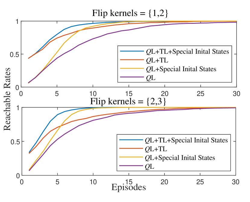
Figure 3: The learning efficiency of Algorithms 1 and 2 for finding the flip kernels of the small-scale system (18)

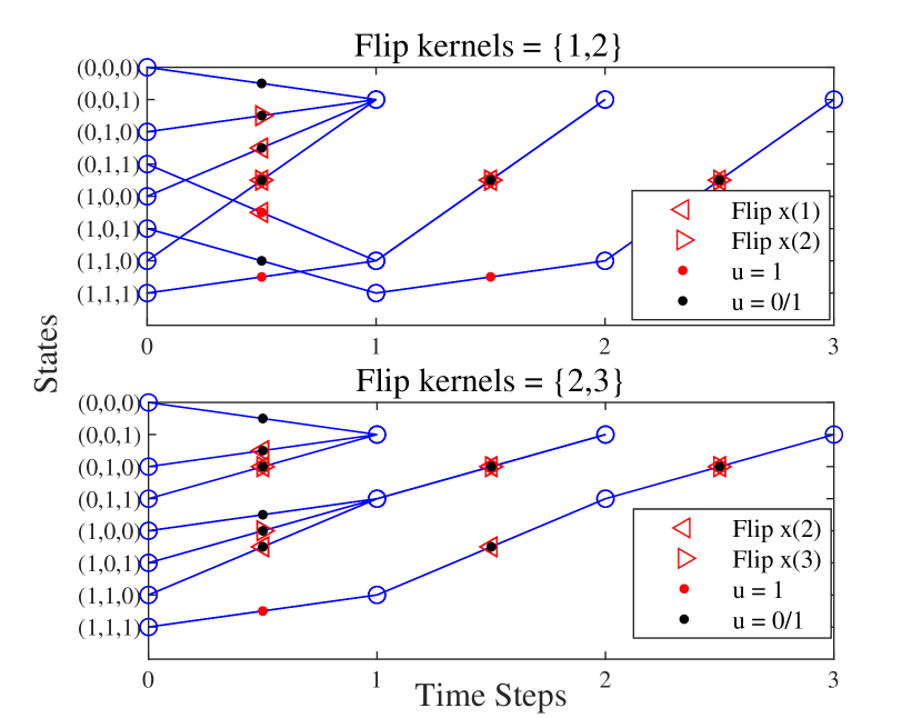
Figure 4: The optimal policy using the minimal flipping actions to realize the reachability for the small-scale system (18) obtained by Algorithm 4

$\mathbf{Remark\ 8:}$ In this paper, the system model is presented only for illustrating the problem. It should be clear that the agent has no knowledge of it.

$\mathbf{Remark\ 9:}$ The policy obtained in Figures 4 and 6 are both compared with other policies based on enumeration. It is verified that the obtained policies are both the optimal ones.

5.2 A Large-scale System

$\mathbf{Example\ 3}$: We consider the large-scale BCN with the combinational flip set $A=\{1,2,3,4,5,6\}$, the dynamics of which are given as follows:

$$\left\{\begin{aligned} x_{t+1}(1)=&x_{t}(1)\wedge(x_{t}(2)\vee x_{t}(3))\vee\neg x_{t}(1)\wedge(x_{t}(2)\oplus x_{t}(3)),\\ x_{t+1}(2)=&x_{t}(1)\vee\neg x_{t}(1)\wedge(x_{t}(2)\vee x_{t}(3)),\\ x_{t+1}(3)=&\neg(x_{t}(1)\wedge x_{t}(2)\wedge x_{t}(3)\wedge u_{t})\wedge(x_{t}(3)\vee(x_{t}(1)\vee\\ &\neg(x_{t}(2)\wedge u_{t}))\wedge(\neg x_{t}(1)\vee(x_{t}(1)\oplus x_{t}(2))\vee u_{t})),\\ x_{t+1}(3i-2)=&x_{t}(3i-2)\wedge(x_{t}(3i-1)\vee x_{t}(3i))\vee\neg x_{t}(3i-2)\wedge\\ &(x_{t}(3i-1)\oplus x_{t}(3i)),\\ x_{t+1}(3i-1)=&x_{t}(3i-2)\vee\neg x_{t}(3i-2)\wedge(x_{t}(3i-1)\vee x_{t}(3i)),\\ x_{t+1}(3i)=&x_{t}(3i)\vee(\neg x_{t}(3i-2)\vee(x_{t}(3i-2)\oplus x_{t}(3i-1))),\\ \end{aligned}\right.$$ (20)

where $i=2,3,...,9$. In terms of the reachability, we set $\mathcal{M}_{d}=(0,0,1,0,0,1,1,1,1,1,1,1,1,1,1,1,1,1,1,1,1,1,$ $1,1,1,1,1)$ and $\mathcal{M}_{0}=(a,0,0,1,0,0,1,0,0,1,0,0,1,0,0,$ $1,0,0,1,0,0,1,0,0,1)$, where $a\in\{(0,0,0),(0,1,0),(0,1,1),$ $(1,0,0),(1,0,1),(1,1,0),(1,1,1)\}$.

$\mathbf{Remark\ 10:}$ It is easy to see that the system (20) consists of 9 small-scale systems. The reason why we choose the system (20) as an example is that the optimal policy is easy to verify based on the enumeration method. It should be noted that the proposed algorithms work for all large-scale systems. The reason is listed as follows. For the agent, the system (20) and general large-scale systems are the same, due to no prior knowledge of the model.

To obtain the flip kernels of the large scale-system (20), Algorithm 3, and that with TL and special initial states are used. The efficiency of the one adding TL and special initial states is shown in Figure 5. According to Figure 5, small memory $Q$L with both TL and special initial states performs best.

Then, based on the flip kernels $\{1,2,6\}$ and $\{2,3,6\}$ obtained from Algorithm 3, the optimal policy taking the minimal flipping actions to realize the reachability is obtained by Algorithm 5, which is shown in Figure 6. It should be noted that if we set $w=2^{27}$ instead of a variable changing according to $Q=\big{|}\{x_{t}|\ Q(x_{t},.)$ is in the $Q$-table$\}\big{|}$, the policy cannot converge to the optimal one even with 10 times episodes. The above result shows the learning efficiency of Algorithm 5. In Figure 6, we simplify the state in decimal form, namely, the state $=\sum_{i=1}^{27}2^{27-i}x_{t}(i)+1$.

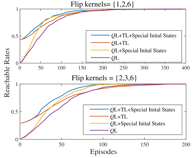
Figure 5: The learning efficiency of Algorithm 3 and it with TL and special initial states for finding the flip kernels of the large-scale system (20)

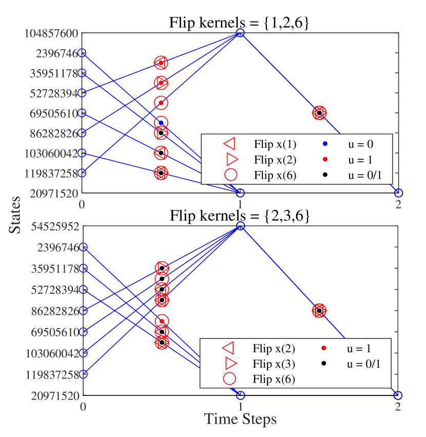
Figure 6: The optimal policy using minimal flipping actions to realize the reachability for the large-scale system (20) obtained by Algorithm 5

Table 1: Parameter settings

Example	Algorithm	$N$	$T_{max}$	$\beta$	$\omega$
2	1,2	100	10	1	0.6
3	3	$10^{4}$	$2^{27}$	1	0.6
2	4	$3\times 10^{4}$	100	0.01	0.85
3	5	$2\times 10^{5}$	$2^{27}$	0.01	0.85

Table 2: Works in this paper

Problem	Method	Advantage of the method
Flip kernels for reachability	Algorithm 1. $Q$L	Model-free, low computational complexity
	Algorithm 2. $Q$L with TL and special initial states	Higher learning efficency
	Algorithm 3. Small memory $Q$L	Applicability to large-scale systems when $|V|\times 2^{m+|B|}$ values can be stored
Minimum flipping actions for reachability	Algorithm 4. $Q$L	Model-free, low computational complexity
	Algorithm 5. Fast small memory $Q$L	Higher efficiency, applicability to large-scale systems when $|V|\times 2^{m+|B|}$ values can be stored

5.3 Details

The simulation was completed on the 6-Core Intel i5-6200U processor with a frequency of 2.30GHz, and 12GB RAM. The software we used is MATLAB R2021a.

The parameter selection is listed as follows.

• In all algorithms, we set the learning rate as a generalized harmonic series $a_{t}=\min\{1,\frac{1}{(\beta ep)^{\omega}}\}$, which satisfies conditions 1) in Lemma 1.

• In all algorithms, the greedy rate is defined as $1-\frac{0.99ep}{N}$, which decreases linearly from 1 to 0.01 as $ep$ increases.

• For Algorithms 1,2, and 3, we set $\gamma=0.99$.

• In terms of the setting of $w$, $w=8$ in Example 2 using Algorithm 3, and $w=18$ with $\Delta w=20$ in Example 3 using Algorithm 5. The above setting of $w$ ensures the optimality of the obtained policy according to Corollary 1 and Theorem 4.

According to the complexity of different Examples and Algorithms, we selected $N$, $T_{max}$, $\beta$, and $\omega$. The specific parameter settings are shown in Table 1.

6 Conclusion

In this paper, a reinforcement learning-based method is proposed to obtain minimal state-flipped control for the reachability of BCNs, which is a novel problem. The specific problems, the methods proposed and their advantages are shown in Table 2. It should be noticed that Algorithms 2,3, and 5 are novel. Some necessary and sufficient criteria have been proposed for the credibility of Algorithms 1-3. Meanwhile, we prove that the proposed reward setting can guarantee the optimal policy is obtained, under which the reachability is realized using minimal flipping actions. Finally, two examples are given to show the effectiveness of the proposed methods. It is worth noting that our approach is valid for the reachability problem of all deterministic systems with finite states.

References

- [1] S. A. Kauffman, ``Metabolic stability and epigenesis in randomly constructed genetic nets,'' Journal of theoretical biology, vol. 22, no. 3, pp. 437–467, 1969.
- [2] M. Rafimanzelat and F. Bahrami, ``Attractor controllability of Boolean networks by flipping a subset of their nodes,'' Chaos: An Interdisciplinary Journal of Nonlinear Science, vol. 28, p. 043120, 04 2018.
- [3] M. R. Rafimanzelat and F. Bahrami, ``Attractor stabilizability of Boolean networks with application to biomolecular regulatory networks,'' IEEE Transactions on Control of Network Systems, vol. 6, no. 1, pp. 72–81, 2018.
- [4] Q. Zhang, J.-e. Feng, Y. Zhao, and J. Zhao, ``Stabilization and set stabilization of switched Boolean control networks via flipping mechanism,'' Nonlinear Analysis: Hybrid Systems, vol. 41, p. 101055, 2021.
- [5] B. Chen, X. Yang, Y. Liu, and J. Qiu, ``Controllability and stabilization of Boolean control networks by the auxiliary function of flipping,'' International Journal of Robust and Nonlinear Control, vol. 30, no. 14, pp. 5529–5541, 2020.
- [6] Z. Liu, J. Zhong, Y. Liu, and W. Gui, ``Weak stabilization of Boolean networks under state-flipped control,'' IEEE Transactions on Neural Networks and Learning Systems, 2021.
- [7] Z. Liu, J. Zhong, and Y. Liu, ``Weak stabilization of k-valued logical networks,'' in 2021 40th Chinese Control Conference (CCC). IEEE, 2021, pp. 124–129.
- [8] Y. Liu, Z. Liu, and J. Lu, ``State-flipped control and q-learning algorithm for the stabilization of boolean control networks,'' Control Theory & Applications, 2021.
- [9] Z. Zhou, Y. Liu, J. Lu, and L. Glielmo, ``Cluster synchronization of Boolean networks under state-flipped control with reinforcement learning,'' IEEE Transactions on Circuits and Systems II: Express Briefs, vol. 69, no. 12, pp. 5044–5048, 2022.
- [10] R. Zhou, Y. Guo, Y. Wu, and W. Gui, ``Asymptotical feedback set stabilization of probabilistic Boolean control networks,'' IEEE transactions on neural networks and learning systems, vol. 31, no. 11, pp. 4524–4537, 2019.
- [11] H. Li and Y. Wang, ``On reachability and controllability of switched Boolean control networks,'' Automatica, vol. 48, no. 11, pp. 2917–2922, 2012.
- [12] Y. Liu, H. Chen, J. Lu, and B. Wu, ``Controllability of probabilistic Boolean control networks based on transition probability matrices,'' Automatica, vol. 52, pp. 340–345, 2015.
- [13] J. Liang, H. Chen, and J. Lam, ``An improved criterion for controllability of Boolean control networks,'' IEEE Transactions on Automatic Control, vol. 62, no. 11, pp. 6012–6018, 2017.
- [14] Watkins, P. Christopher JCH, and Dayan, ``Q-learning,'' Machine Learning, vol. 8, no. 3, pp. 279–292, 1992.
- [15] T. Jaakkola, M. Jordan, and S. Singh, ``Convergence of stochastic iterative dynamic programming algorithms,'' in Advances in Neural Information Processing Systems, vol. 6. Morgan-Kaufmann, 1993.
- [16] R. S. Sutton and A. G. Barto, Reinforcement learning: An introduction. MIT press, 2018.
- [17] D. Bertsekas, Reinforcement learning and optimal control. Athena Scientific, 2019.
- [18] A. Acernese, A. Yerudkar, L. Glielmo, and C. D. Vecchio, ``Reinforcement learning approach to feedback stabilization problem of probabilistic Boolean control networks,'' IEEE Control Systems Letters, vol. 5, no. 1, pp. 337–342, 2021.
- [19] P. Bajaria, A. Yerudkar, and C. D. Vecchio, ``Random forest Q-Learning for feedback stabilization of probabilistic Boolean control networks,'' in 2021 IEEE International Conference on Systems, Man, and Cybernetics (SMC), 2021, pp. 1539–1544.
- [20] B. Faryabi, A. Datta, and E. Dougherty, ``On approximate stochastic control in genetic regulatory networks,'' IET Systems Biology, vol. 1, pp. 361–368(7), 2007.
- [21] Y. Wu, X.-M. Sun, X. Zhao, and T. Shen, ``Optimal control of Boolean control networks with average cost: A policy iteration approach,'' Automatica, vol. 100, pp. 378–387, 2019.
- [22] Y. Wu, Y. Guo, and M. Toyoda, ``Policy iteration approach to the infinite horizon average optimal control of probabilistic Boolean networks,'' IEEE Transactions on Neural Networks and Learning Systems, vol. 32, no. 7, pp. 2910–2924, 2021.
- [23] L. Torrey and J. Shavlik, ``Transfer learning,'' in Handbook of research on machine learning applications and trends: algorithms, methods, and techniques. IGI global, 2010, pp. 242–264.
- [24] X. Peng, Y. Tang, F. Li, and Y. Liu, ``Q-learning based optimal false data injection attack on probabilistic Boolean control networks,'' Submitted.
- [25] M. Volodymyr, K. Koray, S. David, A. A. Rusu, V. Joel, M. G. Bellemare, G. Alex, R. Martin, A. K. Fidjeland, and O. a. Georg, ``Human-level control through deep reinforcement learning,'' Nature, vol. 518, no. 7540, pp. 529–533, 2015.