Conditional Adapters: Parameter-efficient
Transfer Learning with Fast Inference

Abstract

We propose Conditional Adapter (CoDA), a parameter-efficient transfer learning method that also improves inference efficiency. CoDA generalizes beyond standard adapter approaches to enable a new way of balancing speed and accuracy using conditional computation. Starting with an existing dense pretrained model, CoDA adds sparse activation together with a small number of new parameters and a light-weight training phase. Our experiments demonstrate that the CoDA approach provides an unexpectedly efficient way to transfer knowledge. Across a variety of language, vision, and speech tasks, CoDA achieves a 2x to 8x inference speed-up compared to the state-of-the-art Adapter approaches with moderate to no accuracy loss and the same parameter efficiency.

1 Introduction

Large pretrained models have achieved groundbreaking results but the main impediment to deploy them has been the cost of adaptation and inference. Due to the ever growing size of the pretrained models, for example, finetuning has become increasingly expensive as it requires a separate copy of the full model and updates to all parameters for every downstream task. Parameter-efficient transfer learning such as Adapter (Houlsby et al., 2019) and Prompt Tuning (Lester et al., 2021) have been proposed to address this issue. These methods only update a small subset of parameters for each downstream task, allowing the model to retain knowledge and avoid catastrophic forgetting (Vu et al., 2022). Noticeably, these methods can match the accuracy of a fully finetuned model, while achieving better accuracy on out-of-domain data distributions (Lester et al., 2021; Awadalla et al., 2022).

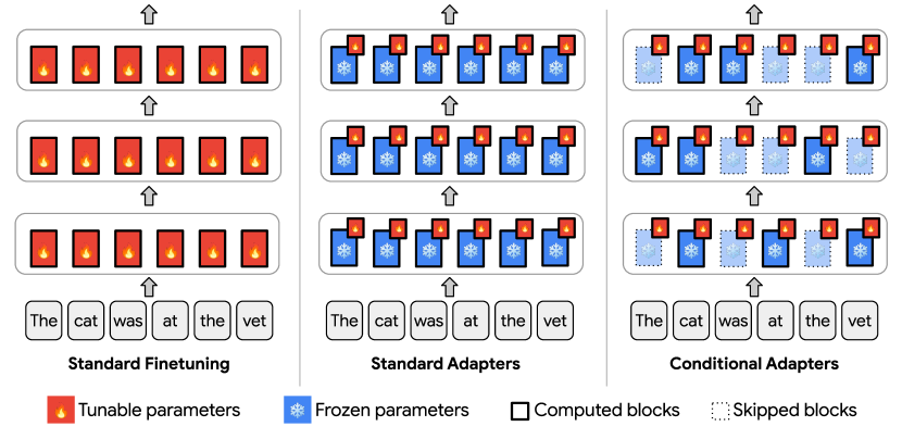
[.6] [.37] New param MNLI (text) Acc$\,\uparrow$ Speedup P-Adapter 0.4% 91.5 1.0x CoDA 0.4% 90.7 3.2x New param OCR-VQA (vision) EM$\,\uparrow$ Speedup P-Adapter 2.8% 67.5 1.0x CoDA 2.8% 67.6 8.0x New param Librispeech (speech) WER$\,\downarrow$ Speedup P-Adapter 2.5% 1.4/2.7 1.0x CoDA 2.5% 1.4/2.8 2.2x

Figure 1: Comparison between different ways to use pretrained Transformer models, including (1) standard finetuning (left) where all parameters are tunable and computation is dense, (2) standard adapters (center) where a small set of new tunable parameters are added while the computation remains dense, and (3) CoDA (right) where the computation is sparsely activated.

Figure 2: CoDA significantly reduces the inference time compared to the Parallel Adapter approach (He et al., 2021), while still maintaining parameter efficiency.

Unfortunately, standard parameter-efficient transfer learning methods only bring parameter efficiency, not inference efficiency. For example, while only a few small projection matrices are added into the pretrained model in the Adapter approach, all the model inputs (such as tokens) still use all parameters during inference. Therefore, the inference speed is the same (or slightly lower) with respect to the full finetuning method. Moreover, prior studies have shown that these parameter-efficient learning methods are most effective when the size of the pretrained model is large (Lester et al., 2021), making many advantages of these methods difficult to realize in practice.

In this paper, we propose Conditional Adapter (CoDA), a parameter-efficient transfer learning method that offers both parameter and inference efficiency. CoDA is a generalization of the adapter approach, built with the following intuition – we can treat the pretrained model as a universal source of knowledge but only query against it for necessary inputs. Figure 2 compares CoDA with finetuning and standard adapter approaches. Similar to standard adapter approaches, our model adds and updates a small adapter in each layer, while fixing the pretrained Transformer blocks for downstream adaptation. Unlike previous approaches, however, CoDA assumes that many of input token representations (of each layer) are not important for the prediction task and therefore do not require heavy computation. In such cases, the pretrained Transformer block can be skipped. Given that many tokens are not processed by the Transformer block, CoDA runs significantly faster than previous methods.

While conditional activation has clear speed benefits, CoDA must learn to select important tokens for heavy computation in order to maintain model accuracy. To this end, we introduce a soft top-$k$ operation for computing the token selection decision. This soft top-$k$ operation, which can be seen as a generalization of softmax and a relaxation of hard top-$k$, utilizes entropy-regularized optimization techniques similar to computational optimal transport (Cuturi, 2013). As a result, its output can be computed using fast and differentiable iterations, allowing token selection to be directly optimized for model performance.

We apply CoDA on encoder-heavy tasks and evaluate its effectiveness on three different domains – natural language processing, computer vision and speech processing. Overall, CoDA achieves 2 to 8 times inference speed-up over standard adapter approach with moderate to no accuracy loss. Table 2 showcases our results by selecting one of the best performing tasks in each domain. We also conduct comprehensive ablation studies to analyze the effectiveness, efficiency and scalability of CoDA. For example, we found that with just a little to no router pretraining, existing dense pretrained models such as T5 (Raffel et al., 2020) can be efficiently converted into CoDA models to gain both parameter efficiency and speed advantages.

2 Related Work

Parameter-efficient transfer learning methods

Due to the ever-growing number of parameters in the pretrained Transformer models, various methods have been proposed for transfer learning with minimal parameter updates. Prompt tuning (Lester et al., 2021) and prefix tuning (Li and Liang, 2021) introduce new virtual token embeddings that can be finetuned as model parameters. Adapter approaches (Houlsby et al., 2019; He et al., 2021) add a small number of new, learnable parameters to each layer while keeping the pretrained parameters fixed. Another popular method, Low-Rank Adaptation (LoRA; Hu et al., 2021), injects learnable low-rank decomposition matrices into pretrained model parameters. In addition to requiring less storage cost, parameter-efficient methods have been shown to be more sample-efficient and achieve better out-of-domain generalization than standard finetuning. CoDA is an adapter approach but can be easily combined with other parameter-efficient methods such as LoRA to accelerate their inference.

Conditional computation

The development of sparsely and conditionally activated models has been a very active research area. For example, Mixture-of-Experts (MoE) models (Shazeer et al., 2017) and many recent advances (Du et al., 2022; Fedus et al., 2021) have been proposed to scale up the size of language models without increasing the computation cost. Many recent works have explored better token routing methods for MoE models, for example using random hashing (Roller et al., 2021), balanced assignment (Lewis et al., 2021) and expert-choosing router (Zhou et al., 2022). CoDA applies conditional computation to both attention and feed-forward blocks of the model, whereas MoE models only focus on sparse activation in the feed-forward blocks.

Similar to our approach, various recent methods have achieved computation efficiency by skipping computation on a subset of input tokens. However, the selection mechanism can be very different, such as using pooling (Nawrot et al., 2022), token merging (Bolya et al., 2023), token pruning (Rao et al., 2021; Yin et al., 2022), learned sigmoid gates (Bapna et al., 2020) and early exiting (Schuster et al., 2022). While most of the token merging and pruning methods have been proposed for vision tasks, we show that CoDA is applicable to multiple domains including text, vision and speech. In addition, token merging and our token selection method are built with different inductive biases and intuition. Token merging leverages redundancies in visual tokens, while token selection assumes a spike of token relevance. That is, only a few tokens are necessary for the prediction task. Another major difference is that CoDA dynamically routes and updates token representations in each layer, whereas if a token is pruned (or merged), it will never be re-used by subsequent layers. We believe our token routing mechanism is more suited for text and speech applications, such as question answering, where different tokens might play important roles in different layers, or given different input queries.

Finally, CoDA is closely related to a concurrent work, CoLT5 (Ainslie et al., 2023), which also utilizes conditional activation (token selection) for inference efficiency. The focus of CoLT5 and CoDA are very different. CoLT5 specifically tailors its model architecture for long text (e.g. over 16k tokens), for example, by combining local attention with routed attention. The CoLT5 models are pre-trained from scratch and all parameters are finetuned for downstream tasks. In comparison, CoDA is directly initialized and adapted from an already pretrained dense model, and we optimize its performance on parameter-efficient transfer learning. The strengths of CoDA and CoLT5 can be combined for long text applications.

Efficient Transformer models

Many efficient Transformer variants have been proposed to accelerate model computation. Examples include creating fast attention variants (Wang et al., 2020a; Beltagy et al., 2020; Guo et al., 2022; Hua et al., 2022), searching network architectures (Press et al., 2019; So et al., 2021; Su et al., 2021) and utilizing non-attention neural modules for efficiency (Gulati et al., 2020; Lei, 2021). CoDA utilizes conditional computation as an orthogonal approach for efficiency.

Model compression

Apart from building efficient model architectures, model compression methods such as pruning (Han et al., 2016; Zhu and Gupta, 2017; Wang et al., 2020b; Xia et al., 2022) and distillation (Hinton et al., 2015; Kim and Rush, 2016; Turc et al., 2019; Lin et al., 2020) can be adopted to speed up model inference. Compared to these methods, CoDA retains all model parameters of the pretrained large model, and therefore avoids retraining a new model from scratch or knowledge forgetting caused by parameter removal. In addition, CoDA can be seen as a dynamic version of layer pruning because it can activate different Transformer layers for each token, and can be further combined with distillation to reduce the loss of accuracy caused by conditional computation.

3 Method

3.1 Architecture

Throughout this and the experiment section, we build CoDA on top of parallel adapters (He et al., 2021). However, note that our method can be generalized to other types of adapters such as sequential adapters (Houlsby et al., 2019) and LoRA (Hu et al., 2021). We present additional experimental results using LoRA in Appendix B.3. Figure 3 illustrates our architecture and shows how CoDA computes its output by selecting only a small subset of input tokens to query against the pretrained model. When parallel adapters are used, CoDA introduces a small number of learnable parameters in the parallel branches, while the vast majority of model parameters (associated with the pretrained Transformer layers) remain fixed. In addition, CoDA only sends $k=\lceil n/r\rceil$ tokens for heavy processing. We define $r>1$ as the reduction factor, a constant (such as 4) to control the computation saving.

Next, we briefly introduce our notations and describe the computation of CoDA in detail. We use $F()$ to denote a parameterized neural network and the corresponding function defined by the network. For instance, a Transformer layer (Vaswani et al., 2017) consists of an attention sub-layer $F_{\textrm{att}}()$ followed by a feed forward sub-layer $F_{\textrm{ffn}}()$. Each layer also employs layer normalization (Ba et al., 2016), namely $LN_{\textrm{att}}()$ and $LN_{\textrm{ffn}}()$, before applying the attention and feed forward functions. We define ${\bm{X}}\in{\mathbb{R}}^{n\times d}$ as the input of a Transformer encoder layer, where $n$ is the number of input tokens and $d$ is the hidden size of the model.

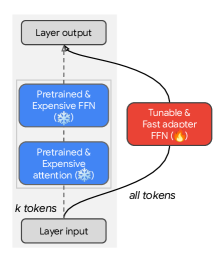
Figure 3: Illustration of a single CoDA layer with parallel adapter. $k$ tokens are selected and processed by the frozen pretrained Transformer layer, and all tokens are processed by the fast adapter layer.

Given layer input ${\bm{X}}$, we first apply layer normalization, namely ${\bm{X}}_{\textrm{norm}}=LN_{\textrm{att}}({\bm{X}})$. The normalized input will be processed by the adapter branch and the conditional Transformer branch. Their outputs are then added and combined as the final output of the layer.

Adapter branch

Let $F_{\textrm{adapter}}()$ denote the transformation function of the adapter branch. The output is defined as

$${\bm{Z}}_{\textrm{adapter}}=F_{\textrm{adapter}}({\bm{X}}_{\textrm{norm}})$$ (1)

Similar to the previous approaches, $F_{\textrm{adapter}}()$ is realized using a feed forward network with a small hidden size such as 64. As a result, computing ${\bm{Z}}_{\textrm{adapter}}$ only incurs a small number of floating point operations and its cost is often negligible compared to the cost of the heavy Transformer branch. The adapter branch does not conditionally select tokens. In other words, $F_{\textrm{adapter}}()$ is applied to all input tokens ${\bm{X}}\in{\mathbb{R}}^{n\times d}$.

Conditional branch

The computation of the conditional branch takes three steps. First, each CoDA layer defines a router function $F_{\textrm{router}}()$ to select $k$ tokens for the conditional branch. The router function in each layer returns two outputs

$${\bm{m}},{\bm{P}}=F_{\textrm{router}}({\bm{X}}_{\textrm{norm}})$$ (2)

where ${\bm{P}}\in\{0,1\}^{k\times n}$ is a matrix consisting of $k$ one-hot vectors indicating the selection of tokens. Here ${\bm{P}}[i,j]=1$ if and only if the $i$-th selected token is the $j$-th input token from $\tilde{{\bm{X}}}$. ${\bm{m}}\in[0,1]^{n}$ is a weight mask in which ${\bm{m}}[j]$ is the selection weight for the $j$-th input token. ${\bm{m}}[j]=0$ if the token is not selected. We will describe how the router learns the selection in more details later in this section.

After the routing decision is made, the input representations of the selected tokens can be collected using a matrix multiplication,

$${\bm{X}}_{\textrm{routed}} ={\bm{P}}{\bm{X}}_{\textrm{norm}}\ \ \ \ \in{\mathbb{R}}^{k\times d}$$ (3)

where $k$ rows in ${\bm{X}}_{\textrm{norm}}$ are selected to construct the $k$-by-$d$ matrix ${\bm{X}}_{\textrm{routed}}$. Similar to a standard Transformer layer, the conditional branch applies attention and feed forward transformations to the selected input:

$$\bar{{\bm{Z}}}_{\textrm{routed}} =F_{\textrm{att}}({\bm{X}}_{\textrm{routed}})$$ (4)

$${\bm{Z}}_{\textrm{routed}} =F_{\textrm{ffn}}(LN_{\textrm{ffn}}({\bm{X}}_{\textrm{routed}}+\bar{{\bm{Z}}}_{\textrm{routed}}))$$ (5)

where $\bar{{\bm{Z}}}_{\textrm{routed}},{\bm{Z}}_{\textrm{routed}}\in{\mathbb{R}}^{k\times d}$ denote the output of the attention network and the feed forward network respectively.

We consider two attention variants which differ in how they compute key-value vectors. One variant applies a $k$-to-$k$ attention using ${\bm{X}}_{\textrm{routed}}$ as both the query vectors and key-value vectors. The other variant applies a $k$-to-all attention using the entire input vectors ${\bm{X}}_{\textrm{norm}}$ as the attention keys and values. The $k$-to-all variant runs slower but obtains higher quality close to the full model. We compare the performance of the two variants in Section 5.

The attention and feed-forward output $\bar{{\bm{Z}}}_{\textrm{routed}}$ and ${\bm{Z}}_{\textrm{routed}}$ are combined and projected back to the same shape of the original input

$${\bm{Z}}_{\textrm{cond}} ={\bm{P}}^{\top}(\bar{{\bm{Z}}}_{\textrm{routed}}+{\bm{Z}}_{\textrm{routed}})\ \ \ \ \in{\mathbb{R}}^{n\times d}$$ (6)

Finally ${\bm{Z}}_{\textrm{cond}}$ merges with the adapter output and the original input of the current layer to produce the output of the layer:

$${\bm{Y}} ={\bm{X}}+{\bm{Z}}_{\textrm{adapter}}+{\bm{m}}\odot{\bm{Z}}_{\textrm{cond}}$$ (7)

${\bm{m}}\odot{\bm{Z}}_{\textrm{cond}}$ is an element-wise multiplication that scales the rows of ${\bm{Z}}_{\textrm{cond}}$ using weight ${\bm{m}}$. This operation can be seen as a gating operation, where the hidden state ${\bm{Z}}_{\textrm{cond}}[i]$ of the $i$-th token is weighted by the token selection score ${\bm{m}}[i]$ assigned by the router. This enables gradient propagation from ${\bm{m}}$ to the router parameters, such that the token selection can be jointly optimized with other model components during training.

Learned router

An important ingredient of CoDA is the router function $F_{\textrm{router}}()$ that is learned to select a subset of tokens for favorable model performance. Given the token representation ${\bm{X}}_{\textrm{norm}}$, our router first computes dot-product score ${\bm{s}}={\bm{w}}\,{\bm{X}}_{\textrm{norm}}^{\top}$, where ${\bm{w}}\in{\mathbb{R}}^{d}$ is a parameter vector associated with the router in this layer. The dot-product score ${\bm{s}}$ is further normalized by a function $f():{\mathbb{R}}^{n}\rightarrow[0,1]^{n}$, and clipped to produce the selection score ${\bm{m}}$:

$$\bm{\lambda} =f({\bm{s}})$$ (8)

$${\bm{m}} =\bm{\lambda}\odot\textrm{Top}(\bm{\lambda},k)\ \ \ \ \in{\mathbb{R}}^{n}$$ (9)

Here $\textrm{Top}(\bm{\lambda},k)\in\{0,1\}^{n}$ is an indicator function which returns a binary mask indicating the top-$k$ values in $\bm{\lambda}$. The one-hot matrix ${\bm{P}}$ defined in (2) can be created according to $\textrm{Top}(\bm{\lambda},k)$. In short, the highest values of $\bm{\lambda}$ will be selected by the router.

Function $f()$ must remain differentiable with respect to its input (${\bm{s}}$ in this case) such that we can update the router parameters ${\bm{w}}$ during training. One possible choice for $f()$ is the sigmoid activation function which normalizes the values in ${\bm{s}}$ independently. However, this does not explicitly model the constraint that we need to select $k$ tokens from $n$ available tokens. Consider a simple case where $k=1$, a natural choice for $f()$ would be the softmax function. Since softmax provides global normalization over the input scores, a gradient update to increase one of the scores would also decrease the other scores, a desirable effect for learning top-1 selection.

We hypothesize that a soft top-$k$ operator that generalizes softmax should be used for general $k>1$. This is indeed possible by formalizing soft top-$k$ as the following optimization problem:

$$f({\bm{s}})\ :=\ \operatorname*{arg\,max}_{\bm{\lambda}}\ {\bm{s}}^{\top}\bm{\lambda}+\epsilon H(\bm{\lambda})$$

$$\text{s.t.}\quad\bm{1}^{\top}\bm{\lambda}=k,\ \ \bm{\lambda}[i]\in[0,1]\ \ \forall i=1,\dots,n$$ (10)

Here $H(\bm{\lambda})=\sum_{i=1}^{n}-\bm{\lambda}[i]\log\bm{\lambda}[i]$ is a generalized entropy function (applied to any positive vector $\bm{\lambda}$ instead of a distribution), and $\epsilon>0$ is a small coefficient.

This optimization problem is closely related to the softmax and top-$k$ operation. Specifically, when $\epsilon=0$, it becomes a linear program which returns $\textrm{Top}({\bm{s}},k)$ as the solution. In addition, when $k=1$, it can be shown that its solution is $\textrm{softmax}(\bm{{\bm{s}}}/\epsilon)$. Broadly speaking, (10) will return a soft top-$k$ mask and the smoothness is controlled by $\epsilon$ (and hence $\epsilon$ must be positive to act as a temperature).

Problem (10) does not have a closed-form solution for an arbitrary $\epsilon>0$ and $k>1$, but its solution can be obtained using an iterative algorithm. Specifically, let $a\in{\mathbb{R}}$ and ${\bm{b}}\in{\mathbb{R}}^{n}$ be two auxiliary variables (which can be initialized to zeros). The solution takes the form $\bm{\lambda}=\exp(\frac{{\bm{s}}+{\bm{b}}+a}{\epsilon})$. The values of $a$ and ${\bm{b}}$ can be obtained using the following iterative updates:

$$a^{\prime} =\epsilon\ln(k)-\epsilon\ln\left(\sum_{i=1}^{n}\exp\left(\frac{{\bm{s}}[i]+{\bm{b}}[i]}{\epsilon}\right)\right)$$

$${\bm{b}}^{\prime} =\min(-{\bm{s}}-a^{\prime},0)$$ (11)

In practice, we use $T=20$ iterations and the function $f({\bm{s}})$ returns $\exp(\frac{{\bm{s}}+{\bm{b}}+a}{\epsilon})$ using $a$ and ${\bm{b}}$ from the last iteration. The function $f({\bm{s}})$ remain differentiable with respect to ${\bm{s}}$ using these iterative updates, so we can train the router jointly with other model parameters. We provide additional discussion and the derivation of the updates in Appendix §C.

3.2 Training

CoDA can be directly initialized from an existing Transformer model. Given a pretrained model such as T5 (Raffel et al., 2020), the Transformer layers are directly re-used and copied in the conditional branches of CoDA, and only the adapter and router parameters are randomly initialized. Because pretraining a large dense model can be expensive, our method reduces the overall training cost.

The routers and neural network components in CoDA must co-operate and be optimized for accurate model predictions. When the available finetuning data is limited, a random initialization for the router (and adapter) parameters can be sub-optimal. We demonstrate that CoDA can be further pretrained using the same pretraining objective as the dense model, in order to enhance downstream performance. Importantly, CoDA requires significantly fewer training steps during pretraining, since most of its parameters are taken from an already pretrained model. We show that the cost of CoDA pretraining can be 10-30x lower than the pretraining of its original dense model. We present this analysis in Section 5.

Finally, we train CoDA on downstream tasks by only updating the adapter, router and layer normalization parameters. The size of the adapters is small (e.g. 5M parameters), and each router and layer normalization block only introduces $d$ parameters, where $d$ is the model dimension. As a result, CoDA remains parameter-efficient similar to previous adapter and prompt-tuning methods.

		Base				Large				XL
Model	Reduction $r\$	MNLI	RTE	BoolQ		MNLI	RTE	BoolQ		MNLI	RTE	BoolQ	$\Delta$ Avg
Parallel Adapter	-	87.1	71.5	77.9		90.3	84.8	85.8		91.5	89.9	88.4	$\pm$0.0
(w/o conditional computation)
CoDA, $k$-to-all attention	3	86.6	72.6	76.6		90.2	85.9	85.1		91.4	91.3	89.4	$+$0.2
CoDA, $k$-to-$k$ attention		86.3	72.2	76.2		89.8	87.0	83.7		91.4	89.5	88.2	$-$0.3
CoDA, $k$-to-all attention	5	86.0	70.8	76.0		89.7	85.2	84.3		91.0	91.3	87.2	$-$0.6
CoDA, $k$-to-$k$ attention		82.5	70.8	75.4		88.1	87.0	81.8		89.9	87.7	84.8	$-$2.1

Table 1: Results of applying CoDA to T5 v1.1 models. CoDA achieves significant computation savings while retaining accuracy close to the dense baseline. We compare CoDA to a corresponding parallel adapter method that processes all tokens without conditional computation. We report accuracy on the development set on 3 tasks $\times$ 3 model sizes, and set the number of selected tokens $k=\lceil n/r\rceil$. The last column shows the change on average accuracy with respect to the parallel adapter method. We select the $k$-to-all version as our default (shown in bold).

4 Experimental setup

CoDA is evaluated on three domains including natural language processing (NLP), computer vision and speech processing, and on a range of applications such as classification, question answering, summarization and speech recognition. The experiments are organized as follows: We first demonstrate the effectivenss of CoDA conduct analyses on its design choices using the publicly available T5 models (§5). In our final results (§6), we pretrain Transformer models from scratch and extend our evaluation to vision and speech domains.

Datasets

We use the C4 corpus (Raffel et al., 2020) for pretraining text models. For speech models, we use the LibriLight corpus (Kahn et al., 2020) for pretraining. Our vision Transformer models use the same data and training procedure in Pix2Struct (Lee et al., 2022). Our finetuning datasets for text models include the MNLI (Williams et al., 2018), RTE (Dagan et al., 2005; Haim et al., 2006; Giampiccolo et al., 2007; Bentivogli et al., 2009), BoolQ (Clark et al., 2019), SQuAD (Rajpurkar et al., 2016) and XSum (Narayan et al., 2018) datasets. The speech models are evaluated on the speech recognition task using the LibriSpeech dataset (Panayotov et al., 2015). Finally, we use the OCR-VQA (Mishra et al., 2019), DocVQA (Mathew et al., 2021), and Screen2Words (Wang et al., 2021) datasets for vision models.

5 Understanding and Analyzing CoDA

Setup

We present several analyses to validate the design choices of CoDA in this section. We initialize CoDA using the version 1.1 release of T5 checkpoints, and perform CoDA pretraining using the same setting as the T5 models. During pretraining, we set routing capacity to $k=192$ given input sequence length $n=512$. We do not tune the value of $k$ for pretraining, but will report the results of using different $k$ values in finetuning. We perform 100K gradient steps, which is 10% of the total number of steps used to train the T5 dense models. The overall computational cost is over 20x less than the full training of dense models, since CoDA only applies heavy computation on less than half of the tokens.

For simplicity, we evaluate on classification tasks for various ablation studies of CoDA. Specifically, we report results on the MNLI, RTE and BoolQ datasets, and test three different model sizes including the Base, Large and XL size of T5. We will extend our evaluation to generation tasks such as question answering in the full result section (§6).

		Base				Large				XL
Model	Reduction $r\$	MNLI	RTE	BoolQ		MNLI	RTE	BoolQ		MNLI	RTE	BoolQ	$\Delta$ Avg
Soft top-$k$	3	86.3	72.2	76.2		89.8	87.0	83.7		91.4	89.5	88.2	$\pm$0.0
Sigmoid gate as $f({\bm{s}})$		85.7	70.8	72.8		89.2	82.3	81.0		90.6	88.1	86.2	$-$2.0
Truncation – selecting first $k$		81.1	70.8	72.7		84.9	77.3	82.3		85.6	84.5	85.4	$-$4.4
Soft top-$k$	5	82.5	70.8	75.4		88.1	87.0	81.8		89.9	87.7	84.8	$\pm$0.0
Sigmoid gate as $f({\bm{s}})$		82.9	71.5	72.1		86.7	82.3	80.1		88.3	87.0	82.4	$-$1.6
Truncation – selecting first $k$		62.2	64.6	71.1		64.9	70.4	75.4		66.6	76.2	81.1	$-$12.9

Table 2: Ablation study on routing methods. We use CoDA $k$-to-$k$ variant for a fair comparison with the truncation method. Better routing method delivers better accuracy on various tasks and model sizes tested. We use soft top-$k$ as our default method.

Can CoDA be fast and accurate?

Table 1 presents the finetuning results of CoDA. As a comparison, we also report the results of Parallel Adapter, which is similar to CoDA except that it applies the expensive Transformer layers to all input tokens. This constitutes an upper-bound, and is a strong baseline that has been reported as the best among a range of adapter and prompt tuning methods (He et al., 2021). As shown in Table 1, CoDA can achieve 3-5x computation reduction ($r=3,5$) in the Transformer layers at a cost of less than 1.0 point drop on average accuracy. As expected, our $k$-to-all attention variant achieves consistently better accuracy than the $k$-to-$k$ variant, since it can access the full attention context. On the other hand, the $k$-to-$k$ attention variant runs faster in practice, which can be beneficial for tasks with very long inputs. We select the $k$-to-all version in the final result section (§6).

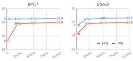
Figure 4: Finetuning accuracy (y-axis) as a function of CoDA pretraining steps (x-axis). We show results using 0, 20K, 50K and 100K pretraining steps, and for reduction factor $r=3$ and $r=5$ respectively. CoDA requires as few as 20K steps to obtain competitive finetuning accuracy.

How many pretraining steps are needed?

Figure 4 plots the finetuning accuracy by varying the number of pretraining steps for CoDA. Because CoDA can be initialized using pretrained dense models, it requires as few as 20K steps to obtain competitive finetuning results. Of course, using more pretraining steps can improve the downstream accuracy. The fact that CoDA can be quickly updated without repeating the expensive pretraining will be very beneficial in real-world applications.

Does learned routing matter?

We analyze the impact of learned routing in Table 2 by comparing our soft top-$k$ router with other router implementations. We implement a variant that replaces soft top-$k$ with the sigmoid activation function, so the selection weight of each token activates on its own (without considering the capacity constraint). As shown in the table, this variant achieves worse accuracy on almost all tasks and model sizes tested, getting 2.0 point worse on average. We also implement a “no-learning” baseline that simply selects the first $k$ tokens, which is equivalent to truncating the input sequence. This baseline performs much worse, resulting in more than 10 point decrease in accuracy for small $k$ (and equivalently large $r$). This analysis confirms the importance of learning a good routing in order to retain strong model performance.

[.76] Model Trainable Reduction  MNLI  RTE BoolQ SQuAD ReCord  XSum $\Delta$Avg Params $r$ Acc. Acc. Acc. F1 F1 R2 Parallel Adapter 10M - 91.5 91.0 88.5 94.8 91.4 21.9 $\pm$0.0 CoDA 10M 3 91.2 90.3 87.5 94.1 89.3 20.6 $-$1.0 CoDA 10M 5 90.7 89.5 87.3 93.5 87.6 20.2 $-$1.7 Prefix Tuning (Li and Liang, 2021)^† 15M (2M) - (86.3) - - - - 20.5 Sequential Adapter (Houlsby et al., 2019)^† 10M (2M) - (87.2) - - - - 20.0 Parallel Adapter (He et al., 2021)^† 10M - - - - - - 20.7 [.21]

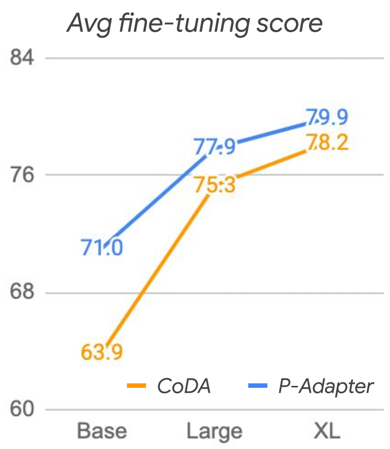
Figure 5: Comparison of CoDA and parallel adapter on 6 language tasks. We report results on the test set of XSum, and on the development set of other tasks. $\dagger$ indicates results taken from He et al. (2021), and referenced results in bracket correspond to using 2M adapter parameters. Note that our Parallel Adapter numbers are stronger as our pretrained Transformer backbone uses more parameters than the model used in He et al. (2021).

Figure 6: Average finetuning scores of Parallel Adapter and CoDA at different model sizes.

6 Full Results

Setup

In this section, we apply our best training recipe to all tasks and application domains. We first pretrain dense Transformer models, followed by the CoDA training procedure in §3.2. Our speech models are pretrained using a masked language modeling (MLM) objective similar to BERT (Devlin et al., 2019), and random quantized output label space (Chiu et al., 2022). Our vision and text models use an encoder-decoder architecture similar to T5 but incorporate a few changes. Following PaLM (Chowdhery et al., 2022), we use multi-query attention (Shazeer, 2019) that shares the same key and value projection for multiple query heads. We only use 6 decoder layers and increase the feed forward hidden size (to compensate for the decrease in the number of layers). These modifications have a neutral effect on model quality, but speed up auto-regressive decoding significantly. We will show CoDA is compatible with these changes and can further speed up inference by a considerably large factor. We provide more details of our experimental setup in Appendix A.

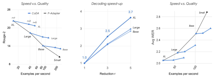
Figure 7: The scaling of CoDA on the XSum and LibriSpeech dataset. Left: CoDA achieves better speed-quality trade-off than finetuning adapters with smaller models, on the XSum dataset. Middle: larger CoDA model achieves higher speed-ups. Right: CoDA achieves better speed-quality trade-off than the dense baseline on the LibriSpeech dataset.

NLP results

In addition to the classification datasets used in Section 5, we also evaluate our final models on the SQuAD, ReCord and XSum datasets which require generating an answer or a summary given the input. Table 6 contains the finetuning results of XL models. Compared to the parallel adapter baseline that uses full computation, CoDA achieves 3x and 5x computation reduction with only 1.0 and 1.7 point loss in average score.

Figure 6 and 7 highlight the scaling trend of CoDA. CoDA runs much faster with slightly worse quality than the parallel adapter baseline. This is expected because the baseline processes all tokens in every layer, whereas CoDA only selects $1/r$ of tokens for heavy processing. Importantly, this quality gap reduces as the model size increases (as shown in Figure 6), making CoDA a computationally efficient choice for large models. Indeed, CoDA can trade off quality for speed by varying the number of selected tokens. Figure 7 (left) demonstrates that CoDA achieves much stronger speed-quality trade-off compared to dense models without conditional computation. The black line indicates the results of Parallel Adapter when the model size grows from Small to XL, and each blue line represents the speed-quality trade-off of CoDA using $r=1,3,5$. Moreover, Figure 7 (middle) shows that larger CoDA models exhibit higher inference speed-ups. These observations are consistent on other tasks. We provide additional results in Appendix §B.

[.47] Model $r$ Base Large XL clean other clean other clean other w2v-BERT - 1.8 3.6 1.5 2.9 1.5 2.9 BEST-RQ - 1.7 3.5 1.6 2.9 1.4 2.7 P-Adapter - 1.6 3.5 1.4 3.0 1.4 2.7 CoDA 2 1.6 3.5 1.4 3.0 1.4 2.8 CoDA 4 1.6 3.6 1.5 3.1 1.4 2.8 [.49] Model $r$ OCRVQA DocVQA Screen2Words EM Speedup ANLS Speedup CIDEr Speedup Parallel Adapter - 67.5 1$\times$ 70.8 1$\times$ 110.2 1$\times$ CoDA 4 68.2 4.6$\times$ 71.8 4.6$\times$ 111.6 4.6$\times$ CoDA 8 67.6 8.0$\times$ 66.6 8.0$\times$ 108.1 8.0$\times$ CoDA 16 66.9 13.5$\times$ 56.6 12.1$\times$ 109.0 12.5$\times$ CoDA 32 64.4 19.4$\times$ 42.5 16.7$\times$ 104.2 17.8$\times$

Figure 8: Comparison of CoDA and the parallel adapter baselines on Librispeech. We report the WER results on test-clean and test-other. More results can be found in §B.2.

Figure 9: Comparison of CoDA and the parallel adapter applied to a pretrained Pix2Struct model (Lee et al., 2022) on 3 visually-situated language understanding tasks.

Speech recognition results

We further validate the performance of CoDA in the speech domain. Our model uses a Transformer encoder and a 2-layer LSTM Transducer (Graves, 2012). Similar to NLP setups, we test the performance of the speech model on 3 scales – Base, Large and XL (see Appendix A for details). Table 9 demonstrates that with sizable reduction ratios ($r=2,4$), the change on word error rate (WER) is consistently minimal on the test-clean and test-other sets of LibriSpeech across different model sizes (and on other sets in §B.2). Moreover, our results are comparable to the top-performing models, such as w2v-BERT (Chung et al., 2021) and BEST-RQ (Chiu et al., 2022), that are fully finetuned by updating all parameters. Figure 7 (right) highlight again that applying conditional computation leads to better speed-quality trade-off compared to dense models.

Original Image	Layer 0	Layer 8	Layer 17

Figure 10: Visualization of routing preferences for a CoDA model applied to the OCR-VQA task. Warmer and cooler colors represent higher and lower scores respectively. Router prefers diverse coverage in early layers, but converges to selecting sparse and representative patches in later layers.

Vision results

We extend our experiments to visual tasks that involves natural language within the image, such as documents and user interfaces. Our experiments are based on Pix2Struct (Lee et al., 2022), where an image-encoder-text-decoder is pretrained by learning to predict simplified HTML from webpage screenshots. Table 9 shows the results on three tasks that were also evaluated in the original Pix2Struct paper. In OCRVQA and Screen2Words, we observe relatively small drops in performance when reducing the number of routed tokens (i.e. patches). When the capacity is 1/16th of the original sequence length, leading to around 13$\times$ speedup, we only lose about 1 point. We speculate that this is due to the high-level sparsity in the inputs for these two tasks. For DocVQA, where there is comparatively more textual information, we observe a steeper performance-speed trade-off but still achieve a 8$\times$ speedup with a 4-point drop.

To provide a more intuitive understanding why CoDA works, we visualize the router behavior for the OCR-VQA model in Figure 10. We show which patches the routers prefers the most (warmest colors) and least (coolest colors), for several layers. The first, immediately obvious, observation is that router avoids low-frequency patches, i.e. patches likely to be “whitespace”, since they can be adequately handled by the cheap adapter layers. The second, more subtle, observation is that the router progressively converges on a small number of key patches that we hypothesize serve as representations for larger regions. The visualization confirms that CoDA is able to select meaningful and representative patches that are useful for the prediction task.

7 Conclusion and Limitation

We present CoDA, a parameter-efficient adapter method that enables fast inference. CoDA relies on conditional computation to selectively activate model computation on important input units, providing a novel way to balance model expressivity and efficiency.

In this work, we focus on encoder-heavy applications such as summarization, speech recognition and visual question answering, by applying our method to the encoder. One limitation of CoDA is that the current routing mechanism (i.e. token selection in a given sequence) is not directly applicable to decoder-only models for auto-regressive token generation. Enabling fast token generation using conditional activation in decoder layers is an interesting direction we plan to explore in future work.

8 Acknowledgements

We would like to thank Rama Pasumarthi, Hongkun Yu, Kelvin Guu, Zhuyun Dai, Timothy Dozat, Raphael Hoffmann, Tao Wang, Tal Schuster, Ziwei Ji, Frederick Liu and Slav Petrov for helpful advice and discussion.

Appendix A Experimental details

Model implementation

For our text and vision experiments, we implement our models using JAX [Bradbury et al., 2018]. Specifically, our training and model modules are built on top of the T5X, Flax and Flaxformer framework [Roberts et al., 2022, Heek et al., 2020]. Following the T5 v1.1 implementation and PaLM [Chowdhery et al., 2022], our Transformer models use the GLU variant [Shazeer, 2020] as the feed forward network and multi-query-attention [Shazeer, 2019] as the attention block. These modifications are shown to enhance modeling capacity and speed up decoding respectively.

For the speech experiments, we use TensorFlow [Abadi et al., 2015] and the Lingvo framework [Shen et al., 2019]. The state-of-the-art Transformer variant for speech recognition is the Conformer architecture [Gulati et al., 2020] which additionally uses depth-wise convolution in each layer. Since the convolution operation is applied to consecutive inputs and does not immediately support routing, we use the standard Transformer architecture [Vaswani et al., 2017] instead. Swish activation is used in the feed forward blocks, following Gulati et al. [2020]. We provide the model configuration details in Table 3.

Model	Num of params	Layers	Num of heads	$d_{\textrm{model}}$	$d_{\textrm{ffn}}$	$d_{\textrm{head}}$	$d_{\textrm{adpt}}$
Text Base	0.1B	12, 6	12	768	3072	128	64
Text Large	0.5B	24, 6	16	1024	4096	128	64
Text XL	2.1B	24, 6	32	2048	8192	128	64
Speech Base	0.2B	31, 2	8	768	3072	96	256
Speech Large	0.6B	32, 2	8	1280	5120	160	256
Speech XL	1.1B	32, 2	8	1664	6656	208	256
Vision	0.7B	18, 6	24	1536	3968	128	256

Table 3: Configuration of Transformer models used in §6. We show the total number of parameters (in billions). $d_{\textrm{model}}$ is the model hidden dimension, $d_{\textrm{ffn}}$ is the intermediate FFN hidden dimension, $d_{\textrm{head}}$ is the attention head dimension and $d_{\textrm{adpt}}$ is the adapter hidden dimension.

Dataset	Input length	Batch size	Steps	Optimizer	Learning rate
MNLI	128	128	300K	Adafactor	0.001, constant
RTE	256
BoolQ	384
SQuAD	512
ReCord	512
XSum	1664
LibriSpeech	3200	256	150K	Adafactor	0.001, inverse decay
OCR-VQA	4096	256	20K	Adafactor	0.01, cosine decay
DocVQA	4096	256
Screen2Words	4096	32

Table 4: Fine-tuning hyperparmaeters. We use a maximum of 300K steps for NLP tasks following T5 [Raffel et al., 2020]. Pix2struct [Lee et al., 2022] uses 10K fine-tuning steps for vision tasks. We use 20K steps as CoDA takes longer to train.

Model training

We use the same data and procedure described in T5 [Raffel et al., 2020], BEST-RQ [Chiu et al., 2022] and Pix2struct [Lee et al., 2022] for pre-training the respective text, speech and vision models. We use the same training hyper-parameters, such as batch size, input sequence length, the number of pre-training steps and the choice of optimizer and learning rate scheduling. All models have been pre-trained using 128 or 256 TPUv3/TPUv4 chips.

We run CODA pre-training for text and vision models, using an additional 100K steps and 200K steps respectively. For text models, the input sequence length is $n=512$ and we set the number of selected tokens $k=192$. For vision models, the input sequence contains $n=4096$ image patches and we set $k=1024$. CODA pre-training is not used for our speech models because there are sufficient fine-tuning data. Following standard practice in speech, we use the 1K hour data from the LibriSpeech dataset [Panayotov et al., 2015] and another 30K hour data generated using the noisy student self-training method [Xie et al., 2020, Zhang et al., 2022].

Table 4 lists the hyper-parameters used for fine-tuning, including the sequence length, learning rate, batch size and the number of fine-tuning steps used. For NLP datasets, we set the maximum input length and decoding length to the 98th percentile of lengths in the training set. For vision datasets, we set the input length following the suggested values in Pix2struct. We also find that annealing the number of routed tokens $k$ can achieve better finetuning results. Specifically, we decrease $k$ linearly from the sequence length $n$ down to the target value $n/r$ using the first $10\%$ to $20\%$ of the finetuning steps.

Appendix B Additional results

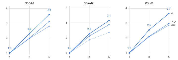
(a)

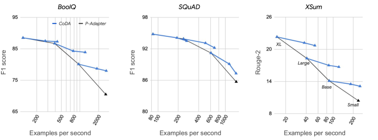
(b)

Figure 11: Analyzing the speed and quality of CoDA. We select 3 representative tasks including BoolQ (classification), SQuAD (question answering) and XSum (summarization). (a) Relative decoding speed given different reduction factor $r$. (b) Speed-quality trade-off of CoDA applied on different tasks and model sizes. CoDA achieves better quality than the dense Parallel Adapter baseline when running at a similar inference speed. The black line shows the performance of Parallel Adapter given Small to XL model size. Each blue line represents the performance of CoDA for reduction $r=1,3,5$ for a given model size. When $r=1$, CoDA is equivalent to the dense baseline.

Model	Trainable	Reduction		MNLI	RTE	BoolQ	SQuAD	ReCord	XSum
	Params	$r$		Acc.	Acc.	Acc.	F1	F1	R2
				Base
Parallel Adapter	2M	-		88.2	75.8	80.1	91.2	76.7	14.1
CoDA		3		85.8	68.6	78.7	89.1	69.1	13.5
CoDA		5		82.8	60.3	78.0	87.3	61.8	13.1
				Large
Parallel Adapter	5M	-		90.5	90.6	86.7	93.9	87.2	18.3
CoDA		3		90.0	84.8	84.3	93.1	84.6	17.0
CoDA		5		89.4	88.5	83.9	92.2	81.2	16.7
				XL
Parallel Adapter	10M	-		91.5	91.0	88.5	94.8	91.4	22.3
CoDA		3		91.2	90.3	87.5	94.1	89.3	21.2
CoDA		5		90.7	89.5	87.3	93.5	87.6	20.7

Table 5: Fine-tuning results on 6 language tasks $\times$ 3 model sizes. We report the best results on the development set.

B.1 NLP

Table 5 contains the complete fine-tuning results on the 6 language datasets. As discussed in §6, the gap between CoDA and its counterpart without conditional computation is large at Base size. As the model size increases, CoDA retains almost the same level of quality given 3x computation reduction ($r=3$). The reduction leads to decoding speed-ups, as shown in Figure 11. More importantly, we see that larger model benefits more from CoDA, achieving a speed-up factor close to the reduction factor $r$. These results highlight the potential of CoDA for large-scale models, which we plan to investigate in future work.

Model	$r$	Base						Large						XL					$\Delta$ Avg
		dev			test			dev			test			dev			test
		clean	other		clean	other		clean	other		clean	other		clean	other		clean	other
w2v-BERT	-	1.7	3.6		1.8	3.6		1.5	2.9		1.5	2.9		1.5	2.6		1.5	2.9	-
BEST-RQ	-	1.6	3.5		1.7	3.5		1.5	2.8		1.6	2.9		1.4	2.7		1.4	2.7	-
Parallel Adapter	-	1.5	3.5		1.6	3.5		1.4	3.0		1.4	3.0		1.4	2.7		1.4	2.7	$\pm$0.0
CoDA	2	1.5	3.5		1.6	3.5		1.4	3.0		1.4	3.0		1.4	2.7		1.4	2.8	$+$0.01
CoDA	4	1.6	3.6		1.6	3.6		1.4	3.1		1.5	3.1		1.4	2.8		1.4	2.8	$+$0.07

Table 6: Comparison of CoDA and the parallel adapter baselines on all 4 splits (dev-clean, dev-other, test-clean, test-other) of Librispeech.

B.2 Speech

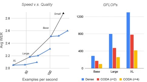
Figure 12: The scaling of CoDA on Librispeech. Left: Larger models with CoDA can achieve much better performance with the same or faster speed compared to smaller models. Right: GFLOPS reduction is significant as $r$ increases.

Table 6 extends Table 9 by including WER results on dev-clean and dev-other splits. From the table, one can observe that XL with CoDA ($r=2,4$) are consistently better than the Large parallel adapter model on each split, and the Large model with CoDA ($r=2,4$) are also consistently better than the Base PA on each split. Given the inference speeds for CoDA models shown in Table 12, larger CoDA models are generally faster and better than smaller dense ones (even with PA) with regard to either time cost or computation GFLOPs. Therefore, it is likely for CoDA to help scale up ASR models with decent computation resources and time cost.

B.3 Combining CoDA and LoRA

CoDA can be easily combined with other types of adapter methods. To see this, we additionally implemented a variant that combines with Low-Rank Adapter [LoRA; Hu et al., 2021], which is another parameter-efficient transfer learning method that recently became the most popular choice for LLMs. We incorporate the latest development suggested in the QLoRA paper [Dettmers et al., 2023], which adds low-rank adapters to every linear projection matrix in the Transformer layers. This is found to obtain better fine-tuning performance than the original implementation. Our CoDA variant with LoRA simply removes the parallel adapter branches and instead adds low-rank adapters to the projection matrices of the pretrained layers.

Table 7 shows the finetuning results. The new LoRA baseline achieves stronger accuracy than the Parallel Adapter baseline (84.0 v.s. 82.9 on average), highlighting the effectiveness of recent development on LoRA. In addition, our CoDA variant using LoRA still achieves very close accuracy compared to its dense counterpart (84.0 v.s. 84.0 or 83.7 on average). We believe the additional results strengthen our claims – that CoDA enables a strong trade-off between accuracy and efficiency using conditional activation, and this technique can be combined with other developments in PETL.

		Base				Large
Model	Reduction $r\$	MNLI	RTE	BoolQ		MNLI	RTE	BoolQ	Avg on 6
Parallel Adapter (PA)	-	87.1	71.5	77.9		90.3	84.8	85.8	82.9
CoDA w/ PA	3	86.6	72.6	76.6		90.2	85.9	85.1	82.8
CoDA w/ PA	5	86.0	70.8	76.0		89.7	85.2	84.3	82.0
Low-rank Adapter (LoRA)	-	88.0	73.7	80.3		90.7	85.2	86.3	84.0
CoDA w/ LoRA	3	86.2	76.9	78.4		90.3	86.3	85.8	84.0
CoDA w/ LoRA	5	86.0	76.9	78.3		89.8	86.3	84.7	83.7

Table 7: Results of applying CoDA with Parallel Adapter v.s. Low-Rank Adapter. We report results on the development sets and on the Base and Large model size.

Appendix C Soft top-$k$ algorithm

C.1 Derivation of the iterative updates

We present the derivation of iterative updates (11) for solving the soft top-$k$ problem (10) in Section 3. The soft top-$k$ operation is defined as a maximization problem (10). For the derivation, we rewrite it as an equivalent minimization problem:

$$\max_{\bm{\lambda}}\ \ {\bm{s}}^{\top}\bm{\lambda}+\epsilon H(\bm{\lambda})$$

$$\Longleftrightarrow\qquad \min_{\bm{\lambda}}\ \ -{\bm{s}}^{\top}\bm{\lambda}-\epsilon H(\bm{\lambda})$$

$$\Longleftrightarrow\qquad \min_{\bm{\lambda}}\ \ -{\bm{s}}^{\top}\bm{\lambda}-\epsilon H(\bm{\lambda})-\epsilon\bm{1}^{\top}\bm{\lambda}$$ (12)

s.t. $$\bm{1}^{\top}\bm{\lambda}=k,\ \ \bm{\lambda[i]}\in[0,1],\ \ i=1,\dots,n.$$

Note the term $\epsilon\bm{1}^{\top}\bm{\lambda}$ will be a constant $\epsilon\times k$, but we include it in the minimization object to make our derivation simpler later.

Now, let $a\in\mathbb{R}$ and ${\bm{b}}\in\mathbb{R}^{m}$ be the Lagrangian variables corresponding to the linear constraints $\bm{1}^{\top}\bm{\lambda}=k$ and $\bm{\lambda}[i]\leq 1\ \forall i\$. The minimization problem is equivalent to its Lagrangian expression:

$$\min_{\lambda\in\mathbb{R}^{m}}\ \max_{a\in\mathbb{R},{\bm{b}}\leq\bm{0}}\ -{\bm{s}}^{\top}\bm{\lambda}-\epsilon H(\bm{\lambda})-\epsilon\bm{1}^{\top}\bm{\lambda}+a(k-\bm{1}^{\top}\bm{\lambda})+\bm{b}^{\top}(\bm{1}-\bm{\lambda})$$ (13)

The objective function (12) is strongly convex and the solution space of $\bm{\lambda}$ is a convex set. As a result, strong duality holds so we can instead solve the dual problem. The dual problem exchanges the $\min$ and $\max$ operators in (13):

$$\max_{a\in\mathbb{R},{\bm{b}}\leq\bm{0}}\ \min_{\lambda\in\mathbb{R}^{m}}\ -{\bm{s}}^{\top}\bm{\lambda}-\epsilon H(\bm{\lambda})-\epsilon\bm{1}^{\top}\bm{\lambda}+a(k-\bm{1}^{\top}\bm{\lambda})+\bm{b}^{\top}(\bm{1}-\bm{\lambda})$$ (14)

The optimal solution $(a,{\bm{b}},\bm{\lambda})$ must have the Karush-Kuhn-Tucker (KKT) conditions hold [Kuhn and Tucker, 2014], namely

$$\frac{\partial\left(-{\bm{s}}^{\top}\bm{\lambda}-\epsilon H(\bm{\lambda})+\epsilon\bm{1}^{\top}\bm{\lambda}+a(k-\bm{1}^{\top}\bm{\lambda})+\bm{b}^{\top}(\bm{1}-\bm{\lambda})\right)}{\partial\bm{\lambda}}=0$$

$$\Longleftrightarrow\qquad \bm{\lambda}=\exp\left(\frac{{\bm{s}}+a+{\bm{b}}}{\epsilon}\right)\quad\Longleftrightarrow\quad\bm{\lambda}[i]=\exp\left(\frac{{\bm{s}}[i]+a+{\bm{b}}[i]}{\epsilon}\right)\ \ \forall i=1,\dots,n$$

Substituting $\bm{\lambda}$ using the above equation in (14), the dual problem now has a simple form:

$$\max_{a\in\mathbb{R},{\bm{b}}\leq\bm{0}}k\cdot a+\bm{1}^{\top}{\bm{b}}-\bm{1}^{\top}\exp\left(\frac{{\bm{s}}+a+{\bm{b}}}{\epsilon}\right)$$

We can solve this problem using coordinate descent [Wright, 2015] by successively maximizing the function with either $a$ or ${\bm{b}}$ fixed. That is, we find the optimal $a$ that maximizes the dual objective given a fixed ${\bm{b}}$, and vice versa. This leads to the iterative updates (11) described in Section 3.

$$\begin{split}a^{\prime}=\epsilon\ln(k)-\epsilon\ln\left(\sum_{i=1}^{n}\exp\left(\frac{{\bm{s}}[i]+{\bm{b}}[i]}{\epsilon}\right)\right),\qquad\qquad{\bm{b}}^{\prime}=\min(-{\bm{s}}-a^{\prime},0)\end{split}$$

In short, we obtain the iterative updates of the soft top-$k$ problem (10) by solving its dual problem and by performing coordinate decent of the dual variables $a$ and ${\bm{b}}$. The iterative updates are in fact the coordinate decent steps.

C.2 The $\epsilon$-scaling trick

The iterations of $a$ and ${\bm{b}}$ will converge but the number of iterations needed can be very large for small $\epsilon$. In practice, we only perform a small number of iterations and return the corresponding $\bm{\lambda}$, which may be close but not the exact solution to (12). In order to improve the convergence given a small number of iterations, we apply an empirical trick called the $\epsilon$-scaling heuristic [Schmitzer, 2019]. Let $\epsilon_{t}$ denote the value of $\epsilon$ at the $t$-th iteration. We initialize $\epsilon_{0}$ to a larger value and gradually reduce $\epsilon_{t}$ to the target $\epsilon$. Specifically, we set $\epsilon_{t}=\max(\beta\epsilon_{t-1},\epsilon)$ at the $t$-th iteration, using a scaling constant $\beta\in(0,1)$. We use $\epsilon_{0}=4$ throughout our experiments, $\epsilon=0.03$ and $\beta=0.7$ for text and vision models and $\epsilon=1.0$ and $\beta=0.85$ for speech models. Using a larger number of iterations leads to better convergence but we found $T=20$ sufficient for our experiments.

C.3 Overhead of soft top-$k$ iterations

The soft top-$k$ iterations are performed for every routed Transformer layer. Although this seems computationally expensive, the actual overhead is very small compared to the overall decoding latency. The complexity only scales linearly with the number of layers and the sequence length, and does not depend on the model dimension $d$. Table 8 showcases the latency numbers on the BoolQ and XSum datasets, when performing batched decoding using a single TPUv4 chip. We observe that the cost of iterations is less than 2% of the total decoding latency. Moreover, the relative cost decreases dramatically as the model size increases, since it does not depend on the model dimension.

Task	Model size	Iteration latency (ms)	Total latency (ms)
BoolQ	Base	0.9	48.0
	Large	1.7	105.3
	XL	1.7	297.6
XSum	Base	1.0	513.9
	Large	2.0	1076.2
	XL	2.0	2426.0

Table 8: Latency (in milliseconds) of the soft top-$k$ iteration and the total decoding time per batch. We use a single TPUv4 chip and 128 sequences per batch. The maximum iteration overhead is less than 2% of the total latency.

C.4 Additional discussion

This iterative algorithm is closely related to the Sinkhorn algorithm of Optimal Transport (OT). Specifically, the Sinkhorn algorithm solves the entropy-regularized version of Optimal Transport [Cuturi, 2013]. However, our work concerns an different optimization instance. While OT solves a transportation problem where the solution space is defined with the marginal constraints over the rows and columns of a transportation matrix, our optimization problem is constrained with a total budget ($\sum_{i}\lambda_{i}=k$) and upper bounds ($\lambda_{i}\leq 1\ \forall i$). This leads to different iterative updates.

Concurrent to our work, Tai et al. [2022] have used a similar linear program (LP) formulation for soft top-$k$ operation, and have applied the operator for learning sparse neural networks (i.e. model pruning). Compared to our formulation (12), they first reduce the LP to an equivalent instance of optimal transport problem, before introducing the entropy term. As a result, the derived updates are different. In addition, Tai et al. [2022] have introduced an initialization for the dual variables to improve the convergence of their algorithm, whereas we use $\epsilon$ scaling instead. Their implementation can be explored for CoDA as well.

Besides formulating soft top-$k$ using entropy-regularized optimization, there are other possible variants for trainable sparsity. One example is sparsemax [Martins and Astudillo, 2016] that can learn sparse multi-label probabilities. We believe that the sparsemax formulation can generalize from the top-1 to top-$k$ case, but it is beyond the scope of this work. We use the current soft top-$k$ implementation because it is a natural extension of softmax (see discussions in §3), and because it can be solved using simple iterative updates.

Appendix D Author Contributions

All authors have contributed to running experiments and discussing research ideas. Tao leads the project, developed the conditional architecture, designed the experiments and analyses. Kenton, Yu and Ming-Wei proposed the idea of applying conditional computation for large model adaptation. Joshua demonstrated the conditional architecture is applicable to attention, and implemented the initial version of conditional attention block. Tao, Yanqi, Nan, Vincent, Yuexin, Ming-Wei and Yu conducted the NLP experiments including model pre-training, fine-tuning and various ablation analyses. Siddhartha conducted the majority of the vision experiments. Kenton conducted the vision analysis and advised on the vision experiments. Junwen conducted the majority of the speech experiments. Bo and Yu assisted in trouble-shooting the speech models, ran the model pre-training and provided guidance on the speech experiments. Finally, Tao, Ming-Wei, Junwen and Kenton made the primary contributions to the writing of the paper.

References

- Abadi et al. (2015) Martín Abadi, Ashish Agarwal, Paul Barham, Eugene Brevdo, Zhifeng Chen, Craig Citro, Greg S. Corrado, Andy Davis, Jeffrey Dean, Matthieu Devin, Sanjay Ghemawat, Ian Goodfellow, Andrew Harp, Geoffrey Irving, Michael Isard, Yangqing Jia, Rafal Jozefowicz, Lukasz Kaiser, Manjunath Kudlur, Josh Levenberg, Dandelion Mané, Rajat Monga, Sherry Moore, Derek Murray, Chris Olah, Mike Schuster, Jonathon Shlens, Benoit Steiner, Ilya Sutskever, Kunal Talwar, Paul Tucker, Vincent Vanhoucke, Vijay Vasudevan, Fernanda Viégas, Oriol Vinyals, Pete Warden, Martin Wattenberg, Martin Wicke, Yuan Yu, and Xiaoqiang Zheng. TensorFlow: Large-scale machine learning on heterogeneous systems, 2015. URL https://www.tensorflow.org/. Software available from tensorflow.org.
- Ainslie et al. (2023) Joshua Ainslie, Tao Lei, Michiel de Jong, Santiago Ontañón, Siddhartha Brahma, Yury Zemlyanskiy, David Uthus, Mandy Guo, James Lee-Thorp, Yi Tay, et al. Colt5: Faster long-range transformers with conditional computation. In Proceedings of the 2023 Conference on Empirical Methods in Natural Language Processing (EMNLP), 2023.
- Awadalla et al. (2022) Anas Awadalla, Mitchell Wortsman, Gabriel Ilharco, Sewon Min, Ian Magnusson, Hannaneh Hajishirzi, and Ludwig Schmidt. Exploring the landscape of distributional robustness for question answering models. arXiv preprint arXiv:2210.12517, 2022.
- Ba et al. (2016) Jimmy Lei Ba, Jamie Ryan Kiros, and Geoffrey E Hinton. Layer normalization. arXiv preprint arXiv:1607.06450, 2016.
- Bapna et al. (2020) Ankur Bapna, Naveen Arivazhagan, and Orhan Firat. Controlling computation versus quality for neural sequence models. arXiv preprint arXiv:2002.07106, 2020.
- Beltagy et al. (2020) Iz Beltagy, Matthew E. Peters, and Arman Cohan. Longformer: The long-document transformer. arXiv:2004.05150, 2020.
- Bentivogli et al. (2009) Luisa Bentivogli, Peter Clark, Ido Dagan, and Danilo Giampiccolo. The fifth pascal recognizing textual entailment challenge. In TAC, 2009. URL https://tac.nist.gov/publications/2009/additional.papers/RTE5_overview.proceedings.pdf.
- Bolya et al. (2023) Daniel Bolya, Cheng-Yang Fu, Xiaoliang Dai, Peizhao Zhang, Christoph Feichtenhofer, and Judy Hoffman. Token merging: Your ViT but faster. In International Conference on Learning Representations, 2023.
- Bradbury et al. (2018) James Bradbury, Roy Frostig, Peter Hawkins, Matthew James Johnson, Chris Leary, Dougal Maclaurin, George Necula, Adam Paszke, Jake VanderPlas, Skye Wanderman-Milne, et al. Jax: composable transformations of python+ numpy programs. Version 0.2, 5:14–24, 2018.
- Chiu et al. (2022) Chung-Cheng Chiu, James Qin, Yu Zhang, Jiahui Yu, and Yonghui Wu. Self-supervised learning with random-projection quantizer for speech recognition. In Kamalika Chaudhuri, Stefanie Jegelka, Le Song, Csaba Szepesvari, Gang Niu, and Sivan Sabato, editors, Proceedings of the 39th International Conference on Machine Learning, volume 162 of Proceedings of Machine Learning Research, pages 3915–3924. PMLR, 17–23 Jul 2022. URL https://proceedings.mlr.press/v162/chiu22a.html.
- Chowdhery et al. (2022) Aakanksha Chowdhery, Sharan Narang, Jacob Devlin, Maarten Bosma, Gaurav Mishra, Adam Roberts, Paul Barham, Hyung Won Chung, Charles Sutton, Sebastian Gehrmann, et al. Palm: Scaling language modeling with pathways. arXiv preprint arXiv:2204.02311, 2022.
- Chung et al. (2021) Yu-An Chung, Yu Zhang, Wei Han, Chung-Cheng Chiu, James Qin, Ruoming Pang, and Yonghui Wu. W2v-bert: Combining contrastive learning and masked language modeling for self-supervised speech pre-training. In 2021 IEEE Automatic Speech Recognition and Understanding Workshop (ASRU), pages 244–250. IEEE, 2021.
- Clark et al. (2019) Christopher Clark, Kenton Lee, Ming-Wei Chang, Tom Kwiatkowski, Michael Collins, and Kristina Toutanova. BoolQ: Exploring the surprising difficulty of natural yes/no questions. In Proceedings of the 2019 Conference of the North American Chapter of the Association for Computational Linguistics: Human Language Technologies, Volume 1 (Long and Short Papers), 2019. URL https://aclanthology.org/N19-1300.
- Cuturi (2013) Marco Cuturi. Sinkhorn distances: Lightspeed computation of optimal transport. Advances in neural information processing systems, 26, 2013.
- Dagan et al. (2005) Ido Dagan, Oren Glickman, and Bernardo Magnini. The pascal recognising textual entailment challenge. In Proceedings of the PASCAL Challenges Workshop on Recognising Textual Entailment, 2005. URL http://www.cs.biu.ac.il/~glikmao/rte05/.
- Dettmers et al. (2023) Tim Dettmers, Artidoro Pagnoni, Ari Holtzman, and Luke Zettlemoyer. Qlora: Efficient finetuning of quantized llms. arXiv preprint arXiv:2305.14314, 2023.
- Devlin et al. (2019) Jacob Devlin, Ming-Wei Chang, Kenton Lee, and Kristina Toutanova. Bert: Pre-training of deep bidirectional transformers for language understanding. ArXiv, abs/1810.04805, 2019.
- Du et al. (2022) Nan Du, Yanping Huang, Andrew M Dai, Simon Tong, Dmitry Lepikhin, Yuanzhong Xu, Maxim Krikun, Yanqi Zhou, Adams Wei Yu, Orhan Firat, et al. Glam: Efficient scaling of language models with mixture-of-experts. In International Conference on Machine Learning, pages 5547–5569. PMLR, 2022.
- Fedus et al. (2021) William Fedus, Barret Zoph, and Noam Shazeer. Switch transformers: Scaling to trillion parameter models with simple and efficient sparsity, 2021.
- Giampiccolo et al. (2007) Danilo Giampiccolo, Bernardo Magnini, Ido Dagan, and William B Dolan. The third pascal recognizing textual entailment challenge. In Proceedings of the ACL-PASCAL workshop on textual entailment and paraphrasing, 2007. URL https://aclanthology.org/W07-1401.pdf.
- Graves (2012) Alex Graves. Sequence transduction with recurrent neural networks. arXiv preprint arXiv:1211.3711, 2012.
- Gulati et al. (2020) Anmol Gulati, James Qin, Chung-Cheng Chiu, Niki Parmar, Yu Zhang, Jiahui Yu, Wei Han, Shibo Wang, Zhengdong Zhang, Yonghui Wu, et al. Conformer: Convolution-augmented transformer for speech recognition. arXiv preprint arXiv:2005.08100, 2020.
- Guo et al. (2022) Mandy Guo, Joshua Ainslie, David Uthus, Santiago Ontanon, Jianmo Ni, Yun-Hsuan Sung, and Yinfei Yang. LongT5: Efficient text-to-text transformer for long sequences. In Findings of the Association for Computational Linguistics: NAACL 2022. Association for Computational Linguistics, 2022. URL https://aclanthology.org/2022.findings-naacl.55.
- Haim et al. (2006) R Bar Haim, Ido Dagan, Bill Dolan, Lisa Ferro, Danilo Giampiccolo, Bernardo Magnini, and Idan Szpektor. The second pascal recognising textual entailment challenge. In Proceedings of the Second PASCAL Challenges Workshop on Recognising Textual Entailment, 2006. URL http://u.cs.biu.ac.il/~nlp/RTE2/Proceedings/01.pdf.
- Han et al. (2016) Song Han, Huizi Mao, and William J Dally. Deep compression: Compressing deep neural networks with pruning, trained quantization and huffman coding. International Conference on Learning Representations (ICLR), 2016.
- He et al. (2021) Junxian He, Chunting Zhou, Xuezhe Ma, Taylor Berg-Kirkpatrick, and Graham Neubig. Towards a unified view of parameter-efficient transfer learning. arXiv preprint arXiv:2110.04366, 2021.
- Heek et al. (2020) Jonathan Heek, Anselm Levskaya, Avital Oliver, Marvin Ritter, Bertrand Rondepierre, Andreas Steiner, and Marc van Zee. Flax: A neural network library and ecosystem for jax. Version 0.3, 3:14–26, 2020.
- Hinton et al. (2015) Geoffrey Hinton, Oriol Vinyals, and Jeff Dean. Distilling the knowledge in a neural network. arXiv preprint arXiv:1503.02531, 2015.
- Houlsby et al. (2019) Neil Houlsby, Andrei Giurgiu, Stanislaw Jastrzebski, Bruna Morrone, Quentin De Laroussilhe, Andrea Gesmundo, Mona Attariyan, and Sylvain Gelly. Parameter-efficient transfer learning for nlp. In International Conference on Machine Learning, pages 2790–2799. PMLR, 2019.
- Hu et al. (2021) Edward Hu, Yelong Shen, Phil Wallis, Zeyuan Allen-Zhu, Yuanzhi Li, Lu Wang, and Weizhu Chen. Lora: Low-rank adaptation of large language models, 2021.
- Hua et al. (2022) Weizhe Hua, Zihang Dai, Hanxiao Liu, and Quoc Le. Transformer quality in linear time. In International Conference on Machine Learning, pages 9099–9117. PMLR, 2022.
- Kahn et al. (2020) J. Kahn, M. Rivière, W. Zheng, E. Kharitonov, Q. Xu, P. E. Mazaré, J. Karadayi, V. Liptchinsky, R. Collobert, C. Fuegen, T. Likhomanenko, G. Synnaeve, A. Joulin, A. Mohamed, and E. Dupoux. Libri-light: A benchmark for asr with limited or no supervision. In ICASSP 2020 - 2020 IEEE International Conference on Acoustics, Speech and Signal Processing (ICASSP), pages 7669–7673, 2020.
- Kim and Rush (2016) Yoon Kim and Alexander M. Rush. Sequence-level knowledge distillation. In Proceedings of the 2016 Conference on Empirical Methods in Natural Language Processing (EMNLP), 2016. URL https://aclanthology.org/D16-1139.
- Kuhn and Tucker (2014) Harold W Kuhn and Albert W Tucker. Nonlinear programming. In Traces and emergence of nonlinear programming, pages 247–258. Springer, 2014.
- Lee et al. (2022) Kenton Lee, Mandar Joshi, Iulia Turc, Hexiang Hu, Fangyu Liu, Julian Eisenschlos, Urvashi Khandelwal, Peter Shaw, Ming-Wei Chang, and Kristina Toutanova. Pix2struct: Screenshot parsing as pretraining for visual language understanding. arXiv preprint arXiv:2210.03347, 2022.
- Lei (2021) Tao Lei. When attention meets fast recurrence: Training language models with reduced compute. In Proceedings of the 2021 Conference on Empirical Methods in Natural Language Processing. Association for Computational Linguistics, 2021. URL https://aclanthology.org/2021.emnlp-main.602.
- Lester et al. (2021) Brian Lester, Rami Al-Rfou, and Noah Constant. The power of scale for parameter-efficient prompt tuning. In Proceedings of the 2021 Conference on Empirical Methods in Natural Language Processing (EMNLP), 2021. URL https://aclanthology.org/2021.emnlp-main.243.
- Lewis et al. (2021) Mike Lewis, Shruti Bhosale, Tim Dettmers, Naman Goyal, and Luke Zettlemoyer. Base layers: Simplifying training of large, sparse models. In International Conference on Machine Learning, pages 6265–6274. PMLR, 2021.
- Li and Liang (2021) Xiang Lisa Li and Percy Liang. Prefix-tuning: Optimizing continuous prompts for generation. arXiv preprint arXiv:2101.00190, 2021.
- Lin et al. (2020) Alexander Lin, Jeremy Wohlwend, Howard Chen, and Tao Lei. Autoregressive knowledge distillation through imitation learning. In Proceedings of the 2020 Conference on Empirical Methods in Natural Language Processing (EMNLP), 2020. URL https://aclanthology.org/2020.emnlp-main.494.
- Martins and Astudillo (2016) Andre Martins and Ramon Astudillo. From softmax to sparsemax: A sparse model of attention and multi-label classification. In Proceedings of The 33rd International Conference on Machine Learning, 2016.
- Mathew et al. (2021) Minesh Mathew, Dimosthenis Karatzas, and CV Jawahar. Docvqa: A dataset for vqa on document images. In Proceedings of the IEEE/CVF winter conference on applications of computer vision, pages 2200–2209, 2021.
- Mishra et al. (2019) Anand Mishra, Shashank Shekhar, Ajeet Kumar Singh, and Anirban Chakraborty. Ocr-vqa: Visual question answering by reading text in images. In 2019 international conference on document analysis and recognition (ICDAR), pages 947–952. IEEE, 2019.
- Narayan et al. (2018) Shashi Narayan, Shay B. Cohen, and Mirella Lapata. Don’t give me the details, just the summary! topic-aware convolutional neural networks for extreme summarization. ArXiv, abs/1808.08745, 2018.
- Nawrot et al. (2022) Piotr Nawrot, Jan Chorowski, Adrian Łańcucki, and Edoardo M. Ponti. Efficient transformers with dynamic token pooling, 2022.
- Panayotov et al. (2015) Vassil Panayotov, Guoguo Chen, Daniel Povey, and Sanjeev Khudanpur. Librispeech: an asr corpus based on public domain audio books. In 2015 IEEE international conference on acoustics, speech and signal processing (ICASSP), pages 5206–5210. IEEE, 2015.
- Press et al. (2019) Ofir Press, Noah A Smith, and Omer Levy. Improving transformer models by reordering their sublayers. arXiv preprint arXiv:1911.03864, 2019.
- Raffel et al. (2020) Colin Raffel, Noam Shazeer, Adam Roberts, Katherine Lee, Sharan Narang, Michael Matena, Yanqi Zhou, Wei Li, and Peter J. Liu. Exploring the limits of transfer learning with a unified text-to-text transformer. Journal of Machine Learning Research, 2020. URL http://jmlr.org/papers/v21/20-074.html.
- Rajpurkar et al. (2016) Pranav Rajpurkar, Jian Zhang, Konstantin Lopyrev, and Percy Liang. SQuAD: 100,000+ questions for machine comprehension of text. In Proceedings of the 2016 Conference on Empirical Methods in Natural Language Processing, 2016. URL https://nlp.stanford.edu/pubs/rajpurkar2016squad.pdf.
- Rao et al. (2021) Yongming Rao, Wenliang Zhao, Benlin Liu, Jiwen Lu, Jie Zhou, and Cho-Jui Hsieh. Dynamicvit: Efficient vision transformers with dynamic token sparsification. In Advances in Neural Information Processing Systems (NeurIPS), 2021.
- Roberts et al. (2022) Adam Roberts, Hyung Won Chung, Anselm Levskaya, Gaurav Mishra, James Bradbury, Daniel Andor, Sharan Narang, Brian Lester, Colin Gaffney, Afroz Mohiuddin, Curtis Hawthorne, Aitor Lewkowycz, Alex Salcianu, Marc van Zee, Jacob Austin, Sebastian Goodman, Livio Baldini Soares, Haitang Hu, Sasha Tsvyashchenko, Aakanksha Chowdhery, Jasmijn Bastings, Jannis Bulian, Xavier Garcia, Jianmo Ni, Andrew Chen, Kathleen Kenealy, Jonathan H. Clark, Stephan Lee, Dan Garrette, James Lee-Thorp, Colin Raffel, Noam Shazeer, Marvin Ritter, Maarten Bosma, Alexandre Passos, Jeremy Maitin-Shepard, Noah Fiedel, Mark Omernick, Brennan Saeta, Ryan Sepassi, Alexander Spiridonov, Joshua Newlan, and Andrea Gesmundo. Scaling up models and data with t5x and seqio. arXiv preprint arXiv:2203.17189, 2022. URL https://arxiv.org/abs/2203.17189.
- Roller et al. (2021) Stephen Roller, Sainbayar Sukhbaatar, Jason Weston, et al. Hash layers for large sparse models. Advances in Neural Information Processing Systems, 34:17555–17566, 2021.
- Schmitzer (2019) Bernhard Schmitzer. Stabilized sparse scaling algorithms for entropy regularized transport problems. SIAM Journal on Scientific Computing, 41(3):A1443–A1481, 2019.
- Schuster et al. (2022) Tal Schuster, Adam Fisch, Jai Gupta, Mostafa Dehghani, Dara Bahri, Vinh Tran, Yi Tay, and Donald Metzler. Confident adaptive language modeling. Advances in Neural Information Processing Systems, 2022.
- Shazeer (2019) Noam Shazeer. Fast transformer decoding: One write-head is all you need. arXiv preprint arXiv:1911.02150, 2019.
- Shazeer (2020) Noam Shazeer. Glu variants improve transformer. arXiv preprint arXiv:2002.05202, 2020.
- Shazeer et al. (2017) Noam Shazeer, Azalia Mirhoseini, Krzysztof Maziarz, Andy Davis, Quoc Le, Geoffrey Hinton, and Jeff Dean. Outrageously large neural networks: The sparsely-gated mixture-of-experts layer. arXiv preprint arXiv:1701.06538, 2017.
- Shen et al. (2019) Jonathan Shen, Patrick Nguyen, Yonghui Wu, Zhifeng Chen, et al. Lingvo: a modular and scalable framework for sequence-to-sequence modeling, 2019.
- So et al. (2021) David So, Wojciech Mańke, Hanxiao Liu, Zihang Dai, Noam Shazeer, and Quoc V Le. Searching for efficient transformers for language modeling. Advances in Neural Information Processing Systems, 34:6010–6022, 2021.
- Su et al. (2021) Xiu Su, Shan You, Jiyang Xie, Mingkai Zheng, Fei Wang, Chen Qian, Changshui Zhang, Xiaogang Wang, and Chang Xu. Vision transformer architecture search. arXiv e-prints, pages arXiv–2106, 2021.
- Tai et al. (2022) Kai Sheng Tai, Taipeng Tian, and Ser-Nam Lim. Spartan: Differentiable Sparsity via Regularized Transportation. In Advances in Neural Information Processing Systems, 2022.
- Turc et al. (2019) Iulia Turc, Ming-Wei Chang, Kenton Lee, and Kristina Toutanova. Well-read students learn better: On the importance of pre-training compact models. arXiv preprint arXiv:1908.08962, 2019.
- Vaswani et al. (2017) Ashish Vaswani, Noam Shazeer, Niki Parmar, Jakob Uszkoreit, Llion Jones, Aidan N Gomez, Łukasz Kaiser, and Illia Polosukhin. Attention is all you need. Advances in neural information processing systems, 30, 2017.
- Vu et al. (2022) Tu Vu, Aditya Barua, Brian Lester, Daniel Cer, Mohit Iyyer, and Noah Constant. Overcoming catastrophic forgetting in zero-shot cross-lingual generation. arXiv preprint arXiv:2205.12647, 2022.
- Wang et al. (2021) Bryan Wang, Gang Li, Xin Zhou, Zhourong Chen, Tovi Grossman, and Yang Li. Screen2words: Automatic mobile ui summarization with multimodal learning. In The 34th Annual ACM Symposium on User Interface Software and Technology, UIST ’21, page 498–510, New York, NY, USA, 2021. Association for Computing Machinery. ISBN 9781450386357. doi: 10.1145/3472749.3474765. URL https://doi.org/10.1145/3472749.3474765.
- Wang et al. (2020a) Sinong Wang, Belinda Z Li, Madian Khabsa, Han Fang, and Hao Ma. Linformer: Self-attention with linear complexity. arXiv preprint arXiv:2006.04768, 2020a.
- Wang et al. (2020b) Ziheng Wang, Jeremy Wohlwend, and Tao Lei. Structured pruning of large language models. In Proceedings of the 2020 Conference on Empirical Methods in Natural Language Processing (EMNLP). Association for Computational Linguistics, 2020b. URL https://aclanthology.org/2020.emnlp-main.496.
- Williams et al. (2018) Adina Williams, Nikita Nangia, and Samuel Bowman. A broad-coverage challenge corpus for sentence understanding through inference. In Proceedings of the 2018 Conference of the North American Chapter of the Association for Computational Linguistics: Human Language Technologies, Volume 1 (Long Papers), 2018. URL https://aclanthology.org/N18-1101.
- Wright (2015) Stephen J Wright. Coordinate descent algorithms. Mathematical Programming, 151(1):3–34, 2015.
- Xia et al. (2022) Mengzhou Xia, Zexuan Zhong, and Danqi Chen. Structured pruning learns compact and accurate models. In Association for Computational Linguistics (ACL), 2022.
- Xie et al. (2020) Qizhe Xie, Minh-Thang Luong, Eduard Hovy, and Quoc V Le. Self-training with noisy student improves imagenet classification. In Proceedings of the IEEE/CVF conference on computer vision and pattern recognition, pages 10687–10698, 2020.
- Yin et al. (2022) Hongxu Yin, Arash Vahdat, Jose M. Alvarez, Arun Mallya, Jan Kautz, and Pavlo Molchanov. A-ViT: Adaptive tokens for efficient vision transformer. In Proceedings of the IEEE/CVF Conference on Computer Vision and Pattern Recognition (CVPR), pages 10809–10818, June 2022.
- Zhang et al. (2022) Yu Zhang, Daniel S Park, Wei Han, James Qin, Anmol Gulati, Joel Shor, Aren Jansen, Yuanzhong Xu, Yanping Huang, Shibo Wang, et al. Bigssl: Exploring the frontier of large-scale semi-supervised learning for automatic speech recognition. IEEE Journal of Selected Topics in Signal Processing, 16(6):1519–1532, 2022.
- Zhou et al. (2022) Yanqi Zhou, Tao Lei, Hanxiao Liu, Nan Du, Yanping Huang, Vincent Zhao, Andrew Dai, Zhifeng Chen, Quoc Le, and James Laudon. Mixture-of-experts with expert choice routing, 2022. URL https://arxiv.org/abs/2202.09368.
- Zhu and Gupta (2017) Michael Zhu and Suyog Gupta. To prune, or not to prune: exploring the efficacy of pruning for model compression. arXiv preprint arXiv:1710.01878, 2017.