WEIERSTRASS BRIDGES

Abstract

We introduce a new class of stochastic processes called fractional Wiener–Weierstraß bridges. They arise by applying the convolution from the construction of the classical, fractal Weierstraß functions to an underlying fractional Brownian bridge. By analyzing the $p$-th variation of the fractional Wiener–Weierstraß bridge along the sequence of $b$-adic partitions, we identify two regimes in which the processes exhibit distinct sample path properties. We also analyze the critical case between those two regimes for Wiener–Weierstraß bridges that are based on a standard Brownian bridge. We furthermore prove that fractional Wiener–Weierstraß bridges are never semimartingales, and we show that their covariance functions are typically fractal functions. Some of our results are extended to Weierstraß bridges based on bridges derived from a general continuous Gaussian martingale.

Keywords: Fractional Wiener–Weierstraß bridge, $p$-th variation, roughness exponent, Gladyshev theorem, non-semimartingale process, Gaussian process with fractal covariance structure

MSC 2010: 60G22, 60G15, 60G17, 28A80

1 Introduction

For $\alpha\in(0,1)$, $b\in\{2,3,\dots\}$, and a continuous function $\phi\mathrel{\mathop{\ordinarycolon}}[0,1]\to\mathbb{R}$ with $\phi(0)=\phi(1)$, consider

$$f(t)\mathrel{\mathop{\ordinarycolon}}=\sum_{n=0}^{\infty}\alpha^{n}\phi(\{b^{n}t\}),\qquad 0\leq t\leq 1,$$ (1)

where $\{x\}$ denotes the fractional part of $x\geq 0$. If $\phi$ is a convex combination of trigonometric functions such as $\sin(2\pi t)$ or $\cos(2\pi t)$, we get Weierstraß’ celebrated example [37] of a function that is continuous but nowhere differentiable provided that $\alpha b$ is sufficiently large. If $\phi$ is the tent map, i.e., $\phi(t)=t\wedge(1-t)$, then we obtain the class of Takagi–van der Waerden functions [35, 36]. Also, the case of a general Lipschitz continuous function $\phi$ has been studied extensively; see, e.g., the survey [3] and the references therein. Typical questions that have been investigated include smoothness versus nondifferentiability [16], local and global moduli of continuity [5], Hausdorff dimension of the graphs [22, 29], extrema [17], and $p$-th and $\Phi$-variation [32, 14], to mention only a few. An intriguing connection between Weierstraß’ function and fractional Brownian motion is discussed in [28], where it is shown that a randomized version of Weierstraß’ function converges to fractional Brownian motion.

In this paper, our goal is to study random functions that arise when $\phi$ is replaced by the sample paths of a stochastic process $B=(B(t))_{0\leq t\leq 1}$ with identical values at $t=0$ and $t=1$. This leads to a new class of stochastic processes $X$ of the form

$$X(t)\mathrel{\mathop{\ordinarycolon}}=\sum_{n=0}^{\infty}\alpha^{n}B(\{b^{n}t\}),\qquad 0\leq t\leq 1,$$

that we call Weierstraß bridges. In this paper, we mainly focus on Weierstraß bridges that are based on (fractional) Brownian bridges $B$. They are called (fractional) Wiener–Weierstraß bridges.

Our first results study the $p$-th variation of the fractional Wiener–Weierstraß bridge $X$ along the sequence of $b$-adic partitions. Letting $H$ denote the Hurst parameter of $B$ and $K\mathrel{\mathop{\ordinarycolon}}=1\wedge(-\log_{b}\alpha)$, we show that the $p$-th variation of $X$ is infinite for $p<1/(H\wedge K)$ and zero for $p>1/(H\wedge K)$. The behavior of the $p$-th variation for $p=1/(H\wedge K)$ depends on whether $H<K$, $H=K$, or $H>K$. Theorem 2.3 identifies this $p$-th variation for $H\neq K$. The critical case $H=K$ is more subtle and analyzed in Theorem 2.4 for the case $H=1/2=K$. It contains a Gladyshev-type theorem for the rescaled quadratic variations of $X$, which implies that the quadratic variation itself is infinite.

We also show that the (fractional) Wiener–Weierstraß bridge is never a semimartingale and that its covariance function often has a fractal structure, which sometimes is just as ‘rough’ as the sample paths of the process itself. We also briefly discuss the case in which the underlying bridge $B$ is derived from a generic, continuous Gaussian martingale. All our main results are presented in Section 2. The proofs are collected in Section 3.

Some of our proofs are based on an analysis of deterministic fractal functions $f$ of the form (1), for which $\phi$ is no longer Lipschitz-continuous but has Hölder regularity. These results are presented in Appendix A and are of possible independent interest.

2 Statement of main results

Let $W=(W(t))_{t\geq 0}$ be a fractional Brownian motion with Hurst parameter $H\in(0,1)$, and choose a deterministic function $\kappa\mathrel{\mathop{\ordinarycolon}}[0,1]\to[0,1]$ that satisfies $\kappa(0)=0$ and $\kappa(1)=1$. The stochastic process

$$B(t)\mathrel{\mathop{\ordinarycolon}}=W(t)-\kappa(t)W(1),\qquad t\in[0,1],$$ (2)

can then be regarded as a fractional Brownian bridge. If we take specifically

$$\kappa(t)\mathrel{\mathop{\ordinarycolon}}=\frac{1}{2}(1+t^{2H}-(1-t)^{2H}),$$ (3)

then the law of $B$ is (at least informally) equal to the law of $W$ conditioned on $\{W(1)=0\}$, and so $B$ is a standard bridge; see [10]. However, the specific form of $\kappa$ is not going to be needed in the sequel. All we are going to require is that $B$ is of the form $B(t)=W(t)-\kappa(t)W(1)$ for some function $\kappa\mathrel{\mathop{\ordinarycolon}}[0,1]\to[0,1]$ that satisfies $\kappa(0)=0$ and $\kappa(1)=1$ and that is Hölder continuous with some exponent $\tau\in(H,1]$. Obviously, the function $\kappa$ in (3) satisfies these requirements. Both $B$ and $\kappa$ will be fixed in the sequel.

Definition 2.1.

We denote by $\{x\}$ the fractional part of $x\geq 0$. For $\alpha\in(0,1)$ and $b\in\{2,3,\dots\}$, the stochastic process

$$X(t)\mathrel{\mathop{\ordinarycolon}}=\sum_{n=0}^{\infty}\alpha^{n}B(\{b^{n}t\}),\qquad 0\leq t\leq 1,$$ (4)

is called the fractional Wiener–Weierstraß bridge with parameters $\alpha$, $b$, and $H$.

Our terminology stems from the fact that by replacing in (4) the fractional Brownian bridge with a 1-periodic trigonometric function, $X$ becomes a classical Weierstraß function. In addition, the following remark gives a representation of $X$ in terms of rescaled Weierstraß functions if $H>1/2$.

Remark 2.2.

Let us develop a sample path of $B$ into a Fourier series, i.e.,

$$\begin{split}B(t)&=\sum_{k=1}^{\infty}\Big{(}\xi_{k}\big{(}\cos(2\pi kt)-1\big{)}+\eta_{k}\sin(2\pi kt)\Big{)},\end{split}$$ (5)

where we have used that $B(1)=0$ and where the $\xi_{k}$ and $\eta_{k}$ are certain centered normal random variables. If $H>1/2$, then $B$ is ${\mathbb{P}}$-a.s. Hölder continuous for some exponent larger than $1/2$, and so a theorem by Bernstein (see, e.g., Section I.6.3 in [20]) yields that the Fourier series (5) converges absolutely, and in turn uniformly (see, e.g., Corollary 2.3 in [33]). We therefore may interchange summation in (4) and obtain for $H>1/2$ the representation

$$X(t)=\sum_{k=1}^{\infty}\big{(}\xi_{k}f(kt)+\eta_{k}g(kt)\big{)},$$

where

$$f(t)=\sum_{n=0}^{\infty}\alpha^{n}\big{(}\cos(2\pi b^{n}t)-1\big{)}\qquad\text{and}\qquad g(t)=\sum_{n=0}^{\infty}\alpha^{n}\sin(2\pi b^{n}t)$$ (6)

are classical Weierstraß functions.

The sample paths of $X$ have two competing sources of ‘roughness’. The first is due to the underlying fractional Brownian bridge, whose roughness is usually measured by the Hurst parameter $H$. The second source is the Weierstraß–type convolution, which generates fractal functions. In the context of Remark 2.2, the latter source can also be represented through the roughness of the Weierstraß functions $f$ and $g$ in (6). For fractional Brownian motion, the Hurst parameter, which is originally defined via autocorrelation, also governs many sample path properties [25] and is thus an appropriate measure of the roughness of trajectories. However, as pointed out in [12], the Hurst parameter of a given stochastic process may sometimes be completely unrelated to a geometric measure of roughness such as the fractal dimension. As discussed in more detail in [13], a more robust approach to measuring the roughness of a function $f\mathrel{\mathop{\ordinarycolon}}[0,1]\to{\mathbb{R}}$ is based on the concept of the $p$-th variation of $f$ along a refining sequence of partitions. Based on the sequence of $b$-adic partitions, which will be fixed throughout this paper, the $p$-th variation of $f$ is defined as

$$\langle f\rangle^{(p)}_{t}\mathrel{\mathop{\ordinarycolon}}=\lim_{n\uparrow\infty}\sum_{k=0}^{\lfloor tb^{n}\rfloor}\big{|}f((k+1)b^{-n})-f(kb^{-n})\big{|}^{p},\qquad t\in[0,1],$$ (7)

provided the limit exists for all $t$ and where $\lfloor x\rfloor$ denotes the largest integer less than or equal to $x$. This concept of $p$-th variation is meaningful for several reasons. First, functions that admit a continuous $p$-th variation can be used as integrators in pathwise Itô calculus even if they do not arise as typical trajectories of a semimartingale; this fact was first discovered by Föllmer [9] for $1\leq p\leq 2$ and more recently extended to all $p\geq 1$ by Cont and Perkowski [4]. Second, the following implication holds for $t>0$,

$$\text{ if $0<\langle f\rangle^{(p)}_{t}<\infty$, then \ }\langle f\rangle^{(q)}_{t}=\begin{cases}\infty&\text{for $q<p$,}\\ 0&\text{for $q>p$;}\end{cases}$$ (8)

see the final step in the proof of Theorem 2.1 in [26]. Thus, if $p$ is such that (8) holds, then $K\mathrel{\mathop{\ordinarycolon}}=1/p$ is a natural measure for the roughness of $f$. It is called the roughness exponent in [13]. For our fractional Brownian bridge, we have ${\mathbb{P}}$-a.s. that $\langle B\rangle^{(1/H)}_{t}=t\cdot{\mathbb{E}}[|W(1)|^{1/H}]$ (this follows from combining [13, Theorem 5.1] with [32, Lemma 2.4]), and so its roughness exponent is almost surely equal to the Hurst parameter $H$. For Weierstraß functions of the form (6), it is a consequence of Theorem 2.1 in [32] that their roughness exponent is given by

$$K=1\wedge\big{(}{-\log_{b}\alpha}\big{)}.$$

When analyzing the roughness of the trajectories of the fractional Wiener–Weierstraß bridge, we can expect competition between the Hurst exponent $H$ of the underlying fractional Brownian bridge and the roughness exponent $K$ resulting from the Weierstraß–type convolution. Indeed, our first result, Theorem 2.3, confirms in particular that the roughness exponent of the sample paths of $X$ is given by $H\wedge K$, provided that $H\neq K$. It shows moreover that for $p=1/(H\wedge K)$, the $p$-th variation of $X$ has distinct features in each of the two regimes $H<K$ (Hurst exponent wins the competition) and $H>K$ (Weierstraß–type convolution wins the competition). For $H<K$, the trajectories of $X$ have deterministic $p$-th variation that we can compute explicitly. For $H>K$, however, the $p$-th variation of $X$ appears to be no longer deterministic. The critical case $H=K$ is more delicate and will be discussed subsequently.

Theorem 2.3.

Let $X$ be a fractional Wiener–Weierstraß bridge with parameters $\alpha$, $b$, and $H$, and suppose that $H\neq K=1\wedge(-\log_{b}\alpha)$. Then ${\mathbb{P}}$-almost every sample path of $X$ admits the roughness exponent $H\wedge K$. More precisely:

1. For $H>K$, there exists a finite and strictly positive random variable $V$ such that ${\mathbb{P}}$-a.s. for all $t\in[0,1]$,

   $$\langle X\rangle^{(1/K)}_{t}=V\cdot t.$$ (9)

2. For $H<K$, we have ${\mathbb{P}}$-a.s. for all $t\in[0,1]$,

   $$\langle X\rangle^{(1/H)}_{t}=\bigg{(}\frac{2^{1/(2H)}\Gamma\big{(}\frac{H+1}{2H}\big{)}}{\sqrt{\pi}(1-\alpha^{2}b^{2H})^{1/(2H)}}\bigg{)}\cdot t.$$ (10)

The factor $\frac{1}{\sqrt{\pi}}2^{1/(2H)}\Gamma(\frac{H+1}{2H})$ appearing in (10) is equal to ${\mathbb{E}}[|Z|^{1/H}]$, where $Z$ is a standard normal random variable. It can be viewed as the contribution of $B$ to $\langle X\rangle^{(1/H)}$. The term $(1-\alpha^{2}b^{2H})^{1/(2H)}$, on the other hand, results from the Weierstraß–type convolution in the construction of $X$. The random variable $V$ in (9) has a complicated structure. As we are going to see in Remark 3.2, $V$ can be represented as a mixture of the $(1/K)^{\text{th}}$ powers of the absolute values of certain Wiener integrals with integrator $W$. The histograms in Figure 1 provide an illustration of the empirical distribution of $V$ for two sets of parameter values.

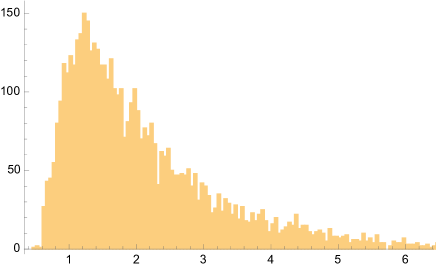
Figure 1: Illustration of Theorem 2.3 (a) by means of histograms of the $(1/K)^{\text{th}}$ variation $\sum_{k=0}^{b^{n}}|X((k+1)b^{-n})-X(kb^{-n})\big{|}^{1/K}$ for 5000 sample paths of the fractional Wiener–Weierstraß bridge with $n=16$, $b=2$, and parameters $H=0.7$ and $K=0.5$ (left) versus $H=0.5$ and $K=0.2$ (right).

Note that the increment process of the fractional Wiener–Weierstraß bridge is highly nonstationary. Therefore, classical results on the variation of Gaussian processes with stationary increments [23, 24] are not applicable.

Now we turn to the critical case $H=K$, which we discuss for $H=1/2$. In this case, the pattern observed in Theorem 2.3 breaks down and the quadratic variation of $X$ is infinite, even though the roughness exponent of $X$ is still equal to $1/2$.

Theorem 2.4.

Let $X$ be a Wiener–Weierstraß bridge with parameters $\alpha$, $b$, and $H=1/2$ where $\alpha^{2}b=1$ $($in particular, $H=1/2=K=1\wedge(-\log_{b}\alpha))$. Then the roughness exponent of $X$ is almost surely equal to $1/2$. Moreover, ${\mathbb{P}}$-a.s. for all $t\in(0,1]$,

$$\lim_{n\uparrow\infty}\frac{1}{n}\sum_{k=0}^{\lfloor tb^{n}\rfloor}\big{(}X((k+1)b^{-n})-X(kb^{-n})\big{)}^{2}=t.$$ (11)

In particular, the $p$-th variation of $X$ is almost surely infinite for $p\leq 2$ and zero for $p>2$.

Since the quadratic variation of the Wiener–Weierstraß bridge with $H=1/2=K$ is infinite, it cannot be a semimartingale. The following theorem extends the latter observation to all parameter choices.

Theorem 2.5.

For any $H\in(0,1)$, $\alpha\in(0,1)$, and $b\in\{2,3,\dots\}$, the fractional Wiener–Weierstraß bridge $X$ is not a semimartingale.

Let us discuss another aspect of Theorem 2.4. The convergence of the rescaled quadratic variations in (11) can be regarded as a Gladyshev-type theorem for the Wiener–Weierstraß bridge. As in the original work by Gladyshev [11], for the derivation of such results it is commonly assumed that the covariance function

$$c(s,t)\mathrel{\mathop{\ordinarycolon}}=\text{\rm cov}(X(s),X(t))$$

of the stochastic process $X$ satisfies certain differentiability conditions; see also [21]. However, the following result states that the covariance function of the fractional Wiener–Weierstraß bridge is often itself a fractal function; see Figure 2 for an illustration. For the particular case $H=1/2=K$ investigated in Theorem 2.4, the following result implies in particular that $t\mapsto c(1/2,t)$ is a nowhere differentiable Takagi–van der Waerden function. Thus, Theorem 2.4 might also be interesting as a case study for Gladyshev-type theorems without smoothness assumptions.

Proposition 2.6.

Suppose that $B$ is the standard fractional Brownian bridge with $\kappa$ given by (3) and that $K={-\log_{b}\alpha}<(2H)\wedge 1$. Then, for all $s\in(0,1)$, the covariance function $c(s,t)=\text{\rm cov}(X(s),X(t))$ is such that $t\mapsto c(s,t)$ has finite, nonzero, and linear $(1/K)^{\text{th}}$ variation. Moreover, if $b$ is even, $H=1/2$, and $s=1/2$, then the function $t\mapsto 2c(1/2,t)$ is the Takagi–van der Waerden function with parameters $b$ and $\alpha$, that is, the function in (1) for the tent map $\phi(t)=t\wedge(1-t)$.

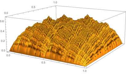
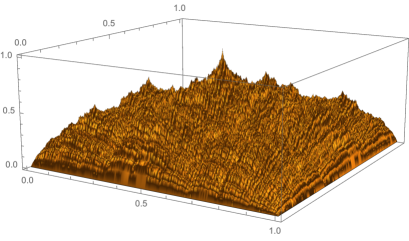
Figure 2: Covariance functions of the Wiener–Weierstraß bridge for $H=1/2$, $\alpha=1/2$, and $b=2$ (left) and $b=3$ (right).

A remarkable consequence of Theorem 2.3 and Proposition 2.6 is that for every $K\in(0,1)$ there is a Gaussian process whose sample paths and covariance function both admit the roughness exponent $K$. On the other hand, there exists no centered Gaussian process whose sample paths have a strictly lower roughness exponent than its covariance function. A precise statement of these facts is given in the following corollary.

Corollary 2.7.

Suppose that $p>1$ and $b\in\{2,3,\dots\}$.

1. There exists a centered Gaussian process $Y$ indexed by $[0,1]$ whose sample paths have ${\mathbb{P}}$-a.s. finite, nontrivial, and linear $p$-th variation and, for any $s\in(0,1)$, the covariance $t\mapsto c(s,t)\mathrel{\mathop{\ordinarycolon}}={\mathbb{E}}[Y(s)Y(t)]$ has finite, nontrivial, and linear $p$-th variation.

2. Suppose that $Y$ is any centered Gaussian process indexed by $[0,1]$ whose sample paths have ${\mathbb{P}}$-a.s. finite (though not necessarily nonzero) $p$-th variation. Then, for every $s\in[0,1]$,

   $$\limsup_{n\uparrow\infty}\sum_{k=0}^{b^{n}-1}\Big{|}c\big{(}s,(k+1)b^{-n}\big{)}-c\big{(}s,kb^{-n}\big{)}\Big{|}^{p}<\infty.$$ (12)

Remark 2.8.

We will see in Proposition A.1 that the sample paths of the fractional Wiener–Weierstraß bridge are ${\mathbb{P}}$-a.s. Hölder continuous with exponent $K$ for $K<H$. If $K\geq H$, then the trajectories are ${\mathbb{P}}$-a.s. Hölder continuous with exponent $\gamma$ for every $\gamma<H$.

Weierstraß bridges are not limited to fractional Brownian bridges. They can be defined and studied for a large class of underlying bridges. In the sequel, we are going to illustrate this by the Gaussian bridges arising from a continuous Gaussian martingale $M=(M(t))_{t\in[0,1]}$ with $M(0)=0$ and $\text{var}(M(1))={\mathbb{E}}[(M(1))^{2}]>0$. When letting

$$\kappa(t)\mathrel{\mathop{\ordinarycolon}}=\frac{\text{cov}(M(t),M(1))}{\text{var}(M(1))},$$

the law of the Gaussian bridge

$$B(t)=M(t)-\kappa(t)M(1),\qquad 0\leq t\leq 1,$$

is (at least informally) equal to the distribution of $M$ conditional on $\{M(1)=0\}$ (by [10], this holds for any continuous Gaussian process; (3) is an example). Since Gaussian martingales have deterministic quadratic variation, $\kappa$ can also be represented as follows,

$$\kappa(t)=\frac{\langle M\rangle_{t}}{\langle M\rangle_{1}}.$$

Now we take $\alpha\in(0,1)$ and $b\in\{2,3,\dots\}$ and let

$$X(t)\mathrel{\mathop{\ordinarycolon}}=\sum_{n=0}^{\infty}\alpha^{n}B(\{b^{n}t\}),\qquad 0\leq t\leq 1.$$ (13)

The process $X$ will be called the Gaussian Weierstraß bridge associated with $B$ and with parameters $\alpha$ and $b$.

Proposition 2.9.

Suppose that $\langle M\rangle_{t}=\int_{0}^{t}\varphi(s)\,ds$ for a bounded measurable function $\varphi\mathrel{\mathop{\ordinarycolon}}[0,1]\to[0,\infty)$ for which there exists a nonempty open interval $I\subset[0,1]$ such that $\varphi>0$ on $I$. Suppose moreover that $K={-\log_{b}\alpha}<1/2$. Then the corresponding Gaussian Weierstraß bridge (13) has finite, nonzero, and linear $(1/K)$-th variation along the $b$-adic partitions.

Outlook and some open questions.

Let us conclude this section by pointing out some interesting open questions and directions for future research that are beyond the scope of this paper.

1. Figure 1 suggests that the random variable $V$ in part (a) of Theorem 2.3 is a nondegenerate random variable with nonzero variance. Establishing this claim would provide a distinctive feature between the two regimes $H<K$ and $H>K$.

2. Theorem 2.4 analyzes only the case $H=1/2$, and it would be interesting to obtain a similar result for all $H\in(0,1)$. Based on the argument used to establish the convergence of expectation in Section 3.3, we expect that the following convergence holds for arbitrary $H\in(0,1)$ and ${\mathbb{P}}$-a.s. for all $t\in[0,1]$,

   $$\lim_{n\uparrow\infty}\frac{1}{n^{1/(2H)}}\sum_{k=0}^{\lfloor tb^{n}\rfloor}\big{|}X((k+1)b^{-n})-X(kb^{-n})\big{|}^{1/H}=\frac{2^{1/(2H)}\Gamma(\frac{H+1}{2H})}{\sqrt{\pi}}\cdot t.$$

3. Theorem 2.3 shows that the sample paths of $X$ have finite, nonzero, and linear $(H\wedge K)^{-1}$-th variation if $H\neq K$. Theorem 2.4, on the other hand, shows that this relation breaks down in the critical case $H=K$. A similar phenomenon appears already in the deterministic case (1) with Lipschitz continuous $\phi$. In this case, $H=1$ and we pick $\alpha=1/2$ and $b=2$ in (1), so that also $K=1$. Yet, the corresponding function (1) is typically not of bounded variation and, in the case where $\phi$ is the tent map, has been used as a classical example of a nowhere differentiable function [35]. It was shown in [14] that Weierstraß and Takagi–van der Waerden functions with critical roughness possess finite, nonzero, and linear $\Phi$-variation for the function $\Phi(x)=x(-\log x)^{-1/2}$, where $\Phi$-variation is understood in the Wiener–Young sense and taken along the $b$-adic partitions. We expect that a similar effect is in play for fractional Wiener–Weierstraß bridges and conjecture that for $H=K$ and $\Phi(x)=x^{1/H}(-\log x)^{-1/(2H)}$, ${\mathbb{P}}$-a.s. for all $t\in[0,1]$,

   $$\lim_{n\uparrow\infty}\sum_{k=0}^{\lfloor tb^{n}\rfloor}\Phi\big{(}\big{|}X((k+1)b^{-n})-X(kb^{-n})\big{|}\big{)}=\frac{2^{1/(2H)}\Gamma\big{(}\frac{H+1}{2H}\big{)}}{\sqrt{\pi}(-\log\alpha)^{1/(2H)}}\cdot t.$$

4. As pointed out by an anonymous referee, an interesting problem would be studying the fluctuations of the limits (10) and (11), as a function of $n$, the number of steps taken in the $b$-adic partition. For example, we may ask whether central limit theorems and large deviation principles can be established.

3 Proofs

Let $X$ denote the fractional Wiener–Weierstraß bridge with parameters $\alpha$, $b$, and $H$ and recall that the underlying fractional Brownian bridge is of the form $B(t)=W(t)-\kappa(t)W(1)$ for a fractional Brownian motion $W$ with Hurst parameter $H$ and a function $\kappa\mathrel{\mathop{\ordinarycolon}}[0,1]\to[0,1]$ that is Hölder continuous with exponent $\tau\in(H,1]$ and satisfies $\kappa(0)=0$ and $\kappa(1)=1$. Moreover, the parameters $K$ and $p$ are defined as

$$K=1\wedge(-\log_{b}\alpha)\quad\text{and}\quad p=\frac{1}{(K\wedge H)}.$$

Let us first discuss the $p$-th variation of a general function $f$ of the form (1). In (7), this $p$-th variation is defined as the limit of the terms

$$V_{n} \mathrel{\mathop{\ordinarycolon}}=\sum_{k=0}^{b^{n}-1}\big{|}f((k+1)b^{-n})-f(kb^{-n})\big{|}^{p}=\sum_{k=0}^{b^{n}-1}\bigg{|}\sum_{m=0}^{n-1}\alpha^{m}\Big{(}\phi(\{(k+1)b^{m-n}\})-\phi(\{kb^{m-n}\})\Big{)}\bigg{|}^{p}$$

$$=\alpha^{np}\sum_{k=0}^{b^{n}-1}\bigg{|}\sum_{m=1}^{n}\alpha^{-m}\Big{(}\phi(\{(k+1)b^{-m}\})-\phi(\{kb^{-m}\})\Big{)}\bigg{|}^{p},$$ (14)

where we have used the assumption $\phi(0)=\phi(1)$ in the second step. Following [32], we now let $(\Omega_{R},\mathscr{F}_{R},\mathbb{P}_{R})$ be a probability space supporting an independent sequence $U_{1},U_{2},\dots$ of random variables with a uniform distribution on $\{0,1,\dots,b-1\}$ and define the stochastic process

$$R_{m}\mathrel{\mathop{\ordinarycolon}}=\sum_{i=1}^{m}U_{i}b^{i-1},\qquad m\in\mathbb{N}.$$ (15)

The importance of the random variables $R_{m}$ and the need to have the random variables $R_{m}$ defined independently of our underlying Gaussian processes explain the subscript ‘$R$’ in our notation $(\Omega_{R},\mathscr{F}_{R},\mathbb{P}_{R})$. Note that each $R_{m}$ has a uniform distribution on $\{0,\dots,b^{m}-1\}$. Moreover, (15) ensures that

$$\{b^{-m}R_{n}\}=b^{-m}R_{m}\qquad\text{ for $m\leq n$.}$$ (16)

Following [32], we can now express the sum over $k$ in (14) through an expectation over $(R_{m})_{1\leq m\leq n}$ and then use (16) to obtain

$$V_{n} =(\alpha^{p}b)^{n}{\mathbb{E}}_{R}\bigg{[}\bigg{|}\sum_{m=1}^{n}\alpha^{-m}(\phi((R_{m}+1)b^{-m})-\phi(R_{m}b^{-m}))\bigg{|}^{p}\bigg{]}.$$ (17)

For notational clarity, the probability space on which the fractional Brownian motion $W$ and its corresponding bridge $B$ are defined will henceforth be denoted by $(\Omega_{W},\mathscr{F}_{W},\mathbb{P}_{W})$. The product space of these two probability spaces will be denoted by $(\Omega,\mathscr{F},\mathbb{P})$. That is, $\Omega=\Omega_{W}\times\Omega_{R}$, ${\mathscr{F}}={\mathscr{F}}_{W}\otimes{\mathscr{F}}_{R}$, and ${\mathbb{P}}={\mathbb{P}}_{W}\otimes{\mathbb{P}}_{R}$.

3.1 Proof of Theorem 2.3 (a)

In this section, we will deploy Proposition A.2 in Appendix A to prove part (a) of Theorem 2.3. Recall that this part addresses the situation in which $K<H$, which is equivalent to either $\alpha b^{H}>1$ or $\alpha^{p}b>1$.

Lemma 3.1.

In the context of Theorem 2.3 (a), let $(r_{m})_{m\in\mathbb{N}}$ be an arbitrary sequence of integers such that $r_{m}\in\{0,\dots,b^{m}-1\}$. Then the expectation

$${\mathbb{E}}_{W}\bigg{[}\bigg{(}\sum_{m=1}^{\infty}\alpha^{-m}\Big{(}B\Big{(}\frac{r_{m}+1}{b^{m}}\Big{)}-B\Big{(}\frac{r_{m}}{b^{m}}\Big{)}\Big{)}\bigg{)}^{2}\bigg{]}$$ (18)

is finite and strictly positive.

Proof.

For $m,n\in\mathbb{N}$, let us define $\Delta_{m}\kappa\mathrel{\mathop{\ordinarycolon}}=\kappa(\frac{r_{m}+1}{b^{m}})-\kappa(\frac{r_{m}}{b^{m}})$ and

$$f_{n}\mathrel{\mathop{\ordinarycolon}}=\sum_{m=1}^{n}\alpha^{-m}{\mathbbmss{1}}_{{}_{\scriptstyle[\frac{r_{m}}{b^{m}},\frac{r_{m}+1}{b^{m}}]}}(t)-\sum_{m=1}^{n}\alpha^{-m}\Delta_{m}\kappa.$$

Using $B(t)=W(t)-\kappa(t)W(1)$, we get

$$\sum_{m=1}^{n}\alpha^{-m}\Big{(}B\Big{(}\frac{r_{m}+1}{b^{m}}\Big{)}-B\Big{(}\frac{r_{m}}{b^{m}}\Big{)}\Big{)} =\sum_{m=1}^{n}\alpha^{-m}\Big{(}W\Big{(}\frac{r_{m}+1}{b^{m}}\Big{)}-W\Big{(}\frac{r_{m}}{b^{m}}\Big{)}\Big{)}-\sum_{m=1}^{n}\alpha^{-m}\Delta_{m}\kappa W(1)$$

$$=\int_{0}^{1}f_{n}(t)\,dW(t),$$ (19)

Here we have used the fact that the Wiener integral of the step function $f_{n}$ with respect to the fractional Brownian motion $W$ is given by the standard Riemann-type sum (see, e.g., p. 16 in [25]).

Since $\kappa$ is Hölder continuous with an exponent strictly larger than $H$, our assumption $\alpha b^{H}>1$ implies that the series $\sum_{m=1}^{\infty}\alpha^{-m}|\Delta_{m}\kappa|$ is finite. Moreover, for $k,\,n\in\mathbb{N}$ with $k<n$ and $p=1/H$,

$$\|f_{n}-f_{k}\|_{L^{p}[0,1]}\leq\sum_{m=k+1}^{n}\alpha^{-m}b^{-mH}+\sum_{m=k+1}^{n}\alpha^{-m}|\Delta_{m}\kappa|,$$ (20)

and the right-hand side can be made arbitrarily small by making $k$ large. Therefore, the sequence $(f_{n})$ converges in $L^{p}[0,1]$ to

$$f\mathrel{\mathop{\ordinarycolon}}=\sum_{m=1}^{\infty}\alpha^{-m}{\mathbbmss{1}}_{{}_{\scriptstyle[\frac{r_{m}}{b^{m}},\frac{r_{m}+1}{b^{m}}]}}-\sum_{m=1}^{\infty}\alpha^{-m}\Delta_{m}\kappa.$$ (21)

We claim next that there exists a nonempty open interval on which $f$ is nonzero. Indeed, we have

$$f(x)\geq\alpha^{-n}-\sum_{m=1}^{\infty}\alpha^{-m}|\Delta_{m}\kappa|\qquad\text{for }x\in\Big{[}\frac{r_{n}}{b^{n}},\frac{r_{n}+1}{b^{n}}\Big{]},$$ (22)

and when $n$ is sufficiently large, the right-hand side of the preceding inequality will be strictly positive.

Our next goal is to show that the Wiener integral $\int_{0}^{1}f(t)\,dW(t)$ exists and that

$$\sum_{m=1}^{n}\alpha^{-m}\Big{(}B\Big{(}\frac{r_{m}+1}{b^{m}}\Big{)}-B\Big{(}\frac{r_{m}}{b^{m}}\Big{)}\Big{)}=\int_{0}^{1}f_{n}(t)\,dW(t)\longrightarrow\int_{0}^{1}f(t)\,dW(t)\quad\text{in $L^{2}$.}$$ (23)

To this end, we will separately consider the cases $H=1/2$, $1/2<H<1$, and $0<H<1/2$.

First, we consider the case $H=1/2$. In this case, $W$ is a standard Brownian motion, and so (19), (21), and the standard Itô isometry yield our claim. In particular,

$${\mathbb{E}}_{W}\bigg{[}\bigg{(}\sum_{m=1}^{\infty}\alpha^{-m}\Big{(}B\Big{(}\frac{r_{m}+1}{b^{m}}\Big{)}-B\Big{(}\frac{r_{m}}{b^{m}}\Big{)}\Big{)}\bigg{)}^{2}\bigg{]}=\mathbb{E}_{W}\bigg{[}\bigg{(}\int_{0}^{1}f(t)\,dW(t)\bigg{)}^{2}\bigg{]}=\|f\|_{L^{2}[0,1]}^{2},$$ (24)

where the right-hand side is finite and strictly positive.

Next, we consider the case $1/2<H<1$. It follows from (21) in conjunction with Theorem 1.9.1 (ii) and Equation (1.6.3) in [25] that $\int_{0}^{1}f(t)\,dW(t)$ exists and (23) holds. In particular, the first identity in (24) holds also in our current case $1/2<H<1$, and another application of Theorem 1.9.1 (ii) in [25] yields that the expectation (18) is finite. To show that it is also strictly positive, we combine (23) and the fact that $f\in L^{p}[0,1]$ with Lemma 1.6.6, Theorem 1.9.1 (ii), and Equation (1.6.14) in [25] so as to obtain a constant $C>0$ such that

$${\mathbb{E}}_{W}\bigg{[}\bigg{(}\sum_{m=1}^{\infty}\alpha^{-m}\Big{(}B\Big{(}\frac{r_{m}+1}{b^{m}}\Big{)}-B\Big{(}\frac{r_{m}}{b^{m}}\Big{)}\Big{)}\bigg{)}^{2}\bigg{]} =C\int_{0}^{1}\int_{0}^{1}f(u)f(v)|u-v|^{2H-2}\,du\,dv.$$ (25)

Since $H<1$, the function $t\mapsto t^{2H-2}$ is strictly convex and decreasing on $(0,\infty)$. The integral kernel $K(u,v)\mathrel{\mathop{\ordinarycolon}}=|u-v|^{2H-2}$ is hence strictly positive definite; see Proposition 2 in [2]. Since we have already seen that $f(t)$ is nonzero on a nonempty open interval, the integral on the right-hand side of (25) must hence be strictly positive.

Finally, we consider the case $0<H<1/2$. Recall from Section 1.6 in [25] that there exists an unbounded linear integral operator $M_{-}^{H}$ from $L^{1}[0,1]$ to $L^{2}(\mathbb{R})$ such that

$$\mathbb{E}\bigg{[}\bigg{(}\int_{0}^{1}g(t)\,dW(t)\bigg{)}^{2}\bigg{]}=\|M_{-}^{H}g\|^{2}_{L^{2}(\mathbb{R})}$$ (26)

for all $g$ in the domain of $M_{-}^{H}$, which is denoted by $L^{2}_{H}[0,1]$. The specific form of $M_{-}^{H}$ will not be needed here. All we will need is that there exists a universal constant $C_{H}>0$ such that

$$\big{|}\widehat{M_{-}^{H}g}(x)\big{|}=C_{H}|\widehat{g}(x)|\cdot|x|^{\frac{1}{2}-H},\qquad x\in\mathbb{R},$$

where $\widehat{g}(x)=\int e^{ixt}g(t)\,dt$ denotes the Fourier transform of $g$; see Theorem 1.1.5 and (1.3.3) in [25]. By Parseval’s identity, we hence have

$$\|M_{-}^{H}g\|_{L^{2}(\mathbb{R})}^{2}=C_{H}^{2}\int|\widehat{g}(x)|^{2}\cdot|x|^{1-2H}\,dx,\qquad g\in L^{2}_{H}[0,1].$$ (27)

Note that

$$\big{|}\widehat{{\mathbbmss{1}}_{{}_{\scriptstyle[\frac{r_{m}}{b^{m}},\frac{r_{m}+1}{b^{m}}]}}}(x)\big{|}=\Big{|}\frac{e^{ix(r_{m}+1)/b^{m}}-e^{ixr_{m}/b^{m}}}{x}\Big{|}\leq\begin{cases}b^{-m}&\text{if $|x|\leq b^{m}$,}\\ 2/|x|&\text{otherwise.}\end{cases}$$

Therefore, for $n<N$ and $c\mathrel{\mathop{\ordinarycolon}}=\|M^{H}_{-}{\mathbbmss{1}}_{{}_{\scriptstyle[0,1]}}\|_{L^{2}(\mathbb{R})}/C_{H}$,

$$\frac{1}{C_{H}}\big{\|}M^{H}_{-}f_{N}-M^{H}_{-}f_{n}\big{\|}_{L^{2}(\mathbb{R})}$$

$$\leq\frac{1}{C_{H}}\sum_{m=n+1}^{N}\alpha^{-m}\big{\|}M^{H}_{-}{\mathbbmss{1}}_{{}_{\scriptstyle[\frac{r_{m}}{b^{m}},\frac{r_{m}+1}{b^{m}}]}}\big{\|}_{L^{2}(\mathbb{R})}+c\sum_{m=n+1}^{N}\alpha^{-m}|\Delta_{m}\kappa|$$

$$\leq\sum_{m=n+1}^{N}\alpha^{-m}b^{-m}\sqrt{2\int_{0}^{b^{m}}x^{1-2H}\,dx}+\sum_{m=n+1}^{N}\alpha^{-m}\sqrt{8\int_{b^{m}}^{\infty}x^{-1-2H}\,dx}+c\sum_{m=n+1}^{N}\alpha^{-m}|\Delta_{m}\kappa|$$

$$=\frac{1}{\sqrt{1-H}}\sum_{m=n+1}^{N}\alpha^{-m}b^{-mH}+\sqrt{\frac{4}{H}}\sum_{m=n+1}^{N}\alpha^{-m}b^{-mH}+c\sum_{m=n+1}^{N}\alpha^{-m}|\Delta_{m}\kappa|.$$

Since $\alpha b^{H}>1$, the latter expression is less than any given $\varepsilon>0$ as soon as $n$ is sufficiently large. By Remark 1.6.3 in [25], the space $L^{2}_{H}[0,1]$ is complete with respect to the norm $\|f\|_{L^{2}_{H}[0,1]}=\|M_{-}^{H}f\|_{L^{2}(\mathbb{R})}$ if $0<H<1/2$, and so we must have $f_{n}\to f$ in $L^{2}_{H}[0,1]$. Thus, the Wiener integral of $f$ exists and we also have (23), which gives

$$\int_{0}^{1}f(t)\,dW(t)=\sum_{m=1}^{\infty}\alpha^{-m}\Big{(}B\Big{(}\frac{r_{m}+1}{b^{m}}\Big{)}-B\Big{(}\frac{r_{m}}{b^{m}}\Big{)}\Big{)}.$$ (28)

By (26), the $L^{2}$-norm of this Wiener integral is given by $\|M_{-}^{H}f\|_{L^{2}(\mathbb{R})}$, and (27) yields that $\|M_{-}^{H}f\|_{L^{2}(\mathbb{R})}$ is finite and also strictly positive, since $f$ is nonzero on a nonempty open interval. ∎

Proof of Theorem 2.3 (a).

To apply Proposition A.2 in Appendix A, choose $\gamma\in(K,H)$ so that $\alpha b^{\gamma}>1$ and pick a version of $B$ with $\gamma$-Hölder continuous sample paths. Lemma 3.1 yields that

$$0<{\mathbb{E}}_{W}\bigg{[}\bigg{(}\sum_{m=1}^{\infty}\alpha^{-m}\Big{(}B\Big{(}\frac{R_{m}+1}{b^{m}}\Big{)}-B\Big{(}\frac{R_{m}}{b^{m}}\Big{)}\Big{)}\bigg{)}^{2}\bigg{]}<\infty\quad\text{$\mathbb{P}_{R}$-a.s.}$$

The argument of the expectation is normally distributed, and so

$$\mathbb{P}_{W}\bigg{(}\sum_{m=1}^{\infty}\alpha^{-m}\Big{(}B\Big{(}\frac{R_{m}+1}{b^{m}}\Big{)}-B\Big{(}\frac{R_{m}}{b^{m}}\Big{)}\Big{)}=0\,\bigg{)}=0\quad\text{$\mathbb{P}_{R}$-a.s.}$$

Hence we conclude that

$$\mathbb{P}\bigg{(}\sum_{m=1}^{\infty}\alpha^{-m}\Big{(}B\Big{(}\frac{R_{m}+1}{b^{m}}\Big{)}-B\Big{(}\frac{R_{m}}{b^{m}}\Big{)}\Big{)}=0\bigg{)}=0.$$

Therefore, Proposition A.2 yields the result. ∎

Remark 3.2.

It follows from Proposition A.2 that the $p$-th variation of $X$ is ${\mathbb{P}}_{W}$-a.s. given by

$$\langle X\rangle^{(p)}_{1}={\mathbb{E}}_{R}\bigg{[}\bigg{|}\sum_{m=1}^{\infty}\alpha^{-m}\Big{(}B\Big{(}\frac{R_{m}+1}{b^{m}}\Big{)}-B\Big{(}\frac{R_{m}}{b^{m}}\Big{)}\Big{)}\bigg{|}^{p}\bigg{]}.$$ (29)

Furthermore, for each realization of the random variables $(R_{m})$, the identity (28) shows that the expression

$$\sum_{m=1}^{\infty}\alpha^{-m}\Big{(}B\Big{(}\frac{R_{m}+1}{b^{m}}\Big{)}-B\Big{(}\frac{R_{m}}{b^{m}}\Big{)}\Big{)}$$

is equal to a Wiener integral with respect to the fractional Brownian motion $W$. Thus, the right-hand side of (29) can be regarded as a mixture of the $p$-th powers of certain Wiener integrals.

3.2 Proof of Theorem 2.3 (b)

In this section, we will prove part (b) of Theorem 2.3. Recall that this part addresses the situation in which $K>H$, which is equivalent to either $\alpha b^{H}<1$ or $\alpha^{p}b<1$. Let us introduce the notation

$$V_{n}\mathrel{\mathop{\ordinarycolon}}=\sum_{k=0}^{b^{n}-1}|X((k+1)b^{-n})-X(kb^{-n})|^{p}.$$ (30)

Recall also the three probability spaces $(\Omega_{R},\mathscr{F}_{R},\mathbb{P}_{R})$, $(\Omega_{W},\mathscr{F}_{W},\mathbb{P}_{W})$, and $(\Omega,\mathscr{F},\mathbb{P})=(\Omega_{W}\times\Omega_{R},{\mathscr{F}}_{W}\otimes{\mathscr{F}}_{R},{\mathbb{P}}_{W}\otimes{\mathbb{P}}_{R})$ introduced above. Sections 3.2.1 and 3.2.2 are devoted to the proof of Theorem 2.3 (b) when $t=1$, and we extend the arguments for a general $t\in[0,1]$ in Section 3.2.3.

3.2.1 Convergence of the expectation

In this first part of the proof, we will prove that the expected $p$-th variation, ${\mathbb{E}}_{W}[V_{n}]$, converges to $c_{H}/(1-\alpha^{2}b^{2H})^{p/2}$, where

$$c_{H}\mathrel{\mathop{\ordinarycolon}}=\frac{2^{1/(2H)}\Gamma(\frac{H+1}{2H})}{\sqrt{\pi}}.$$

Here and later, we denote by ${\mathbbm{1}}_{A}$ the indicator function of a set $A$.

Lemma 3.3.

The expected $p$-th variation is of the form

$${\mathbb{E}}_{W}[V_{n}]=(\alpha^{p}b)^{n}{\mathbb{E}}\bigg{[}\bigg{|}\int_{0}^{1}f_{n}(x)\,dW(x)\bigg{|}^{p}\bigg{]},$$

where ${\mathbb{E}}[\,\cdot\,]$ denotes the expectation with respect to ${\mathbb{P}}={\mathbb{P}}_{W}\otimes{\mathbb{P}}_{R}$ and $f_{n}(x)=g_{n}(x)-h_{n}$ for

$$g_{n}(x)\mathrel{\mathop{\ordinarycolon}}=\sum_{m=1}^{n}\alpha^{-m}{\mathbbm{1}}_{[R_{m}b^{-m},(R_{m}+1)b^{-m}]}(x)\quad\text{and}\quad h_{n}\mathrel{\mathop{\ordinarycolon}}=\sum_{m=1}^{n}\alpha^{-m}(\kappa((R_{m}+1)b^{-m})-\kappa(R_{m}b^{-m})).$$

Proof.

By (17) and (2),

$${\mathbb{E}}[V_{n}] =(\alpha^{p}b)^{n}{\mathbb{E}}_{W}\bigg{[}{\mathbb{E}}_{R}\bigg{[}\bigg{|}\sum_{m=1}^{n}\alpha^{-m}\bigg{(}B((R_{m}+1)b^{-m})-B(R_{m}b^{-m})\bigg{)}\bigg{|}^{p}\bigg{]}\bigg{]}$$

$$=(\alpha^{p}b)^{n}{\mathbb{E}}_{R}\bigg{[}{\mathbb{E}}_{W}\bigg{[}\bigg{|}\int_{0}^{1}f_{n}(x)\,dW(x)\bigg{|}^{p}\bigg{]}\bigg{]},$$

where we have used the fact that the Wiener integral of the step function $f_{n}$ is given by the standard Riemann-type sum (see, e.g., p. 16 in [25]). ∎

We will eventually prove that

$${\mathbb{E}}\bigg{[}\bigg{|}\int_{0}^{1}f_{n}(x)\,dW(x)\bigg{|}^{p}\bigg{]}$$

is of order $(\alpha^{p}b)^{-n}$ and the contribution from the time-independent constants $h_{n}$ are asymptotically negligible. This argument will become valid after having shown that the contribution from the functions $g_{n}$ gives the correct magnitude. This is our current focus. We start with the following elementary lemma.

Lemma 3.4.

For given $\gamma\in(0,1)$, $C>0$, and $0<a<\beta$, suppose that we have constants $C_{n}=(1+o(1))C\beta^{n}$ and random variables $\eta_{n}$ for which ${\mathbb{E}}[|\eta_{n}|]=O(a^{n})$. Then ${\mathbb{E}}[|C_{n}+\eta_{n}|^{\gamma}]=(1+o(1))C^{\gamma}\beta^{n\gamma}$.

Proof.

We have

$${\mathbb{E}}\bigg{[}\bigg{|}1+\frac{\eta_{n}}{C_{n}}\bigg{|}^{\gamma}\bigg{]} =\int_{0}^{\infty}{\mathbb{P}}\bigg{(}\bigg{|}1+\frac{\eta_{n}}{C_{n}}\bigg{|}^{\gamma}>x\bigg{)}\,dx$$

$$=\int_{0}^{\infty}{\mathbb{P}}\bigg{(}\frac{\eta_{n}}{C_{n}}>x^{1/\gamma}-1\bigg{)}\,dx+\int_{0}^{\infty}{\mathbb{P}}\bigg{(}\frac{\eta_{n}}{C_{n}}<-x^{1/\gamma}-1\bigg{)}\,dx.$$ (31)

We show that the first integral converges to one. First, we have for any $\varepsilon>0$,

$$1\geq\int_{0}^{1}{\mathbb{P}}\bigg{(}\frac{\eta_{n}}{C_{n}}>x^{1/\gamma}-1\bigg{)}\,dx\geq\int_{0}^{1-\varepsilon}{\mathbb{P}}\big{(}|\eta_{n}|<(1-(1-\varepsilon)^{1/\gamma})C_{n}\big{)}\,dx\longrightarrow 1-\varepsilon.$$

To deal with the remaining part of the integral, we let $L$ denote a constant for which ${\mathbb{E}}[|\eta_{n}|]/C_{n}\leq La^{n}/\beta^{n}$. Then, by Markov’s inequality for $y>0$,

$${\mathbb{P}}(|\eta_{n}|>yC_{n})\leq\frac{{\mathbb{E}}[|\eta_{n}|]}{yC_{n}}\leq L\frac{a^{n}}{y\beta^{n}}.$$

Therefore,

$$0\leq\int_{1}^{\infty}{\mathbb{P}}\bigg{(}\frac{\eta_{n}}{C_{n}}>x^{1/\gamma}-1\bigg{)}\,dx\leq\varepsilon+L\frac{a^{n}}{\beta^{n}}\int_{1+\varepsilon}^{\infty}\frac{1}{x^{1/\gamma}-1}\,dx\longrightarrow\varepsilon.$$

The second integral in (31) converges to zero by a similar argument. This completes the proof. ∎

In the following, we will frequently deal with sums of covariances, for which the following easy observation will be useful.

Lemma 3.5.

Let $m,k\in\mathbb{N},m>k$. Let $S=\{0,1,\dots,b^{m}-1\}$ and fix $j\in\{1-b^{m},\dots,0,\dots,b^{m}-1\}$. Then $\#\{i\in S\mathrel{\mathop{\ordinarycolon}}b^{m}\{ib^{-k}\}-i=j\}\leq 1$.

Proof.

Note that $b^{m}\{ib^{-k}\}=(ib^{m-k})\!\!\mod b^{m}$, where $n\!\!\mod{b^{m}}$ is the remainder of $n$ divided by $b^{m}$. Suppose $i_{1},i_{2}\in S$ are such that $(i_{1}b^{m-k})\!\!\mod{b^{m}}-i_{1}=(i_{2}b^{m-k})\!\!\mod{b^{m}}-i_{2}$. Then $b^{m}$ divides $(i_{1}-i_{2})(b^{m-k}-1)$ and $b^{m}$ divides $(i_{1}-i_{2})$, implying $i_{1}=i_{2}$. ∎

From now on, $L>0$ will denote a generic constant that may depend only on $\alpha,b,H,\kappa$ but not on anything else (in particular, not on $n,m,k$). The value of $L$ may change at each occurrence.

Proposition 3.6.

For $g_{n}$ as in Lemma 3.3, we have

$$(\alpha^{p}b)^{n}{\mathbb{E}}\bigg{[}\bigg{|}\int_{0}^{1}g_{n}(x)\,dW(x)\bigg{|}^{p}\bigg{]}=\frac{(1+o(1))c_{H}}{(1-\alpha^{2}b^{2H})^{p/2}}.$$

Proof.

If $Y$ is any centered Gaussian random variable, then ${\mathbb{E}}[|Y|^{p}]={\mathbb{E}}[Y^{2}]^{p/2}{\mathbb{E}}[|Z|^{p}]$, where $Z$ is standard normally distributed. Since, moreover, ${\mathbb{E}}[|Z|^{p}]=c_{H}$, we have

$${\mathbb{E}}\bigg{[}\bigg{|}\int_{0}^{1}g_{n}(x)\,dW(x)\bigg{|}^{p}\bigg{]}=c_{H}{\mathbb{E}}_{R}\bigg{[}\bigg{(}{\mathbb{E}}_{W}\bigg{[}\bigg{(}\int_{0}^{1}g_{n}(x)\,dW(x)\bigg{)}^{2}\bigg{]}\bigg{)}^{p/2}\bigg{]}.$$ (32)

To deal with the ${\mathscr{F}}_{R}$-measurable random variable ${\mathbb{E}}_{W}[(\int_{0}^{1}g_{n}(x)\,dW(x))^{2}]$, we define

$$\xi_{k,m} \mathrel{\mathop{\ordinarycolon}}={\mathbb{E}}_{W}\Big{[}\big{(}W((R_{k}+1)b^{-k})-W(R_{k}b^{-k})\big{)}\big{(}W((R_{m}+1)b^{-m})-W(R_{m}b^{-m})\big{)}\Big{]}.$$

With this notation, the definition of $g_{n}$ gives

$${\mathbb{E}}_{W}\bigg{[}\bigg{(}\int_{0}^{1}g_{n}(x)\,dW(x)\bigg{)}^{2}\bigg{]}=\sum_{m=1}^{n}\sum_{k=1}^{n}\alpha^{-m-k}\xi_{k,m}.$$ (33)

Note that the diagonal terms $\xi_{m,m}$ are deterministic and given by $b^{-2mH}$. Hence,

$$C_{n}\mathrel{\mathop{\ordinarycolon}}=\sum_{m=1}^{n}\xi_{m,m}=\sum_{m=1}^{n}\alpha^{-2m}b^{-2mH}=\frac{(\alpha^{2}b^{2H})^{-n}-1}{1-\alpha^{2}b^{2H}}=(1+o(1))\frac{(\alpha b^{H})^{-2n}}{1-\alpha^{2}b^{2H}}.$$ (34)

When denoting the sum of all off-diagonal terms by

$$\eta_{n}\mathrel{\mathop{\ordinarycolon}}=2\sum_{1\leq k<m\leq n}\alpha^{-m-k}\xi_{k,m},$$

we get that

$${\mathbb{E}}\bigg{[}\bigg{|}\int_{0}^{1}g_{n}(x)\,dW(x)\bigg{|}^{p}\bigg{]}=c_{H}{\mathbb{E}}_{R}\big{[}\big{|}C_{n}+\eta_{n}\big{|}^{p/2}\big{]}.$$ (35)

For dealing with the right-hand expectation, we need to distinguish between the cases $H\geq 1/2$ and $H<1/2$.

For $H\geq 1/2$, the increments of fractional Brownian motion are nonnegatively correlated, so each $\xi_{k,m}$ is nonnegative, and so is $\eta_{n}$. To apply Lemma 3.4, we aim to bound ${\mathbb{E}}[\xi_{n}]={\mathbb{E}}[|\xi_{n}|]$ from above. Due to the stationarity of increments of $W$, the random variable $\xi_{k,m}$ depends only on $R_{k}b^{-k}-R_{m}b^{-m}$. Note that since $k<m$, we have $R_{k}b^{-k}=\{R_{m}b^{-k}\}$. So using the fact that $R_{m}$ is uniformly distributed on $\{0,1,\dots,b^{m}-1\}$ and applying Lemma 3.5 and a telescoping argument yields

$${\mathbb{E}}_{R}[\xi_{k,m}] =b^{-m}\sum_{i=0}^{b^{m}-1}{\mathbb{E}}_{W}\big{[}(W(\{ib^{-k}\}+b^{-k})-W(\{ib^{-k}\}))(W((i+1)b^{-m})-W(ib^{-m}))\big{]}$$

$$=b^{-m}\sum_{i=0}^{b^{m}-1}{\mathbb{E}}_{W}\big{[}W(b^{-k})(W((i+1)b^{-m}-\{ib^{-k}\})-W(ib^{-m}-\{ib^{-k}\}))\big{]}$$

$$\leq b^{-m}\sum_{j=-b^{m}}^{b^{m}-1}{\mathbb{E}}_{W}\big{[}W(b^{-k})(W((j+1)b^{-m})-W(jb^{-m}))\big{]}$$ (36)

$$=b^{-m}{\mathbb{E}}_{W}\big{[}W(b^{-k})(W(1)-W(-1))\big{]}=b^{-m}((1+b^{-k})^{2H}-(1-b^{-k})^{2H})$$

$$\leq Lb^{-m-k},$$

where the last step follows from the mean-value theorem. Combining the above yields

$${\mathbb{E}}_{R}[|\eta_{n}|]={\mathbb{E}}_{R}[\eta_{n}]=2\sum_{1\leq k<m\leq n}\alpha^{-m-k}{\mathbb{E}}_{R}[\xi_{k,m}]\leq L\sum_{1\leq k<m\leq n}\alpha^{-m-k}b^{-m-k}=O(a^{n}),$$ (37)

where $a=(\alpha b)^{-2}$ for $\alpha b<1$, and $a$ is an arbitrary number in $(1,(\alpha b^{H})^{-2})$ for $\alpha b\geq 1$. Since $a<(\alpha^{2}b^{2H})^{-1}=\mathrel{\mathop{\ordinarycolon}}\beta$, it follows from Lemma 3.4 with $C=(1-\alpha^{2}b^{2H})^{-1}$, and $\gamma=p/2$ that ${\mathbb{E}}[|C_{n}+\eta_{n}|^{p/2}]=(1+o(1))C^{p/2}(\alpha^{p}b)^{-n}$. In view of (35), this completes the proof for $1/2\leq H<1$.

We now turn to the case $0<H<1/2$, for which $p/2\geq 1$. We will prove below that for $k<m$,

$$\|\xi_{m,k}\|_{L^{p/2}({\mathbb{P}}_{R})}\leq L(b^{-m}+b^{-4Hm}).$$ (38)

Then Minkowski’s inequality and $0<H<1/2$ yields that

$$\|\eta_{n}\|_{L^{p/2}({\mathbb{P}}_{R})} \leq 2\sum_{1\leq k<m\leq n}\alpha^{-m-k}\|\xi_{k,m}\|_{L^{p/2}({\mathbb{P}}_{R})}\leq L\sum_{1\leq k<m\leq n}\alpha^{-m-k}(b^{-m}+b^{-4Hm})=o((\alpha^{2}b^{2H})^{-n}).$$

Thus, by (35) and another application of Minkowski’s inequality,

$${\mathbb{E}}\bigg{[}\bigg{|}\int_{0}^{1}g_{n}(x)\,dW(x)\bigg{|}^{p}\bigg{]}^{2/p} =c_{H}^{2/p}\big{(}C_{n}+O(\|\eta_{n}\|_{L^{p/2}({\mathbb{P}}_{R})})\big{)}=c_{H}^{2/p}C_{n}+o((\alpha^{2}b^{2H})^{-n}).$$

Multiplying the preceding identity with $(\alpha^{p}b)^{2n/p}=(\alpha^{2}b^{2H})^{n}$ and using (34) will then yield the assertion for $0<H<1/2$.

It remains to establish (38). By arguing as in (36), we write

$${\mathbb{E}}_{R}\big{[}|\xi_{m,k}|^{p/2}\big{]}$$

$$\leq b^{-m}\sum_{j=-b^{m}}^{b^{m}-1}\big{|}{\mathbb{E}}_{W}\big{[}W(b^{-k})(W((j+1)b^{-m})-W(jb^{-m}))\big{]}\big{|}^{p/2}$$

$$=b^{-m}\sum_{j=-b^{m}}^{b^{m}-1}\left|\big{|}(j+1)b^{-m}\big{|}^{2H}+\big{|}jb^{-m}-b^{-k}\big{|}^{2H}-\big{|}jb^{-m}\big{|}^{2H}-\big{|}(j+1)b^{-m}-b^{-k}\big{|}^{2H}\right|^{p/2}$$

$$\leq Lb^{-m}\sum_{j=-b^{m}}^{b^{m}-1}\left(\left|\big{|}(j+1)b^{-m}\big{|}^{2H}-\big{|}jb^{-m}\big{|}^{2H}\right|^{p/2}+\left|\big{|}jb^{-m}-b^{-k}\big{|}^{2H}-\big{|}(j+1)b^{-m}-b^{-k}\big{|}^{2H}\right|^{p/2}\right)$$

$$\leq Lb^{-m}\sum_{j=0}^{2b^{m}-1}\left(\big{(}(j+1)b^{-m}\big{)}^{2H}-\big{(}jb^{-m}\big{)}^{2H}\right)^{p/2}$$

$$\leq Lb^{-2m}+Lb^{-m}\sum_{j=2}^{2b^{m}-1}\left(\big{(}(j+1)b^{-m}\big{)}^{2H}-\big{(}jb^{-m}\big{)}^{2H}\right)^{p/2}.$$

By the mean-value theorem, for $j\geq 1$,

$$\big{(}(j+1)b^{-m}\big{)}^{2H}-\big{(}jb^{-m}\big{)}^{2H}\leq L\big{(}jb^{-m}\big{)}^{2H-1}b^{-m}=Lj^{2H-1}b^{-2mH}.$$

Therefore, since $p>2$,

$$b^{-m}\sum_{j=2}^{2b^{m}-1}\left(\big{(}(j+1)b^{-m}\big{)}^{2H}-\big{(}jb^{-m}\big{)}^{2H}\right)^{p/2}\leq Lb^{-2m}\sum_{j=2}^{2b^{m}-1}j^{1-p/2}\leq Lb^{-pm/2}.$$

Combining the above we obtain $\|\xi_{m,k}\|_{L^{p/2}({\mathbb{P}}_{R})}\leq L(b^{-2m}+b^{-pm/2})^{2/p}\leq L(b^{-4Hm}+b^{-m})$ and thus (38). ∎

Proposition 3.7.

Proposition 3.6 holds with $g_{n}$ replaced by $f_{n}$, i.e.,

$$(\alpha^{p}b)^{n}{\mathbb{E}}\bigg{[}\bigg{|}\int_{0}^{1}f_{n}(x)\,dW(x)\bigg{|}^{p}\bigg{]}=\frac{(1+o(1))c_{H}}{(1-\alpha^{2}b^{2H})^{p/2}}.$$

Proof.

Recall from Lemma 3.3 that $f_{n}=g_{n}-h_{n}$ where $h_{n}=\sum_{m=1}^{n}\alpha^{-m}(\kappa((R_{m}+1)b^{-m})-\kappa(R_{m}b^{-m}))$. By (32), Minkowski’s inequality and the $\tau$-Hölder continuity of $\kappa$,

$$\bigg{\|}\int_{0}^{1}h_{n}\,dW(x)\bigg{\|}_{L^{p}({\mathbb{P}})} =\Big{(}{\mathbb{E}}_{R}\big{[}|h_{n}|^{p}\cdot{\mathbb{E}}_{W}[|W(1)|^{p}]\big{]}\Big{)}^{1/p}$$

$$=c_{H}^{1/p}\left\lVert\sum_{m=1}^{n}\alpha^{-m}(\kappa((R_{m}+1)b^{-m})-\kappa(R_{m}b^{-m}))\right\rVert_{L^{p}({\mathbb{P}}_{R})}$$

$$\leq c_{H}^{1/p}\sum_{m=1}^{n}\alpha^{-m}\left\lVert(\kappa((R_{m}+1)b^{-m})-\kappa(R_{m}b^{-m}))\right\rVert_{L^{p}({\mathbb{P}}_{R})}$$

$$\leq L\sum_{m=1}^{n}\alpha^{-m}b^{-m\tau}=o((\alpha b^{H})^{-n}).$$

Thus the assertion follows by applying Minkowski’s inequality to $\|\int f_{n}\,dW\|_{L^{p}({\mathbb{P}})}=\|\int(g_{n}-h_{n})\,dW\|_{L^{p}({\mathbb{P}})}$ and using Proposition 3.6. ∎

3.2.2 A concentration bound

Having proved the convergence of the expected $p$-th variation, we now turn to the second part of the proof, which establishes a concentration inequality and thus ${\mathbb{P}}_{W}$-a.s. convergence. Recall the notation $V_{n}$ from (30). We also introduce the shorthand notation

$$t^{(n)}_{i}=ib^{-n},\qquad\text{$n\in\mathbb{N}$ and $i=0,\dots,b^{n}$,}$$

and we will simply write $t_{i}$ in place of $t_{i}^{(n)}$ if the value of $n$ is clear from the context. The following lemma can be proved analogously as Lemma 10.2.2 in [24]; all one needs is to replace [24, Equation (5.152)] with the Borell–TIS inequality in the form of Theorem 2.1.1 in [1].

Lemma 3.8.

Let $q>1$ with $p^{-1}+q^{-1}=1$ and define

$$M_{n}\mathrel{\mathop{\ordinarycolon}}=\bigg{\{}(\mu_{1},\dots,\mu_{b^{n}})\in{\mathbb{R}}^{b^{n}}\mathrel{\mathop{\ordinarycolon}}\sum_{j=1}^{b^{n}}|\mu_{j}|^{q}\leq 1\bigg{\}}$$

and

$$\sigma_{n}^{2}\mathrel{\mathop{\ordinarycolon}}=\sup_{(\mu_{k})\in M_{n}}\sum_{i=1}^{b^{n}}\sum_{j=1}^{b^{n}}\mu_{i}\mu_{j}{\mathbb{E}}[(X(t_{i})-X(t_{i-1}))(X(t_{j})-X(t_{j-1}))].$$ (39)

Then

$${\mathbb{P}}\left(|V_{n}^{H}-{\mathbb{E}}[V_{n}^{H}]|>s\right)\leq 2e^{-\frac{s^{2}}{2\sigma_{n}^{2}}}.$$ (40)

The preceding lemma will be needed in the proof of the following proposition. In the sequel, $\lambda$ will denote a generic constant in $(0,1)$ that may depend only on $\alpha,b,H$ and that may differ from occurrence to occurrence.

Proposition 3.9.

Suppose that (40) holds and $\sigma_{n}=O(\lambda^{n})$ for some $\lambda\in(0,1)$. Then $V_{n}$ converges almost surely to

$$C_{p}\mathrel{\mathop{\ordinarycolon}}=\frac{c_{H}}{(1-\alpha^{2}b^{2/p})^{p/2}}=\frac{c_{H}}{(1-\alpha^{2}b^{2H})^{1/(2H)}}.$$

That is, Theorem 2.3 holds for $t=1$.

Proof.

Combining Proposition 3.7 and Lemma 3.3 yields $\lim_{n}{\mathbb{E}}[V_{n}]=C_{p}$. We also claim that the sequence $(V_{n})_{n\in\mathbb{N}}$ is uniformly integrable. To see why, choose $n_{0}\in\mathbb{N}$ such that ${\mathbb{E}}[V_{n}]\leq C_{p}+1$ and $\sigma_{n}\leq\sqrt{2\pi}$ for all $n\geq n_{0}$. Then, for $n\geq n_{0}$ and $c>(C_{p}+2)^{p}$,

$${\mathbb{E}}[V_{n}{\mathbbmss{1}}_{{}_{\scriptstyle\{V_{n}>c\}}}] =\int_{c}^{\infty}{\mathbb{P}}(V_{n}>r)\,dr=p\int_{c^{1/p}-C_{p}-2}{\mathbb{P}}(V_{n}>(C_{p}+2+s)^{p})(C_{p}+2+s)^{p-1}\,ds$$

$$\leq p\int_{c^{1/p}-C_{p}-2}^{\infty}{\mathbb{P}}\left(|V_{n}^{H}-{\mathbb{E}}[V_{n}^{H}]|>s+\frac{\sigma_{n}}{\sqrt{2\pi}}\right)(C_{p}+2+s)^{p-1}\,ds$$

$$\leq 2p\int_{c^{1/p}-C_{p}-2}^{\infty}e^{-s^{2}/4\pi}(C_{p}+2+s)^{p-1}\,ds,$$

where we have used (40) in the final step. Clearly, the latter integral can be made arbitrarily small by increasing $c$, which proves the claimed uniform integrability.

Next, since ${\mathbb{E}}[V_{n}^{H}]\leq{\mathbb{E}}[V_{n}]^{H}$, the sequence $({\mathbb{E}}[V_{n}^{H}])_{n\in\mathbb{N}}$ is bounded. Suppose there is a subsequence $(n_{k})$ such that ${\mathbb{E}}[V_{n_{k}}^{H}]$ converges to the finite limit $\ell$ as $k\uparrow\infty$. Then (40) with the choice $s_{n}=n\sigma_{n}$ and the Borel–Cantelli lemma give $V_{n_{k}}^{H}\to\ell$ ${\mathbb{P}}$-a.s. and in turn $V_{n_{k}}\to\ell^{p}$ ${\mathbb{P}}$-a.s. Due to the established uniform integrability, the latter convergence also holds in $L^{1}$, and we obtain $\ell^{p}=C_{p}$. It follows that $\ell$ is the unique accumulation point of the sequence $({\mathbb{E}}[V^{H}_{n}])_{n\in\mathbb{N}}$ and equal to $C_{p}^{1/p}$. Therefore, we can replace the above subsequence $(n_{k})$ by $\mathbb{N}$, so that $V_{n}\to C_{p}$ ${\mathbb{P}}$-a.s. as required. ∎

In the remainder of this section, we prove that $\sigma_{n}^{2}=O(\lambda^{n})$ for some $\lambda\in(0,1)$. The first obvious step is to plug (4) into (39). Fixing $n\in\mathbb{N}$ and using the shorthand notation

$$\rho^{(m,k)}_{i,j}\mathrel{\mathop{\ordinarycolon}}={\mathbb{E}}[(B(\{b^{m}t_{i}\})-B(\{b^{m}t_{i-1}\}))(B(\{b^{k}t_{j}\})-B(\{b^{k}t_{j-1}\}))],$$ (41)

this gives

$$\sigma_{n}^{2} =\sup_{(\mu_{k})\in M_{n}}\sum_{i=1}^{b^{n}}\sum_{j=1}^{b^{n}}\mu_{i}\mu_{j}\sum_{m=0}^{n-1}\sum_{k=0}^{n-1}\alpha^{m+k}\rho^{(m,k)}_{i,j}=\sup_{(\mu_{k})\in M_{n}}\sum_{m=0}^{n-1}\sum_{k=0}^{n-1}\alpha^{m+k}\sum_{i=1}^{b^{n}}\sum_{j=1}^{b^{n}}\mu_{i}\mu_{j}\rho^{(m,k)}_{i,j}$$

$$\leq\sup_{(\mu_{i})\in M_{n}}\sup_{(\nu_{j})\in M_{n}}\sum_{m=0}^{n-1}\sum_{k=0}^{n-1}\alpha^{m+k}\sum_{i=1}^{b^{n}}\sum_{j=1}^{b^{n}}\mu_{i}\nu_{j}\rho^{(m,k)}_{i,j}.$$ (42)

Lemma 3.10.

Let $1/2\leq H<1$ and consider two disjoint intervals of lengths $b^{-m},b^{-k}$ in $[0,1]$ that are apart by the distance $\delta$. Then the covariance of the increments of $W$ on these two intervals is bounded by $Lb^{-m-k}\delta^{2H-2}$.

Proof.

We assume that $m>k$ and the two intervals are denoted $[u,v],[s,t]$ with $0\leq u<v=u+b^{-m}<s<t=s+b^{-k}\leq 1$. The proofs for the other cases are analogous.

Since $H\geq 1/2$, the function $x\mapsto x^{2H}$ is convex and its derivative is bounded by $L$ on $[0,1]$. We also record here the standard fact that

$${\mathbb{E}}_{W}[(W(v)-W(u))(W(t)-W(s))]=\frac{1}{2}(|v-s|^{2H}+|u-t|^{2H}-|v-t|^{2H}-|u-s|^{2H}).$$ (43)

Observe that $\delta=s-v<s-u<t-v<t-u$. By the mean-value theorem, there are $x_{1}\in(s-v,s-u),x_{2}\in(t-v,t-u)$ such that

$${\mathbb{E}}_{W}[(W(v)-W(u))(W(t)-W(s))] =Lb^{-m}(x_{2}^{2H-1}-x_{1}^{2H-1})$$

$$\leq Lb^{-m}(b^{-k}+b^{-m})\delta^{2H-2}\leq Lb^{-k-m}\delta^{2H-2},$$

completing the proof. ∎

For the case $0<H<1/2$, the following lemma, in a similar sense as Lemma 3.10, gives estimates of covariances of increments of $W$ that are sufficiently apart.

Lemma 3.11.

For $0<H\leq 1/2$ there exists a constant $L>0$ such that for all $1\leq i\leq b^{n}$,

$$\sum_{j=1\atop|i-j|>2}^{b^{n}}\Big{|}{\mathbb{E}}_{W}\big{[}(W(t_{i})-W(t_{i-1}))(W(t_{j})-W(t_{j-1}))\big{]}\Big{|}\leq Lb^{-2nH}.$$

Proof.

By the symmetry and stationarity of the increments, it suffices to consider the case $i=1$. That is, it suffices to show that

$$T_{n}\mathrel{\mathop{\ordinarycolon}}=\sum_{j=3}^{b^{n}}\Big{|}{\mathbb{E}}_{W}\big{[}W(t_{1})(W(t_{j})-W(t_{j-1}))\big{]}\Big{|}\leq Lb^{-2nH}.$$

This obviously holds for $H=1/2$. For $0<H<1/2$, we use (43) and the mean-value theorem to get

$$T_{n} =\frac{1}{2}\sum_{j=3}^{b^{n}}b^{-2nH}\left(2(j-1)^{2H}-j^{2H}-(j-2)^{2H}\right)\leq Lb^{-2nH}\sum_{j=3}^{b^{n}}(j-2)^{2H-2}\leq Lb^{-2nH}.$$

This concludes the proof. ∎

For a function $f\mathrel{\mathop{\ordinarycolon}}[0,1]\to{\mathbb{R}}$ and $0\leq s<t$ with $(s,t)\notin\mathbb{N}_{0}\times\mathbb{N}$, we introduce the notation

$$\Delta f(s,t)=\begin{cases}f(1)-f(\{s\})&\text{if $t\in\mathbb{N}$,}\\ f(\{t\})-f(0)&\text{if $s\in\mathbb{N}_{0}$,}\\ f(\{t\})-f(\{s\})&\text{otherwise.}\end{cases}$$ (44)

Then we have the relations

$$\Delta B(s,t)=B(\{t\})-B(\{s\})\qquad\text{and}\qquad\Delta W(s,t)=\Delta B(s,t)+\Delta\kappa(s,t)W(1).$$ (45)

So $\rho^{(m,k)}_{i,j}$ from (41) has the alternative expression

$$\rho^{(m,k)}_{i,j}={\mathbb{E}}_{W}[\Delta B(b^{m}t_{i-1},b^{m}t_{i})\cdot\Delta B(b^{k}t_{j-1},b^{k}t_{j})].$$

In the same way, we let

$$\tilde{\rho}^{(m,k)}_{i,j}\mathrel{\mathop{\ordinarycolon}}={\mathbb{E}}_{W}[\Delta W(b^{m}t_{i-1},b^{m}t_{i})\cdot\Delta W(b^{k}t_{j-1},b^{k}t_{j})].$$

These quantities are well defined as long as $i,j\geq 1$ and $m,k<n$, because then $(b^{m}t_{i-1},b^{m}t_{i})$ and $(b^{k}t_{j-1},b^{k}t_{j})$ do not belong to $\mathbb{N}_{0}\times\mathbb{N}$.

Lemma 3.12.

For $H\in(0,1)$, let $h\mathrel{\mathop{\ordinarycolon}}=(2H)\wedge 1$. Then the following inequalities hold.

1. For $k=0,\dots,n-1$,

   $$\big{|}\rho^{(0,k)}_{i,j}-\tilde{\rho}^{(0,k)}_{i,j}\big{|}\leq L\big{(}b^{(k-2n)\tau}+b^{-n\tau+(k-n)h}+b^{(k-n)\tau-nh}\big{)}.$$ (46)

2. As $n\uparrow\infty$, we have for some $\lambda\in(0,1)$ independent of $n$,

   $$\sum_{k=0}^{n-1}\alpha^{k}\sup_{(\mu_{i})\in M_{n}}\sup_{(\nu_{j})\in M_{n}}\sum_{i=1}^{b^{n}}\sum_{j=1}^{b^{n}}|\mu_{i}||\nu_{j}|\big{|}\rho^{(0,k)}_{i,j}-\tilde{\rho}^{(0,k)}_{i,j}\big{|}=O(\lambda^{n}).$$ (47)

Proof.

(a) We get from (45) that $|\rho^{(0,k)}_{i,j}-\tilde{\rho}^{(0,k)}_{i,j}|\leq I+J$, where

$$I \mathrel{\mathop{\ordinarycolon}}=|(\kappa(t_{i})-\kappa(t_{i-1}))\Delta\kappa(b^{k}t_{j-1},b^{k}t_{j})|,$$

$$J \mathrel{\mathop{\ordinarycolon}}=\big{|}(\kappa(t_{i})-\kappa(t_{i-1})){\mathbb{E}}_{W}[W(1)\Delta W(b^{k}t_{j-1},b^{k}t_{j})]\big{|}+\big{|}\Delta\kappa(b^{k}t_{j-1},b^{k}t_{j}){\mathbb{E}}_{W}[W(1)(W(t_{i})-W(t_{i-1}))]\big{|}.$$

The definition (44) and the $\tau$-Hölder continuity of $\kappa$ imply that $|\Delta\kappa(b^{k}t_{j-1},b^{k}t_{j})|\leq Lb^{(k-n)\tau}$ and in turn $I\leq Lb^{(k-2n)\tau}$. To deal with $J$, note that the covariance (43) is Hölder continuous with exponent $h$ in each of its arguments. This gives $J\leq L(b^{-n\tau+(k-n)h}+b^{(k-n)\tau-nh})$ and proves (a).

To prove part (b), we note first that for $(\mu_{i})\in M_{n}$, due to Hölder’s inequality,

$$\sum_{i=1}^{b^{n}}|\mu_{i}|\leq\bigg{(}\sum_{i=1}^{b^{n}}|\mu_{i}|^{q}\bigg{)}^{1/q}\bigg{(}\sum_{i=1}^{b^{n}}1\bigg{)}^{1/p}\leq b^{nH}.$$ (48)

For the purpose of this proof, let us denote the expression on the left-hand side of (47) by $S_{n}$ and the right-hand side of (46) by $K_{n,k}$. Then (48) and part (a) yield that

$$S_{n}\leq L\sum_{k=0}^{n-1}\alpha^{k}\bigg{(}\sup_{(\mu_{i})\in M_{n}}\sum_{i=1}^{b^{n}}|\mu_{i}|\bigg{)}^{2}K_{n,k}\leq Lb^{2nH}\sum_{k=0}^{n-1}\alpha^{k}\left(b^{(k-2n)\tau}+b^{-n\tau+(k-n)h}+b^{(k-n)\tau-nh}\right).$$

By evaluating the geometric sum and using $\tau\wedge h>H$, we conclude that $S_{n}=O(\lambda^{n})$ for some $\lambda\in(0,1)$. ∎

The following basic estimate is a consequence of the above lemmas and serves as the base case for an induction proof.

Lemma 3.13.

There exist $\lambda\in(0,1)$ and $L>0$, depending only on $b$, $H$, and $\tau$, such that for all $n$,

$$\sup_{(\mu_{i})\in M_{n}}\sup_{(\nu_{j})\in M_{n}}\sum_{i=1}^{b^{n}}\sum_{j=1}^{b^{n}}|\mu_{i}||\nu_{j}|\big{|}\rho^{(0,0)}_{i,j}\big{|}\leq L\lambda^{n}.$$ (49)

Proof.

By considering the case $k=0$ in Lemma 3.12 (a) and using the triangle inequality, it suffices to prove Equation 49 for $\tilde{\rho}^{(0,0)}_{i,j}$ in place of $\rho^{(0,0)}_{i,j}$. Indeed, from (46) and (48),

$$\sup_{(\mu_{i})\in M_{n}}\sup_{(\nu_{j})\in M_{n}}\sum_{i=1}^{b^{n}}\sum_{j=1}^{b^{n}}|\mu_{i}||\nu_{j}|\big{|}\rho^{(0,0)}_{i,j}-\tilde{\rho}^{(0,0)}_{i,j}\big{|}\leq Lb^{2nH}(b^{-2n\tau}+b^{-n(\tau+H)})=Lb^{-n(\tau-H)}.$$

Note also that $\tilde{\rho}^{(0,0)}_{i,j}$ only involves standard increments of $W$, i.e.,

$$\tilde{\rho}^{(0,0)}_{i,j}={\mathbb{E}}_{W}[(W(t_{i})-W(t_{i-1}))(W(t_{j})-W(t_{j-1}))].$$

Consider first the case $H{\geq}1/2$. We bound each factor $\mu_{i},\nu_{j}$ by $\pm 1$ and use Cauchy–Schwarz to obtain bounds on the near-diagonal terms:

$$\sup_{(\mu_{i})\in M_{n}}\sup_{(\nu_{j})\in M_{n}}\sum_{\begin{subarray}{c}1\leq i,j\leq b^{n}\\ |i-j|\leq 2\end{subarray}}|\mu_{i}||\nu_{j}|\big{|}\rho^{(0,0)}_{i,j}\big{|} \leq\sum_{\begin{subarray}{c}1\leq i,j\leq b^{n}\\ |i-j|\leq 2\end{subarray}}|\tilde{\rho}^{(0,0)}_{i,j}|$$

$$\leq Lb^{n}\Big{(}{\mathbb{E}}_{W}[(W(t_{i})-W(t_{i-1}))^{2}]\cdot{\mathbb{E}}_{W}[(W(t_{j})-W(t_{j-1}))^{2}]\Big{)}^{1/2}$$

$$\leq Lb^{n}b^{-2nH}.$$

By repeated use of Hölder’s inequality, we estimate the remaining terms as follows,

$$S_{n} \mathrel{\mathop{\ordinarycolon}}=\sup_{(\mu_{i})\in M_{n}}\sup_{(\nu_{j})\in M_{n}}\sum_{i=1}^{b^{n}}|\mu_{i}|\sum_{\begin{subarray}{c}1\leq j\leq b^{n}\\ |i-j|>2\end{subarray}}|\nu_{j}||\tilde{\rho}^{(0,0)}_{i,j}|$$

$$\leq\sup_{(\mu_{i})\in M_{n}}\sup_{(\nu_{j})\in M_{n}}\bigg{(}\sum_{i=1}^{b^{n}}|\mu_{i}|^{q}\bigg{)}^{1/q}\bigg{(}\sum_{i=1}^{b^{n}}\bigg{(}\sum_{\begin{subarray}{c}1\leq j\leq b^{n}\\ |i-j|>2\end{subarray}}|\nu_{j}||\tilde{\rho}^{(0,0)}_{i,j}|\bigg{)}^{p}\bigg{)}^{1/p}$$

$$\leq\sup_{(\mu_{i})\in M_{n}}\sup_{(\nu_{j})\in M_{n}}\bigg{(}\sum_{i=1}^{b^{n}}\bigg{(}\bigg{(}\sum_{\begin{subarray}{c}1\leq j\leq b^{n}\\ |i-j|>2\end{subarray}}|\nu_{j}|^{q}\bigg{)}^{1/q}\bigg{(}\sum_{\begin{subarray}{c}1\leq j\leq b^{n}\\ |i-j|>2\end{subarray}}|\tilde{\rho}^{(0,0)}_{i,j}|^{p}\bigg{)}^{1/p}\bigg{)}^{p}\bigg{)}^{1/p}$$

$$\leq\bigg{(}\sum_{i=1}^{b^{n}}\sum_{\begin{subarray}{c}1\leq j\leq b^{n}\\ |i-j|>2\end{subarray}}|\tilde{\rho}^{(0,0)}_{i,j}|^{p}\bigg{)}^{1/p}.$$

For each fixed $1\leq i\leq b^{n}$, we apply Lemma 3.10 with $m=k=n$ to obtain

$$\sum_{\begin{subarray}{c}1\leq j\leq b^{n}\\ |i-j|>2\end{subarray}}|\tilde{\rho}^{(0,0)}_{i,j}|^{p}\leq L\sum_{\ell=2}^{b^{n}}\bigg{(}b^{-2n}(b^{-n}\ell)^{(2H-2)}\bigg{)}^{p}.$$

Summation over $i$ and recalling that $p=1/H$ yields

$$S_{n}\leq L\bigg{(}\sum_{i=1}^{b^{n}}\sum_{\ell=2}^{b^{n}}\bigg{(}b^{-2n}(b^{-n}\ell)^{(2H-2)}\bigg{)}^{p}\bigg{)}^{1/p}\leq L\bigg{(}b^{-n}\sum_{\ell=2}^{b^{n}}\ell^{2-2p}\bigg{)}^{H}\leq Lb^{{2n(H-1)}}.$$

Now we consider the case $0<H{<}1/2$. Then $1<q\leq 2$ and $M_{n}$ is contained in the unit ball, $B_{1}$, of ${\mathbb{R}}^{b^{n}}$. Using that $|\tilde{\rho}^{(0,0)}_{i,j}|\leq b^{-2nH}$ by the Cauchy–Schwarz inequality, the near-diagonal terms can be bounded as follows,

$$\sup_{(\mu_{i})\in M_{n}}\sup_{(\nu_{j})\in M_{n}}\sum_{\begin{subarray}{c}1\leq i,j\leq b^{n}\\ |i-j|\leq 2\end{subarray}}|\mu_{i}||\nu_{j}|\big{|}\tilde{\rho}^{(0,0)}_{i,j}\big{|} \leq\sup_{(\mu_{i})\in M_{n}}\sup_{(\nu_{j})\in M_{n}}\sum_{i=1}^{b^{n}}\sum_{\begin{subarray}{c}1\leq j\leq b^{n}\\ |i-j|\leq 2\end{subarray}}(|\mu_{i}|^{2}+|\nu_{j}|^{2})|\tilde{\rho}^{(0,0)}_{i,j}|$$

$$\leq b^{-2nH}\sup_{\begin{subarray}{c}(\mu_{i})\in B_{1}\\ (\nu_{j})\in B_{1}\end{subarray}}\sum_{i=1}^{b^{n}}\sum_{\begin{subarray}{c}1\leq j\leq b^{n}\\ |i-j|\leq 2\end{subarray}}(|\mu_{i}|^{2}+|\nu_{j}|^{2})$$

$$\leq Lb^{-2nH}.$$

To deal with the off-diagonal terms, we replace the covariance matrix $\{|\tilde{\rho}^{(0,0)}_{i,j}|\}_{1\leq i,j\leq b^{n}}$ with

$$R\mathrel{\mathop{\ordinarycolon}}=\{|\tilde{\rho}^{(0,0)}_{i,j}|{\mathbbm{1}}_{|i-j|>2}\}_{1\leq i,j\leq b^{n}}.$$

By Lemma 3.11 and Lemma 10.2.1 in [24], we conclude that the operator norm of $R$ satisfies $\|R\|\leq Lb^{-2nH}$. Thus

$$\sup_{(\mu_{i})\in M_{n}}\sup_{(\nu_{j})\in M_{n}}\sum_{\begin{subarray}{c}1\leq i,j\leq b^{n}\\ |i-j|>2\end{subarray}}|\mu_{i}||\nu_{j}|\big{|}\tilde{\rho}^{(0,0)}_{i,j}\big{|} \leq\sup_{\begin{subarray}{c}(\mu_{i})\in B_{1}\\ (\nu_{j})\in B_{1}\end{subarray}}\sum_{i=1}^{b^{n}}\sum_{j=1}^{b^{n}}|\mu_{i}||\nu_{j}|\big{|}\tilde{\rho}^{(0,0)}_{i,j}\big{|}{\mathbbm{1}}_{|i-j|>2}=\|R\|\leq Lb^{-2nH},$$

as required. ∎

Now we prepare for the induction step. We start with the following lemma, which gives a key reason for why it is convenient to work with $\tilde{\rho}^{(m,k)}_{i,j}$ instead of $\rho^{(m,k)}_{i,j}$.

Lemma 3.14.

Let $H\in(0,1),\ n\in\mathbb{N}$, and $0\leq u\leq v\leq 1$ be fixed where $ub^{n},vb^{n}\in{\mathbb{Z}}$, then

$$\hskip 14.22636pt\sum_{j=1}^{b^{n+1}}|\mu_{j}||{\mathbb{E}}_{W}[(W(jb^{-n-1})-W((j-1)b^{-n-1}))(W(v)-W(u))]|$$

$$\leq\sum_{i=1}^{b^{n}}\bigg{(}\max_{(i-1)b<j\leq ib}|\mu_{j}|\bigg{)}|{\mathbb{E}}_{W}[(W(ib^{-n})-W((i-1)b^{-n}))(W(v)-W(u))]|.$$

Proof.

For each fixed $i$, the intervals $((i-1)b^{-n},ib^{-n})$ and $(u,v)$ either have containment relationship or are disjoint. Hence, for subintervals $[s,t]\subseteq[(i-1)b^{-n},ib^{-n}]$, the sign of the covariance of $W(t)-W(s)$ and $W(v)-W(u)$ is independent of the choice of $s$ and $t$. Indeed, it is well known that $W(t)-W(s)$ and $W(v)-W(u)$ are always positively correlated if the intervals $((i-1)b^{-n},ib^{-n})$ and $(u,v)$ have containment relationship; if they are disjoint, then $W(t)-W(s)$ and $W(v)-W(u)$ are positively correlated if and only if $H>1/2$, negatively correlated if and only if $H<1/2$, and independent if $H=1/2$. Thus the claim follows by removing the absolute values and using a telescopic sum. ∎

Lemma 3.15.

Let $L>0$ and $\lambda\in(0,1)$ be constants and $(a_{n})_{n\in\mathbb{N}}$ be a sequence of positive real numbers satisfying $a_{0}\leq L$ and

$$a_{n+1}\leq L\lambda^{n}+\lambda a_{n},\qquad n\in\mathbb{N}_{0}.$$

Then there are constants $L_{1}>0$ and $\lambda_{1}\in(0,1)$ such that $a_{n}\leq L_{1}\lambda_{1}^{n}$.

Proof.

Dividing both sides by $\lambda^{n+1}$ we see that $b_{n}\mathrel{\mathop{\ordinarycolon}}=a_{n}/\lambda^{n}$ satisfies $b_{n+1}\leq b_{n}+L/\lambda$. This gives $b_{n}\leq L+nL/\lambda$ so that $a_{n}\leq Ln\lambda^{n}\leq L_{1}\lambda_{1}^{n}$. ∎

The following is an induction argument using Lemma 3.13 as the base case. It states in particular that the contribution from the terms with $m=0$ in (42) is of the order $O(\lambda^{n})$.

Lemma 3.16.

Let

$$F_{n,k}\mathrel{\mathop{\ordinarycolon}}=\sup_{(\nu_{i})\in M_{n}}\sup_{(\mu_{i})\in M_{n}}\sum_{i=1}^{b^{n}}\sum_{j=1}^{b^{n}}|\mu_{i}\nu_{j}||\rho^{(0,k)}_{i,j}|\quad\text{and}\quad F_{n}\mathrel{\mathop{\ordinarycolon}}=\sum_{k=0}^{n-1}\alpha^{k}F_{n,k}.$$ (50)

Then there exists $\lambda\in(0,1)$ such that $F_{n}=O(\lambda^{n})$ for all $H\in(0,1)$.

Proof.

Let us define $\widetilde{F}_{n,k}$ and $\widetilde{F}_{n}$ as in (50), but with $\rho^{(0,k)}_{i,j}$ replaced with $\tilde{\rho}^{(0,k)}_{i,j}$. By Lemma 3.12 (b) and the triangle inequality, the assertion will follow if we can show that $\widetilde{F}_{n}=O(\lambda^{n})$. To this end, for $s\geq 0$, we write $M_{n,s}\mathrel{\mathop{\ordinarycolon}}=\{(s^{1/q}\mu_{i})\mathrel{\mathop{\ordinarycolon}}(\mu_{i})\in M_{n}\}$. Let us define for $r,s\geq 0$ the function

$$\widetilde{F}_{n,k}(r,s)\mathrel{\mathop{\ordinarycolon}}=\sup_{(\nu_{i})\in M_{n,r}}\sup_{(\mu_{i})\in M_{n,s}}\sum_{i=1}^{b^{n}}\sum_{j=1}^{b^{n}}|\mu_{i}\nu_{j}||\tilde{\rho}^{(0,k)}_{i,j}|.$$

Obviously we have $\widetilde{F}_{n,k}(1,1)=\widetilde{F}_{n,k}$ as well as the homogeneity property

$$\widetilde{F}_{n,k}(r,s)=(rs)^{1/q}\widetilde{F}_{n,k}(1,1).$$ (51)

For the induction step we will bound $\widetilde{F}_{n+1,k+1}$ from above by $\widetilde{F}_{n,k}$:

$$\widetilde{F}_{n+1,k+1}$$

$$=\sup_{(\mu_{i})\in M_{n+1}}\sup_{(\nu_{j})\in M_{n+1}}\sum_{i=1}^{b^{n+1}}\sum_{j=1}^{b^{n+1}}|\mu_{i}\nu_{j}|\big{|}{\mathbb{E}}[(W(t^{(n+1)}_{i})-W(t^{(n+1)}_{i-1}))\Delta W(b^{k+1}t^{(n+1)}_{j-1},b^{k+1}t^{(n+1)}_{j})]\big{|}$$

$$=\sup_{(\mu_{i})\in M_{n+1}}\sup_{(\nu_{j})\in M_{n+1}}\sum_{i=1}^{b^{n+1}}\sum_{v=0}^{b-1}\sum_{j=1}^{b^{n}}|\mu_{i}||\nu_{j+vb^{n}}|\big{|}{\mathbb{E}}[(W(t^{(n+1)}_{i})-W(t^{(n+1)}_{i-1}))\Delta W(b^{k}t^{(n)}_{j-1},b^{k}t^{(n)}_{j})]\big{|}$$

$$=\sup_{(\mu_{i})\in M_{n+1}}\sup_{(\nu_{j})\in M_{n+1}}\sum_{v=0}^{b-1}\sum_{j=1}^{b^{n}}|\nu_{j+vb^{n}}|\sum_{i=1}^{b^{n+1}}|\mu_{i}|\big{|}{\mathbb{E}}[(W(t^{(n+1)}_{i})-W(t^{(n+1)}_{i-1}))\Delta W(b^{k}t^{(n)}_{j-1},b^{k}t^{(n)}_{j})]\big{|}$$

$$\leq\sup_{(\mu_{i})\in M_{n+1}}\sup_{(\nu_{j})\in M_{n+1}}\sum_{v=0}^{b-1}\sum_{j=1}^{b^{n}}|\nu_{j+vb^{n}}|\sum_{i=1}^{b^{n}}\max_{(i-1)b<\ell\leq ib}|\mu_{\ell}|\big{|}{\mathbb{E}}[(W(t^{(n)}_{i})-W(t^{(n)}_{i-1}))\Delta W(b^{k}t^{(n)}_{j-1},b^{k}t^{(n)}_{j})]\big{|}$$

$$=\sup_{(\mu_{i})\in M_{n+1}}\sup_{(\nu_{j})\in M_{n+1}}\sum_{v=0}^{b-1}\sum_{j=1}^{b^{n}}|\nu_{j+vb^{n}}|\sum_{i=1}^{b^{n}}|\tilde{\mu}_{i}|\big{|}{\mathbb{E}}[(W(t^{(n)}_{i})-W(t^{(n)}_{i-1}))\Delta W(b^{k}t^{(n)}_{j-1},b^{k}t^{(n)}_{j})]\big{|},$$

where the second step follows from the simple relation $\{(j+vb^{n})b^{(k+1)-(n+1)}\}=\{jb^{k-n}\}$, the fourth step follows from Lemma 3.14, and where we define $\tilde{\mu}_{i}\mathrel{\mathop{\ordinarycolon}}=\max_{(i-1)b<\ell\leq ib}|\mu_{\ell}|$. Then $\sum_{i=1}^{b^{n+1}}|\mu_{i}|^{q}\leq 1$ implies $\sum_{i=1}^{b^{n}}|\tilde{\mu}_{i}|^{q}\leq 1$ so that $(\tilde{\mu}_{i})\in M_{n}$. For ${\bf s}\mathrel{\mathop{\ordinarycolon}}=(s_{0},\dots,s_{b-1})$ in the $b$-dimensional simplex $\mathbb{S}_{b}=\{(s_{0},\dots,s_{b-1})\mathrel{\mathop{\ordinarycolon}}s_{i}\geq 0,\ \sum_{i}s_{i}\leq 1\}$, we define

$$I({\bf s})\mathrel{\mathop{\ordinarycolon}}=\bigg{\{}(\nu_{j})\in M_{n+1}\mathrel{\mathop{\ordinarycolon}}\sum_{j=1}^{b^{n}}|\nu_{j+vb^{n}}|^{q}=s_{v}\text{ for $v=0,\dots,b-1$}\bigg{\}}.$$ (52)

Then

$$\widetilde{F}_{n+1,k+1}$$

$$\leq\sup_{{\bf s}\in\mathbb{S}_{b}}\sum_{v=0}^{b-1}\sup_{(\nu_{j})\in I({\bf s})}\sup_{(\mu_{i})\in M_{n+1}}\sum_{j=1}^{b^{n}}|\nu_{j+vb^{n}}|\sum_{i=1}^{b^{n}}|\tilde{\mu}_{i}|\big{|}{\mathbb{E}}[(W(t^{(n)}_{i})-W(t^{(n)}_{i-1}))\Delta W(b^{k}t^{(n)}_{j-1},b^{k}t^{(n)}_{j})]\big{|}$$

$$\leq\sup_{{\bf s}\in\mathbb{S}_{b}}\sum_{v=0}^{b-1}\sup_{(\nu_{j})\in I({\bf s})}\sup_{(\hat{\mu}_{i})\in M_{n}}\sum_{j=1}^{b^{n}}|\nu_{j+vb^{n}}|\sum_{i=1}^{b^{n}}|\hat{\mu}_{i}|\big{|}{\mathbb{E}}[(W(t^{(n)}_{i})-W(t^{(n)}_{i-1}))\Delta W(b^{k}t^{(n)}_{j-1},b^{k}t^{(n)}_{j})]\big{|}$$

$$=\sup_{{\bf s}\in\mathbb{S}_{b}}\sum_{v=0}^{b-1}\widetilde{F}_{n,k}(1,s_{v})=\widetilde{F}_{n,k}(1,1)\sup_{{\bf s}\in\mathbb{S}_{b}}\sum_{v=0}^{b-1}s_{v}^{1/q}=b^{H}\widetilde{F}_{n,k},$$

where the last line follows from (51) and Hölder’s inequality:

$$\sum_{v=0}^{b-1}s_{v}^{1/q}\leq\bigg{(}\sum_{v=0}^{b-1}s_{v}\bigg{)}^{1/q}b^{1/p}\leq b^{H}.$$ (53)

Hence,

$$\widetilde{F}_{n+1}=\sum_{k=0}^{n}\alpha^{k}\widetilde{F}_{n+1,k}(1,1) \leq\widetilde{F}_{n+1,0}(1,1)+\alpha\sum_{k=0}^{n-1}\alpha^{k}\widetilde{F}_{n+1,k+1}(1,1)$$

$$\leq\widetilde{F}_{n+1,0}(1,1)+\alpha b^{H}\sum_{k=0}^{n-1}\alpha^{k}\widetilde{F}_{n,k}(1,1)=\widetilde{F}_{n+1,0}(1,1)+\alpha b^{H}\widetilde{F}_{n}.$$ (54)

By Lemma 3.13, $\widetilde{F}_{n+1,0}(1,1)=O(\lambda^{n})$, thus we conclude by Lemma 3.15 and $\alpha b^{H}<1$ that $\widetilde{F}_{n+1}=O(\lambda^{n})$, completing the proof. ∎

Now we turn to the second induction step. This time we use Lemma 3.16 as the base case:

Proposition 3.17.

Let $H\in(0,1)$, then $\sigma_{n}^{2}=O(\lambda^{n})$ for some $\lambda\in(0,1)$.

Proof.

Similarly to the proof of Lemma 3.16, we define the function

$$G_{n,m,k}(r,s)\mathrel{\mathop{\ordinarycolon}}=\sup_{(\mu_{i})\in M_{n,r}}\sup_{(\nu_{j})\in M_{n,s}}\sum_{i=1}^{b^{n}}\sum_{j=1}^{b^{n}}\mu_{i}\nu_{j}\rho^{(m,k)}_{i,j}.$$

From (42), we get

$$\sigma_{n}^{2}\leq\sum_{m=0}^{n-1}\sum_{k=0}^{n-1}\alpha^{m+k}G_{n,m,k}(1,1)=\mathrel{\mathop{\ordinarycolon}}G_{n}.$$

So it suffices to show $G_{n}=O(\lambda^{n})$. As in the preceding proof, $G_{n,m,k}$ satisfies the following homogeneity property,

$$G_{n,m,k}(r,s)=(rs)^{1/q}G_{n,m,k}(1,1).$$ (55)

Let us also introduce the shorthand notation

$$\Delta_{2}B(s,t,u,v)\mathrel{\mathop{\ordinarycolon}}=\Delta B(s,t)\Delta B(u,v).$$

Then, with $\mathbb{S}_{b}$ denoting again the $b$-dimensional standard simplex and $I({\bf s})$ as in (52),

$$G_{n+1,m+1,k+1}(1,1)$$

$$=\sup_{(\mu_{i})\in M_{n+1}}\sup_{(\nu_{j})\in M_{n+1}}\sum_{i=1}^{b^{n+1}}\sum_{j=1}^{b^{n+1}}\mu_{i}\nu_{j}{\mathbb{E}}[\Delta_{2}B(b^{m+1}t^{(n+1)}_{i-1},b^{m+1}t^{(n+1)}_{i},b^{k+1}t^{(n+1)}_{j-1},b^{k+1}t^{(n+1)}_{j})]$$

$$=\sup_{(\mu_{i})\in M_{n+1}}\sup_{(\nu_{j})\in M_{n+1}}\sum_{u=0}^{b-1}\sum_{v=0}^{b-1}\sum_{i=1}^{b^{n}}\sum_{j=1}^{b^{n}}\mu_{i+ub^{n}}\nu_{j+vb^{n}}{\mathbb{E}}[\Delta_{2}B(b^{m+1}t^{(n+1)}_{i+ub^{n}-1},b^{m+1}t^{(n+1)}_{i+ub^{n}},b^{k+1}t^{(n+1)}_{j+vb^{n}-1},b^{k+1}t^{(n+1)}_{j+vb^{n}})]$$

$$=\sup_{(\mu_{i})\in M_{n+1}}\sup_{(\nu_{j})\in M_{n+1}}\sum_{u=0}^{b-1}\sum_{v=0}^{b-1}\sum_{i=1}^{b^{n}}\sum_{j=1}^{b^{n}}\mu_{i+ub^{n}}\nu_{j+vb^{n}}{\mathbb{E}}[\Delta_{2}B(b^{m}t^{(n)}_{i-1},b^{m}t^{(n)}_{i},b^{k}t^{(n)}_{j-1},b^{k}t^{(n)}_{j})]$$

$$\leq\sup_{{\bf r}\in\mathbb{S}_{b}}\sup_{{\bf s}\in\mathbb{S}_{b}}\sum_{u=0}^{b-1}\sum_{v=0}^{b-1}\sup_{(\mu_{i})\in I({\bf r})}\sup_{(\nu_{j})\in I({\bf s})}\sum_{i=1}^{b^{n}}\sum_{j=1}^{b^{n}}\mu_{i+ub^{n}}\nu_{j+vb^{n}}\rho^{(m,k)}_{i,j}.$$

If $u,v\in[0,b-1]\cap{\mathbb{Z}}$ are given and $(\mu_{i})\in I({\bf r})$ and $(\nu_{j})\in I({\bf s})$, then by definition

$$\sum_{i=1}^{b^{n}}\sum_{j=1}^{b^{n}}\mu_{i+ub^{n}}\nu_{j+vb^{n}}\rho^{(m,k)}_{i,j}\leq G_{n,m,k}(r_{u},s_{v}).$$

Thus, by the homogeneity property (55),

$$G_{n+1,m+1,k+1}(1,1) \leq\sup_{{\bf r}\in\mathbb{S}_{b}}\sup_{{\bf s}\in\mathbb{S}_{b}}\sum_{u=0}^{b-1}\sum_{v=0}^{b-1}G_{n,m,k}(r_{u},s_{v})$$

$$=\sup_{{\bf r}\in\mathbb{S}_{b}}\sup_{{\bf s}\in\mathbb{S}_{b}}\sum_{u=0}^{b-1}\sum_{v=0}^{b-1}(r_{u}s_{v})^{1/q}G_{n,m,k}(1,1)$$

$$=G_{n,m,k}(1,1)\bigg{(}\sup_{{\bf s}\in\mathbb{S}_{b}}\sum_{u=0}^{b-1}r_{u}^{1/q}\bigg{)}\bigg{(}\sup_{{\bf s}\in\mathbb{S}_{b}}\sum_{v=0}^{b-1}s_{v}^{1/q}\bigg{)}$$

$$=b^{2H}G_{n,m,k}(1,1),$$

where the final step follows from (53). Next, observe that $G_{n,m,k}=G_{n,k,m}$ so that

$$G_{n+1} =\sum_{m=0}^{n}\sum_{k=0}^{n}\alpha^{m+k}G_{n+1,m,k}(1,1)$$

$$=\sum_{\begin{subarray}{c}0\leq m,k\leq n\\ mk=0\end{subarray}}\alpha^{m+k}G_{n+1,m,k}(1,1)+\alpha^{2}\sum_{m=0}^{n-1}\sum_{k=0}^{n-1}\alpha^{m+k}G_{n+1,m+1,k+1}(1,1)$$

$$\leq L\sum_{k=0}^{n}\alpha^{k}G_{n+1,0,k}(1,1)+\alpha^{2}b^{2H}\sum_{m=0}^{n-1}\sum_{k=0}^{n-1}\alpha^{m+k}G_{n,m,k}(1,1)$$

$$=L\sum_{k=0}^{n}\alpha^{k}G_{n+1,0,k}(1,1)+\alpha^{2}b^{2H}G_{n}.$$ (56)

By Lemma 3.16,

$$\sum_{k=0}^{n}\alpha^{k}G_{n+1,0,k}(1,1)\leq\sum_{k=0}^{n}\alpha^{k}F_{n+1,k}=F_{n+1}\leq L\lambda^{n}.$$

Since $\alpha^{2}b^{2H}<1$, Lemma 3.15 now yields $G_{n}\leq L\lambda^{n}$. ∎

Combining Proposition 3.17 and Proposition 3.9 proves Theorem 2.3 (b) in the case $t=1$. In the next subsection, we sketch a proof for the case $0\leq t<1$.

3.2.3 Linearity of the $p$-th variation

Now we sketch how the preceding arguments can be modified so as to obtain a proof of Theorem 2.3 (b) for all $t\in[0,1]$. The details will be left to the reader. We consider $M\in\mathbb{N}$, $r\in\mathbb{N}_{0}$, and an interval $I=[rb^{-M},(r+1)b^{-M}]\subseteq[0,1]$. The goal is to show that the $p$-th variation of $X$ on $I$ is equal to $\langle X\rangle^{(p)}_{1}$ times the length of $I$. For given $n\in\mathbb{N}$, the $n^{\text{th}}$ order approximation of the $p$-th variation of $X$ on $I$ is then

$$V_{I,n} \mathrel{\mathop{\ordinarycolon}}=\sum_{k=0}^{b^{n-M}-1}|X(rb^{-M}+(k+1)b^{-n})-X(rb^{-M}+kb^{-n})|^{p}$$

$$=\sum_{k=0}^{b^{n-M}-1}\bigg{|}\sum_{m=0}^{n-1}\alpha^{m}(B(\{rb^{m-M}+(k+1)b^{m-n}\})-B(\{rb^{m-M}+kb^{m-n}\}))\bigg{|}^{p}$$

$$=\sum_{k=0}^{b^{n-M}-1}\bigg{|}\sum_{m=1}^{n}\alpha^{n-m}(B(\{(rb^{n-M}+(k+1))b^{-m}\})-B(\{(rb^{n-M}+k)b^{-m}\})\bigg{|}^{p}$$

$$=b^{-M}(\alpha^{p}b)^{n}{\mathbb{E}}_{R}\bigg{[}\bigg{|}\sum_{m=1}^{n}\alpha^{-m}(B(\{(S_{n}+1)b^{-m}\})-B(\{S_{n}b^{-m}\})\bigg{|}^{p}\bigg{]},$$

where $S_{n}$ is a random variable on $(\Omega_{R},{\mathscr{F}}_{R},{\mathbb{P}}_{R})$ with a uniform distribution on $\{rb^{n-M},rb^{n-M}+1,\cdots,(r+1)b^{n-M}-1\}$. Note that our random variables $(R_{m})$ were constructed in such a way that $R_{m}b^{-m}=\{R_{n}b^{-m}\}$. So all we need is to replace in Sections 3.2.1 and 3.2.2 all terms of the form $R_{m}b^{-m}$ with $\{S_{n}b^{-m}\}$ and verify that all arguments still go through. Indeed, the expectation ${\mathbb{E}}_{W}[V_{I,n}]$ can be analyzed exactly as in Proposition 3.6 and Proposition 3.7, and one obtains

$${\mathbb{E}}_{W}[V_{I,n}]=b^{-M}\frac{(1+o(1))c_{H}}{(1-\alpha^{2}b^{2H})^{p/2}}.$$

Note that the factor $b^{-M}$ is just the length of $I$. For the concentration inequality, we simply restrict the sequence $(\mu_{k})$ to the indices $\{k\mathrel{\mathop{\ordinarycolon}}[t_{k-1},t_{k}]\subseteq I\}$.

3.3 Proof of Theorem 2.4

For simplicity, we only consider the case $t=1$. The extension to the case $0<t<1$ can be obtained in the same way as at the end of Section 3.2.

Next, we claim that we may assume without loss of generality that $\kappa$ is equal to the standard choice (3), which for $H=1/2$ is simply given by $\kappa(t)=t$. To this end, let $B(t)=W(t)-\kappa(t)W(1)$ be the Brownian bridge with a generic function $\kappa\mathrel{\mathop{\ordinarycolon}}[0,1]\to[0,1]$ satisfying $\kappa(0)=0$ and $\kappa(1)=1$ and being Hölder continuous with exponent $\tau>1/2$. The corresponding Wiener–Weierstraß bridge is denoted by $X$. For the moment, we denote by $\widetilde{B}(t)=W(t)-tW(1)$ the standard Brownian bridge and let $\widetilde{X}$ be the corresponding processes. Then $\widetilde{X}=X+f\cdot W(1)$, where $f(t)=\sum_{n=0}^{\infty}\alpha^{n}\phi(\{b^{n}t\})$ for $\phi(t)\mathrel{\mathop{\ordinarycolon}}=t-\kappa(t)$. Since $\phi$ is Hölder continuous with exponent $\tau>1/2$ and $\alpha^{2}b=1$, Proposition A.2 yields that $f$ has a finite quadratic variation $\langle f\rangle^{(2)}_{1}$. Thus, the following lemma yields that (11) holds for $X$ if and only if it holds for $\widetilde{X}$. The assertion for $p>2$ is obtained in a similar way from Lemma 2.4 in [32]. Thus, we may assume in the sequel that $\kappa(t)=t$.

Lemma 3.18.

For any function $h\in C[0,1]$ and $n\in\mathbb{N}$, let us denote

$$V_{n}(h)\mathrel{\mathop{\ordinarycolon}}=\sum_{k=0}^{b^{n}-1}\big{(}h((k+1)b^{-n})-h(kb^{-n})\big{)}^{2}.$$

Now suppose that $f,g\in C[0,1]$ are functions for which $\limsup_{n}V_{n}(f)<\infty$ and $n^{-1}V_{n}(g)\to c$, where $c\geq 0$. Then $n^{-1}V_{n}(f+g)\to c$.

Proof.

We have

$$\frac{1}{n}V_{n}(f+g)=\frac{1}{n}V_{n}(f)+\frac{1}{n}V_{n}(g)+\frac{2}{n}\sum_{k=0}^{b^{n}-1}\big{(}f((k+1)b^{-n})-f(kb^{-n})\big{)}\big{(}g((k+1)b^{-n})-g(kb^{-n})\big{)}.$$

The Cauchy–Schwarz inequality implies that the absolute value of the rightmost term is bounded by $2n^{-1}V_{n}(f)^{1/2}V_{n}(g)^{1/2}$, and this expression converges to zero by our assumptions. ∎

To prove the assertion of Theorem 2.4, we need to show (11) and, in addition, that the $p$-th variation of $X$ vanishes for $p>2$; that the $p$-th variation of $X$ for $p<2$ is infinite will then follow from (11) by using the argument in the final step in the proof of Theorem 2.1 in [26]. As in the proof of Theorem 2.3, we show first convergence of the expectation. Lemma 3.3 states that the expected $p$-th variation is of the form

$${\mathbb{E}}_{W}[V_{n}]=(\alpha^{p}b)^{n}{\mathbb{E}}\bigg{[}\bigg{|}\int_{0}^{1}f_{n}(x)\,dW(x)\bigg{|}^{p}\bigg{]},$$

where ${\mathbb{E}}[\,\cdot\,]$ denotes the expectation with respect to ${\mathbb{P}}={\mathbb{P}}_{W}\otimes{\mathbb{P}}_{R}$ and $f_{n}(x)=g_{n}(x)-h_{n}$ for

$$g_{n}(x)\mathrel{\mathop{\ordinarycolon}}=\sum_{m=1}^{n}\alpha^{-m}{\mathbbm{1}}_{[R_{m}b^{-m},(R_{m}+1)b^{-m}]}(x)\quad\text{and}\quad h_{n}\mathrel{\mathop{\ordinarycolon}}=\sum_{m=1}^{n}\alpha^{-m}((R_{m}+1)b^{-m}-R_{m}b^{-m}).$$

In our present case, we have $\alpha^{2}b=1=\alpha b^{1/2}$, and so the factor $(\alpha^{p}b)^{n}$ in front of the expectation is equal to 1 for $p=2$ and it decreases geometrically for $p>2$. In the proof of Proposition 3.6, Equations (32) and (33) are still valid. However, the diagonal terms (34) are simply equal to $n$ and so $C_{n}$ from (34) must now be replaced with $C_{n}=n$. Equation 35 thus becomes

$${\mathbb{E}}\bigg{[}\bigg{|}\int_{0}^{1}g_{n}(x)\,dW(x)\bigg{|}^{p}\bigg{]}=c_{H}{\mathbb{E}}_{R}\big{[}\big{|}n+\eta_{n}\big{|}^{p/2}\big{]}.$$

Note next that $c_{H}=1$ in our case $H=1/2$. Moreover, Equation 37 remains valid, but only the case $\alpha b>1=\alpha^{2}b$ can occur, so that ${\mathbb{E}}[|\eta_{n}|]=O(1)$. Using (35), one thus shows by using similar arguments as in Lemma 3.4 that for $p=2$,

$$\frac{1}{n}{\mathbb{E}}\bigg{[}\bigg{|}\int_{0}^{1}g_{n}(x)\,dW(x)\bigg{|}^{2}\bigg{]}=\frac{1}{n}{\mathbb{E}}_{R}\big{[}\big{|}n+\eta_{n}\big{|}\big{]}\longrightarrow 1.$$ (57)

For $p>2$, on the other hand, there exists $\lambda\in(0,1)$ such that

$$(\alpha^{p}b)^{n}{\mathbb{E}}\bigg{[}\bigg{|}\int_{0}^{1}g_{n}(x)\,dW(x)\bigg{|}^{p}\bigg{]}=o(\lambda^{n}).$$

Finally, one shows just as in Proposition 3.7 that $g_{n}$ can be replaced with $f_{n}$ in (57). Altogether, this yields that $\frac{1}{n}{\mathbb{E}}[V_{n}]\to 1$ for $p=2$ and ${\mathbb{E}}[V_{n}]=o(\lambda^{n})$ for $p>2$.

Having established the convergence of the expectation, we now turn toward the almost sure convergence. For $p>2$, we have ${\mathbb{E}}[V_{n}]\leq L\lambda^{n}$ for some $L>0$ and $\lambda\in(0,1)$. We choose $\nu\in(\lambda,1)$ and apply Markov’s inequality to get

$${\mathbb{P}}(V_{n}\geq\nu^{n})\leq\frac{{\mathbb{E}}[V_{n}]}{\nu^{n}}\leq L\Big{(}\frac{\lambda}{\nu}\Big{)}^{n}.$$

Hence, the Borel-Cantelli lemma yields $V_{n}\to 0$ ${\mathbb{P}}$-a.s.

For $p=2$ we use again a concentration bound. However, the method used in the proof of Theorem 2.3 does not work in the critical case. The main reason is that the inequality $\alpha b^{H}<1$ no longer holds, so that we are not able to conclude from (54) and (56) that $\widetilde{F}_{n}$ and $G_{n}$ decay geometrically. We therefore use a somewhat different approach here. First, we fix $n$ and let again $t_{i}\mathrel{\mathop{\ordinarycolon}}=ib^{-n}$. Following the proof of Theorem 1 in [21], we fix $n$ and let $(Y_{i})_{i=0,\dots,b^{n}-1}$ be an orthonormal basis for the linear hull of $\{X(t_{1})-X(t_{0}),\dots,X(t_{b^{n}})-X(t_{b^{n}-1})\}$ in $L^{2}(\Omega_{W},{\mathscr{F}}_{W},{\mathbb{P}}_{W})$. Then we let $B=(b_{i,j})_{i,j=1,\dots,b^{n}}$ denote the matrix with entries $b_{i,j}={\mathbb{E}}_{W}[(X(t_{i})-X(t_{i-1}))Y_{j}]$. Then we define $A=(a_{i,j})_{i,j=1,\dots,b^{n}}$ for $a_{i,j}={\mathbb{E}}_{W}[(X(t_{i})-X(t_{i-1}))(X(t_{j})-X(t_{j-1}))]$ and observe that $A=BB^{\top}$. Finally, we define $C\mathrel{\mathop{\ordinarycolon}}=B^{\top}B$. Since $V_{n}=Y^{\top}CY$, Hanson and Wright’s bound [15] yields that there are constants $L_{1},L_{2}>0$ such that for $s>0$,

$${\mathbb{P}}_{W}\big{(}|V_{n}-{\mathbb{E}}_{W}[V_{n}]|\geq s\big{)}\leq 2\exp\bigg{(}{-\min\bigg{\{}\frac{L_{1}s}{\|C\|},\frac{L_{2}s^{2}}{\text{trace}\,C^{2}}\bigg{\}}}\bigg{)},$$

where $\|C\|$ is the spectral radius of $C$. Then one argues as in the proof of Theorem 1 in [21] that

$$\text{trace}\,C^{2}\leq\|C\|\cdot\text{trace}\,A=\|C\|\cdot{{\mathbb{E}}_{W}[V_{n}]}\qquad\text{and}\qquad\|C\|\leq\inf_{m\in\mathbb{N}}(\text{trace}(A^{m}))^{1/m}.$$

Since we have seen above that $\frac{1}{n}{\mathbb{E}}_{W}[V_{n}]\to 1$, there is a constant $L_{3}$ such that

$${\mathbb{P}}_{W}\big{(}|V_{n}-{\mathbb{E}}_{W}[V_{n}]|\geq s\big{)}\leq 2\exp\bigg{(}-\frac{L_{3}({s\wedge\frac{s^{2}}{n}})}{\inf_{m\in\mathbb{N}}(\text{trace}(A^{m}))^{1/m}}\bigg{)}.$$

We will show below that there is a constant $L>0$ such that for sufficiently large $n$,

$$\inf_{m\in\mathbb{N}}(\text{trace}(A^{m}))^{1/m}\leq L.$$ (58)

Hence, for those $n$,

$${\mathbb{P}}_{W}\Big{(}\Big{|}\frac{1}{n}V_{n}-\frac{1}{n}{\mathbb{E}}_{W}[V_{n}]\Big{|}\geq n^{-1/4}\Big{)}\leq 2\exp\Big{(}-\frac{L_{3}}{L}\big{(}n^{3/4}\wedge n^{1/2}\big{)}\Big{)},$$

and so the Borel–Cantelli lemma yields that $\lim_{n}\frac{1}{n}V_{n}=\lim_{n}\frac{1}{n}{\mathbb{E}}_{W}[V_{n}]=1$.

It remains to establish (58). We first need upper bounds for $|a_{i,j}^{(n)}|$. Recalling the shorthand notation (41), we have

$$\sum_{j=1}^{b^{n}}|a_{i,j}| =\sum_{j=1}^{b^{n}}\bigg{|}\sum_{m=0}^{n-1}\sum_{k=0}^{n-1}\alpha^{m+k}\rho_{i,j}^{(m,k)}\bigg{|}\leq 2\sum_{0\leq k\leq m\leq n}\alpha^{m+k}\sum_{j=1}^{b^{n}}\big{|}\rho_{i,j}^{(m,k)}\big{|}.$$

One checks that the intervals $(\{t_{i-1}b^{m}\},\{t_{i}b^{m}\})$ and $(\{t_{j-1}b^{k}\},\{t_{j}b^{k}\})$ are either disjoint or have containment relationship. Using our assumption $\kappa(t)=t$, we find that in the disjoint case,

$$\big{|}\rho_{i,j}^{(m,k)}\big{|}=\left|{\mathbb{E}}\left[\big{(}B(\{t_{i}b^{m}\})-B(\{t_{i-1}b^{m}\})\big{)}\big{(}B(\{t_{j}b^{k}\})-B(\{t_{j-1}b^{k}\})\big{)}\right]\right|\leq b^{k+m-2n}.$$

In the containment case, we have

$$\big{|}\rho_{i,j}^{(m,k)}\big{|}=\left|{\mathbb{E}}\left[\big{(}B(\{t_{i}b^{m}\})-B(\{t_{i-1}b^{m}\})\big{)}\big{(}B(\{t_{j}b^{k}\})-B(\{t_{j-1}b^{k}\})\big{)}\right]\right|\leq{2b^{m\wedge k-n}}.$$

When fixing $i,k,m$ and letting $j$ vary in $\{0,1,\dots,b^{n}-1\}$, $b^{m}$ choices of $j$ will give containment and $b^{n}-b^{m}$ others give disjointness. Thus, since $\alpha^{2}b=1$,

$$\sum_{j=1}^{b^{n}}|a_{i,j}| \leq 2\sum_{0\leq k\leq m\leq n-1}\alpha^{m+k}\big{(}b^{m}\cdot 2b^{k-n}+(b^{n}-b^{m})\cdot b^{k+m-2n}\big{)}$$

$$\leq 6b^{-n}\sum_{0\leq k\leq m\leq n-1}(\alpha b)^{m+k}\leq 6b^{-n}\Big{(}\sum_{m=0}^{n-1}(\alpha b)^{m}\Big{)}^{2}\leq L_{4}$$

for some constant $L_{4}$.

Set

$$\Lambda_{\ell}\mathrel{\mathop{\ordinarycolon}}=\sum_{k_{1}=0}^{b^{n}-1}\cdots\sum_{k_{\ell+1}=0}^{b^{n}-1}|a_{k_{1},k_{2}}|\cdots|a_{k_{\ell},k_{\ell+1}}|.$$

We then have that

$$\text{trace}(A^{m}) \leq\Lambda_{m}=\sum_{k_{1}=0}^{b^{n}-1}\cdots\sum_{k_{m}=0}^{b^{n}-1}|a_{k_{1},k_{2}}|\cdots|a_{k_{m-1},k_{m}}|\sum_{k_{m+1}=0}^{b^{n}-1}|a_{k_{m},k_{m+1}}|\leq\Lambda_{m-1}L_{4}.$$

By induction,

$$\text{trace}(A^{m}) \leq L_{4}^{m-1}\Lambda_{1}=L_{4}^{m-1}\sum_{k_{1}=0}^{b^{n}-1}\sum_{k_{2}=0}^{b^{n}-1}|a_{k_{1},k_{2}}|\leq L_{4}^{m}b^{n}.$$

We conclude that

$$\inf_{m\in\mathbb{N}}(\text{trace}(A^{m}))^{1/m}\leq\inf_{m\in\mathbb{N}}L_{4}b^{n/m}=L_{4}.$$

This proves (58).∎

3.4 Proof of Theorem 2.5

We note first that, if $X$ were a semimartingale, its sample paths would admit a continuous and finite quadratic variation. By Theorem 2.3, we thus need only consider the case $H\wedge K=1/2$. In the sequel, we are going to distinguish the cases $H=K$, $K<H$, and $H<K$.

Proof of Theorem 2.5 for $H=K$.

The assertion follows immediately from (11), because a continuous semimartingale cannot have infinite quadratic variation. ∎

Now we turn to the case $K<H$. It needs the following preparation. Let $\mathbb{S}$ be a partition of $[0,1]$. That is, there is $n\in\mathbb{N}$ and $0=s_{0}<s_{1}<\cdots<s_{n}=1$ such that $\mathbb{S}=\{s_{0},\dots,s_{n}\}$. By $|\mathbb{S}|=\max_{i}|s_{i}-s_{i-1}|$ we denote the mesh of $\mathbb{S}$. For functions $f\in C[0,1]$ and $\Psi\mathrel{\mathop{\ordinarycolon}}[0,\infty)\to[0,\infty)$, we define

$$v_{\Psi}(f,\mathbb{S})\mathrel{\mathop{\ordinarycolon}}=\sum_{i=1}^{n}\Psi\big{(}|f(s_{i})-f(s_{i-1})|\big{)}$$

and

$$v_{\Psi}(f)\mathrel{\mathop{\ordinarycolon}}=\lim_{\delta_{\downarrow}0}\bigg{(}\sup\Big{\{}v_{\Psi}(f,\mathbb{S})\mathrel{\mathop{\ordinarycolon}}\text{$\mathbb{S}$ partition with $|\mathbb{S}|\leq\delta$}\Big{\}}\bigg{)}.$$

As a matter of fact, it is clearly sufficient if $\Psi$ is only defined on an interval $[0,x_{0})$, provided that the mesh $|\mathbb{S}|$ is sufficiently small.

Lemma 3.19.

Consider the function

$$\Psi(0)\mathrel{\mathop{\ordinarycolon}}=0\qquad\text{and}\qquad\Psi(x)\mathrel{\mathop{\ordinarycolon}}=\frac{x^{2}}{2\log\log\frac{1}{x}},\qquad 0<x<1/e,$$

and let $f,g\in C[0,1]$.

1. If $f$ is of bounded variation, then $v_{\Psi}(f)=0$.

2. If $f$ is Hölder continuous with exponent $1/2$, then $v_{\Psi}(f)=0$.

3. If $v_{\Psi}(g)=0$, then $v_{\Psi}(f+g)=v_{\Psi}(f)$.

Proof.

(a) Let $\mathbb{S}=\{s_{0},\dots,s_{n}\}$ be a partition with $|\mathbb{S}|$ sufficiently small. Then

$$0\leq v_{\Psi}(f,\mathbb{S})\leq\bigg{(}\max_{j}\frac{|f(s_{j})-f(s_{j-1})|}{2\log\log|f(s_{j})-f(s_{j-1})|^{-1}}\bigg{)}\sum_{i=1}^{n}|f(s_{i})-f(s_{i-1})|.$$

As $|\mathbb{S}|\to 0$, the sum on the right converges to the total variation of $f$, and hence to a finite number. The maximum, on the other hand, tends to zero as $|\mathbb{S}|\to 0$ (here we use the conventions $1/0=\infty$, $\log 0=-\infty$, and $\log\infty=\infty$).

(b) Let $c>0$ be such that $|f(t)-f(s)|\leq c|t-s|^{1/2}$. Then, for $\mathbb{S}=\{s_{0},\dots,s_{m}\}$,

$$0\leq v_{\Psi}(f,\mathbb{S})\leq\bigg{(}\max_{j}\frac{1}{2\log\log|f(s_{j})-f(s_{j-1})|^{-1}}\bigg{)}\sum_{i=1}^{n}c|s_{i}-s_{i-1}|.$$

Clearly, the value of the telescopic sum is $c$, while the maximum tends to zero as $|\mathbb{S}|\to 0$.

(c) One checks that $\Psi$ is increasing and strictly convex. Now we let $x_{0}\mathrel{\mathop{\ordinarycolon}}=1/(2e)$ and define $\Psi_{0}$ as that function which is equal to $\Psi$ on $[0,x_{0}]$ and, for $x>x_{0}$, equal to $\Psi(x_{0})(x/x_{0})^{a}$ for $a=2+1/((1+\log 2)\log(1+\log 2))$. Then there exists $\delta>0$ such that $v_{\Psi_{0}}(h,\mathbb{S})=v_{\Psi}(h,\mathbb{S})$ holds for all functions $h\in\{f,g,f+g\}$ and partitions $\mathbb{S}$ with $|\mathbb{S}|<\delta$. Next, one checks that $\log\big{(}\Psi_{\delta}(e^{x})\big{)}$ is strictly increasing and convex. Thus, we may apply Mulholland’s extension of Minkowski’s inequality [27]. In our context, it implies that

$$\Psi_{0}^{-1}\big{(}v_{\Psi_{0}}(f,\mathbb{S})\big{)}-\Psi_{0}^{-1}\big{(}v_{\Psi_{0}}(g,\mathbb{S})\big{)}\leq\Psi_{0}^{-1}\big{(}v_{\Psi_{0}}(f+g,\mathbb{S})\big{)}\leq\Psi_{0}^{-1}\big{(}v_{\Psi_{0}}(f,\mathbb{S})\big{)}+\Psi_{0}^{-1}\big{(}v_{\Psi_{0}}(g,\mathbb{S})\big{)}.$$ (59)

Taking a sequence of partitions $(\mathbb{S}_{n})_{n\in\mathbb{N}}$ with $|\mathbb{S}_{n}|\to 0$ and $v_{\Psi_{0}}(f+g,\mathbb{S}_{n})\to v_{\Psi_{0}}(f+g)$, applying the right-hand side of (59), and passing to the limit as $n\uparrow\infty$ thus yields that

$$\Psi_{0}^{-1}\big{(}v_{\Psi_{0}}(f+g)\big{)} \leq\liminf_{n\uparrow\infty}\big{(}\Psi_{0}^{-1}\big{(}v_{\Psi_{0}}(f,\mathbb{S}_{n})\big{)}+\Psi_{0}^{-1}\big{(}v_{\Psi_{0}}(g,\mathbb{S}_{n})\big{)}\big{)}\leq\Psi_{0}^{-1}\big{(}v_{\Psi_{0}}(f)\big{)}.$$

In the same manner, we get $v_{\Psi_{0}}(f+g)\geq v_{\Psi_{0}}(f)$ by taking a sequence of partitions $(\mathbb{S}_{n})_{n\in\mathbb{N}}$ with $|\mathbb{S}_{n}|\to 0$ and $v_{\Psi_{0}}(f,\mathbb{S}_{n})\to v_{\Psi_{0}}(f)$ and applying the left-hand side of (59). ∎

Proof of Theorem 2.5 for $K<H$.

We only need to consider the case in which $X$ admits a finite and nontrivial quadratic variation, which by Theorem 2.3 and our assumption $K<H$ is tantamount to $1/2=H\wedge K=K$. We assume by way of contradiction that $X$ can be decomposed as $X=M+A$, where $M$ is a continuous local martingale with $M_{0}=0$ and $A$ is a process whose sample paths are of bounded variation on $[0,1]$. By Theorem 2.3, $\langle X\rangle_{t}=\langle M\rangle_{t}=Vt$ for a random variable $V>0$. Since $X$ is Gaussian, Stricker’s theorem [34] implies that $M$ is Gaussian and thus has independent increments. Hence, $V$ must be equal to a constant $c>0$. Therefore, $B\mathrel{\mathop{\ordinarycolon}}=c^{-1/2}M$ is a Brownian motion by Lévy’s theorem. In the formulation of Corollary 12.24 in [7], a theorem by Taylor states that $v_{\Psi}(B)=1$ ${\mathbb{P}}$-a.s. Since $v_{\Psi}(c^{-1/2}A)=0$ ${\mathbb{P}}$-a.s. by Lemma 3.19 (a), we must have that $v_{\Psi}(c^{-1/2}X)=1$ by Lemma 3.19 (c). However, the sample paths of $X$ are Hölder continuous with exponent $1/2$ according to Proposition A.1, which is a contradiction to Lemma 3.19 (b). ∎

Proof of Theorem 2.5 for $H<K$.

In this case, we have $H=1/2$. We let $({\mathscr{F}}_{t})_{t\geq 0}$ denote the natural filtration of $X$ and $\Lambda^{n}_{j}=X(jb^{-n})-X((j-1)b^{-n})$. Our goal is to prove that there is a constant $\lambda>0$ such that for all sufficiently large $n$,

$$S_{n}\mathrel{\mathop{\ordinarycolon}}=\sum_{j=0}^{b^{n}-1}{\mathbb{E}}\Big{[}{\mathbb{E}}[\Lambda^{n}_{j+1}|{\mathscr{F}}_{t_{j}}]^{2}\Big{]}\geq\lambda.$$

This will imply that $X$ is not a quasi-Dirichlet process in the sense of [31, Definition 3] and hence not a semimartingale (see the proof of [31, Proposition 6] for details). To this end, note first that by Jensen’s inequality for conditional expectations and for $j\geq(b-1)b^{n-1}$,

$${\mathbb{E}}\Big{[}{\mathbb{E}}[\Lambda^{n}_{j+1}|{\mathscr{F}}_{t_{j}}]^{2}\Big{]}\geq{\mathbb{E}}\Big{[}{\mathbb{E}}[\Lambda^{n}_{j+1}|\Lambda^{n}_{j+1-b^{n-1}}]^{2}\Big{]}.$$

Next, since $(\Lambda^{n}_{j+1},\Lambda^{n}_{j+1-b^{n-1}})$ is a centered Gaussian vector, the conditional expectation on the right-hand side is given as follows,

$${\mathbb{E}}[\Lambda^{n}_{j+1}|\Lambda^{n}_{j+1-b^{n-1}}]=\frac{{\mathbb{E}}[\Lambda^{n}_{j+1}\Lambda^{n}_{j+1-b^{n-1}}]}{{\mathbb{E}}[(\Lambda^{n}_{j+1-b^{n-1}})^{2}]}\Lambda^{n}_{j+1-b^{n-1}}.$$

We will show in Lemma 3.21 that ${\mathbb{E}}[\Lambda^{n}_{j+1}\Lambda^{n}_{j+1-b^{n-1}}]\geq\lambda_{1}b^{-n}$ for some constant $\lambda_{1}>0$. Moreover, Lemma 3.20 will show that the denominator is bounded by $L_{1}b^{-n}$ for another constant $L_{1}$. Hence,

$$S_{n}\geq\sum_{j=(b-1)b^{n-1}}^{b^{n}-1}\frac{{\mathbb{E}}[\Lambda^{n}_{j+1}\Lambda^{n}_{j+1-b^{n-1}}]^{2}}{{\mathbb{E}}[(\Lambda^{n}_{j+1-b^{n-1}})^{2}]}\geq\sum_{j=(b-1)b^{n-1}}^{b^{n}-1}\frac{\lambda_{1}b^{-n}}{L_{1}},$$

which is bounded from below by $\lambda\mathrel{\mathop{\ordinarycolon}}=\lambda_{1}/L_{1}$. ∎

The following lemma shows in particular that the Wiener–Weierstraß bridge with $H=1/2<K$ is, at least locally, a quasi-helix in the sense of Kahane [18, 19]. Analogous estimates will be derived in the more general case $H\leq K$ in an upcoming work, but $H=1/2<K$ is all we need here.

Lemma 3.20.

Let $X$ be the Wiener–Weierstraß bridge with $H=1/2<K$.

1. There exists a constant $L>0$ such that for all $s,t\in[0,1]$,

   $${\mathbb{E}}[(X(t)-X(s))^{2}]\leq L|t-s|.$$

2. For each $\lambda\in(0,1)$ there exists $\varepsilon>0$ such that for $s,t\in[0,1]$ with $|t-s|<\varepsilon$,

   $${\mathbb{E}}[(X(t)-X(s))^{2}]\geq\lambda|t-s|.$$

Proof.

(a) There is a constant $L_{0}$ such that ${\mathbb{E}}[|B(\{b^{n}t\})-B(\{b^{n}s\})|^{2}]\leq L_{0}b^{n}|t-s|$, due to (2) and the fact that $\kappa$ is Hölder continuous with exponent $\kappa>1/2$. Then one uses the definition (4) of the Wiener–Weierstraß bridge and Minkowski’s inequality to obtain

$${\mathbb{E}}[(X(t)-X(s))^{2}]^{1/2}\leq\sum_{n=0}^{\infty}\alpha^{n}{\mathbb{E}}[|B(\{b^{n}t\})-B(\{b^{n}s\})|^{2}]^{1/2}\leq\sqrt{L_{0}|t-s|}\sum_{n=0}^{\infty}(\alpha b^{1/2})^{n}.$$

Since, by assumption, $\alpha^{2}b<1$, (a) follows.

(b) We let $c$ be the Hölder constant of $\kappa$, i.e., $|\kappa(r)-\kappa(u)|\leq c|r-u|^{\tau}$ for all $r,u\in[0,1]$. Then we make the following definitions for $M\in\mathbb{N}$.

$$K_{1}(M)\mathrel{\mathop{\ordinarycolon}}=(1+2\sup|\kappa|)\sum_{m=M}^{\infty}\alpha^{m},\qquad K_{2}(M)\mathrel{\mathop{\ordinarycolon}}=\begin{cases}\frac{2c\alpha^{M}}{\alpha b^{\tau}-1}&\text{for $\alpha b^{\tau}>1$,}\\ 2cMb^{-\tau M}&\text{for $\alpha b^{\tau}=1$,}\\ \frac{2cb^{-\tau M}}{1-\alpha b^{\tau}}&\text{for $\alpha b^{\tau}<1$.}\\ \end{cases}$$

Then we choose $L$ be such that $K_{1}(M)+K_{2}(M)<1-\sqrt{\lambda}$ for all $M\geq L$ and set $\varepsilon\mathrel{\mathop{\ordinarycolon}}=b^{-L}$. Then we fix $0\leq s<t\leq 1$ with $|s-t|\leq\varepsilon$. Let $M\mathrel{\mathop{\ordinarycolon}}=\lfloor{-\log_{b}}(t-s)\rfloor$ so that $b^{-M-1}<t-s\leq b^{-M}$ and $M\geq L$. As in the proof of Proposition 2.9, we write

$$X(t)-X(s) =\sum_{m=0}^{\infty}\alpha^{m}(W(\{b^{m}t\})-W(\{b^{m}s\})-(\kappa(\{b^{m}t\})-\kappa(\{b^{m}s\}))W(1))=\int_{0}^{1}g(x)\,dW(x)$$

as a Wiener integral, where

$$g(x)\mathrel{\mathop{\ordinarycolon}}=\sum_{m=0}^{\infty}\alpha^{m}{\mathbbm{1}}_{[\{b^{m}s\},\{b^{m}t\}]}(x)-\sum_{m=0}^{\infty}\alpha^{m}(\kappa(\{b^{m}t\})-\kappa(\{b^{m}s\})).$$

Here we use again the convention that for $x<y$, the indicator function ${\mathbbmss{1}}_{{}_{\scriptstyle[y,x]}}$ is defined as $-{\mathbbmss{1}}_{{}_{\scriptstyle[x,y]}}$. Define

$$\ell\mathrel{\mathop{\ordinarycolon}}=\inf\big{\{}1\leq k\leq M-1\mathrel{\mathop{\ordinarycolon}}\{b^{k}s\}>\{b^{k}t\}\big{\}}\wedge M.$$

We claim that for $0\leq k<\ell$,

$$0\leq\{b^{k}s\}<\{b^{k}t\}<1\ \text{ and }\ \{b^{k}t\}-\{b^{k}s\}=b^{k}t-b^{k}s\leq b^{k-M},$$ (60)

and for $\ell\leq k<M$,

$$0\leq\{b^{k}t\}<\{b^{k}s\}<1\ \text{ and }\ \{b^{k}s\}-\{b^{k}t\}=1-(b^{k}t-b^{k}s)\geq 1-b^{k-M}.$$ (61)

These assertions are obvious in case $\ell=M$. For $\ell<M$, we have $0<b^{\ell}t-b^{\ell}s\leq b^{\ell-M}<1$. Together with $\{b^{\ell}s\}>\{b^{\ell}t\}$, this implies $\{b^{\ell}t\}+(1-\{b^{\ell}s\})\leq b^{\ell-M}$. It follows that, for $k\in[\ell,M)$, we have $\{b^{k}t\}=b^{k-\ell}\{b^{\ell}t\}\leq b^{k-\ell}b^{\ell-M}\leq b^{-1}$ and $1-\{b^{k}s\}\leq b^{k-\ell}(1-\{b^{\ell}s\})\leq b^{-1}$. Therefore, $\{b^{k}t\}<\{b^{k}s\}$, i.e., the order of $\{b^{k}t\}$ and $\{b^{k}s\}$ flips at most once for $0\leq k<M$ (namely when $k=\ell$) and after they flip, one of them stay close to $0$ and the other one close to $1$. It is thus clear that their distance before the flip must be $b^{k}(t-s)$, whereas after the flip it is $1-b^{k}(t-s)$. This proves (60) and (61).

According to (61), we have for $\ell\leq k<M$ that ${\mathbbm{1}}_{[\{b^{m}s\},\{b^{m}t\}]}=1-{\mathbbm{1}}_{[0,\{b^{m}t\}]\cup[\{b^{m}s\},1]}$. Hence, we may write $g(x)=\sum_{i=1}^{3}g_{i}(x)$ where

$$g_{1}(x) \mathrel{\mathop{\ordinarycolon}}=\sum_{m=0}^{\ell-1}\alpha^{m}{\mathbbm{1}}_{[\{b^{m}s\},\{b^{m}t\}]}(x)+\sum_{m=\ell}^{M-1}\alpha^{m}{\mathbbm{1}}_{[0,\{b^{m}t\}]\cup[\{b^{m}s\},1]}(x),$$

$$g_{2}(x) \mathrel{\mathop{\ordinarycolon}}=-\displaystyle\sum_{m=0}^{\ell-1}\alpha^{m}(\kappa(\{b^{m}t\})-\kappa(\{b^{m}s\}))-\sum_{m=\ell}^{M-1}\alpha^{m}\left(1-(\kappa(\{b^{m}s\})-\kappa(\{b^{m}t\}))\right),$$

$$g_{3}(x) \mathrel{\mathop{\ordinarycolon}}=\displaystyle\sum_{m=M}^{\infty}\alpha^{m}{\mathbbm{1}}_{[\{b^{m}s\},\{b^{m}t\}]}(x)-\sum_{m=M}^{\infty}\alpha^{m}(\kappa(\{b^{m}t\})-\kappa(\{b^{m}s\})).$$

Note that $g_{2}(x)$ does not depend on $x$.

Clearly, $g_{1}$ is bounded from below by the term corresponding to $m=0$, i.e.,

$$g_{1}\geq{\mathbbmss{1}}_{{}_{\scriptstyle[s,t]}}.$$ (62)

We also have $g_{3}(x)\geq-K_{1}(M)$ for all $x\in[0,1]$. By (61), for $\ell\leq k<M$, $\{b^{k}s\}-\{b^{k}t\}\geq 1-b^{k-M}$, so that by Hölder continuity of $\kappa$, for all $x\in[0,1]$,

$$g_{2}(x) \geq-\sum_{m=\ell}^{M-1}\alpha^{m}(\{b^{m}t\}^{\tau}+(1-\{b^{m}s\})^{\tau})-\sum_{m=0}^{\ell-1}\alpha^{m}(b^{m}(t-s))^{\tau}\geq-2b^{-M\tau}\sum_{m=0}^{M-1}(\alpha b^{\tau})^{m}\geq-K_{2}(M).$$

Therefore, $g(x)\geq 1+g_{2}(x)+g_{3}(x)\geq 1-(K_{1}(M)+K_{2}(M))\geq\sqrt{\lambda}$ for $x\in[s,t]$. Now the Itô isometry gives

$${\mathbb{E}}[(X(t)-X(s))^{2}]={\mathbb{E}}\bigg{[}\bigg{(}\int_{0}^{1}g(r)\,dW(r)\bigg{)}^{2}\bigg{]}=\int_{0}^{1}g^{2}(r)\,dr\geq\int_{s}^{t}g^{2}(r)\,dr\geq\lambda|t-s|,$$

as required. ∎

Lemma 3.21.

For $H=1/2<K$ there exist $\lambda>0$ and $M\in\mathbb{N}$ such that for all $n\geq M$ and $b^{n-1}\leq j<b^{n}$,

$${\mathbb{E}}\Big{[}\Big{(}X\big{(}(j+1)b^{-n}\big{)}-X\big{(}jb^{-n}\big{)}\Big{)}\Big{(}X\big{(}(j+1)b^{-n}-b^{-1}\big{)}-X\big{(}jb^{-n}-b^{-1}\big{)}\Big{)}\Big{]}\geq\lambda b^{-n}.$$ (63)

Proof.

For any $t$ of the form $t=ib^{-n}$ we have

$$X(t)=B(t)+\sum_{m=1}^{n}\alpha^{m}B(\{tb^{m}\})=\mathrel{\mathop{\ordinarycolon}}B(t)+\widetilde{X}(t).$$ (64)

Substituting all occurrences of $X$ in (63) with (64) and factoring out the product yield four separate terms, which we are going to analyze individually in the sequel. Recall that $B(t)=W(t)-\kappa(t)W(1)$, where $\kappa$ is Hölder continuous with exponent $\tau>H=1/2$. We also use the shorthand notation $t_{4}\mathrel{\mathop{\ordinarycolon}}=(j+1)b^{-n}$, $t_{3}\mathrel{\mathop{\ordinarycolon}}=jb^{-n}$, $t_{2}\mathrel{\mathop{\ordinarycolon}}=(j+1)b^{-n}-b^{-1}$, and $t_{1}\mathrel{\mathop{\ordinarycolon}}=jb^{-n}-b^{-1}$.

First, we analyze the term

$$\Big{|}{\mathbb{E}}\Big{[}\big{(}B(t_{4})-B(t_{3})\big{)}\big{(}B(t_{2})-B(t_{1})\big{)}\Big{]}\Big{|}$$

$$=\Big{|}(\kappa(t_{4})-\kappa(t_{3}))(\kappa(t_{2})-\kappa(t_{1}))-(\kappa(t_{4})-\kappa(t_{3}))(t_{2}-t_{1})-(\kappa(t_{2})-\kappa(t_{1}))(t_{4}-t_{3})\Big{|}$$

$$\leq Lb^{-2\tau n}=o(b^{-n}).$$

Next, we analyze the mixed terms. To this end, note that for $m\geq 1$ we have $\{t_{1}b^{m}\}=\{jb^{m-n}-b^{m-1}\}=\{jb^{m-n}\}=\{t_{3}b^{m}\}$. In the same way, we have $\{t_{2}b^{m}\}=\{t_{4}b^{m}\}$. Thus,

$$\widetilde{X}(t_{2})-\widetilde{X}(t_{1})=\widetilde{X}(t_{4})-\widetilde{X}(t_{3}).$$ (65)

Hence, the first mixed term is

$$\begin{split}{\mathbb{E}}\Big{[}\big{(}B(t_{4})-B(t_{3})\big{)}\big{(}\widetilde{X}(t_{2})-\widetilde{X}(t_{1}))\big{)}\Big{]}&={\mathbb{E}}\Big{[}\big{(}B(t_{4})-B(t_{3})\big{)}\big{(}\widetilde{X}(t_{4})-\widetilde{X}(t_{3}))\big{)}\Big{]}\\ &=\sum_{m=1}^{n}\alpha^{m}{\mathbb{E}}\Big{[}\big{(}B(t_{4})-B(t_{3})\big{)}\big{(}B(\{t_{4}b^{m}\})-B(\{t_{3}b^{m}\})\big{)}\Big{]}\\ &=\sum_{m=1}^{n}\alpha^{m}\int_{0}^{1}f(x)g_{m}(x)\,dx,\end{split}$$

where

$$f ={\mathbbmss{1}}_{{}_{\scriptstyle[t_{3},t_{4}]}}-\big{(}\kappa(t_{4})-\kappa(t_{3})\big{)}=\mathrel{\mathop{\ordinarycolon}}f_{1}-C_{0},\qquad g_{m}={\mathbbmss{1}}_{{}_{\scriptstyle[\{t_{3}b^{m}\},\{t_{4}b^{m}\}]}}-\big{(}\kappa(\{t_{4}b^{m}\})-\kappa(\{t_{3}b^{m}\})\big{)},$$

where we use again the convention that ${\mathbbmss{1}}_{{}_{\scriptstyle[b,a]}}\mathrel{\mathop{\ordinarycolon}}=-{\mathbbmss{1}}_{{}_{\scriptstyle[a,b]}}$ if $a<b$.

Now we claim that $g_{m}$ can be written as $g_{m}(x)={\mathbbmss{1}}_{{}_{\scriptstyle I_{m}}}(x)+C_{m}$, where $I_{m}$ is a subset of $[0,1]$ of total length $b^{m-n}$ and $C_{m}$ is a constant with $|C_{m}|\leq L_{1}b^{(m-n)\tau}$ for another constant $L_{1}>0$. Indeed, if $\{t_{3}b^{m}\}\leq\{t_{4}b^{m}\}$, we can take $I_{m}\mathrel{\mathop{\ordinarycolon}}=[\{t_{3}b^{m}\},\{t_{4}b^{m}\}]$, and $C_{m}\mathrel{\mathop{\ordinarycolon}}=-\kappa(\{t_{4}b^{m}\})+\kappa(\{t_{3}b^{m}\})$. Then $C_{m}$ satisfies $|C_{m}|\leq L_{1}b^{(m-n)\tau}$ due to the Hölder continuity of $\kappa$. If $\{t_{3}b^{m}\}>\{t_{4}b^{m}\}$, then ${\mathbbmss{1}}_{{}_{\scriptstyle[\{t_{3}b^{m}\},\{t_{4}b^{m}\}]}}={\mathbbmss{1}}_{{}_{\scriptstyle I_{m}}}-1$ for $I_{m}\mathrel{\mathop{\ordinarycolon}}=[0,\{t_{4}b^{m}\}]\cup[\{t_{3}b^{m}\},1]$. Hence, we can let

$$C_{m}\mathrel{\mathop{\ordinarycolon}}=-\kappa(\{t_{4}b^{m}\})+\kappa(\{t_{3}b^{m}\})-1=\kappa(0)-\kappa(\{t_{4}b^{m}\})+\kappa(\{t_{3}b^{m}\})-\kappa(1).$$

Also in this case, $|C_{m}|\leq L_{1}b^{(m-n)\tau}$ by the Hölder continuity of $\kappa$.

It follows that

$$\int_{0}^{1}fg_{m}\,dx=\int_{I_{m}}f_{1}\,dx+C_{m}\int_{0}^{1}f_{1}\,dx-C_{0}|I_{m}|-C_{0}C_{m},$$

where $|I_{m}|$ denotes the total length of $I_{m}$. Observe first that $\int_{I_{m}}f_{1}\,dx\geq 0$. Next, we have $|C_{m}\int_{0}^{1}f_{1}\,dx|\leq L_{1}b^{(m-n)\tau-n}$, $|C_{0}|I_{m}||\leq cb^{-(\tau+1)n}$, where $c$ is the Hölder constant of $\kappa$, and $|C_{0}C_{m}|\leq cL_{1}b^{(m-2n)\tau}$. Altogether, this gives $\int_{0}^{1}fg_{m}\,dx\geq-L_{2}b^{(m-2n)\tau}$ for some constant $L_{2}$. We conclude that

$$\sum_{m=1}^{n}\int_{0}^{1}fg_{m}\,dx\geq-L_{2}\sum_{m=1}^{n}\alpha^{m}b^{(m-2n)\tau}.$$

Using that $\tau>1/2$ and $\alpha^{2}b<1$ one checks that the right-hand side is of the order $o(b^{-n})$. The second mixed term is handled in the same manner.

Finally, we analyze the term

$${\mathbb{E}}\Big{[}\big{(}\widetilde{X}(t_{4})-\widetilde{X}(t_{3})\big{)}\big{(}\widetilde{X}(t_{2})-\widetilde{X}(t_{1})\big{)}\Big{]}={\mathbb{E}}\Big{[}\big{(}\widetilde{X}(t_{4})-\widetilde{X}(t_{4})\big{)}^{2}\Big{]},$$

where we have used (65). To this end, we proceed as in the proof of Lemma 3.20 (b) with $t\mathrel{\mathop{\ordinarycolon}}=t_{4}=(j+1)b^{-n}$ and $s\mathrel{\mathop{\ordinarycolon}}=t_{3}=jb^{-n}$. We retain the notation from that proof with the only difference that we sum from $m=1$ instead of $m=0$. The estimates for $g_{2}$ and $g_{3}$ obtained in the final paragraph of that proof remain true, but (62) is no longer valid, because it was obtained by looking at the case $m=0$. However, if $\ell>1$, then we estimate $g_{1}\geq\alpha{\mathbbmss{1}}_{{}_{\scriptstyle[\{bs\},\{bt\}]}}$, and the length of the interval $[\{bs\},\{bt\}]$ is equal to $b^{1-n}$. If $\ell=1$, then there is an integer $k$ such that $jb^{1-n}=bs<k\leq bt=(j+1)b^{1-n}$. Hence, $g_{1}\geq\alpha{\mathbbmss{1}}_{{}_{\scriptstyle[0,\{bt\}]\cup[\{bs\},1]}}=\alpha{\mathbbmss{1}}_{{}_{\scriptstyle[\{bs\},1]}}$, and the length of the interval $[\{bs\},1]$ is also equal to $b^{1-n}$. As in the proof of Lemma 3.20 (b) we now get that there is a constant $\lambda>0$ such that ${\mathbb{E}}[(\widetilde{X}(t_{4})-\widetilde{X}(t_{4}))^{2}]\geq\lambda b^{-n}$.

Putting everything together yields that (63) holds for all sufficiently large $n$. ∎

3.5 Other proofs

Proof of Proposition 2.6.

For fixed $s\in(0,1)$, let

$$\phi(t)\mathrel{\mathop{\ordinarycolon}}=c(s,t)-\alpha c(s,\{bt\}),\qquad t\in[0,1].$$ (66)

Since $c(s,t)$ is uniformly bounded, we obtain the representation

$$c(s,t)=\sum_{m=0}^{\infty}\alpha^{m}\phi(\{b^{m}t\}).$$ (67)

Our goal is to apply Proposition A.2. To this end, we note first that $\phi$ satisfies $\phi(0)=0=\phi(1)$. Moreover, we get from (66) that

$$\phi(t) =\sum_{m=0}^{\infty}\sum_{n=0}^{\infty}\alpha^{n+m}{\mathbb{E}}\big{[}B(\{b^{m}s\})B(\{b^{n}t\})\big{]}-\sum_{m=0}^{\infty}\sum_{n=0}^{\infty}\alpha^{n+m+1}{\mathbb{E}}\big{[}B(\{b^{m}s\})B(\{b^{n+1}t\})\big{]}$$

$$=\sum_{m=0}^{\infty}\alpha^{m}{\mathbb{E}}\big{[}B(\{b^{m}s\})B(t)\big{]}.$$

Since $\kappa$ is given by (3), one checks that $\phi$ is Hölder continuous with exponent $2H>K$. Therefore, Proposition A.2 applies to the function $t\mapsto c(s,t)$ in (67) and we conclude that it has finite linear $(1/K)$-th variation. Moreover, for each fixed $u\in(0,1)$, the function $t\mapsto{\mathbb{E}}\big{[}B(u)B(t)\big{]}$ is nonnegative and null only for $t\in\{0,1\}$. Hence, condition (75) is satisfied and the $(1/K)$-th variation is nontrivial. ∎

Proof of Corollary 2.7.

Part (a) follows from Theorem 2.3 and Proposition 2.6 provided that $H>K$.

To prove (b), consider a centered Gaussian process $(Y_{t})_{t\in[0,1]}$ with covariance function $c(s,t)$. We denote by $\mathbb{T}_{n}\mathrel{\mathop{\ordinarycolon}}=\{kb^{-n}\mathrel{\mathop{\ordinarycolon}}k=0,\dots,b^{n}\}$, $n\in\mathbb{N}$, the $b$-adic partitions. For $t\in\mathbb{T}_{n}$, we let $t^{\prime}\mathrel{\mathop{\ordinarycolon}}=\inf\{u\in\mathbb{T}_{n}\mathrel{\mathop{\ordinarycolon}}u>t\}\wedge 1$ denote the successor of $t$ in $\mathbb{T}_{n}$. Hölder’s inequality gives

$$\sum_{t\in\mathbb{T}_{n}}|c(s,t^{\prime})-c(s,t)|^{p} \leq\sum_{t\in\mathbb{T}_{n}}\left({\mathbb{E}}[|Y(s)(Y(t^{\prime})-Y(t))|]\right)^{p}$$

$$\leq\sum_{t\in\mathbb{T}_{n}}\left(\left({\mathbb{E}}[|Y(s)|^{q}]\right)^{1/q}\left({\mathbb{E}}[|Y(t^{\prime})-Y(t)|^{p}]\right)^{1/p}\right)^{p}$$

$$=\left({\mathbb{E}}[|Y(s)|^{q}]\right)^{p/q}{\mathbb{E}}\bigg{[}\sum_{t\in\mathbb{T}_{n}}|Y(t^{\prime})-Y(t)|^{p}\bigg{]}.$$ (68)

Suppose by way of contradiction that, for some $s\in[0,1]$, the expression on the left-hand side of (12) is infinite. Then obviously ${\mathbb{P}}(Y(s)=0)<1$ and by passing to the limit $n\uparrow\infty$ in (68), we get

$$\limsup_{n\uparrow\infty}{\mathbb{E}}\bigg{[}\sum_{t\in\mathbb{T}_{n}}|Y(t^{\prime})-Y(t)|^{p}\bigg{]}=\infty.$$ (69)

But since $Y$ is a Gaussian process, an application of Fernique’s theorem (Theorem 1.3.2 in [8] or Lemma 2.10 in [6]) applied to the seminorm

$$N(Y)=\sup_{n\in\mathbb{N}}\bigg{(}\sum_{t\in\mathbb{T}_{n}}{\mathbb{E}}[|Y(t^{\prime})-Y(t)|^{p}]\bigg{)}^{1/p}$$

yields that the pathwise $p$-th variation of $Y$ cannot be ${\mathbb{P}}$-a.s. finite. This is a contradiction to (69). ∎

Proof of Proposition 2.9.

We may assume without loss of generality that $1=\langle M\rangle_{1}=\int_{0}^{1}\varphi(s)\,ds$. As in Lemma 3.1, let $(r_{m})_{m\in\mathbb{N}}$ be an arbitrary sequence of integers such that $r_{m}\in\{0,\dots,b^{m}-1\}$ and assume in addition that the set $\{\frac{r_{m}}{b^{m}}\mathrel{\mathop{\ordinarycolon}}m\in\mathbb{N}\}$ is dense in $[0,1]$. Then

$$\begin{split}\@ADDCLASS{ltx_eqn_lefteqn}$\displaystyle\sum_{m=1}^{n}\alpha^{-m}\Big{(}B\Big{(}\frac{r_{m}+1}{b^{m}}\Big{)}-B\Big{(}\frac{r_{m}}{b^{m}}\Big{)}\Big{)}$\mbox{}\hfil\\ &=\sum_{m=1}^{n}\alpha^{-m}\Big{(}M\Big{(}\frac{r_{m}+1}{b^{m}}\Big{)}-M\Big{(}\frac{r_{m}}{b^{m}}\Big{)}\Big{)}-\sum_{m=1}^{n}\alpha^{-m}\bigg{(}\int_{\frac{r_{m}}{b^{m}}}^{\frac{r_{m}+1}{b^{m}}}\varphi(s)\,ds\bigg{)}M(1).\end{split}$$ (70)

Let $L>0$ be such that $0\leq\varphi(t)\leq L$. Then,

$$C\mathrel{\mathop{\ordinarycolon}}=\sum_{m=1}^{\infty}\alpha^{-m}\int_{\frac{r_{m}}{b^{m}}}^{\frac{r_{m}+1}{b^{m}}}\varphi(s)\,ds\leq\sum_{m=1}^{\infty}\alpha^{-m}b^{-m}L<\infty.$$

So the function

$$f(t)\mathrel{\mathop{\ordinarycolon}}=\sum_{m=1}^{\infty}\alpha^{-m}{\mathbbmss{1}}_{{}_{\scriptstyle[\frac{r_{m}}{b^{m}},\frac{r_{m}+1}{b^{m}}]}}(t)-C$$

is well-defined a.e. on $[0,1]$, and one checks as in (20) that $f\in L^{2}[0,1]$. It hence follows from (70) that

$$\sum_{m=1}^{\infty}\alpha^{-m}\Big{(}B\Big{(}\frac{r_{m}+1}{b^{m}}\Big{)}-B\Big{(}\frac{r_{m}}{b^{m}}\Big{)}\Big{)}=\int_{0}^{1}f(t)\,dM(t).$$

Thus, the second moment of the left-hand expression is finite and given by

$$\mathbb{E}\bigg{[}\bigg{(}\int_{0}^{1}f(t)\,dM(t)\bigg{)}^{2}\bigg{]}=\int_{0}^{1}(f(t))^{2}\,d\langle M\rangle_{t}\geq\int_{I}(f(t))^{2}\varphi(t)\,dt,$$ (71)

where $I$ is the nonempty open interval on which $\varphi>0$ by assumption. Since there are infinitely many $m\in\mathbb{N}$ for which $\frac{r_{m}}{b^{m}}\in I$, we see as in (22) that the rightmost integral in (71) must be strictly positive.

Next, whenever $\gamma<1/2$ is given, then the sample paths of $M$ are $\mathbb{P}$-a.s. Hölder continuous with exponent $\gamma$, because $M$ has the same law as $W(\langle M\rangle)$ for some standard Brownian motion $W$; this follows from the standard DDS time change argument (e.g., Theorem V.1.6 in [30]).

Our assertion now follows as in the proof of Theorem 2.3 (a), once we have checked that the random variables $R_{m}$ defined in (15) are such that $\{\frac{R_{m}}{b^{m}}\mathrel{\mathop{\ordinarycolon}}m\in\mathbb{N}\}$ is $\mathbb{P}$-a.s. dense in $[0,1]$. This will follow from a standard Borel-Cantelli argument. Indeed, fix a nonempty open set $J\subseteq[0,1]$ and choose a subinterval $[kb^{-N},(k+1)b^{-N})\subseteq J$ where $k,N\in\mathbb{N}_{0}$. Write $kb^{-N}=\sum_{i=1}^{N}k_{i}b^{i-1-N}$ where $k_{i}\in\{0,\dots,b-1\}$. Then for every fixed $m\geq N$, apart from null sets we have

$$\left\{\frac{R_{m}}{b^{m}}\in[kb^{-N},(k+1)b^{-N})\right\}=\bigcap_{i=1}^{N}\{U_{i+m-N}=k_{i}\}.$$

Therefore, the events

$$\left\{\frac{R_{\ell N}}{b^{\ell N}}\in[kb^{-N},(k+1)b^{-N})\right\},\qquad\ell\in\mathbb{N},$$

are independent. Obviously, ${\mathbb{P}}(U_{i+\ell N-N}=k_{i},\ 1\leq i\leq N)=b^{-N}$ for each $\ell\in\mathbb{N}$, so the second Borel-Cantelli lemma finishes the argument. ∎

Appendix A Fractal functions with Hölder continuous base

In this appendix, we collect some preliminary results needed in Theorem 2.3 (a) and Proposition 2.9. In these results, the parameter $K$ resulting from the Weierstraß-type convolution is smaller than the Hurst parameter $H$ of the underlying Gaussian bridge. It turns out that this particular case can be analyzed to some degree by extending techniques that were developed for the study of deterministic fractal functions of the form

$$f(t)=\sum_{n=0}^{\infty}\alpha^{n}\phi(\{b^{n}t\}),$$ (72)

where $\alpha\in(0,1)$, $b\in\{2,3,\dots\}$, and $\phi\mathrel{\mathop{\ordinarycolon}}[0,1]\to{\mathbb{R}}$ is a continuous function with $\phi(0)=\phi(1)$. As mentioned in the introduction and Section 2, the functions of this type include the Weierstraß and Takagi–Landsberg functions, but in the existing literature, their study was mainly restricted to the case in which $\phi$ is Lipschitz continuous; see, e.g., [3] and the references therein. In our application to Gaussian Weierstraß bridges, $\phi$ will be a typical sample path of fractional Brownian bridge or a more general Gaussian bridge, and so the Lipschitz condition does not apply. In this section, we therefore discuss the case in which $\phi$ is Hölder continuous with exponent $\gamma\in(0,1]$. In the application to the proofs of Theorem 2.3 (a) and Proposition 2.9 we will actually have $\gamma>K$. Although the main purpose of this section is to prepare for the proofs of our results on Gaussian Weierstraß bridges, we believe that it could also be of independent interest to the study of deterministic functions $f$ of the form (72).

Proposition A.1.

Suppose that $\phi$ is Hölder continuous with exponent $\gamma\in(0,1]$ and let $K=(-\log_{b}\alpha)\wedge 1$.

1. If $K\neq\gamma$, then $f$ is Hölder continuous with exponent $K\wedge\gamma$.

2. If $K=\gamma$, then there exists a constant $c>0$ such that $w(t)\mathrel{\mathop{\ordinarycolon}}=ct^{\gamma}\log t^{-1}$ is a (uniform) modulus of continuity for $f$. In particular, $f$ is Hölder continuous for every exponent $\beta<\gamma$.

Proof.

Consider the periodic extension of $\phi$ to all of ${\mathbb{R}}$, and denote this function again by $\phi$. Using the elementary inequality $a^{\gamma}+b^{\gamma}\leq 2^{1-\gamma}(a+b)^{\gamma}$, which holds for $a,b\geq 0$ and $0<\gamma\leq 1$, one checks that the periodic extension $\phi$ is also Hölder continuous with exponent $\gamma$ on all of ${\mathbb{R}}$. So let $C$ be such that $|\phi(x)-\phi(y)|\leq C|x-y|^{\gamma}$ for all $x,y\geq 0$. Throughout this proof, we also consider the periodic extension of $f$ and denote it again by $f$.

In case $K>\gamma$, we have $\alpha b^{\gamma}<1$ and so, for $t,s\in{\mathbb{R}}$,

$$|f(t)-f(s)|\leq\sum_{n=0}^{\infty}\alpha^{n}|\phi(b^{n}t)-\phi(b^{n}s)|\leq C|t-s|^{\gamma}\sum_{n=0}^{\infty}(\alpha b^{\gamma})^{n}=L|t-s|^{\gamma}$$

for a constant $L$. This proves that $f$ is Hölder continuous with exponent $\gamma$.

For $K\leq\gamma$, let $s,t\in{\mathbb{R}}$ be given. Due to the periodicity of $f$, we may assume without loss of generality that $|t-s|\leq 1/2$. We choose $N\in\mathbb{N}$ such that $b^{-N}<|t-s|\leq b^{1-N}$. Then we have

$$\begin{split}|f(t)-f(s)|&\leq\sum_{n=0}^{N-1}\alpha^{n}|\phi(b^{n}t)-\phi(b^{n}s)|+\sum_{n=N}^{\infty}\alpha^{n}|\phi(b^{n}t)-\phi(b^{n}s)|\\ &\leq C|t-s|^{\gamma}\sum_{n=0}^{N-1}(\alpha b^{\gamma})^{n}+2\sup_{x\in[0,1]}|\phi(x)|\frac{\alpha^{N}}{1-\alpha}.\end{split}$$ (73)

If $K<\gamma$, we have $\alpha b^{\gamma}>1$ and get from (73) that

$$|f(t)-f(s)| \leq C|t-s|^{\gamma}\frac{(\alpha b^{\gamma})^{N}-1}{\alpha b^{\gamma}-1}+2\sup_{x\in[0,1]}|\phi(x)|\frac{\alpha^{N}}{1-\alpha}\leq\Big{(}\frac{Cb^{\gamma}}{\alpha b^{\gamma}-1}+\frac{2\sup|\phi|}{1-\alpha}\Big{)}\alpha^{N}.$$

Since $\alpha^{N}=b^{-KN}\leq|t-s|^{K}$, our proof of part (a) is complete.

In case (b), we have $\alpha b^{\gamma}=1$ and get from (73) that

$$|f(t)-f(s)| <CN|t-s|^{\gamma}+\frac{2\sup|\phi|}{1-\alpha}\alpha^{N}\leq C\bigg{(}1+\frac{\log|t-s|^{-1}}{\log b}\bigg{)}|t-s|^{\gamma}+\frac{2\sup|\phi|}{1-\alpha}|t-s|^{\gamma},$$

and this is less than or equal to $c|t-s|^{\gamma}\log|t-s|^{-1}$ for $|t-s|\leq 1/2$.∎

The following result can be proved in the same way as Theorem 2.1 and Proposition 2.4 in [32], where the key is the representation (17).

Proposition A.2.

Suppose that $\phi$ is Hölder continuous with exponent $\gamma\in(0,1]$ and that $b\in\{2,3,\dots\}$ and $\alpha\in(0,1)$ are such that $\alpha b^{\gamma}>1$. Then

$$Z\mathrel{\mathop{\ordinarycolon}}=\sum_{m=1}^{\infty}\alpha^{-m}\Big{(}\phi\big{(}(R_{m}+1)b^{-m}\big{)}-\phi\big{(}R_{m}b^{-m}\big{)}\Big{)}$$ (74)

is a bounded random variable, and for $p\mathrel{\mathop{\ordinarycolon}}=-\log_{\alpha}b$,

$$\langle f\rangle^{(p)}_{t}=\lim_{n\uparrow\infty}\sum_{k=0}^{\lfloor tb^{n}\rfloor}\big{|}f((k+1)b^{-n})-f(kb^{-n})\big{|}^{p}=t\cdot\mathbb{E}_{R}[|Z|^{p}],\qquad t\in[0,1].$$

Moreover, $\mathbb{E}_{R}[|Z|^{p}]>0$ as soon as

$$\{0\}\neq\{\phi(b^{-k})\mathrel{\mathop{\ordinarycolon}}k\in\mathbb{N}\}\subset[0,\infty).$$ (75)

Remark A.3.

By considering $\widetilde{\phi}(t)\mathrel{\mathop{\ordinarycolon}}=-\phi(t)$ or $\widehat{\phi}(t)\mathrel{\mathop{\ordinarycolon}}=\phi(-t)$ or $\overline{\phi}(t)\mathrel{\mathop{\ordinarycolon}}=-\phi(-t)$, one sees that (75) can be replaced by several similar conditions. For instance, requiring (75) for $\overline{\phi}$ is equivalent to the condition $\{0\}\neq\{\phi(1-b^{-k})\mathrel{\mathop{\ordinarycolon}}k\in\mathbb{N}\}\subset(-\infty,0]$.

Definition A.4.

Let $\phi\mathrel{\mathop{\ordinarycolon}}[0,1]\to{\mathbb{R}}$ be Hölder continuous with exponent $\gamma\in(0,1]$ and $\phi(0)=\phi(1)$, $b\in\{2,3,\dots\}$, and $\alpha b^{\gamma}>1$. The function $\phi$ is called a valid base function for $b$ and $\alpha$ if the random variable $Z$ in (74) is not ${\mathbb{P}}_{R}$-a.s. null.

The following proposition shows that fractal functions of the form (1) are often themselves valid base functions.

Proposition A.5.

Suppose that $\phi\mathrel{\mathop{\ordinarycolon}}[0,1]\to\mathbb{R}$ is Hölder continuous with exponent $\gamma\in(0,1]$ and a valid base function for $b\in\{2,3,\dots\}$ and $\alpha\in(b^{-\gamma},1)$. Then, if $0<\beta<1/b^{\gamma}$,

$$\psi(t)\mathrel{\mathop{\ordinarycolon}}=\sum_{m=0}^{\infty}\beta^{m}\phi(\{b^{m}t\})$$ (76)

is a valid base function for $b$ and $\alpha$.

Proof.

First, it follows from Proposition A.1 (b) that $\psi$ is Hölder continuous with exponent $\gamma$, and so we may apply Proposition A.2. Let

$$Z\mathrel{\mathop{\ordinarycolon}}=\sum_{m=1}^{\infty}\alpha^{-m}\Big{(}\psi\big{(}(R_{m}+1)b^{-m}\big{)}-\psi\big{(}R_{m}b^{-m}\big{)}\Big{)},$$ (77)

where the $R_{m}$ are as in (15). As in the proof of Proposition A.1, we extend $\phi$ to all of ${\mathbb{R}}$ by periodicity. Then, for any $x$ and $\ell\leq m$,

$$\phi\big{(}x+R_{m}b^{-\ell}\big{)}=\phi\Big{(}x+\sum_{i=1}^{m}U_{i}b^{i-1-\ell}\Big{)}=\phi\Big{(}x+\sum_{i=1}^{\ell}U_{i}b^{i-1-\ell}\Big{)}=\phi\big{(}x+R_{\ell}b^{-\ell}\big{)}.$$

Using this fact and once again the periodicity of $\phi$, we get

$$Z =\sum_{m=1}^{\infty}\alpha^{-m}\sum_{n=0}^{\infty}\beta^{n}\Big{(}\phi\big{(}(R_{m}+1)b^{n-m}\big{)}-\phi\big{(}R_{m}b^{n-m}\big{)}\Big{)}$$

$$=\sum_{m=1}^{\infty}\alpha^{-m}\sum_{n=0}^{m-1}\beta^{n}\Big{(}\phi\big{(}(R_{m}+1)b^{n-m}\big{)}-\phi\big{(}R_{m}b^{n-m}\big{)}\Big{)}$$

$$=\sum_{m=1}^{\infty}\alpha^{-m}\sum_{\ell=1}^{m}\beta^{m-\ell}\Big{(}\phi\big{(}(R_{\ell}+1)b^{-\ell}\big{)}-\phi\big{(}R_{\ell}b^{-\ell}\big{)}\Big{)}$$

$$=\frac{1}{1-\beta/\alpha}\sum_{\ell=1}^{\infty}\alpha^{-\ell}\Big{(}\phi\big{(}(R_{\ell}+1)b^{-\ell}\big{)}-\phi\big{(}R_{\ell}b^{-\ell}\big{)}\Big{)}.$$ (78)

By assumption, the latter series is not ${\mathbb{P}}_{R}$-a.s. zero. This concludes the proof. ∎

Remark A.6.

In the context of Proposition A.5, let $f(t)\mathrel{\mathop{\ordinarycolon}}=\sum_{n=0}^{\infty}\alpha^{n}\psi(\{b^{n}t\})$. Then Proposition A.2 states that $\langle f\rangle^{(p)}_{t}=t\cdot\mathbb{E}[|Z|^{p}]$ for $p=-\log_{\alpha}b$ and $Z$ as in (77). By (78), $Z$ can be represented as follows in term of $\phi$,

$$Z=\frac{1}{1-\beta/\alpha}\sum_{m=1}^{\infty}\alpha^{-m}\Big{(}\phi\big{(}(R_{m}+1)b^{-m}\big{)}-\phi\big{(}R_{m}b^{-m}\big{)}\Big{)}.$$ (79)

Now consider the specific case in which $\phi(t)\mathrel{\mathop{\ordinarycolon}}=t\wedge(1-t)$ is the tent map and $0<\beta<1/b<\alpha<1$. Then $\phi$ satisfies (75) and hence the conditions of Proposition A.5 hold. Moreover, $\psi$ in (76) is a Takagi–van der Waerden function. If in addition $b$ is even and $Z$ is as in (79), then the law of $b(1-\beta)Z$ is the infinite Bernoulli convolution with parameter $1/(\alpha b)$. This follows from Proposition 3.2 (a) in [32].

References

- [1] Robert J. Adler and Jonathan E. Taylor. Random fields and geometry. Springer Monographs in Mathematics. Springer, New York, 2007.
- [2] Aurélien Alfonsi, Alexander Schied, and Alla Slynko. Order book resilience, price manipulation, and the positive portfolio problem. SIAM J. Financial Math., 3:511–533, 2012.
- [3] Krzysztof Barański. Dimension of the graphs of the Weierstrass-type functions. In Fractal geometry and stochastics V, volume 70 of Progr. Probab., pages 77–91. Birkhäuser/Springer, Cham, 2015.
- [4] Rama Cont and Nicolas Perkowski. Pathwise integration and change of variable formulas for continuous paths with arbitrary regularity. Trans. Amer. Math. Soc. Ser. B, 6:161–186, 2019.
- [5] Amanda de Lima and Daniel Smania. Central limit theorem for generalized Weierstrass functions. Stoch. Dyn., 19(1):1950002, 18, 2019.
- [6] Richard M Dudley. Uniform central limit theorems, volume 142. Cambridge University Press, 2014.
- [7] Richard M Dudley and Rimas Norvaiša. Concrete functional calculus. Springer, 2011.
- [8] Xavier Fernique. Regularité des trajectoires des fonctions aléatoires gaussiennes. In Ecole d’Eté de Probabilités de Saint-Flour IV—1974, pages 1–96. Springer, 1975.
- [9] Hans Föllmer. Calcul d’Itô sans probabilités. In Seminar on Probability, XV (Univ. Strasbourg, Strasbourg, 1979/1980), volume 850 of Lecture Notes in Math., pages 143–150. Springer, Berlin, 1981.
- [10] Dario Gasbarra, Tommi Sottinen, and Esko Valkeila. Gaussian bridges. In Stochastic analysis and applications, volume 2 of Abel Symp., pages 361–382. Springer, Berlin, 2007.
- [11] E. G. Gladyshev. A new limit theorem for stochastic processes with Gaussian increments. Teor. Verojatnost. i Primenen, 6:57–66, 1961.
- [12] Tilmann Gneiting and Martin Schlather. Stochastic models that separate fractal dimension and the Hurst effect. SIAM review, 46(2):269–282, 2004.
- [13] Xiyue Han and Alexander Schied. The Hurst roughness exponent and its model-free estimation. arXiv:2111.10301, 2021.
- [14] Xiyue Han, Alexander Schied, and Zhenyuan Zhang. A probabilistic approach to the -variation of classical fractal functions with critical roughness. Statist. Probab. Lett., 168:108920, 2021.
- [15] D. L. Hanson and F. T. Wright. A bound on tail probabilities for quadratic forms in independent random variables. Ann. Math. Statist., 42:1079–1083, 1971.
- [16] G. H. Hardy. Weierstrass’s non-differentiable function. Trans. Amer. Math. Soc., 17(3):301–325, 1916.
- [17] Jean-Pierre Kahane. Sur l’exemple, donné par M. de Rham, d’une fonction continue sans dérivée. Enseignement Math, 5:53–57, 1959.
- [18] Jean-Pierre Kahane. Hélices et quasi-hélices. In Mathematical analysis and applications, Part B, volume 7 of Adv. in Math. Suppl. Stud., pages 417–433. Academic Press, New York-London, 1981.
- [19] Jean-Pierre Kahane. Some random series of functions, volume 5. Cambridge University Press, 1985.
- [20] Yitzhak Katznelson. An introduction to harmonic analysis. John Wiley & Sons, Inc., New York-London-Sydney, 1968.
- [21] Ruben Klein and Evarist Giné. On quadratic variation of processes with Gaussian increments. Ann. Probability, 3(4):716–721, 1975.
- [22] François Ledrappier. On the dimension of some graphs. In Symbolic dynamics and its applications (New Haven, CT, 1991), volume 135 of Contemp. Math., pages 285–293. Amer. Math. Soc., Providence, RI, 1992.
- [23] Michael B Marcus and Jay Rosen. p-variation of the local times of symmetric stable processes and of Gaussian processes with stationary increments. The Annals of Probability, pages 1685–1713, 1992.
- [24] Michael B. Marcus and Jay Rosen. Markov processes, Gaussian processes, and local times, volume 100 of Cambridge Studies in Advanced Mathematics. Cambridge University Press, Cambridge, 2006.
- [25] Yuliya Mishura. Stochastic calculus for fractional Brownian motion and related processes, volume 1929 of Lecture Notes in Mathematics. Springer-Verlag, Berlin, 2008.
- [26] Yuliya Mishura and Alexander Schied. On (signed) Takagi–Landsberg functions: th variation, maximum, and modulus of continuity. J. Math. Anal. Appl., 473(1):258–272, 2019.
- [27] H. P. Mulholland. On generalizations of Minkowski’s inequality in the form of a triangle inequality. Proc. London Math. Soc. (2), 51:294–307, 1950.
- [28] Vladas Pipiras and Murad S Taqqu. Convergence of the Weierstrass–Mandelbrot process to fractional Brownian motion. Fractals, 8(04):369–384, 2000.
- [29] Haojie Ren and Weixiao Shen. A dichotomy for the Weierstrass-type functions. Inventiones mathematicae, 226:1057–1100, 2021.
- [30] Daniel Revuz and Marc Yor. Continuous martingales and Brownian motion, volume 293 of Grundlehren der Mathematischen Wissenschaften [Fundamental Principles of Mathematical Sciences]. Springer-Verlag, Berlin, third edition, 1999.
- [31] Francesco Russo and Ciprian A. Tudor. On bifractional Brownian motion. Stochastic Process. Appl., 116(5):830–856, 2006.
- [32] Alexander Schied and Zhenyuan Zhang. On the th variation of a class of fractal functions. Proc. Amer. Math. Soc., 148(12):5399–5412, 2020.
- [33] Elias M. Stein and Rami Shakarchi. Fourier analysis, volume 1 of Princeton Lectures in Analysis. Princeton University Press, Princeton, NJ, 2003.
- [34] C. Stricker. Semimartingales gaussiennes—application au problème de l’innovation. Z. Wahrsch. Verw. Gebiete, 64(3):303–312, 1983.
- [35] Teiji Takagi. A simple example of the continuous function without derivative. In Proc. Phys. Math. Soc. Japan, volume 1, pages 176–177, 1903.
- [36] B. L. van der Waerden. Ein einfaches Beispiel einer nicht-differenzierbaren stetigen Funktion. Math. Z., 32:474–475, 1930.
- [37] Karl Weierstraß. Ueber continuirliche Functionen eines reellen Arguments, die für keinen Wert des letzteren einen bestimmten Differentialquotienten besitzen. In Mathematische Werke. Herausgegeben unter Mitwirkung einer von der Königlich Preussischen Akademie der Wissenschaften eingesetzten Commission. Zweiter Band. Abhandlungen II., pages 71–74, Berlin, 1895. Mayer & Müller.