*[inlineenum,1]label=(),
A Data-Driven State Aggregation Approach
for Dynamic Discrete Choice Models
Abstract
In dynamic discrete choice models, a commonly studied problem is estimating parameters of agent reward functions (also known as “structural” parameters) using agent behavioral data. This task is also known as inverse reinforcement learning. Maximum likelihood estimation for such models requires dynamic programming, which is limited by the curse of dimensionality [Bellman, 1957]. In this work, we present a novel algorithm that provides a data-driven method for selecting and aggregating states, which lowers the computational and sample complexity of estimation. Our method works in two stages. First, we estimate agent Q-functions, and leverage them alongside a clustering algorithm to select a subset of states that are most pivotal for driving changes in Q-functions. Second, with these selected "aggregated" states, we conduct maximum likelihood estimation using a popular nested fixed-point algorithm [Rust, 1987]. The proposed two-stage approach mitigates the curse of dimensionality by reducing the problem dimension. Theoretically, we derive finite-sample bounds on the associated estimation error, which also characterize the trade-off of computational complexity, estimation error, and sample complexity. We demonstrate the empirical performance of the algorithm in two classic dynamic discrete choice estimation applications.
1 Introduction
Dynamic discrete choice models (DDMs) are widely used to describe agent behaviours in social sciences [Cirillo and Xu, 2011] and economics [Keane et al., 2011]. They have attracted more recent interest in the machine learning literature [Ermon et al., 2015, Feng et al., 2020]. In DDMs, agents make choices over a discrete set of actions, conditional on information contained in a set of discrete or continuous states. These choices generate current rewards, but they also influence future payoffs by affecting the evolution of states. A typical task of DDM estimation is to estimate the parameters of the hidden reward function, also known as structural parameters [Bajari et al., 2007].
Researchers have made extensive progress in identifying and estimating parameters associated with DDMs [Eckstein and Wolpin, 1989]. That said, estimation is still challenging. Specifically, DDM estimation suffers from the curse of dimensionality, where the time-dependence of state evolution and action choices increases the dimensionality of possible solution paths exponentially with the cardinality of states and actions [Bellman, 1957]. This curse often renders exact dynamic programming solutions infeasible for interesting and realistic empirical settings. To mitigate this, it is natural to reduce the complexity of the state space by aggregating states together [Singh et al., 1995]. However, it is difficult to know, a-priori, which states matter most.
Existing methods for DDM estimation fall primarily into four categories. 1 Classical methods in economics follow the framework of nested fixed-point maximum likelihood estimation [Rust, 1987], which fully solves dynamic programming equations. While such methods show great performance for problems with small state spaces, they struggle when faced with large-state spaces due to the curse of dimensionality. 2 Alternatives include conditional choice probability methods [Aguirregabiria and Mira, 2002, Hotz and Miller, 1993], which generate computational efficiency gains by avoiding fully solving dynamic programming problems. They do so by exploiting inverse mappings between conditional choice probabilities and choice-specific value functions. That said, these methods do not, by themselves, attempt to limit the size of state spaces and often require stronger assumptions. 3 The estimation problem can also be seen as a maximal entropy inverse reinforcement learning (IRL) problem [Ermon et al., 2015], which facilitates machine learning solutions [Geng et al., 2020, Yoganarasimhan, 2018]. Although machine learning methods accommodate large state spaces using powerful function approximators, these approximators require large datasets and underperform in small samples. 4 As a convenient practical technique, many researchers first aggregate states in an ad-hoc manner before applying DDM methods, in order to reduce both computational and sample complexity [Rust, 1997, Arcidiacono and Ellickson, 2011, Bajari et al., 2007]. An example is state discretization. However, state aggregation typically generates approximation errors. Existing state aggregation methods often choose states based on domain knowledge Dutra et al. [2011] without formally modeling approximation errors, leading to suboptimal performance.
This paper proposes a data-driven method for selecting and aggregating the most relevant states associated with a widely studied class of DDMs. It does so in three steps. In step 1, we recover Q-functions using a previously proposed inverse reinforcement learning approach [Geng et al., 2020]. In step 2, we identify clusters of states that generate similar Q-function values, choosing representative states from these clusters and eliminating the remaining states. We perform this "aggregation" by defining a distance metric based on estimated Q-function-value differences, combined with a standard clustering approach. In step 3, using only the selected "aggregated" states, we estimate structural parameters by employing a standard nested fixed point algorithm [Rust, 1987]. Theoretically, we derive finite-sample bounds on the associated estimation error. These bounds also characterize the trade-off among computational complexity, estimation error, and sample complexity. Empirically, we demonstrate the performance of our algorithm111The implementation of SAmQ is provided in https://github.com/gengsinong/SAmQ in two well-studied dynamic discrete choice estimation applications: a bus engine replacement problem [Rust, 1987] and a simplified airline market entry problem [Benkard et al., 2010].
The benefits of our approach are three-fold. First, by shrinking the state space to reduce computational and sample complexity, our method mitigates the curse of dimensionality faced by classical DDM estimation methods like nested fixed-point maximum likelihood estimation. If the bias of state aggregation approximation is small, the method can also lower the small-sample bias typically associated with conditional choice probability-based methods. Second, our final structural parameter estimation step (step 3) does not use function approximators like neural networks. Instead, it is based on parametric modeling of DDMs. Compared with IRL methods, this further reduces sample complexity and provides better estimates if parametric assumptions are approximately true. Third, our state aggregation is data-driven in order to constrain the error caused by aggregation. In contrast to DDM state aggregation methods which are more ad-hoc, or which choose states based on domain knowledge or theoretical assumptions, we aggregate states by their relevance in driving estimated agent Q-functions.
Our approach is related to previously proposed techniques from different domains. Since it embeds the nested fixed point algorithm of [Rust, 1987], it is related to conditional choice probability estimation methods. These methods were originally developed to reduce the computational burden of nested fixed point maximum likelihood estimation [Hotz and Miller, 1993, Hotz et al., 1994, Aguirregabiria and Mira, 2002]. Our method is complementary to these methods, since it focuses on reducing computational complexity by limiting the state space. Second, our method is related to IRL methods which approximately solve the dynamic programming equations for DDM estimation [Geng et al., 2020, Ermon et al., 2015, Yoganarasimhan, 2018]. While these methods are able to handle problems with a large state spaces by powerful function approximators, they require lots of data and underperform in small samples. Third, state aggregation in reinforcement learning and approximate dynamic programming have a long history [Singh et al., 1995, Bertsekas, 2018, Huang et al., 2017]. To the best of our knowledge, ours is the first state aggregation method applied to an IRL setting.
2 Background
In Section 2.1, we specify our dynamic discrete choice model setting. We review the popular nested fixed-point maximum likelihood estimation algorithm in Section 2.2. We introduce state aggregation in Section 2.3.
2.1 Dynamic Discrete Choice Models (DDM)
DDM estimation can be formulated as a maximal entropy IRL problem [Fu et al., 2018, Ermon et al., 2015, Geng et al., 2020] 222We detail how the IRL formulation relates the original DDM formulation of Rust [1987] in Section 1 of Supplements.. Specifically, agents make decisions under a Markov Decision Problem (MDP), , with denoting the state space, the finite action space with values, the reward function, the discount factor, and the transition probability. denotes the state variable and the action variable. For , , the reward function can be further defined as a function of states, actions, and parameters, i.e. , with denoting structural parameters of the reward function. The goal of DDM estimation is to estimate using agent decision-making behaviours. An accurate estimation is important to further counterfactual and causal analysis [Fiez et al., 2022, Pesaran and Smith, 2016, Nassif et al., 2013, Dasgupta et al., 2019, Zhang et al., 2020], especially in healthcare [Kuang et al., 2020, Geng et al., 2018b, 2019a] and economics [Alaluf et al., 2022, Kalouptsidi et al., 2021].
Choices in empirical applications are rarely rationalized. It is common to assume that agents behave according to stochastic policies [Ziebart et al., 2008], with representing the conditional probability . Specifically, agents take stochastic energy-based policies: , where is usually referred to as an energy function. Such energy-based distributions are widely used various domains [Geng et al., 2017, 2018b, 2018a, Biswas et al., 2019, Geng et al., 2019b, Hinton, 2012]. Further, agents make decisions by maximizing an entropy-augmented objective with the value function defined as:
| (1) | ||||
where represents information entropy. The superscript emphasizes that the value function is a function of structural parameters associated with the reward function. The Q-function satisfies the following Bellman equation:
| (2) | ||||
In such a model, agent decision-making satisfies the following lemma (summarizing the results in Geng et al. [2020], Ermon et al. [2015], Haarnoja et al. [2017]).
Lemma 1.
Under the decision-making process described above, agents make decisions with the following choice probability
| (3) |
where satisfies the following Bellman equation
| (4) | ||||
2.2 Nested Fixed-Point Maximum Likelihood Estimation (NF-MLE)
Under the setup detailed in Section 2.1, Rust [1987] introduced an NF-MLE estimation algorithm widely used in economics Bajari and Hong [2006], Bajari et al. [2007]. We follow this framework and estimate structural parameters of the reward function by maximizing log likelihood in an iterative manner. Specifically, consider a dataset generated by the decision-making process described in Section 2.1, such that follows a data distribution , follows the optimal choice probability in (3) and follows the transition. The partial log likelihood (abbreviated as likelihood) is derived as
| (5) | ||||
Denote the true parameter as . NF-MLE maximizes (5) iteratively to estimate . In each iteration, with a candidate , the algorithm solves for by fixed-point iteration via the Bellman equation (4). Then, the likelihood (5) is calculated and is updated accordingly. However, exact fixed-point iteration for is computationally costly as it requires solving a dynamic programming with high-dimensional states [Bellman, 1957].
2.3 State Aggregation
To mitigate the issues of NF-MLE, a common practice is to choose a subset of states with a goal of making the estimation of DDMs computationally feasible [Rust, 1987, 1997, Arcidiacono and Ellickson, 2011, Bajari et al., 2007]. We label this process state aggregation, which can take the form of an aggregation function , where represents aggregated states selected from the original state space . In other words, projects any state in the original state space into an aggregated state space. With the smaller aggregated state space , the computational burden of NF-MLE is mitigated, but it is ambiguous which states matter most a-priori. It is also ambiguous as to how estimation error and state dimensionality are related, to the extent researchers are willing to trade increased estimation error for lower computational burden. The following section shows how DDM dimensionality and estimation error are related.
3 Asymptotic Error and Q Error
We derive the asymptotic estimation error (asymptotic error for short) on structural parameters caused by state aggregation in Section 3.1. We then separately show how state aggregation generates estimation error in Q-functions (Q error for short) in Section 3.2. The Q error can be used to provide an upper bound on the asymptotic error.
3.1 Asymptotic Error of State Aggregation
Aggregating states involves choosing a subset of states upon which to model DDMs. To the extent that DDMs are well modeled on the higher dimensional space, rather than the aggregated state space, state aggregation introduces estimation error. This error remains even with an infinite number of datasets, i.e. it is an asymptotic error. To describe this error, we first characterize likelihood functions under state aggregation. Then, we rigorously define the asymptotic error of state aggregation.
MLE with State Aggregation After state aggregation, one conducts MLE on an aggregated MDP instead of the original MDP . Specifically, the state space has a smaller cardinality than the original state space, with only values as demonstrated in Section 2.3. Further, with as a random variable following the data distribution , the reward function is redefined as
In words, the reward function is redefined as the average reward for the states aggregated together. Similarly, the transition probability is also redefined by averaging over the states aggregated together:
where is the transition probability of the original MDP. As a result, when conducting MLE with the aggregated MDP , one ends up with an aggregated likelihood defined as:
| (6) | ||||
where denotes the Q-function of . We can further derive the following two characteristics of .
Lemma 2.
The Q-function of satisfies the following two equations:
with
Note that the internal expectation is on the next step state while the outer expectation is on the random variable .
Lemma 2 follows the definition of and has two implications. First, returns the same value for each of the states aggregated together. Therefore, it has only different values, which reduces both computational and sample complexity. Second, is a fixed point of a contraction, which allows us to estimate it by fixed-point iteration. With the aggregated space and the projection function, we can use a matrix to parameterize and conduct fixed-point iteration to estimate .
Asymptotic Error Due to the discrepancy between and , there exists an asymptotic error caused by state aggregation. With , we refer to the gap between and the true data generating structural parameter as the asymptotic error :
Note that the definition of is asymptotic, in that it relies on knowing the expectation over , i.e. having access to an infinitely sized sample.
3.2 Q Error
It is challenging to estimate the asymptotic estimation error on directly, since is unknown. Instead, we focus on the Q error, which can be used to bound the asymptotic estimation error on . The Q error can be estimated using IRL techniques.
Definition 1 (Q Error).
Q error is defined as
| (7) |
Multiplied by a constant related to the curvature of , provides an upper bound for (Theorem 1). This motivates us to aggregate states with an eye towards minimizing . For any state aggregation , relies on the function, which can be estimated using maximal entropy IRL. With an estimate of , in Section 4, we show that can be minimized by clustering states according to a distance function defined using .
4 DDM Estimation with State Aggregation Minimizing Q Error (SAmQ)
Motivated by Q error, we propose a method we label SAmQ, which is an acronym for State Aggregation minimizing Q error. The estimation procedure has three steps.
-
Step 1 Estimate using IRL.
-
Step 2 Aggregate states by clustering.
-
Step 3 Estimate structural parameters using NF-MLE with aggregated states.
4.1 Q Estimation by IRL
In the first step, we use an existing IRL method to learn the Q-function . SAmQ works with any method that provides a good estimate to the Q-function (Assumption 5). Here, we use deep PQR [Geng et al., 2020], which estimates the Q-function in two steps: it first estimates agent policy functions, and then it conducts fitted Q iteration. We summarize this step as with denoting the estimated .
4.2 State Aggregation by Clustering
The state aggregation minimizing Q error can be achieved by clustering on the estimated . To see this, we consider a clustering problem with a distance function defined as
| (8) |
This aggregation distance (8) describes how much states "matter" for driving changes in Q-functions. Next, we define the projection function . Given a state , it returns the state which constitutes the center of the cluster that belongs to. As a result, Q error (7) is consistent with the objective function of this clustering problem. In other words, by clustering states with similar values as one cluster, we can minimize the Q error.
In practice, we use the estimated to derive the distance function and conduct K-means clustering [Hartigan and Wong, 1979, Kong et al., 2023]. The algorithm learns centers and clusters each observation into one of the centers. We allow researchers to choose the number of clusters as a hyperparameter, which is equivalent to the number of states after aggregation . We summarize this step as .
4.3 NF-MLE with State Aggregation
With the aggregation , we estimate the structural parameters of the reward function. Specifically, we conduct NF-MLE on aggregated states by maximizing an aggregated log-likelihood, following the algorithm described in Section 3.1. For each iteration with a candidate , we conduct fixed-point iteration using the sample-estimated operator . For a function , is defined using the dataset :
With the estimated Q-function denoted as , the estimated aggregated likelihood is defined as
| (9) | ||||
The procedure is summarized in Algorithm 1.
Finally, we combine the three steps and use to denote the final estimated vector of structural parameters. The entire SAmQ algorithm is outlined in Algorithm 2.
5 Theory
In this section, we provide both asymptotic and non-asymptotic analysis for SAmQ. We defer the proofs to Sections 2 and 3 of the supplements.
5.1 Asymptotic Analysis
We prove that the Q error can be used to bound the asymptotic estimation error of structural parameters estimated after state aggregation. To start with, we pose assumptions commonly used in asymptotic analysis for DDM estimation.
Assumption 1.
For any candidate state aggregation , the expected aggregated likelihood function is strongly concave with a constant larger than .
The intuition behind Assumption 1 is to ensure that the aggregated log-likelihood is concave "enough." A concave objective function assumption is common when employing MLE-based estimators for DDMs (it is usually embedded in regularity conditions, e.g. see Proposition 2 in Aguirregabiria and Mira [2007]).
Assumption 2.
We assume that the DDM satisfies the common regularity conditions for maximum likelihood estimation as specified in Rust [1988].
Theorem 1.
Theorem 1 provides the motivation for aggregating states by minimizing the Q error, since the reward function parameter error is a function of Q error. Further, as we will demonstrate in Theorem 2, when the number of aggregated states increases, can be very small and close to zero, making this bound especially tight. Note that the reward function parameter error can be constrained even more tightly if the curvature constant is maximized after state aggregation; but it is very challenging to ensure this methodologically. Thus, we suggest only minimizing Q error and numerically checking for Assumption 1 after aggregation.
5.2 Non-Asymptotic Analysis
In this section, we conduct finite-sample analysis on estimated reward function structural parameters using SAmQ. Specifically, we focus on the sample complexity and assume that optimization is solved without error by Assumption 3.
Assumption 3.
We assume Algorithm 1 converges such that
Further, we assume that the used IRL method and the clustering method perform well by Assumption 4 and 5. For several clustering and IRL methods, Assumptions 4 and 5 are proved to be satisfied with high probability [Geng et al., 2020, Fu et al., 2018, Bachem et al., 2017, Li and Liu, 2021]. We do not repeat those analyses here.
Assumption 4 (Clustering Performance).
Define the aggregation distance using the estimated Q-function:
Let be the optimal aggregation with aggregated states and the estimated Q-function : .
Then, we assume that the aggregation constructed by the clustering method is close to :
Assumption 5 (IRL Performance).
We assume that
| Methods | Category | State Aggregation Scheme |
| SAmQ | Proposed method | SAmQ |
| NF-MLE | DDM | No aggregation |
| PQR | IRL | No aggregation |
| NF-MLE-SA | DDM | By state values |
| PQR-SA | IRL | By state values |
| PQR-SAmQ | IRL | SAmQ |
For the ease of presentation, we denote . Importantly, although Assumption 5 requires that the used IRL method generates a good Q-function estimate, it does not imply that the IRL method will also generate a good reward function estimate. In fact, estimating the Q-function is easier than estimating the reward, as can be seen from Geng et al. [2020, Theorem 2], where Q-function estimation has a smaller error than the reward estimation.
Next, we pose common assumptions on the data and the boundedness of the reward function.
Assumption 6.
There exists a constant such that for a randomly picked tuple and an aggregated state-action value , .
Assumption 7.
The reward is bounded by for any .
Note that Assumption 6 assumes full data cover and can be further relaxed by advanced techniques in offline RL [Rashidinejad et al., 2021]. However, theoretical analysis for DDM estimation or IRL without full data cover is still an open question, which we defer to future work.
Theorem 2.
For any , let be big enough so . With all the assumptions aforementioned satisfied, it holds that
Theorem 2 demonstrates the trade-off between bias and variance associated with state aggregation.
-
•
corresponds to the bias caused by state aggregation, which doesn’t decay with the number of samples. The bias decreases as the number of aggregated states increases.
-
•
corresponds to the variance of DDM estimation after state aggregation, which has an order of over the sample size. This variance part decreases as decreases, demonstrating the benefit of state aggregation on reducing sample complexity.
As a result, by properly selecting , SAmQ can improve structural parameters estimation by reducing their variance beyond the incurred bias. SAmQ is guaranteed to improve computational efficiency by reducing the state space, which itself is desirable in a production system Li et al. [2022].
| Methods | Number of aggregated states | ||||
| SAmQ | |||||
| NF-MLE-SA | |||||
| PQR-SA | |||||
| PQR-SAmQ | |||||
| NF-MLE | |||||
| PQR | |||||
6 Experiments
In this section, we demonstrate the performance of SAmQ for DDM estimation against existing methods. We use two DDM applications: a widely studied bus engine replacement problem first studied by Rust [1987], and a simplified airline market entry analysis [Benkard et al., 2010].
6.1 Bus Engine Replacement Analysis
Competing Methods We compare SAmQ to competing reward estimation methods in both IRL and DDM with and without state aggregation.
-
•
PQR: We first compare to deep PQR [Geng et al., 2020] as a representative IRL method. PQR estimates the policy function, Q-function and reward function, in that order. Since SAmQ also uses the first two steps of PQR to estimate the Q function, PQR is most related and comparable to SAmQ in the IRL category.
-
•
NF-MLE: We study NF-MLE without any state aggregation as a representative DDM estimation method [Rust, 1987].
-
•
NF-MLE-SA: In practice, it is common to use ad-hoc state aggregation directly based on state values for NF-MLE. Specifically, this aggregation takes the form of state discretization, where states with similar values are aggregated together. We label this combination as NF-MLE-SA.
-
•
PQR-SA: This method combines ad-hoc state aggregation with PQR. Specifically, this method first aggregates states by state values like NF-MLE-SA and then conducts PQR on the aggregated states.
-
•
PQR-SAmQ: This method first conducts state aggregation by SAmQ and then implements the full PQR algorithm on the aggregated states.
Protocol We simulate the bus engine replacement problem posed by Rust [1987] and apply structural parameter estimation methods that seek to minimize mean square error (MSE). Specifically, we aim to estimate parameters of the reward function of a bus company which is faced with a task: replacing bus engines. The state variable describes utilization of a bus engine after its previous replacement. For example, this includes mileage and time. The action space has two values, representing engine replacement or regular service. With the specified reward function and simulated dynamics of states, we use soft Q iteration to solve for the optimal policy of agents and simulate decision-making data with the policy.
Note on Hyperparameter Tuning The number of aggregated states is a crucial parameter affecting both the accuracy and computation efficiency of SAmQ. In practice we can select using AIC or BIC for better accuracy. However, the selection of also depends on the computation burden and practical considerations. In some cases, users may prefer a smaller to solve a smaller problem that is easier to solve, even if it results in a less accurate estimation.
Results We report the MSE for structural parameter estimation by each method in Table 5.2. Note that SAmQ outperforms all competing methods. Further, compared with other DDM methods (SAmQ, NF-MLE-SA and NF-MLE), PQR-based methods (PQR-SA, PQR-SAmQ and PQR) underperform, which is consistent with our analysis on the large sample complexity of deep neural networks used by these methods. Comparing PQR to PQR-SAmQ and PQR-SA, we notice that state aggregation has limited improvement on PQR which is an IRL method. This is not surprising since PQR does not follow the MLE strategy but leverages function approximators. As our aggregation method is specifically designed for MLE without function approximators (see Section 3), its benefits are limited for PQR.
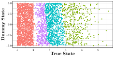
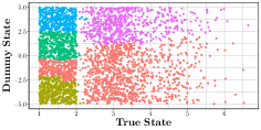
Aggregation Results To further examine the performance of state aggregation, we consider a simplified example with a two-dimensional state variable. Among the two state components, the first state is a true state and the second state is an uninformative dummy state, uniformly distributed in . The dummy state affects neither the reward nor the transition of the the first state component. We apply both ad-hoc state aggregation and SAmQ to derive state aggregation. Ideally, a good state aggregation ignores the dummy state and utilizes only the true state. The results are reported in Figure 1. We can see that SAmQ easily identifies the dummy state as the state to be discarded.
| 0.000868 | 0.000672 | 0.001242 | 0.001627 | 0.004228 | |
| 0.001674 | 0.000884 | 0.001538 | 0.002486 | 0.008288 | |
| 0.00344 | 0.011126 | 0.002502 | 0.021082 | 0.02605 |
| 0.001035 | 0.001346 | 0.000785 | 0.000744 | 0.001306 | |
| 0.002283 | 0.002542 | 0.002198 | 0.001086 | 0.003134 | |
| 0.00513 | 0.003537 | 0.013934 | 0.011486 | 0.027419 |
6.2 Airline Market Entry Analysis
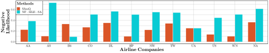
Protocol To further demonstrate the performance of SAmQ, we study airline market entry. These entry decisions are dynamic, in that entering a market generates a fixed cost. Specifically, airlines make decisions to enter markets defined as unidirectional city pairs. The state variables include origin/destination city characteristics, company characteristics, competitor information for each market and so on. We apply the considered estimation methods to the data collected and pre-processed in Berry and Jia [2010], Geng et al. [2020], Manzanares [2016]. This setting is an adaptation of the game modeled in Benkard et al. [2010]. We focus the comparison between SAmQ and NF-MLE-SA to emphasize the improvement of the proposed state aggregation scheme minimizing Q error. Since in this application, the true reward function is unknown, we compare company behaviour prediction likelihoods on hold-out test data. Figure 2 reports the results, where we see that SAmQ provides better behavioural prediction compared with the competing aggregation method for most airline companies.
6.3 Robustness to Q Estimation Error
Note that the performance of SAmQ depends on the accuracy of Q estimation. However, even when there is Q estimation error, SAmQ remains relatively robust. To demonstrate this, under the setup of Section 6.1, we added Gaussian noise with varying variances to the Q estimation in SAmQ, and report the structural parameter estimation mean squared errors (MSEs) in Table 3. As a measurement of the noise added, we use .
Importantly, our results demonstrate that SAmQ is able to provide accurate estimation even with Q function estimation errors. This is evident from the MSE values reported in Table 3, which are mostly smaller than those of the competing methods in Table 5.2. This robustness of SAmQ to Q estimation error can be attributed to the fact that SAmQ redoes DDM estimation after state aggregation, instead of purely relying on the estimated Q function. Furthermore, the robustness of SAmQ to Q estimation error explains its superior performance compared to PQR in Table 5.2. PQR relies entirely on the estimated Q function for reward estimation and is much more sensitive to Q estimation error than SAmQ.
6.4 Sample Complexity
To empirically study the sample complexity of SAmQ, we conduct additional experiments under the setting of Section 6.1, where we vary the number of data instances (as a measure of sample complexity). The results are reported in Table 4. First, given the same number of data instances , as the number of aggregated states increases, the error decreases. Second, given the same , as increases, the error does not always decrease. The reason is that when increases, the state aggregation needs to be more aggressive and aggregate more states together to achieve aggregated states. As a result, increasing without changing may hurt the estimation accuracy.
7 Conclusion and Future Work
We propose a novel DDM estimation strategy with SAmQ, state aggregation minimizing Q error. SAmQ can significantly reduce the state space, focusing only on relevant states in a data-driven way, which brings benefits in both computational and sample complexity. The proposed state aggregation method is designed by minimizing the Q error caused by aggregation, and can effectively constrain the estimation error caused by state aggregation.
One can think of a few future directions to improve the applicability and the performance of SAmQ: 1 SAmQ currently only works for exact maximum likelihood estimation. For approaches with functional approximators like many IRL techniques [Geng et al., 2020, Fu et al., 2018, Ho and Ermon, 2016], SAmQ is not guaranteed to provide performance improvements. One avenue for future work is to generalize SAmQ to such IRL methods including policy-network-based ones. 2 The current assumptions like strong concavity and full data coverage can be relaxed by further analytical techniques in offline RL [Rashidinejad et al., 2021, Lange et al., 2012, Fujimoto et al., 2019]. 3 The methodology of SAmQ can potentially be improved by aggregating states iteratively. This direction is connected to hierarchical MDP [Parr, 1998]. 4 SAmQ doesn’t rely on any prior domain knowledge. Finding ways to augment SAmQ with domain knowledge may help in specialized tasks or use-cases with little data [Nassif et al., 2009, 2012].
References
- Aguirregabiria and Mira [2002] V. Aguirregabiria and P. Mira. Swapping the nested fixed point algorithm: A class of estimators for discrete markov decision models. Econometrica, 70(4):1519–1543, 2002.
- Aguirregabiria and Mira [2007] V. Aguirregabiria and P. Mira. Sequential estimation of dynamic discrete games. Econometrica, 75(1):1–53, 2007.
- Alaluf et al. [2022] M. Alaluf, G. Crippa, S. Geng, Z. Jing, N. Krishnan, S. Kulkarni, W. Navarro, R. Sircar, and J. Tang. Reinforcement learning paycheck optimization for multivariate financial goals. Risk & Decision Analysis, 2022.
- Arcidiacono and Ellickson [2011] P. Arcidiacono and P. B. Ellickson. Practical methods for estimation of dynamic discrete choice models. Annual Review of Economics, 3(1):363–394, 2011.
- Bachem et al. [2017] O. Bachem, M. Lucic, S. H. Hassani, and A. Krause. Uniform deviation bounds for k-means clustering. In International Conference on Machine Learning, pages 283–291. PMLR, 2017.
- Bajari and Hong [2006] P. Bajari and H. Hong. Semiparametric estimation of a dynamic game of incomplete information. Technical report, National Bureau of Economic Research, 2006.
- Bajari et al. [2007] P. Bajari, C. L. Benkard, and J. Levin. Estimating dynamic models of imperfect competition. Econometrica, 75(5):1331–1370, 2007.
- Bellman [1957] R. Bellman. A markovian decision process. Journal of mathematics and mechanics, 6(5):679–684, 1957.
- Benkard et al. [2010] C. L. Benkard, A. Bodoh-Creed, and J. Lazarev. Simulating the dynamic effects of horizontal mergers: Us airlines. Manuscript, Yale University, 2010.
- Berry and Jia [2010] S. Berry and P. Jia. Tracing the woes: An empirical analysis of the airline industry. American Economic Journal: Microeconomics, 2(3):1–43, 2010.
- Bertsekas [2018] D. P. Bertsekas. Feature-based aggregation and deep reinforcement learning: A survey and some new implementations. IEEE/CAA Journal of Automatica Sinica, 6(1):1–31, 2018.
- Biswas et al. [2019] A. Biswas, T. T. Pham, M. Vogelsong, B. Snyder, and H. Nassif. Seeker: Real-time interactive search. In Proceedings of the 25th ACM SIGKDD International Conference on Knowledge Discovery and Data Mining, pages 2867–2875, 2019.
- Cirillo and Xu [2011] C. Cirillo and R. Xu. Dynamic discrete choice models for transportation. Transport Reviews, 31(4):473–494, 2011.
- Dasgupta et al. [2019] I. Dasgupta, J. Wang, S. Chiappa, J. Mitrovic, P. Ortega, D. Raposo, E. Hughes, P. Battaglia, M. Botvinick, and Z. Kurth-Nelson. Causal reasoning from meta-reinforcement learning. arXiv preprint arXiv:1901.08162, 2019.
- Dutra et al. [2011] I. Dutra, H. Nassif, D. Page, J. Shavlik, R. M. Strigel, Y. Wu, M. E. Elezaby, and E. Burnside. Integrating machine learning and physician knowledge to improve the accuracy of breast biopsy. In American Medical Informatics Association Symposium (AMIA), pages 349–355, 2011.
- Eckstein and Wolpin [1989] Z. Eckstein and K. I. Wolpin. The specification and estimation of dynamic stochastic discrete choice models: A survey. The Journal of Human Resources, 24(4):562–598, 1989.
- Ermon et al. [2015] S. Ermon, Y. Xue, R. Toth, B. Dilkina, R. Bernstein, T. Damoulas, P. Clark, S. DeGloria, A. Mude, C. Barrett, and C. P. Gomes. Learning large-scale dynamic discrete choice models of spatio-temporal preferences with application to migratory pastoralism in east africa. In AAAI Conference on Artificial Intelligence, pages 644–650, 2015.
- Feng et al. [2020] Y. Feng, E. Khmelnitskaya, and D. Nekipelov. Global concavity and optimization in a class of dynamic discrete choice models. In International Conference on Machine Learning, pages 3082–3091, 2020.
- Fiez et al. [2022] T. Fiez, S. Gamez, A. Chen, H. Nassif, and L. Jain. Adaptive experimental design and counterfactual inference. In Workshops of Conference on Recommender Systems (RecSys), 2022.
- Fu et al. [2018] J. Fu, K. Luo, and S. Levine. Learning robust rewards with adverserial inverse reinforcement learning. In International Conference on Learning Representations (ICLR), 2018.
- Fujimoto et al. [2019] S. Fujimoto, D. Meger, and D. Precup. Off-policy deep reinforcement learning without exploration. In International conference on machine learning, pages 2052–2062. PMLR, 2019.
- Geng et al. [2017] S. Geng, Z. Kuang, and D. Page. An efficient pseudo-likelihood method for sparse binary pairwise markov network estimation. arXiv preprint arXiv:1702.08320, 2017.
- Geng et al. [2018a] S. Geng, Z. Kuang, J. Liu, S. Wright, and D. Page. Stochastic learning for sparse discrete markov random fields with controlled gradient approximation error. In Uncertainty in artificial intelligence: proceedings of the… conference. Conference on Uncertainty in Artificial Intelligence, volume 2018, page 156. NIH Public Access, 2018a.
- Geng et al. [2018b] S. Geng, Z. Kuang, P. Peissig, and D. Page. Temporal poisson square root graphical models. Proceedings of machine learning research, 80:1714, 2018b.
- Geng et al. [2019a] S. Geng, Z. Kuang, P. Peissig, D. Page, L. Maursetter, and K. Hansen. Parathyroid hormone independently predicts fracture, vascular events, and death in patients with stage 3 and 4 chronic kidney disease. Osteoporosis International, 30:2019–2025, 2019a.
- Geng et al. [2019b] S. Geng, M. Yan, M. Kolar, and S. Koyejo. Partially linear additive gaussian graphical models. In International Conference on Machine Learning, pages 2180–2190. PMLR, 2019b.
- Geng et al. [2020] S. Geng, H. Nassif, C. Manzanares, M. Reppen, and R. Sircar. Deep PQR: Solving inverse reinforcement learning using anchor actions. In International Conference on Machine Learning, pages 3431–3441, 2020.
- Haarnoja et al. [2017] T. Haarnoja, H. Tang, P. Abbeel, and S. Levine. Reinforcement learning with deep energy-based policies. In International Conference on Machine Learning (ICML), pages 1352–1361, 2017.
- Hartigan and Wong [1979] J. A. Hartigan and M. A. Wong. Algorithm as 136: A k-means clustering algorithm. Journal of the royal statistical society. series c (applied statistics), 28(1):100–108, 1979.
- Hinton [2012] G. E. Hinton. A practical guide to training restricted boltzmann machines. In Neural networks: Tricks of the trade, pages 599–619. Springer, 2012.
- Ho and Ermon [2016] J. Ho and S. Ermon. Generative adversarial imitation learning. Advances in neural information processing systems, 29, 2016.
- Hotz and Miller [1993] V. J. Hotz and R. A. Miller. Conditional choice probabilities and the estimation of dynamic models. The Review of Economic Studies, 60(3):497–529, 1993.
- Hotz et al. [1994] V. J. Hotz, R. A. Miller, S. Sanders, and J. Smith. A simulation estimator for dynamic models of discrete choice. The Review of Economic Studies, 61(2):265–289, 1994.
- Huang et al. [2017] L. Huang, J. Chen, and Q. Zhu. A large-scale markov game approach to dynamic protection of interdependent infrastructure networks. In International Conference on Decision and Game Theory for Security, pages 357–376. Springer, 2017.
- Kalouptsidi et al. [2021] M. Kalouptsidi, Y. Kitamura, L. Lima, and E. Souza-Rodrigues. Counterfactual analysis for structural dynamic discrete choice models. Technical report, Working paper, Harvard University, 2021.
- Keane et al. [2011] M. P. Keane, P. E. Todd, and K. I. Wolpin. The structural estimation of behavioral models: Discrete choice dynamic programming methods and applications. In Handbook of labor economics, volume 4, pages 331–461. Elsevier, 2011.
- Kong et al. [2023] F. Kong, Y. Li, H. Nassif, T. Fiez, S. Chakrabarti, and R. Henao. Neural insights for digital marketing content design. In International Conference on Knowledge Discovery and Data Mining (KDD), 2023.
- Kuang et al. [2020] Z. Kuang, F. Sala, N. Sohoni, S. Wu, A. Córdova-Palomera, J. Dunnmon, J. Priest, and C. Ré. Ivy: Instrumental variable synthesis for causal inference. In International Conference on Artificial Intelligence and Statistics, pages 398–410. PMLR, 2020.
- Lange et al. [2012] S. Lange, T. Gabel, and M. Riedmiller. Batch reinforcement learning. In Reinforcement learning, pages 45–73. Springer, 2012.
- Li and Liu [2021] S. Li and Y. Liu. Sharper generalization bounds for clustering. In International Conference on Machine Learning, pages 6392–6402. PMLR, 2021.
- Li et al. [2022] Z. Li, L. Ratliff, H. Nassif, K. Jamieson, and L. Jain. Instance-optimal pac algorithms for contextual bandits. In Conference on Neural Information Processing Systems (NeurIPS), 2022.
- Manzanares [2016] C. A. Manzanares. Essays on the Analysis of High-Dimensional Dynamic Games and Data Combination. PhD thesis, Vanderbilt University, 2016.
- Nassif et al. [2009] H. Nassif, H. Al-Ali, S. Khuri, W. Keirouz, and D. Page. An Inductive Logic Programming approach to validate hexose biochemical knowledge. In International Conference on Inductive Logic Programming (ILP), pages 149–165, 2009.
- Nassif et al. [2012] H. Nassif, Y. Wu, D. Page, and E. S. Burnside. Logical Differential Prediction Bayes Net, improving breast cancer diagnosis for older women. In American Medical Informatics Association Symposium (AMIA), pages 1330–1339, 2012.
- Nassif et al. [2013] H. Nassif, F. Kuusisto, E. S. Burnside, D. Page, J. Shavlik, and V. Santos Costa. Score as you lift (SAYL): A statistical relational learning approach to uplift modeling. In European Conference on Machine Learning (ECML), pages 595–611, 2013.
- Parr [1998] R. E. Parr. Hierarchical control and learning for Markov decision processes. University of California, Berkeley, 1998.
- Pesaran and Smith [2016] M. H. Pesaran and R. P. Smith. Counterfactual analysis in macroeconometrics: An empirical investigation into the effects of quantitative easing. Research in Economics, 70(2):262–280, 2016.
- Rashidinejad et al. [2021] P. Rashidinejad, B. Zhu, C. Ma, J. Jiao, and S. Russell. Bridging offline reinforcement learning and imitation learning: A tale of pessimism. Advances in Neural Information Processing Systems, 34:11702–11716, 2021.
- Rust [1987] J. Rust. Optimal replacement of gmc bus engines: An empirical model of harold zurcher. Econometrica: Journal of the Econometric Society, pages 999–1033, 1987.
- Rust [1988] J. Rust. Maximum likelihood estimation of discrete control processes. SIAM journal on control and optimization, 26(5):1006–1024, 1988.
- Rust [1997] J. Rust. Using randomization to break the curse of dimensionality. Econometrica: Journal of the Econometric Society, pages 487–516, 1997.
- Singh et al. [1995] S. P. Singh, T. Jaakkola, and M. I. Jordan. Reinforcement learning with soft state aggregation. Advances in neural information processing systems, pages 361–368, 1995.
- Tsitsiklis and Van Roy [1996] J. N. Tsitsiklis and B. Van Roy. Feature-based methods for large scale dynamic programming. Machine Learning, 22(1):59–94, 1996.
- Van de Geer and van de Geer [2000] S. A. Van de Geer and S. van de Geer. Empirical Processes in M-estimation, volume 6. Cambridge university press, 2000.
- Yoganarasimhan [2018] H. Yoganarasimhan. Dynamic discrete choice models and machine learning: Methods and applications to marketing. Technical report, University of Washington, 2018.
- Zhang et al. [2020] J. Zhang, D. Kumor, and E. Bareinboim. Causal imitation learning with unobserved confounders. Advances in neural information processing systems, 33:12263–12274, 2020.
- Ziebart et al. [2008] B. D. Ziebart, A. Maas, J. A. Bagnell, and A. K. Dey. Maximum entropy inverse reinforcement learning. In Proceedings of the 23rd National Conference on Artificial Intelligence, volume 3 of AAAI’08, page 1433–1438, 2008.
Supplements
Appendix A Dynamic Discrete Choice Models in their Original Formulation
In this section, we formulate dynamic discrete choice models (DDMs) using the original formulation [Rust, 1987], and discuss its connection with the IRL formulation in Section 2.1. Note that the setup in this section is an alternative to the IRL formulation which our main results are based on and just is provided for completeness and comparison. SamQ does not require the assumptions listed in this section.
A.1 Model
Agents choose actions according to a Markov decision process described by the tuple , where
-
•
denotes the space of state variables;
-
•
represents a set of actions;
-
•
represents an agent utility function;
-
•
is a discount factor;
-
•
represents the transition distribution.
At time , agents observe state taking values in , and taking values in to make decisions. While is observable to researchers, is observable to agents but not to researchers. The action is defined as a indicator vector, , satisfying
-
•
,
-
•
takes value in .
In other words, at each time point, agents make a distinct choice over possible actions. Meanwhile, is also a representing the potential shock of taking a choice.
The agent’s control problem has the following value function:
| (10) |
where the expectation is taken over realizations of , as well as transitions of and as dictated by . The utility function can be further decomposed into
where represents the deterministic part of the utility function. Agents, but not researchers, observe before making a choice in each time period.
A.2 Assumptions and Definitions
We study DDMs under the following common assumptions.
Assumption 8.
The transition from to is independent of
Assumption 9.
The random shocks at each time point are independent and identically distributed (IID) according to a type-I extreme value distribution.
Assumption 8 ensures that unobservable state variables do not influence state transitions. This assumption is common, since it drastically simplifies the task of identifying the impact of changes in observable versus unobservable state variables. In our setting, Assumption 9 is convenient but not necessary, and could follow other parametric distributions. As pointed out by Arcidiacono and Ellickson [2011], Assumptions 8 and 9 are nearly standard for applications of dynamic discrete choice models. Such a formulation is proved to be equivalent to the IRL formulation in Section 2.1 by Geng et al. [2020], Fu et al. [2018], Ermon et al. [2015].
Appendix B Proof of Theorem 1
Proof.
By definition of and , we can derive
| (11) | ||||
where the first inequality is due to the fact that the log sum exp function is Lipschitz continuous with constant . Then, we take in Lemma 4 as , and derive
| (12) |
Proof.
By the definition of ,
| (13) |
Further, by Taylor expansion, we have
where with some . Note that the first order term is zero, since maximizes . By Assumption 1, we finish the proof.
∎
Lemma 4.
For any projection function defined in Section 3.1 and its aggregated Q function , the following inequality is true:
where is any function.
Proof.
The proof follows Theorem 3 of Tsitsiklis and Van Roy [1996]. ∎
Appendix C Proof of Theorem 2
C.1 Technical Lemmas for Theorem 2
Lemma 5.
Given , for any , we provide the following probabilistic bound for the estimated aggregated likelihood
where the expectation is over the sample .
Proof.
By inserting , we have
| (14) |
First term on the RHS of (14)
To start with, we consider . To this end, we aim to bound . We insert :
Since is a contraction with , we further derive
| (15) |
By the definition of and , it can be seen that is a sample average estimation to . Therefore, we aim to bound the difference between the two by concentration inequalities. Specifically, by assumption 6 and Hoeffding’s inequality, we have
| (16) |
Further, conditional on the event , by Hoeffding’s inequality and Assumption 7, for any
| (17) | ||||
Second term on the RHS of (14)
Now, we consider . By (11) and Assumption 7, is bounded by . Thus, by Hoeffding’s inequality, for any
Lemma 6.
Let . Then,
C.2 Proof
We first aim to bound , where the expectation is over only instead of . To this end, we insert and :
By Lemma 5 and the union bound,
Therefore,