SATR: Zero-Shot Semantic Segmentation of 3D Shapes

Abstract

We explore the task of zero-shot semantic segmentation of 3D shapes by using large-scale off-the-shelf 2D image recognition models. Surprisingly, we find that modern zero-shot 2D object detectors are better suited for this task than contemporary text/image similarity predictors or even zero-shot 2D segmentation networks. Our key finding is that it is possible to extract accurate 3D segmentation maps from multi-view bounding box predictions by using the topological properties of the underlying surface. For this, we develop the Segmentation Assignment with Topological Reweighting (SATR) algorithm and evaluate it on ShapeNetPart and our proposed FAUST benchmarks. SATR achieves state-of-the-art performance and outperforms a baseline algorithm by 1.3% and 4% average mIoU on the FAUST coarse and fine-grained benchmarks, respectively, and by 5.2% average mIoU on the ShapeNetPart benchmark. Our source code and data will be publicly released. Project webpage: https://samir55.github.io/SATR/.

1 Introduction

Recent developments in vision-language learning gave rise to many 2D image recognition models with extreme zero-shot generalization capabilities (e.g., [76, 70, 55, 54, 102]). The key driving force of their high zero-shot performance was their scale [11]: both in terms of the sheer amount of data [80, 49] and parameters [5, 97] and in terms of developing the architectures with better scalability [85, 31, 59]. However, extending this success to the 3D domain is hindered by the limited amount of available 3D data [2, 3], and also the higher computational cost of the corresponding architectural components [19]. For example, the largest openly available 2D segmentation dataset [52] contains two orders of magnitude more instance annotations than the largest 3D segmentation one [79]. This forces us to explore other ways of performing zero-shot recognition in 3D, and in our work, we explore the usage of off-the-shelf 2D models for zero-shot 3D shape segmentation.

Zero-shot 3D shape segmentation is a recently emerged research area [22] with applications in text-based editing [75, 4], stylization [65], and interactive visualization. Given a 3D mesh, the user provides one or several text descriptions of their regions of interest, and the task is to categorize each face on the mesh into one of the given descriptions (or “background” class if it does not suit any). To the best of our knowledge, the only previous work which explores this task is 3D Highlighter (3DH) [22]. The method uses an optimization-based search algorithm guided by CLIP [76] to select the necessary faces for a given text prompt. While showing strong zero-shot performance, 3DH has two drawbacks: 1) it struggles in fine-grained segmentation, and 2) it is very sensitive to initialization (see Figure 2). Moreover, due to its per-query optimization, the segmentation process is slow, taking up to ${\approx}$5-10 minutes on a recent GPU for a single semantic part.

In our work, we explore modern zero-shot 2D object detectors [55] and segmentors [54, 61] for 3D shape segmentation. Intuitively, 2D segmentation networks are a natural choice for this task: one can predict the segmentations for different views, and then directly propagate the predicted pixel classes onto the corresponding mesh faces. Moreover and surprisingly, we found that it is possible to achieve substantially higher performance using a zero-shot 2D object detector [55]. To do this, we develop Segmentation Assignment with Topological Reweighting (SATR): a method that estimates a 3D segmentation map from multi-view 2D bounding box predictions by using the topological properties of the underlying 3D surface.

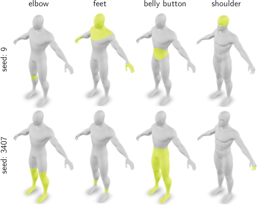
Figure 2: 3DHighlighter [23] is very sensitive to initialization. We observe that 3DHighlighter produces quite different results when using different seeds for the same prompt on different 3D shapes.

For a given mesh and a text prompt, our method first uses GLIP [55] to estimate the bounding boxes from different camera views. However, relying exclusively on the bounding boxes provides only coarse guidance for 3D segmentation and is prone to “leaking” unrelated mesh faces into the target segment. This motivates us to develop two techniques to infer and refine the proper segmentation. The first one, gaussian geodesic reweighting, performs robust reweighting of the faces based on their geodesic distances to the potential segment center. The second one, visibility smoothing, uses a graph kernel, which adjusts the inferred weights based on the visibility of its neighbors. When combined together, these techniques allow for achieving state-of-the-art results on zero-shot 3D shape segmentation, especially for fine-grained queries.

To the best of our knowledge, there are currently no quantitative benchmarks proposed for 3D mesh segmentation, and all the evaluations are only qualitative [22]. For a more robust evaluation, we propose one quantitative benchmark, which includes coarse and fine-grained mesh segmentation categories. We also evaluate our method on ShapeNetPart [95] benchmark. Our proposed benchmark is based on FAUST [9]: a human body dataset consisting of 100 real human scans. We manually segment 17 regions on one of the scans and use the shape correspondences provided by FAUST to propagate them to all the other meshes. We evaluate our approach along with existing methods on the proposed benchmarks and show the state-of-the-art performance of our developed ideas both quantitatively and qualitatively. Specifically, SATR achieves 82.46% and 46.01% average mIoU on the coarse and fine-grained FAUST benchmarks and 31.9% average mIoU scores on the ShapeNetPart benchmark, outperforming recent methods. For fine-grained categories, the advantage of our method is even higher: it surpasses a baseline method by at least 4% higher mIoU on average. We will publicly release our source code and benchmarks.

2 Related Work

Zero-shot 2D detection and segmentation. Zero-shot 2D object detection is a fairly established research area [77, 7]. Early works relied on pre-trained word embeddings [67, 74] to generalize to unseen categories (e.g., [77, 7, 25, 94]). With the development of powerful text encoders [26] and vision-language multi-modal networks [76], the focus shifted towards coupling their representation spaces with the representation spaces of object detectors (e.g.,  [38, 82]). The latest methods combine joint text, caption, and/or self-supervision to achieve extreme generalization capabilities to unseen categories (e.g,  [55, 99, 87, 102, 88, 78, 64, 35, 30]).

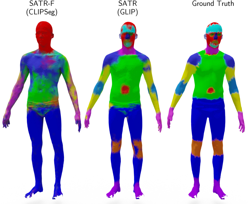
Figure 3: CLIPSeg [61] struggles to identify fine-grained parts compared to GLIP, which is a detection-based method. We show the segmented shapes using each of CLIPSeg and GLIP as a backbone for our proposed algorithm SATR. The textual prompts consist of all 17 semantic regions.

Zero-shot 2D segmentation is a more challenging problem [102] but had a similar evolutionary path to zero-shot detection. Early works (e.g., [12, 39, 6, 100, 18, 89, 71, 98]) focused on adapting open-vocabulary word embeddings to align the semantic representations with the image recognition model. Later ones (e.g., [27, 63, 54, 61, 29, 36, 62, 93, 92]) developed the mechanisms to adapt rich semantic spaces of large-scale multi-modal neural networks (e.g., [76, 70, 43]) for segmentation tasks. Some recent works show that one can achieve competitive segmentation performance using only text or self-supervision [90, 14, 13, 73, 15]. The current state-of-the-art zero-shot 2D semantic segmentation models are based on rich multi-modal supervision (e.g., [91, 99, 102]). A limiting factor of 2D segmentation is the absence of large-scale segmentation datasets due to the high annotation cost [96, 56, 51, 49], which hinders generalization. However, we observed that these models struggle to produce fine-grained segmentation even in 2D, especially for fine-grained categories (see Figure 3) and develop an algorithm that constructs accurate segmentation predictions from estimated bounding boxes.

Zero-shot 3D segmentation. Zero-shot 3D segmentation is a new research topic, and the main focus of the community was targeted towards point cloud segmentation [66, 17, 28, 57, 48]. With the rise of Neural Radiance Fields (NeRFs) [68, 60], there were several methods developed to model semantic fields(e.g., [101, 86, 32, 50, 33, 84, 83, 40, 1]) by reconstructing ground-truth or estimated semantic annotations from multi-view renderings. By distilling zero-shot 2D segmentation networks (e.g., [54, 14]) into a NeRF, these methods can perform 3D segmentation of a volumetric scene (e.g., [47, 81, 37]) and can generalize to an open-set vocabulary. By fusing representations from additional feature extractors of non-textual modalities, ConceptFusion [42] can also support zero-shot visual and audio queries. In our case, we are interested in shape segmentation and show that employing a 2D object detector yields state-of-the-art results.

PartSLIP [57] is concurrent work that performs zero/few-shot part segmentation of point clouds and, similarly to us, also relies on the GLIP [55] model. It clusters a point cloud, predicts bounding boxes via GLIP for multiple views, and assigns a score to each cluster depending on the number of its visible points inside each bounding box. Their method is designed for point clouds while ours is designed for meshes.

To the best of our knowledge, the only prior work which explores zero-shot 3D mesh segmentation is 3D Highlighter (3DH) [22]. It solves the task by optimizing a probability field of a point to match a given text prompt encoded with CLIP [76]. While showing strong generalization capabilities, their approach struggles to provide fine-grained predictions and is very sensitive to initialization (see Figure 2).

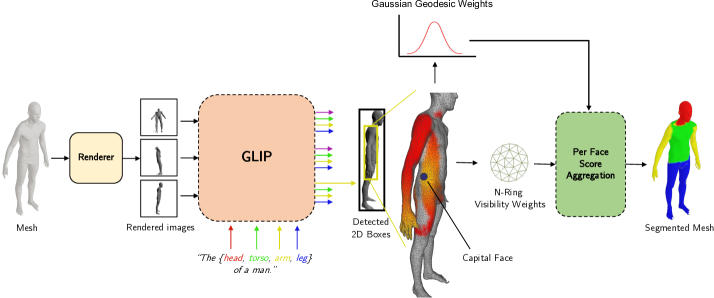
Figure 4: An overview of our method. Meshes are rendered from random viewpoints. The resulting images are processed by GLIP, which detects bounding boxes in the images. Each bounding box corresponds to a prompt (segment). For each bounding box, we compute scores for triangles inside the bounding box using Gaussian Geodesic Reweighting and Visibility Smoothing. Aggregating the scores yields a segmented mesh.

3 Method

As input, we assume a 3D shape, represented as a polygon mesh $\mathcal{F}=\{\bm{f}_{n}\}_{i=n}^{N}$ of $d$-sided polygon faces $\bm{f}_{n}\in\mathbb{R}^{d\times 3}$, and $K$ semantic text descriptions $\{\bm{t}_{k}\}_{k=1}^{K}$, provided by the user. The prompts $\bm{t}_{k}$ are single nouns or compound noun phrases consisting of multiple words. Then, the task of 3D shape segmentation is to extract $K$ non-intersecting subsets $\{\mathcal{F}_{k}\ |\ \mathcal{F}_{k}\subseteq\mathcal{F}\}_{k=1}^{K}$ in such a way that the $k$-th subset $\mathcal{F}_{k}$ is a part of the mesh surface which semantically corresponds to the $k$-th text prompt $\bm{t}_{k}$.

In our work, we explore modern powerful 2D vision-language models to solve this task. The simplest way to incorporate them would be employing a zero-shot 2D segmentation network, like CLIPSeg [61] or LSeg [54], which can directly color the mesh given its rendered views. But as we show in experiments, this leads to suboptimal results since modern zero-shot 2D segmentors struggle to produce fine-grained annotations and high-quality segments, while 2D detectors could be adapted for shape segmentation with surprisingly high precision.

In our work, we consider untextured meshes, but it is straightforward to apply the method to textured ones.

In this way, our method relies on a zero-shot 2D object detector $\mathsf{D}(\bm{x},\bm{t})=\{(\bm{b}_{\ell},p_{\ell})\}_{\ell=1}^{L}$, which takes as input an RGB image $\bm{x}\in\mathbb{R}^{H\times W\times 3}$ of size $H\times W$ and a text prompt $\bm{t}$, and outputs $L\geq 0$ bounding boxes $\bm{b}_{\ell}=(x_{\ell},y_{\ell},h_{\ell},w_{\ell})\in\mathbb{R}^{4}$ with their respective probability scores $p_{\ell}\in[0,1]$. In our notation, each bounding box $\bm{b}_{\ell}$ is defined by its left lower corner coordinate $(x_{\ell},y_{\ell})$, width $w_{\ell}$, and height $h_{\ell}$. We choose GLIP [55] as the detector model due to its state-of-the-art generalization capabilities.

In this section, we first describe a topology-agnostic baseline framework (denoted as SATR-F) that can leverage a 2D object detector to segment a meshed 3D surface. Then, we explain why it is insufficient to infer accurate segmentation predictions (which is also confirmed by the experiments in Tables 1, 2 and 3) due to the coarse selection nature of the bounding boxes. After that, we develop our Segmentation Assignment with Topological Reweighting (denoted as SATR (F+R) or SATR in short) algorithm, which alleviates this shortcoming by using the topological properties of the underlying surface.

3.1 Topology-Agnostic Mesh Segmentation

Our topology-agnostic baseline method works the following way. We render the mesh $\mathcal{F}$ from $M$ random views (we use $M=10$ in all the experiments, if not stated otherwise) to obtain RGB images $\bm{x}_{m}$. To create the $M$ views, we generate random camera positions where the elevation and azimuth angles are sampled using the normal distribution ($\mu=0.7$,$\sigma=4$). We use this view generation to be directly comparable to 3DHighlighter [22]. After that, for each view $\bm{x}_{m}$ and for each text prompt $\bm{t}_{k}$, we use the detector model to predict the bounding boxes with their respective confidence scores:

$$\{(\bm{b}_{\ell}^{m,k},p_{\ell}^{m,k})\}_{\ell=1}^{L_{m,k}}=\mathsf{D}(\bm{b}_{m},\bm{t}_{k}).$$ (1)

Then, we use them to construct the initial face weights matrix $\mathcal{W}^{\prime}_{m}\in[0,1]^{N\times K}$ for the $m$-th view. Let $\mathcal{F}_{\ell}^{m,k}\subseteq\mathcal{F}$ denote a subset of visible (in the $m$-th view) faces with at least one vertex inside bounding box $\ell^{m,k}$, whose projection falls inside $\bm{b}_{\ell}^{m,k}$. Then

$$\mathcal{W}_{m}[n,k]=\sum_{\ell=1}^{L_{m,k}}{\mathcal{W}^{\ell}_{m}[n,k,\ell]}$$ (2)

$$\mathcal{W}^{\ell}_{m}[n,k,l]=\begin{cases}p_{\ell}^{m,k}&~{}\text{if $\bm{f}_{n}\in\mathcal{F}_{\ell}^{m,k}$}\\ 0&~{}\text{otherwise.}\end{cases}$$ (3)

In this way, the score of each face $\bm{f}_{n}$ for the $m$-th view is simply set to the confidence $p_{\ell}^{m,k}$ of the corresponding bounding box(es) it fell into.

The face visibility is determined via the classical $Z$-culling algorithm [34]. In this way, if there are no bounding boxes predicted for $\bm{x}_{m}$ for prompt $\bm{t}_{k}$, then $\mathcal{W}_{m}[n,k]$ equals the zero matrix. The latter happens when the region of interest is not visible from a given view or when the detector $\mathsf{D}$ makes a prediction error.

Next, we take into account the area sizes of each face projection. If a face occupies a small area inside the bounding box, then it contributed little to the bounding box prediction. The area $s_{m,\ell}^{n}$ of the face $\bm{f}_{n}$ in the view $\bm{x}_{m}$ and bounding box $\ell$ is computed as the number of pixels which it occupies. We use the computed areas to re-weight the initial weights matrix $\mathcal{W}^{\prime}_{m}$ and obtain the area-adjusted weights matrix $\mathcal{W}_{m}\in\mathbb{R}^{N\times K}$ for the $m$-th view:

$$\mathcal{W}_{m}[n,k]=\sum_{\ell=1}^{L_{m,k}}{\mathcal{W}^{\ell}_{m}[n,k,\ell]\times s_{m,\ell}^{n}}$$ (4)

To compute the final weights matrix, we first aggregate the predictions from each view $\bm{x}_{m}$ by summing the scores of the un-normalized matrix $\tilde{\mathcal{W}}\in\mathbb{R}^{N\times K}$:

$$\tilde{\mathcal{W}}[n,k]=\sum_{m}{\mathcal{W}_{m}[n,k]},$$ (5)

and then normalize it by dividing each column by its maximum value to obtain our final weights matrix $\mathcal{W}\in\mathbb{R}^{N\times K}$:

$$\mathcal{W}[n,k]=\tilde{\mathcal{W}}[n,k]/\max_{k}\tilde{\mathcal{W}}[n,k].$$ (6)

The above procedure constitutes our baseline method of adapting bounding box predictions for 3D shape segmentation. As illustrated in Figure 8, its disadvantage is “segmentation leaking”: some semantically unrelated parts of the surface get incorrectly attributed to a given text prompt $\bm{t}$, because they often fall into predicted bounding boxes from multiple views. To alleviate this issue, we develop a more careful score assignment algorithm that uses the topological properties of the surface, thus allowing us to obtain accurate 3D shape segmentation predictions from a 2D detector.

3.2 Gaussian Geodesic Reweighting

Bounding box estimates give only coarse estimates about the semantic region being queried, and we found that using the surface topology allows localizing it with substantially better precision. For this, we construct a method that utilizes geodesic distances between mesh faces, i.e., path lengths from one face to another along the surface, instead of their direct distances in Euclidian space.

Consider the following example of segmenting a human palm. When the hand is in a resting state, the palm lies close to the waistline in Euclidean space (as illustrated in Figure 5). Then, a simple topology-agnostic method would lead to the waistline leaking into the segmentation prediction. At the same time, one can observe that the predicted bounding boxes are always centered around the palm, and the waistline is far away from it in terms of the geodesic distance. In this way, discarding such outlying polygons yields a precise segmentation of the required region. And this is the main intuition of our developed algorithm.

As a first step, for each predicted bounding box $\bm{b}_{\ell}^{m,k}$, we estimate its central face, which we call the capital face $g^{m,k}_{\ell}\in\mathcal{F}$. It is computed by taking the (area-weighted) average of all the vertices from all the faces inside $\mathcal{F}_{\ell}^{m,k}$, projecting this average point onto $\mathcal{F}$ and taking the face on which the projection lies. After that, we compute a vector of geodesic distances $\bm{d}_{\ell}^{m,k}\in\mathbb{R}_{+}^{N}$ from the capital face $g^{m,k}_{\ell}$ to every other face $f\in\mathcal{F}_{\ell}^{m,k}$:

$$\bm{d}_{\ell}^{m,k}[n]=\begin{cases}\text{gdist}(g_{\ell}^{m,k},\bm{f}_{n})&\text{if~{}}\bm{f}_{n}\in\mathcal{F}_{\ell}^{m,k}\\ 0&\text{otherwise}\end{cases}$$ (7)

where $\text{gdist}(\cdot,\cdot)$ denotes the geodesic length between two faces computed on the mesh $\mathcal{F}$ using the Heat method [21].

It feels natural to use those geodesic distances directly to reweight the original weight matrix $\mathcal{W}$. However, this leads to sub-optimal results for two reasons: 1) there are natural errors in selecting the capital face, which would bias reweighting towards incorrect regions; and 2) as we show in Figure 5, it is difficult to tune the decay rate for such reweighting. Instead, we propose Gaussian reweighting and demonstrate that it is more robust and accurate in practice. It works the following way.

First, we fit a Gaussian distribution over the distances and compute the corresponding probability density values for each face given its geodesic distance from the capital face:

$$\bm{r}_{\ell}^{m,k}\triangleq\{\mathcal{N}(d;\mu_{\ell}^{m,k},(\sigma_{\ell}^{m,k})^{2})\ |\ d\in\bm{d}_{\ell}^{m,k}\},$$ (8)

where $\mu_{\ell}^{m,k},\sigma_{\ell}^{m,k}$ denote the mean and standard deviation of the distances $\bm{d}_{\ell}^{m,k}$. This formulation nudges the weights away from the capital and works like adaptive regularization. If there are inaccuracies in the capital face selection, then it will have less influence on the segmentation quality. We aggregate the weights from multiple views into a single vector of scores $\bm{r}^{m,k}\in\mathbb{R}_{+}^{N}$ and reweigh the original weight matrix $\mathcal{W}_{m}$ for the $m$-th view to obtain the weight matrix $\mathcal{W}_{m}^{g}$ with Gaussian geodesic reweighting:

$$\mathcal{W}_{m}^{g}[n,k]=\sum_{\ell=1}^{L_{m,k}}{\mathcal{W}^{\ell}_{m}[n,k,\ell]\times s_{m,\ell}^{n}\times\bm{r}_{\ell}^{m,k}}.$$ (9)

After that, we compute the final weight matrix $\mathcal{W}^{g}\in\mathbb{R}^{N\times K}$ for each face $\bm{f}_{n}\in\mathcal{F}$ in a similar manner to $\mathcal{W}$ by taking the summing over $\mathcal{W}_{m}^{g}$ from different views. We find that not normalizing the weight matrix whenever the Gaussian Geodesic Reweighting is used yields better performance than applying normalization.

This procedure takes into account the topological structure of the mesh surface, which allows for obtaining more accurate segmentation performance, as can be seen from Tables 2 and 1 and Figure 7. However, it has one drawback: it pushes the weights away from the capital face, which might decrease the performance. To compensate for this, we develop the technique of visibility smoothing, which we describe next.

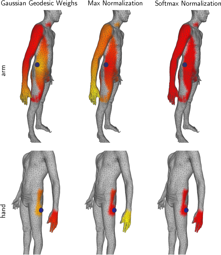
Figure 5: Gaussian Geodesic Weights can help reduce the scores for triangles inside a detected bounding box that do not belong to the segment of the corresponding text prompt.

3.3 Visibility Smoothing

The score matrix $\mathcal{W}^{g}$ with Gaussian geodesic reweighting might allocate too little weight on the central faces around the capital face $g_{\ell}^{m,k}$, which happens for regions with a large average distance between the faces. To compensate for this, we propose visibility smoothing. It works independently in the following way.

For each visible face $\bm{f}\in\mathcal{F}_{\ell}^{m,k}$, we compute its local neighborhood, where the neighbors are determined via mesh connectivity: a face $\bm{g}$ is a neighbor of face $\bm{f}$ if they share at least one vertex. For this, we use a $q$-rank neighborhood $\mathcal{N}_{q}(\bm{f})$ (we use $q=5$ in all the experiments unless stated otherwise), which is constructed the following way. For face $\bm{f}_{n}\in\mathcal{F}$, we take the face $\bm{g}\in\mathcal{F}$ if there exists a path on a graph between $\bm{f}$ and $\bm{g}$ of at most $q$ other vertices.

After that, we compute the neighborhood visibility scores vector $\bm{v}_{\ell}^{m,k}\in[0,1]^{N}$ for each face $\bm{f}_{n}\in\mathcal{F}$ by computing the ratio between visible faces in its neighborhood and the overall neighborhood size:

$$\bm{v}_{\ell}^{m,k}[n]=\frac{|\mathcal{N}_{q}(\bm{f}_{n})\cap\mathcal{F}_{\ell}^{m,k}|}{|\mathcal{N}_{q}(\bm{f}_{n})|}.$$ (10)

Similarly to geodesic weighting, we aggregate the neighborhood visibility scores $\bm{v}_{\ell}^{m,k}[n]$ across the bounding boxes into $\bm{v}^{m,k}[n]\in[0,1]^{N}$ via element-wise vector summation:

$$\bm{v}^{m,k}[n]=\sum_{\ell=1}^{L}\bm{v}^{m,k}_{\ell}[n]$$ (11)

This gives us our final per-view score matrix $\mathcal{W}_{m}^{*}\in\mathbb{R}_{+}^{N\times K}$:

$$\mathcal{W}_{m}^{*}[n,k]=\sum_{\ell=1}^{L_{m,k}}{\mathcal{W}^{\ell}_{m}[n,k,\ell]\times s_{m,\ell}^{n}\times\bm{r}_{\ell}^{m,k}\times\bm{\bm{v}}^{m,k}[n]}.$$ (12)

Again, we aggregate our multi-view scores $\mathcal{W}_{m}^{*}[n]$ into the final weights matrix $\mathcal{W}^{*}[n]$ by taking the maximum across the views.

We call the above technique visibility smoothing since it smoothes face weights according to their neighborhood visibility and can be seen as a simple convolutional kernel over the graph. It allows for repairing the weights in the central part of the visible surface region without damaging the rest of the faces. This consequently leads to a noticeable improvement in the scores, as we report in Tables 5 and 1.

The pseudo-code of our algorithm is provided in Algorithm 1 in Appx B, together with additional implementation details. Also, note that the source code of our method will be publicly released.

4 Experiments

Figure 6: Proposed FAUST Benchmark. It contains 100 human shapes with both coarse and fine-grained annotations.

4.1 Experimental Setup

Method	Backbone	mIoU	arm	belly button	chin	ear	elbow	eye	foot	fore- head	hand	head	knee	leg	mouth	neck	nose	shou- lder	torso
3DH [23]	CLIP [76]	3.89	18.39	1.99	0.46	0.72	0.08	0.0	20.81	0.70	0.02	3.49	6.17	3.91	0.05	1.94	0.07	0.04	7.28
SATR-F	CLIPSeg	10.88	11.51	0.10	0.30	0.0	0.03	0.0	03.28	0.0	25.80	39.99	0.07	50.52	0.0	0.05	0.0	5.11	48.24
	GLIP	41.96	45.22	26.30	37.68	41.67	24.93	25.95	53.94	41.63	68.22	42.56	32.69	59.73	27.59	41.78	50.57	33.00	59.83
SATR	GLIP	46.01	50.51	29.41	27.74	47.45	26.80	18.90	81.99	38.11	81.45	51.11	33.34	65.22	27.29	41.95	57.60	38.94	64.35

Table 1: Performance of SATR on the fine-grained semantic segmentation on FAUST dataset.

	Backbone	mIoU	arm	head	leg	torso
3DH [23]	CLIP [76]	16.50	28.60	14.20	14.90	8.20
SATR-F	LSeg [54]	6.50	26.00	0.0	0.0	0.0
	CLIPSeg [61]	60.34	46.55	58.01	76.22	59.80
	GLIP [55]	81.16	82.01	88.17	86.54	67.92
SATR	GLIP [55]	82.46	85.92	90.56	85.75	67.60

Table 2: Performance of SATR on the coarse-grained semantic segmentation on FAUST dataset.

Datasets and splits. We evaluate the zero-shot performance on our proposed FAUST [9] benchmark and on the ShapeNetPart  [95] dataset. For the FAUST dataset, we use all of the 100 scans available. We manually collected the coarse and fine-grained annotations in the following way. First, we manually annotate the registered mesh of one human scan as shown in Figure 6 using vertex paint in Blender [8]. Since we have access to the FAUST mesh correspondences, we are able to transfer our annotations to all other scans. We then re-mesh each human scan independently to contain around 20K triangular faces. To generate annotations for these re-meshed scans, we assign the label of each vertex to the label of the nearest vertex before remeshing. For the ShapeNetPart dataset [95], it contains 16 object categories and 50 annotated parts for shapes from the ShapeNet [16] dataset. We use all of the 2460 labeled shapes of the ShapeNetPart dataset provided by [44], where the point labels are transferred to mesh polygon labels via a nearest neighbors approach combined with graph cuts. The meshes in ShapeNetPart have triangular faces that are very large, covering a large portion of the mesh surface. For this reason, during model inference, we provide re-meshed ShapeNetPart shapes as input, where each mesh contains at most 30K triangular faces. We use the Isotropic Explicit Remeshing algorithm [41] provided by MeshLab [20] to do the re-meshing. During the evaluation, we transferred the predicted face labels back to the original ShapeNetPart shapes. Figure 1 includes examples from the TextANIMAR [53], Objaverse [24], and TOSCA [10] datasets.

Metrics. We use the semantic segmentation mIoU as described in [69]. We first calculate the mIoU for each part category across all the test shapes and then compute for each object category the average of the part mIoU.

4.2 Implementation Details

We use a single Nvidia V100 GPU for each experiment. We use the Nvidia Kaolin library [34] written in PyTorch [72] for rendering in all of our experiments. To ensure fairness, we use the same views in all of our GLIP-based model experiments. As a pre-processing step, we center the input mesh around the origin and normalize it inside a unit sphere. For rendering, we use a resolution of $1024\times 1024$ and a black background color.

4.3 Zero-Shot Semantic Segmentation

4.3.1 FAUST Benchmark

We compare our method with 3DHighlighter [22] and CLIPSeg [61]. To obtain semantic segmentation results from 3DHighlighter, we run the optimization separately to get a highlighted mesh for each of the input semantic regions. If a face were highlighted for different semantic regions, its predicted label would be the semantic class with the highest CLIP similarity score. To obtain semantic segmentation results from CLIPSeg, we generate a segmentation mask for each rendered view for each semantic label, and we aggregate the segmentation scores for each face and assign the most predicted label for each face.

In Table 2, we report the overall average mIoU and the mIoU for each semantic part on our proposed FAUST benchmark. SATR significantly outperforms 3DHighlighter on the coarse-grained parts. As shown in Figure 7, our method SATR outperforms 3DHighlighter and CLIPSeg on all of the four semantic parts (leg, arm, head, and torso) by an overall average mIoU of 82.46%. In addition, we show that our proposed components(SATR) help improve the results upon our GLIP-based baseline (SATR-Baseline). In Figure 7, we show the qualitative results of our method, and we compare it to 3DHighlighter. In addition, in Table 1, our method SATR overall outperforms 3DHighlighter with a margin of 42.12% in the fine-grained semantic segmentation. In Figure 7, we show the results of SATR on fine-grained segmentation compared to the ground truth.

Figure 7: Qualitative results and comparison between 3DHighlighter, SATR-F, and SATR

Method	Backbone	mIoU	air- plane	bag	cap	car	chair	ear- phone	guitar	knife	lamp	laptop	motor- bike	mug	pistol	rocket	skate- board	table
3DH [23]	CLIP [76]	5.70	5.81	2.05	2.85	2.88	15.53	9.55	0.86	1.58	13.21	1.78	5.57	0.65	1.36	10.36	6.44	10.77
SATR-F	GLIP [55]	26.67	41.73	26.60	22.96	22.01	26.61	14.95	43.55	30.79	31.16	30.05	12.40	31.55	19.63	15.55	34.49	22.70
SATR	GLIP [55]	31.90	38.46	44.56	24.01	19.62	33.16	16.90	40.22	45.92	30.22	37.79	15.70	52.31	20.87	28.41	30.77	31.41

Table 3: Performance of SATR on the ShapeNetPart dataset.

4.3.2 ShapeNetPart Dataset

In Table 3, SATR consistently outperforms 3DHighlighter in every shape category by a large margin. The results suggest that our proposed method SATR is applicable not only to human shapes but can also perform well in a wide range of categories. In Figure 7, we compare SATR and 3DHighlighter. The main challenge is that 3DHighlighter only works with the right random initialization, which doesn’t happen too often.

4.4 Ablation Studies

Effectiveness of the proposed components. We ablate the effectiveness of our proposed components for FAUST coarse and fine-grained benchmarks in Tables 7 and 5. Using both Gaussian geodesic re-weighting and visibility smoothing gave the best performance in both the coarse and fine-grained FAUST benchmarks. In addition, each component is effective on its own and performs better than SATR-Baseline. The results suggest that both components work in a complementary fashion.

Method	Backbone(s)	Coarse-Grained mIoU	Fine-Grained mIoU
SATR-F	GLIP [55]	81.16	41.96
	GLIP-SAM [45]	78.59	27.52
	DINO-SAM [14]	80.42	21.90
SATR	GLIP [55]	82.46	46.01

Table 4: mIoU comparison between SATR and SATR-F with recent SAM-based [46] backbones.

Gaussian Geod- esic Reweighting	Visibility Smoothing	mIoU	arm	head	leg	torso
		81.16	82.01	88.17	86.54	67.92
	✓	81.69	82.68	88.61	86.85	68.61
✓		82.39	85.73	90.61	85.81	67.41
✓	✓	82.46	85.92	90.56	85.75	67.60

Table 5: Ablation to show the effectiveness of our proposed components for the coarse-grained FAUST benchmark.

Re-weighting Method	Coarse-Grained mIoU	Fine-Grained mIoU
Max Geodesic	82.41	44.57
Softmax Geodesic	81.69	43.34
Gaussian Geodesic (ours)	82.46	46.01

Table 6: Ablation on using different re-weighting methods. Our proposed Gaussian Geodesic Re-weighting method outperforms other normalization methods. This shows its effectiveness in the fine-grained and more difficult semantic segmentation task.

Different reweighting methods. We compare using different re-weighting methods as shown in Table 6. As discussed earlier in Section 3.2, we compute the geodesic distances between every visible face in a predicted bounding box and the capital face. To compute the weights for every visible face, we try re-weighting by doing the following $w_{i}=(1-dist_{i}/(max_{dist}+\epsilon))$. We also try computing the weights by normalizing the distance with a softmax function. Our proposed Gaussian geodesic re-weighting method outperforms other methods, especially in the fine-grained benchmark with a very large margin, showing that it is robust when the capital face is miscalculated.

Figure 8: Segmentation leaking problem. Some semantically unrelated parts of the surface get incorrectly attributed to a given textual prompt because they often fall into predicted bounding boxes from multiple views.

Comparison using recent 2D segmentation models. Recent foundation models for 2D semantic segmentation show promising results for zero-shot 2D semantic segmentation. For instance, SAM [46] can be combined with powerful 2D object detectors (like GLIP [55] and Grounding-DINO[58]) for text-based semantic segmentation. In Table 4, we compare our proposed method with DINO-SAM and GLIP-SAM based segmentation methods. Our proposed object detector-based method still exhibits strong performance among recent works, especially in the FAUST fine-grained benchmark.

Gaussian Geodesic Reweighting	Visibility Smoothing	mIoU
		41.96
	✓	43.35
✓		45.56
✓	✓	46.01

Table 7: Ablation on trying all the possible combinations of our proposed components for the fine-grained FAUST benchmark.

5 Conclusion

In our work, we explored the application of modern zero-shot 2D vision-language models for zero-shot semantic segmentation of 3D shapes. We showed that modern 2D object detectors are better suited for this task than text-image similarity or segmentation models, and developed a topology-aware algorithm to extract 3D segmentation mapping from 2D multi-view bounding box predictions. We proposed the first benchmarks for this area. We compared to previous and selected concurrent work qualitatively and quantitatively and observed a large improvement when using our method. In future work, we would like to combine different types of language models and investigate in what way the names of the segments themselves can be proposed by a language model. We discuss the limitations of our approach in Appx A.

Appendix A Limitations

In this section, we discuss the limitations of our approach. First, there is no formal guarantee that the random view sampling algorithm covers each triangle. We mainly used this choice to be compatible with previous work. Alternatively, one could devise a greedy view selection algorithm that ensures each triangle is selected once. Another approach would be to use a set of uniformly distributed viewpoints that are fixed for the complete dataset. Second, we are not able to test other types of large language models because the latest versions are not publicly available [99]. Third, GLIP prediction is not perfect. For example, it can incorrectly detect parts that are semantically different but still look similar (for instance, the front and the backpack of an astronaut, see Figure 1).

Appendix B SATR Pseudocode

In Algorithm 1, we show the pseudocode of our proposed method (SATR).

Input : Zero-shot 2D object detector $D(\bm{x},\bm{t})$, where $x$ is an image and $t$ is a text prompt.

Input : Shape surface as a mesh of faces $\mathcal{F}$.

Input : Set of textual prompts $\mathcal{T}$ representing semantic regions/classes.

Input : Number of views $N_{views}$

Input : The q-ring neighborhood $q$.

Output : The predicted semantic label of each face of the input mesh $\mathcal{F}$.

# Initialize face scores

$S$ = zeros($\mathcal{F}$.faces.length, $\mathcal{T}$.length),

# Compute the pair-wise geodesic distance between every pair of faces

$G$ = computeFacePairwiseDistance($\mathcal{F}$)

# Find the $q$-ring neighborhood for all the faces of the mesh

$Q$ = getFaceQNeighbors($\mathcal{F}$, q)

# Render the mesh

$V$, Pixel2Face = renderMesh($\mathcal{F}$, $N_{views}$)

for $v$ in $V$ do

       for $t$ in $\mathcal{T}$ do

             # Detect 2D Bounding Boxes for the given $t$ prompt

             $B_{v,t}$ = predictBoxes($v$, $t$)

             for $b_{t,v}$ in $B_{v,t}$ do

                   # Get the visible faces inside $b_{t,v}$

                   $f_{t,v}$ = getVisibleFaces($b_{t,v}$, $\mathcal{F}$, Pixel2Face)

                  

                  # Compute capital face

                   $c$ = computeCapitalFace($f_{t,v}$, $\mathcal{F}$)

                  # Compute frequency of the visible faces

                   $w_{freq}$ = faceFreq($f_{t,v}$, Pixel2Face)

                  # Compute Gaussian Geodesic weights

                   $w_{geo}$ = faceGeodesicWeights($c$, $f_{t,v}$)

                  # Compute visibility smoothing weights

                   $w_{vis}$ = faceVisibilityWeights($f_{t,v}$, $Q$)

                  # Update face scores

                   $S_{f_{t,v},i_{t}}$ += $w_{geo}$ * $w_{vis}$ * $w_{freq}$

                  

             end for

            

       end for

      

end for

face_label = argMax($S$, axis=1)

Return face_label;

Algorithm 1 Segmentation Assignment with Topological Reweighting (SATR) in highlevel pseudocode.

	Coarse-Grained mIoU	Fine-Grained mIoU
Uniform Sampling	81.58	43.76
Sampling using Normal Distribution [23]	82.46	46.01

Table 1: Ablation on using different view-port sampling methods in our proposed method SATR on FAUST coarse and fine-grained benchmarks. (with ten rendered views as input).

Appendix C Additional Ablation Studies

C.1 Changing the Number of Views

We investigate the effect of changing the number of input rendered views on our proposed method SATR. In Table 3, we report the mIoU performance on both the coarse and the fine-grained FAUST benchmarks. Generally, increasing the number of views results in better segmentation performance in both benchmarks. However, the computation time increases, and there are diminishing returns for adding a large number of views.

C.2 Camera View-port Sampling Approach

We ablate using different sampling approaches for choosing the camera view-ports. In Table 1, we compare between sampling camera view-ports using the approach described in [22] and doing uniform viewpoint sampling using a range of equidistant elevation and azimuth angles. We report the mIoU performance on both the coarse and the fine-grained FAUST benchmarks. We observe that sampling from a normal distribution ($\mu=3.14$, $\sigma=4$) results in better performance in both benchmarks. The reason behind this is having more control over the range of the elevation and azimuth angles can produce better views that cover most of the input mesh and avoid sampling views where a lot of occlusions may happen. More complex view selection could be future work.

Figure 1: GLIP model can incorrectly detect semantically different parts that look similar. Since the parts of the astronaut suit look similar, GLIP mistakenly predicts the astronaut’s chest as a part of the backpack and doesn’t predict a tighter bounding box around the backpack.

	Coarse-Grained mIoU	Fine-Grained mIoU
Red	80.62	40.67
Blue	81.35	42.58
Skin color	82.22	44.58
Gray	82.46	46.01

Table 2: Ablation on changing the vertex colors of the input 3D models to our proposed method SATR on FAUST coarse and fine-grained benchmarks. (with ten rendered views as input).

# Views	Coarse-Grained mIoU	Fine-Grained mIoU
5	53.99	25.96
10	82.46	24.3
15	80.48	43.40
20	82.41	45.20
30	84.06	47.87
40	84.26	47.67

Table 3: Ablation on using a different number of rendered views as input to our proposed method SATR on FAUST coarse and fine-grained benchmarks.

C.3 Coloring The Input Mesh

We ablate the effect of changing the color of the input mesh on the performance of SATR. We run three experiments by using four different colors for the input meshes; grey, red, blue, and natural skin color. As shown in Table 2, we find that using the gray color results in the best performance compared to other colors.

	Backbone	Coarse-mIoU	Fine-mIoU
SATR-F	GLIP [55]	81.16	41.96
SATR (add)	GLIP [55]	82.75	44.90
SATR (mul)	GLIP [55]	82.46	46.01

Table 4: Ablation on different ways of combining the reweighting factors.

C.4 Summation of Reweighting Factors

We replace the multiplication of both of the Gaussian Geodesic and Visiblity Smoothing reweighting factors as shown in Equation 12 with addition:

$$\mathcal{W}_{m}^{*}[n,k]=\sum_{\ell=1}^{L_{m,k}}{\mathcal{W}^{\ell}_{m}[n,k,\ell]\times s_{m,\ell}^{n}\times\bm{(}r_{\ell}^{m,k}+\bm{\bm{v}}^{m,k}[n]}).$$ (13)

We show the mIoU performance on both FAUST coarse and fine-grained benchmarks in Table 4. The addition of the reweighting factors gave slight increase in performance for the coarse benchmark while perform significantly worse than multiplying the reweighting factors.

References

- [1] Ahmed Abdelreheem, Abdelrahman Eldesokey, Maks Ovsjanikov, and Peter Wonka. Zero-shot 3d shape correspondence, 2023.
- [2] Ahmed Abdelreheem, Kyle Olszewski, Hsin-Ying Lee, Peter Wonka, and Panos Achlioptas. ScanEnts3D: Exploiting phrase-to-3d-object correspondences for improved visio-linguistic models in 3d scenes. arXiv, abs/2212.06250, 2022.
- [3] Panos Achlioptas, Ahmed Abdelreheem, Fei Xia, Mohamed Elhoseiny, and Leonidas J. Guibas. ReferIt3D: Neural listeners for fine-grained 3d object identification in real-world scenes. In ECCV, 2020.
- [4] Panos Achlioptas, Ian Huang, Minhyuk Sung, Sergey Tulyakov, and Leonidas Guibas. ShapeTalk: A language dataset and framework for 3d shape edits and deformations. Proceedings of the IEEE Conference on Computer Vision and Pattern Recognition, 2023.
- [5] Jean-Baptiste Alayrac, Jeff Donahue, Pauline Luc, Antoine Miech, Iain Barr, Yana Hasson, Karel Lenc, Arthur Mensch, Katie Millican, Malcolm Reynolds, et al. Flamingo: a visual language model for few-shot learning. arXiv preprint arXiv:2204.14198, 2022.
- [6] Donghyeon Baek, Youngmin Oh, and Bumsub Ham. Exploiting a joint embedding space for generalized zero-shot semantic segmentation. In ICCV, 2021.
- [7] Ankan Bansal, Karan Sikka, Gaurav Sharma, Rama Chellappa, and Ajay Divakaran. Zero-shot object detection. In Proceedings of the European Conference on Computer Vision (ECCV), pages 384–400, 2018.
- [8] Blender Online Community. Blender - a 3D modelling and rendering package. Blender Foundation, Blender Institute, Amsterdam, 2022.
- [9] Federica Bogo, Javier Romero, Matthew Loper, and Michael J Black. Faust: Dataset and evaluation for 3d mesh registration. In Proceedings of the IEEE conference on computer vision and pattern recognition, pages 3794–3801, 2014.
- [10] Alexander M. Bronstein, Michael M. Bronstein, and Ron Kimmel. Numerical geometry of non-rigid shapes. In Monographs in Computer Science, 2009.
- [11] Tom Brown, Benjamin Mann, Nick Ryder, Melanie Subbiah, Jared D Kaplan, Prafulla Dhariwal, Arvind Neelakantan, Pranav Shyam, Girish Sastry, Amanda Askell, et al. Language models are few-shot learners. Advances in neural information processing systems, 33:1877–1901, 2020.
- [12] Maxime Bucher, Tuan-Hung Vu, Matthieu Cord, and Patrick Pérez. Zero-shot semantic segmentation. Advances in Neural Information Processing Systems, 32, 2019.
- [13] Ryan Burgert, Kanchana Ranasinghe, Xiang Li, and Michael S Ryoo. Peekaboo: Text to image diffusion models are zero-shot segmentors. arXiv preprint arXiv:2211.13224, 2022.
- [14] Mathilde Caron, Hugo Touvron, Ishan Misra, Hervé Jégou, Julien Mairal, Piotr Bojanowski, and Armand Joulin. Emerging properties in self-supervised vision transformers. In Proceedings of the IEEE/CVF international conference on computer vision, pages 9650–9660, 2021.
- [15] Junbum Cha, Jonghwan Mun, and Byungseok Roh. Learning to generate text-grounded mask for open-world semantic segmentation from only image-text pairs. arXiv preprint arXiv:2212.00785, 2022.
- [16] Angel X Chang, Thomas Funkhouser, Leonidas Guibas, Pat Hanrahan, Qixing Huang, Zimo Li, Silvio Savarese, Manolis Savva, Shuran Song, Hao Su, et al. Shapenet: An information-rich 3d model repository. arXiv preprint arXiv:1512.03012, 2015.
- [17] Runnan Chen, Xinge Zhu, Nenglun Chen, Wei Li, Yuexin Ma, Ruigang Yang, and Wenping Wang. Zero-shot point cloud segmentation by transferring geometric primitives. arXiv preprint arXiv:2210.09923, 2022.
- [18] Jiaxin Cheng, Soumyaroop Nandi, Prem Natarajan, and Wael Abd-Almageed. Sign: Spatial-information incorporated generative network for generalized zero-shot semantic segmentation. In Proceedings of the IEEE/CVF International Conference on Computer Vision, pages 9556–9566, 2021.
- [19] Özgün Çiçek, Ahmed Abdulkadir, Soeren S Lienkamp, Thomas Brox, and Olaf Ronneberger. 3d u-net: learning dense volumetric segmentation from sparse annotation. In International conference on medical image computing and computer-assisted intervention, pages 424–432. Springer, 2016.
- [20] Paolo Cignoni, Marco Callieri, Massimiliano Corsini, Matteo Dellepiane, Fabio Ganovelli, and Guido Ranzuglia. MeshLab: an Open-Source Mesh Processing Tool. In Vittorio Scarano, Rosario De Chiara, and Ugo Erra, editors, Eurographics Italian Chapter Conference. The Eurographics Association, 2008.
- [21] Keenan Crane, Clarisse Weischedel, and Max Wardetzky. The heat method for distance computation. Communications of the ACM, 60(11):90–99, 2017.
- [22] Dale Decatur, Itai Lang, and Rana Hanocka. 3d highlighter: Localizing regions on 3d shapes via text descriptions. arXiv preprint arXiv:2212.11263, 2022.
- [23] Dale Decatur, Itai Lang, and Rana Hanocka. 3d highlighter: Localizing regions on 3d shapes via text descriptions. arXiv, 2022.
- [24] Matt Deitke, Dustin Schwenk, Jordi Salvador, Luca Weihs, Oscar Michel, Eli VanderBilt, Ludwig Schmidt, Kiana Ehsani, Aniruddha Kembhavi, and Ali Farhadi. Objaverse: A universe of annotated 3d objects. ArXiv, abs/2212.08051, 2022.
- [25] Berkan Demirel, Ramazan Gokberk Cinbis, and Nazli Ikizler-Cinbis. Zero-shot object detection by hybrid region embedding. arXiv preprint arXiv:1805.06157, 2018.
- [26] Jacob Devlin, Ming-Wei Chang, Kenton Lee, and Kristina Toutanova. Bert: Pre-training of deep bidirectional transformers for language understanding. arXiv preprint arXiv:1810.04805, 2018.
- [27] Jian Ding, Nan Xue, Gui-Song Xia, and Dengxin Dai. Decoupling zero-shot semantic segmentation. In Proceedings of the IEEE Conference on Computer Vision and Pattern Recognition (CVPR), 2022.
- [28] Runyu Ding, Jihan Yang, Chuhui Xue, Wenqing Zhang, Song Bai, and Xiaojuan Qi. Language-driven open-vocabulary 3d scene understanding. arXiv preprint arXiv:2211.16312, 2022.
- [29] Zheng Ding, Jieke Wang, and Zhuowen Tu. Open-vocabulary panoptic segmentation with maskclip. arXiv preprint arXiv:2208.08984, 2022.
- [30] Xiaoyi Dong, Jianmin Bao, Yinglin Zheng, Ting Zhang, Dongdong Chen, Hao Yang, Ming Zeng, Weiming Zhang, Lu Yuan, Dong Chen, Fang Wen, and Nenghai Yu. Maskclip: Masked self-distillation advances contrastive language-image pretraining, 2023.
- [31] Alexey Dosovitskiy, Lucas Beyer, Alexander Kolesnikov, Dirk Weissenborn, Xiaohua Zhai, Thomas Unterthiner, Mostafa Dehghani, Matthias Minderer, Georg Heigold, Sylvain Gelly, et al. An image is worth 16x16 words: Transformers for image recognition at scale. arXiv preprint arXiv:2010.11929, 2020.
- [32] Zhiwen Fan, Peihao Wang, Yifan Jiang, Xinyu Gong, Dejia Xu, and Zhangyang Wang. Nerf-sos: Any-view self-supervised object segmentation on complex scenes. arXiv preprint arXiv:2209.08776, 2022.
- [33] Xiao Fu, Shangzhan Zhang, Tianrun Chen, Yichong Lu, Lanyun Zhu, Xiaowei Zhou, Andreas Geiger, and Yiyi Liao. Panoptic nerf: 3d-to-2d label transfer for panoptic urban scene segmentation. arXiv preprint arXiv:2203.15224, 2022.
- [34] Clement Fuji Tsang, Maria Shugrina, Jean Francois Lafleche, Towaki Takikawa, Jiehan Wang, Charles Loop, Wenzheng Chen, Krishna Murthy Jatavallabhula, Edward Smith, Artem Rozantsev, Or Perel, Tianchang Shen, Jun Gao, Sanja Fidler, Gavriel State, Jason Gorski, Tommy Xiang, Jianing Li, Michael Li, and Rev Lebaredian. Kaolin: A pytorch library for accelerating 3d deep learning research. https://github.com/NVIDIAGameWorks/kaolin, 2022.
- [35] Samir Yitzhak Gadre, Mitchell Wortsman, Gabriel Ilharco, Ludwig Schmidt, and Shuran Song. Cows on pasture: Baselines and benchmarks for language-driven zero-shot object navigation, 2022.
- [36] Golnaz Ghiasi, Xiuye Gu, Yin Cui, and Tsung-Yi Lin. Scaling open-vocabulary image segmentation with image-level labels. In Computer Vision–ECCV 2022: 17th European Conference, Tel Aviv, Israel, October 23–27, 2022, Proceedings, Part XXXVI, pages 540–557. Springer, 2022.
- [37] Rahul Goel, Dhawal Sirikonda, Saurabh Saini, and PJ Narayanan. Interactive segmentation of radiance fields. arXiv preprint arXiv:2212.13545, 2022.
- [38] Xiuye Gu, Tsung-Yi Lin, Weicheng Kuo, and Yin Cui. Open-vocabulary detection via vision and language knowledge distillation. arXiv preprint arXiv:2104.13921, 2021.
- [39] Zhangxuan Gu, Siyuan Zhou, Li Niu, Zihan Zhao, and Liqing Zhang. Context-aware feature generation for zero-shot semantic segmentation. In Proceedings of the 28th ACM International Conference on Multimedia, pages 1921–1929, 2020.
- [40] Yining Hong, Chunru Lin, Yilun Du, Zhenfang Chen, Joshua B Tenenbaum, and Chuang Gan. 3d concept learning and reasoning from multi-view images. Proceedings of the IEEE/CVF Conference on Computer Vision and Pattern Recognition, 2023.
- [41] Hugues Hoppe, Tony DeRose, Tom Duchamp, John Alan McDonald, and Werner Stuetzle. Mesh optimization. Proceedings of the 20th annual conference on Computer graphics and interactive techniques, 1993.
- [42] Krishna Murthy Jatavallabhula, Alihusein Kuwajerwala, Qiao Gu, Mohd Omama, Tao Chen, Shuang Li, Ganesh Iyer, Soroush Saryazdi, Nikhil Keetha, Ayush Tewari, et al. Conceptfusion: Open-set multimodal 3d mapping. arXiv preprint arXiv:2302.07241, 2023.
- [43] Chao Jia, Yinfei Yang, Ye Xia, Yi-Ting Chen, Zarana Parekh, Hieu Pham, Quoc Le, Yun-Hsuan Sung, Zhen Li, and Tom Duerig. Scaling up visual and vision-language representation learning with noisy text supervision. In International Conference on Machine Learning, pages 4904–4916. PMLR, 2021.
- [44] Evangelos Kalogerakis, Melinos Averkiou, Subhransu Maji, and Siddhartha Chaudhuri. 3d shape segmentation with projective convolutional networks. 2017 IEEE Conference on Computer Vision and Pattern Recognition (CVPR), pages 6630–6639, 2016.
- [45] Alexander Kirillov, Eric Mintun, Nikhila Ravi, Hanzi Mao, Chloe Rolland, Laura Gustafson, Tete Xiao, Spencer Whitehead, Alexander C. Berg, Wan-Yen Lo, Piotr Dollár, and Ross Girshick. Segment anything, 2023.
- [46] Alexander Kirillov, Eric Mintun, Nikhila Ravi, Hanzi Mao, Chloe Rolland, Laura Gustafson, Tete Xiao, Spencer Whitehead, Alexander C. Berg, Wan-Yen Lo, Piotr Dollár, and Ross Girshick. Segment anything, 2023.
- [47] Sosuke Kobayashi, Eiichi Matsumoto, and Vincent Sitzmann. Decomposing nerf for editing via feature field distillation. arXiv preprint arXiv:2205.15585, 2022.
- [48] Juil Koo, Ian Yiran Huang, Panos Achlioptas, Leonidas J. Guibas, and Minhyuk Sung. Partglot: Learning shape part segmentation from language reference games. 2022 IEEE/CVF Conference on Computer Vision and Pattern Recognition (CVPR), pages 16484–16493, 2021.
- [49] Ilya Krylov, Sergei Nosov, and Vladislav Sovrasov. Open images v5 text annotation and yet another mask text spotter. In Asian Conference on Machine Learning, pages 379–389. PMLR, 2021.
- [50] Abhijit Kundu, Kyle Genova, Xiaoqi Yin, Alireza Fathi, Caroline Pantofaru, Leonidas J Guibas, Andrea Tagliasacchi, Frank Dellaert, and Thomas Funkhouser. Panoptic neural fields: A semantic object-aware neural scene representation. In Proceedings of the IEEE/CVF Conference on Computer Vision and Pattern Recognition, pages 12871–12881, 2022.
- [51] Alina Kuznetsova, Hassan Rom, Neil Alldrin, Jasper Uijlings, Ivan Krasin, Jordi Pont-Tuset, Shahab Kamali, Stefan Popov, Matteo Malloci, Alexander Kolesnikov, et al. The open images dataset v4: Unified image classification, object detection, and visual relationship detection at scale. International Journal of Computer Vision, 128(7):1956–1981, 2020.
- [52] Alina Kuznetsova, Hassan Rom, Neil Alldrin, Jasper Uijlings, Ivan Krasin, Jordi Pont-Tuset, Shahab Kamali, Stefan Popov, Matteo Malloci, Alexander Kolesnikov, et al. Open images dataset v7 and extensions, 2023.
- [53] Trung-Nghia Le, Tam V. Nguyen, Minh-Quan Le, Trong-Thuan Nguyen, Viet-Tham Huynh, Trong-Le Do, Khanh-Duy Le, Mai-Khiem Tran, Nhat Hoang-Xuan, Thang-Long Nguyen-Ho, Vinh-Tiep Nguyen, Tuong-Nghiem Diep, Khanh-Duy Ho, Xuan-Hieu Nguyen, Thien-Phuc Tran, Tuan-Anh Yang, Kim-Phat Tran, Nhu-Vinh Hoang, Minh-Quang Nguyen, E-Ro Nguyen, Minh-Khoi Nguyen-Nhat, Tuan-An To, Trung-Truc Huynh-Le, Nham-Tan Nguyen, Hoang-Chau Luong, Truong Hoai Phong, Nhat-Quynh Le-Pham, Huu-Phuc Pham, Trong-Vu Hoang, Quang-Binh Nguyen, Hai-Dang Nguyen, Akihiro Sugimoto, and Minh-Triet Tran. Textanimar: Text-based 3d animal fine-grained retrieval, 2023.
- [54] Boyi Li, Kilian Q Weinberger, Serge Belongie, Vladlen Koltun, and René Ranftl. Language-driven semantic segmentation. arXiv preprint arXiv:2201.03546, 2022.
- [55] Liunian Harold Li, Pengchuan Zhang, Haotian Zhang, Jianwei Yang, Chunyuan Li, Yiwu Zhong, Lijuan Wang, Lu Yuan, Lei Zhang, Jenq-Neng Hwang, et al. Grounded language-image pre-training. In Proceedings of the IEEE/CVF Conference on Computer Vision and Pattern Recognition, pages 10965–10975, 2022.
- [56] Tsung-Yi Lin, Michael Maire, Serge Belongie, James Hays, Pietro Perona, Deva Ramanan, Piotr Dollár, and C Lawrence Zitnick. Microsoft coco: Common objects in context. In Computer Vision–ECCV 2014: 13th European Conference, Zurich, Switzerland, September 6-12, 2014, Proceedings, Part V 13, pages 740–755. Springer, 2014.
- [57] Minghua Liu, Yinhao Zhu, Hong Cai, Shizhong Han, Zhan Ling, Fatih Porikli, and Hao Su. Partslip: Low-shot part segmentation for 3d point clouds via pretrained image-language models. arXiv preprint arXiv:2212.01558, 2022.
- [58] Shilong Liu, Zhaoyang Zeng, Tianhe Ren, Feng Li, Hao Zhang, Jie Yang, Chunyuan Li, Jianwei Yang, Hang Su, Jun Zhu, et al. Grounding dino: Marrying dino with grounded pre-training for open-set object detection. arXiv preprint arXiv:2303.05499, 2023.
- [59] Ze Liu, Yutong Lin, Yue Cao, Han Hu, Yixuan Wei, Zheng Zhang, Stephen Lin, and Baining Guo. Swin transformer: Hierarchical vision transformer using shifted windows. In Proceedings of the IEEE/CVF international conference on computer vision, pages 10012–10022, 2021.
- [60] Stephen Lombardi, Tomas Simon, Jason Saragih, Gabriel Schwartz, Andreas Lehrmann, and Yaser Sheikh. Neural volumes: Learning dynamic renderable volumes from images. arXiv preprint arXiv:1906.07751, 2019.
- [61] Timo Lüddecke and Alexander Ecker. Image segmentation using text and image prompts. In Proceedings of the IEEE/CVF Conference on Computer Vision and Pattern Recognition, pages 7086–7096, 2022.
- [62] Huaishao Luo, Junwei Bao, Youzheng Wu, Xiaodong He, and Tianrui Li. SegCLIP: Patch aggregation with learnable centers for open-vocabulary semantic segmentation. arXiv preprint arXiv:2211.14813, 2022.
- [63] Chaofan Ma, Yuhuan Yang, Yanfeng Wang, Ya Zhang, and Weidi Xie. Open-vocabulary semantic segmentation with frozen vision-language models. In British Machine Vision Conference, 2022.
- [64] Muhammad Maaz, Hanoona Rasheed, Salman Khan, Fahad Shahbaz Khan, Rao Muhammad Anwer, and Ming-Hsuan Yang. Class-agnostic object detection with multi-modal transformer. In 17th European Conference on Computer Vision (ECCV). Springer, 2022.
- [65] Oscar Michel, Roi Bar-On, Richard Liu, Sagie Benaim, and Rana Hanocka. Text2mesh: Text-driven neural stylization for meshes. arXiv preprint arXiv:2112.03221, 2021.
- [66] Björn Michele, Alexandre Boulch, Gilles Puy, Maxime Bucher, and Renaud Marlet. Generative zero-shot learning for semantic segmentation of 3d point clouds. In 2021 International Conference on 3D Vision (3DV), pages 992–1002. IEEE, 2021.
- [67] Tomas Mikolov, Kai Chen, Greg Corrado, and Jeffrey Dean. Efficient estimation of word representations in vector space. arXiv preprint arXiv:1301.3781, 2013.
- [68] Ben Mildenhall, Pratul P Srinivasan, Matthew Tancik, Jonathan T Barron, Ravi Ramamoorthi, and Ren Ng. Nerf: Representing scenes as neural radiance fields for view synthesis. In European conference on computer vision, pages 405–421. Springer, 2020.
- [69] Kaichun Mo, Shilin Zhu, Angel X Chang, Li Yi, Subarna Tripathi, Leonidas J Guibas, and Hao Su. Partnet: A large-scale benchmark for fine-grained and hierarchical part-level 3d object understanding. In Proceedings of the IEEE/CVF conference on computer vision and pattern recognition, pages 909–918, 2019.
- [70] Norman Mu, Alexander Kirillov, David Wagner, and Saining Xie. Slip: Self-supervision meets language-image pre-training. arXiv preprint arXiv:2112.12750, 2021.
- [71] Giuseppe Pastore, Fabio Cermelli, Yongqin Xian, Massimiliano Mancini, Zeynep Akata, and Barbara Caputo. A closer look at self-training for zero-label semantic segmentation. In Proceedings of the IEEE/CVF Conference on Computer Vision and Pattern Recognition, pages 2693–2702, 2021.
- [72] Adam Paszke, Sam Gross, Francisco Massa, Adam Lerer, James Bradbury, Gregory Chanan, Trevor Killeen, Zeming Lin, Natalia Gimelshein, Luca Antiga, Alban Desmaison, Andreas Kopf, Edward Yang, Zachary DeVito, Martin Raison, Alykhan Tejani, Sasank Chilamkurthy, Benoit Steiner, Lu Fang, Junjie Bai, and Soumith Chintala. Pytorch: An imperative style, high-performance deep learning library. In Advances in Neural Information Processing Systems 32, pages 8024–8035. Curran Associates, Inc., 2019.
- [73] Yash Patel, Yusheng Xie, Yi Zhu, Srikar Appalaraju, and R Manmatha. Simcon loss with multiple views for text supervised semantic segmentation. arXiv preprint arXiv:2302.03432, 2023.
- [74] Jeffrey Pennington, Richard Socher, and Christopher D Manning. Glove: Global vectors for word representation. In Proceedings of the 2014 conference on empirical methods in natural language processing (EMNLP), pages 1532–1543, 2014.
- [75] Ben Poole, Ajay Jain, Jonathan T Barron, and Ben Mildenhall. Dreamfusion: Text-to-3d using 2d diffusion. arXiv preprint arXiv:2209.14988, 2022.
- [76] Alec Radford, Jong Wook Kim, Chris Hallacy, Aditya Ramesh, Gabriel Goh, Sandhini Agarwal, Girish Sastry, Amanda Askell, Pamela Mishkin, Jack Clark, et al. Learning transferable visual models from natural language supervision. In International Conference on Machine Learning, pages 8748–8763. PMLR, 2021.
- [77] Shafin Rahman, Salman Khan, and Fatih Porikli. Zero-shot object detection: Learning to simultaneously recognize and localize novel concepts. In Computer Vision–ACCV 2018: 14th Asian Conference on Computer Vision, Perth, Australia, December 2–6, 2018, Revised Selected Papers, Part I 14, pages 547–563. Springer, 2019.
- [78] Hanoona Rasheed, Muhammad Maaz, Muhammad Uzair Khattak, Salman Khan, and Fahad Shahbaz Khan. Bridging the gap between object and image-level representations for open-vocabulary detection. In 36th Conference on Neural Information Processing Systems (NIPS), 2022.
- [79] David Rozenberszki, Or Litany, and Angela Dai. Language-grounded indoor 3d semantic segmentation in the wild. In Computer Vision–ECCV 2022: 17th European Conference, Tel Aviv, Israel, October 23–27, 2022, Proceedings, Part XXXIII, pages 125–141. Springer, 2022.
- [80] Christoph Schuhmann, Richard Vencu, Romain Beaumont, Robert Kaczmarczyk, Clayton Mullis, Aarush Katta, Theo Coombes, Jenia Jitsev, and Aran Komatsuzaki. Laion-400m: Open dataset of clip-filtered 400 million image-text pairs. arXiv preprint arXiv:2111.02114, 2021.
- [81] Nur Muhammad Mahi Shafiullah, Chris Paxton, Lerrel Pinto, Soumith Chintala, and Arthur Szlam. Clip-fields: Weakly supervised semantic fields for robotic memory. arXiv preprint arXiv:2210.05663, 2022.
- [82] Hengcan Shi, Munawar Hayat, Yicheng Wu, and Jianfei Cai. Proposalclip: unsupervised open-category object proposal generation via exploiting clip cues. In Proceedings of the IEEE/CVF Conference on Computer Vision and Pattern Recognition, pages 9611–9620, 2022.
- [83] Yawar Siddiqui, Lorenzo Porzi, Samuel Rota Buló, Norman Müller, Matthias Nießner, Angela Dai, and Peter Kontschieder. Panoptic lifting for 3d scene understanding with neural fields, 2022.
- [84] Vadim Tschernezki, Iro Laina, Diane Larlus, and Andrea Vedaldi. Neural feature fusion fields: 3d distillation of self-supervised 2d image representations. arXiv preprint arXiv:2209.03494, 2022.
- [85] Ashish Vaswani, Noam Shazeer, Niki Parmar, Jakob Uszkoreit, Llion Jones, Aidan N Gomez, Łukasz Kaiser, and Illia Polosukhin. Attention is all you need. In Advances in neural information processing systems, pages 5998–6008, 2017.
- [86] Suhani Vora, Noha Radwan, Klaus Greff, Henning Meyer, Kyle Genova, Mehdi SM Sajjadi, Etienne Pot, Andrea Tagliasacchi, and Daniel Duckworth. Nesf: Neural semantic fields for generalizable semantic segmentation of 3d scenes. arXiv preprint arXiv:2111.13260, 2021.
- [87] Jialian Wu, Jianfeng Wang, Zhengyuan Yang, Zhe Gan, Zicheng Liu, Junsong Yuan, and Lijuan Wang. Grit: A generative region-to-text transformer for object understanding. arXiv preprint arXiv:2212.00280, 2022.
- [88] Size Wu, Wenwei Zhang, Sheng Jin, Wentao Liu, and Chen Change Loy. Aligning bag of regions for open-vocabulary object detection. arXiv preprint arXiv:2302.13996, 2023.
- [89] Yongqin Xian, Subhabrata Choudhury, Yang He, Bernt Schiele, and Zeynep Akata. Semantic projection network for zero-and few-label semantic segmentation. In Proceedings of the IEEE/CVF Conference on Computer Vision and Pattern Recognition, pages 8256–8265, 2019.
- [90] Jiarui Xu, Shalini De Mello, Sifei Liu, Wonmin Byeon, Thomas Breuel, Jan Kautz, and Xiaolong Wang. Groupvit: Semantic segmentation emerges from text supervision. In Proceedings of the IEEE/CVF Conference on Computer Vision and Pattern Recognition, pages 18134–18144, 2022.
- [91] Jilan Xu, Junlin Hou, Yuejie Zhang, Rui Feng, Yi Wang, Yu Qiao, and Weidi Xie. Learning open-vocabulary semantic segmentation models from natural language supervision. arXiv preprint arXiv:2301.09121, 2023.
- [92] Mengde Xu, Zheng Zhang, Fangyun Wei, Han Hu, and Xiang Bai. Side adapter network for open-vocabulary semantic segmentation. arXiv preprint arXiv:2302.12242, 2023.
- [93] Mengde Xu, Zheng Zhang, Fangyun Wei, Yutong Lin, Yue Cao, Han Hu, and Xiang Bai. A simple baseline for zero-shot semantic segmentation with pre-trained vision-language model. arXiv preprint arXiv:2112.14757, 2021.
- [94] Caixia Yan, Xiaojun Chang, Minnan Luo, Huan Liu, Xiaoqin Zhang, and Qinghua Zheng. Semantics-guided contrastive network for zero-shot object detection. IEEE Transactions on Pattern Analysis and Machine Intelligence, 2022.
- [95] Li Yi, Vladimir G. Kim, Duygu Ceylan, I-Chao Shen, Mengyan Yan, Hao Su, Cewu Lu, Qixing Huang, Alla Sheffer, and Leonidas Guibas. A scalable active framework for region annotation in 3d shape collections. SIGGRAPH Asia, 2016.
- [96] Licheng Yu, Patrick Poirson, Shan Yang, Alexander C Berg, and Tamara L Berg. Modeling context in referring expressions. In Computer Vision–ECCV 2016: 14th European Conference, Amsterdam, The Netherlands, October 11-14, 2016, Proceedings, Part II 14, pages 69–85. Springer, 2016.
- [97] Xiaohua Zhai, Alexander Kolesnikov, Neil Houlsby, and Lucas Beyer. Scaling vision transformers. In Proceedings of the IEEE/CVF Conference on Computer Vision and Pattern Recognition, pages 12104–12113, 2022.
- [98] Hui Zhang and Henghui Ding. Prototypical matching and open set rejection for zero-shot semantic segmentation. In Proceedings of the IEEE/CVF International Conference on Computer Vision, pages 6974–6983, 2021.
- [99] Haotian Zhang, Pengchuan Zhang, Xiaowei Hu, Yen-Chun Chen, Liunian Harold Li, Xiyang Dai, Lijuan Wang, Lu Yuan, Jenq-Neng Hwang, and Jianfeng Gao. Glipv2: Unifying localization and vision-language understanding. In Advances in Neural Information Processing Systems, 2022.
- [100] Hang Zhao, Xavier Puig, Bolei Zhou, Sanja Fidler, and Antonio Torralba. Open vocabulary scene parsing. In Proceedings of the IEEE International Conference on Computer Vision, pages 2002–2010, 2017.
- [101] Shuaifeng Zhi, Tristan Laidlow, Stefan Leutenegger, and Andrew J. Davison. In-place scene labelling and understanding with implicit scene representation. In Proceedings of the IEEE International Conference on Computer Vision, 2021.
- [102] Xueyan Zou, Zi-Yi Dou, Jianwei Yang, Zhe Gan, Linjie Li, Chunyuan Li, Xiyang Dai, Harkirat Behl, Jianfeng Wang, Lu Yuan, et al. Generalized decoding for pixel, image, and language. arXiv preprint arXiv:2212.11270, 2022.