Targeted Maximum Likelihood Based Estimation for Longitudinal Mediation Analysis

Abstract

Causal mediation analysis with random interventions has become an area of significant interest for understanding time-varying effects with longitudinal and survival outcomes. To tackle causal and statistical challenges due to the complex longitudinal data structure with time-varying confounders, competing risks, and informative censoring, there exists a general desire to combine machine learning techniques and semiparametric theory. In this manuscript, we focus on targeted maximum likelihood estimation (TMLE) of longitudinal natural direct and indirect effects defined with random interventions. The proposed estimators are multiply robust, locally efficient, and directly estimate and update the conditional densities that factorize data likelihoods. We utilize the highly adaptive lasso (HAL) and projection representations to derive new estimators (HAL-EIC) of the efficient influence curves of longitudinal mediation problems and propose a fast one-step TMLE algorithm using HAL-EIC while preserving the asymptotic properties. The proposed method can be generalized for other longitudinal causal parameters that are smooth functions of data likelihoods, and thereby provides a novel and flexible statistical toolbox.

, , , , , and ,

1 Introduction

There is an increasing need of methods that can analyze mechanisms of temporally varying effects, for example, in clinical trials and studies of electronic health record data (Vansteelandt et al., 2019; Buse et al., 2020; Lai et al., 2020). For example, a weight management program may involve repeated scheduled visits where measurements of body mass index (BMI), blood pressure, cholesterol levels, and other health conditions are collected. One may want to analyze the proportion of the effect of weight loss on cholesterol (continuous outcome) or risks of cardiovascular events (time-to-event outcomes) that is mediated by how well blood pressure is under control. It may further be of interest to study how this proportion changes over time. Mediation analysis provides estimands that address these questions. However, state of the art static intervention based mediation analysis is limited in the ability of properly adjusting for time-varying confounding without additional model assumptions, see the discussion of natural effects being nonparametrically non-identifiable in presence of “recanting witnesses” in Avin, Shpitser and Pearl (2005). Generally, longitudinal mediation is a challenging problem (Avin, Shpitser and Pearl, 2005; VanderWeele and Vansteelandt, 2009; Tchetgen and Shpitser, 2012; Zheng and van der Laan, 2012, 2017; VanderWeele and Tchetgen, 2017) and the task to adjust for time-varying confounding is further complicated when the longitudinal causal mediation target parameters, such as natural direct and indirect effects, are defined with static interventions (VanderWeele and Tchetgen, 2017).

Recently, mediation analysis based on random intervention has been proposed (Didelez, Dawid and Geneletti, 2006; Díaz and Hejazi, 2020; VanderWeele and Tchetgen, 2017; Zheng and van der Laan, 2012, 2017). Instead of deterministically enforcing specific mediator values in structural causal models (Pearl, 2009), the random interventions define causal targets by enforcing mediator distributions. This allows flexible time-varying confounding adjustment, whereas nonparametric identification fails for natural effects using static interventions with the existence any post-treatment mediator-outcome confounders (Avin, Shpitser and Pearl, 2005). In the non-longitudinal settings without mediator-outcome confounders impacted by intervention (the so-called recanting witnesses), random intervention targets can be identified with the same g-computation formulas known from the corresponding classical static interventions. However, random intervention targets allow us to relax the cross-world identification assumptions for natural direct and indirect effects (NDE and NIE), i.e., the untestable conditional independence between counterfactual mediators and outcomes defined with different static interventions (Robins and Richardson, 2010).

In this manuscript, we develop the targeted likelihood based method (van der Laan, 2010a, b) for longitudinal mediation parameters and construct targeted maximum likelihood estimators (TMLEs). We derive conditions under which the TMLEs become consistent and asymptotically linear. We also provide a projection representation (HAL-EIC) for the efficient influence curves for longitudinal mediation problems and use it to derive a fast one-step TMLE algorithm. Throughout the manuscript we will focus on the longitudinal analysis of NIE and NDE, but the methodology immediately applies to controlled direct effects (CDE) (see Appendix A.1). This flexibility is due to that the g-computation formulas for these target parameters can be represented as functions of the same observed data likelihood. To explain the main idea of our targeted likelihood based method for multivariate target parameters, consider a discrete time scale with $K$ time points. Let $O=(X_{0},X_{1},\dots,X_{K})$ denote the observed data and let $O_{1},\dots,O_{n}\sim P_{0}$ be an IID sample, and let $p=dP/d\mu$ be the density function with respect to a dominating measure for a distribution $P$. A g-computation formula can be labeled by the counterfactual distribution $P(g)$ of $O$ under an intervention $g$, where $P(g)$ is identified as a function of the factorized observed data likelihood $p_{0}(O)=p_{0,X_{0}}(X_{0})\prod_{k=1}^{K}p_{0,X_{k}}(X_{k}|X_{0},\dots,X_{k-1})$. Suppose that the aim of the analysis is not just a single target parameter but a set of target parameters $\{\Psi_{s}(P_{0}),s=1,\dots,S\}$ where $S$ is the total number of target parameters. This occurs when there are multiple interventions and/or multiple endpoints are of interest such that each combination of an intervention and an outcome defines a target parameter. We require each target parameter to be pathwise differentiable and denote $D_{s}(P)$ for the efficient influence curve of $\Psi_{s}$. The list of target parameters could for example contain NIE and NDE for more than one intervention and for a sequence of evaluation time points. Our two-stage targeted likelihood based estimation approach thus starts with an initial estimate of the full likelihood $p^{0}_{n}$ of $p_{0}$, and then searches for an updated estimate of the likelihood $p_{n}^{*}$ which solves the efficient influence curve equations $P_{n}D_{s}(p_{n}^{*})=0,s=1,\dots,S$ of all target parameters simultaneously. We show in this manuscript that the plug-in estimators $\Psi_{s}(p_{n}^{*}),s=1,\dots,S$ (TMLEs) derived from the same updated estimate of the likelihood $p_{n}^{*}$ are consistent and asymptotically efficient. We also show that the TMLEs respect the parameter space of all targets simultaneously, that is, in the sense of Robins et al. (2007) the estimates stay in the range of all parameter mappings implied by the statistical model .

We argue that our unified likelihood-based approach for longitudinal mediation parameters has advantages compared to recent work (VanderWeele and Tchetgen, 2017) that focuses on restricted marginal models where natural effects no longer decompose the total effect and are not readily suitable for survival outcomes, or sequential regression components (Zheng and van der Laan, 2017), with iteratively defined conditional expectations similar to Bang and Robins (2005), that are not shared across different target parameters. As pointed out above, our full likelihood-based approach is natural and flexible for simultaneous analysis across multiple time points and multiple targets. In settings with time-varying confounders, survival outcomes, informative right-censoring, and competing risks, the plug-in estimators derived from the same updated likelihood will respect the parameter space of all the targets. The sequential regression may significantly reduce the computational cost of estimation and may also respect the parameter space (Robins et al., 2007) but only in each of its dimensions marginally. This makes it more difficult to conduct loss-based collaborative adjustment with a sequence of candidate propensity score models and the corresponding TMLE updates (van der Laan and Gruber, 2010). With likelihood based estimation, the loss and adjustment procedure can be naturally defined even for multivariate targets by minimizing negative log-likelihood losses of the same set of conditional density factors. Identification assumptions and multiple robustness conditions are more communicable when the targets of inference are identified and represented as functions of the observed data distributions without additional iterated definitions and unintuitive restrictions. We note that the conditions for multiple robustness in Section 7 involve only conditional densities of observed data, and thus our approach avoids the need to specify models for sequential regression. Simple and direct robustness conditions are more suitable for conceptual verification, which lead to more effective use of experts’ data knowledge and improved reliability of research.

This manuscript presents a novel contribution to the field of longitudinal mediation analysis through the proposed HAL-EIC representation and the development of a fast one-step TMLE algorithm using HAL-EIC. The highly adaptive lasso (HAL) (Benkeser and van der Laan, 2016; Bibaut and van der Laan, 2019; van der Laan et al., 2018) is a general maximum likelihood estimator (MLE) for $d$-variate real-valued cadlag functions bounded in the sectional variation norm, which converges to the true function at a rate of $n^{-2/3}(\log n)^{d}$ in loss-based dissimilarity. Recent developments (van der Laan, Rose and van der Laan, 2018) have demonstrated that HAL estimators offer a promising alternative representation of efficient influence curves (EIC) for many pathwise differentiable target parameters. In this manuscript, we propose the use of the HAL-EIC representation for longitudinal mediation problems and develop a fast one-step TMLE algorithm using HAL-EIC while preserving the asymptotic properties.

The outline of the manuscript is as follows. Section 2 introduces the notation and the data structure for discrete time mediation analysis with outcomes that may be suitable for the proposed method, such as survival outcomes, right censoring, and competing risks. Section 3 defines the causal mediation target parameters, and identifies them as statistical targets using g-computation formulas, and provides the efficient influence curves. Section 4-5 discusses the two-stage TMLE procedure. In Section 4 we briefly discuss the steps and considerations for constructing initial density estimators. In Section 5 we give the iterative and one-step TMLE algorithms (van der Laan and Gruber, 2016) and discuss the regularity conditions for local efficiency. We review a method of simultaneous inference on multivariate target parameters introduced by Dudoit and van der Laan (2008) in our setting. In Section 6, we propose a projection representation (HAL-EIC) for the efficient influence curves using the highly adaptive lasso (HAL) (Benkeser and van der Laan, 2016; Hejazi, Coyle and van der Laan, 2020), and propose the HAL-EIC based one-step TMLE algorithm. In the following sections, we analyze the multiple robustness properties (Tchetgen, 2009; Molina et al., 2017; Luedtke et al., 2017; Zheng and van der Laan, 2017) using simulated data and show results of the proposed algorithms under finite-sample challenges such as near-violation of the positivity assumptions.

2 Data and Model

On a discrete time scale, $\{0,1,\dots,K\}$, we denote for all $0\leq t\leq K$ by $\bar{X}_{t}$ a vector of random variables measured until time $t$, i.e., $\bar{X}_{t}=(X_{k}:k\in\{0,\dots,t\})$. Similarly, for $k\leq t$ we define $\bar{X}_{k}^{t}=(X_{k},\dots,X_{t})$. Throughout, we consider the following data structure:

$$O=\left(L_{0},A_{1},R_{1},Z_{1},L_{1},\ldots,A_{t},R_{t},Z_{t},L_{t}\ldots,A_{K},R_{K},Z_{K},L_{K}\right),$$

where each node is a random variable or a random vector. $L_{0}$ are the baseline covariates, $\bar{A}_{K}$ are treatment variables, $\bar{Z}_{K}$ are time-varying mediators, $\bar{R}_{K}$ and $\bar{L}_{K}$ are time-varying variables before and after the mediator nodes. The vector $(A_{t},R_{t},Z_{t},L_{t})$ is the observation at time point $t$. Given this time order, we denote by $\text{Pa}(X_{t})$ the parent variables preceding $X_{t}$, and by $\text{Ch}(X_{t})$ the child variables after $X_{t}$. Similar notations are used for parent and child nodes of a realization $o=(l_{0},a_{1}\dots,l_{K})$ in the range of $O$. For example, $\text{Pa}(L_{1})=(L_{0},A_{1},R_{1},Z_{1})$, whereas $\text{Ch}(a_{K})=(r_{K},z_{K},l_{K})$. In the context of a static intervention $\bar{a}_{K}$ which sets treatment values, we denote by $\text{Pa}(X_{t}|\bar{a}_{K})$ the parent nodes of $X_{t}$ under the intervention $\bar{A}_{K}=\bar{a}_{K}$, e.g., $\text{Pa}(L_{k}|\bar{a}_{k})=(L_{0},a_{1},R_{1},Z_{1},L_{1},\dots,a_{k},R_{k},Z_{k})$, which is an ordered vector of observed random variables and imputed treatment values. The outcome of interest is defined as a vector of functions of $\bar{L}_{K}$, that is, $\bar{Y}=\bar{\psi}(\bar{L}_{K})$ for a multi-dimensional functional $\bar{\psi}=(\psi_{s}:s=1,\dots,S)$. Examples include cumulative measures or survival status at different time points. A simple special case is a univariate variable $Y$ measured at the last time point such that $Y\in L_{K}$.

Let $\mathcal{M}$ be a statistical model for the distribution of $O$ which is dominated by a measure $\mu$ such that for $P\in\mathcal{M}$ the density is given by $p=dP/d\mu$. For clarity of representation we assume $\mu$ to be a counting measure so that integrals such as (2) and (3) are simplified as summations, but the results generalize to continuous probability distributions dominated by Lebesgue measures and corresponding integrals. We identify $P\in\mathcal{M}$ with the corresponding density $p$, and treat distributions with identical densities as equivalent. We consider $n$ IID copies $O_{1},\ldots,O_{n}$ of $O$ that follow the true data generating distribution $P_{0}\in\mathcal{M}$. The joint data likelihood can be factorized by the conditional densities,

$$p(O)=p_{L_{0}}(L_{0})\prod_{k=1}^{K}\Big{[}p_{A_{k}}(A_{k}|\text{Pa}(A_{k}))p_{R_{k}}(R_{k}|\text{Pa}(R_{k}))\\ p_{Z_{k}}(Z_{k}|\text{Pa}(Z_{k}))p_{L_{k}}(L_{k}|\text{Pa}(L_{k}))\Big{]}.$$ (1)

We use the notation $Pf(O)=\mathbb{E}_{P}\left[f(O)\right]$ for the expectation with respect to $P$ and likewise $P_{n}f(O)=\frac{1}{n}\sum_{i=1}^{n}f(O_{i})$ for the empirical distribution $P_{n}$.

2.1 Structural Causal Model and Random Interventions

Consider the following structural causal model (Pearl, 2009; van der Laan and Rose, 2011), where the randomness of the observed data $O$ is captured by the so-called exogenous nodes $U_{X}$’s, and the $f_{X}$ mappings are deterministic for each of the endogenous variables:

$$X_{t}=f_{X_{t}}(\text{Pa}(X_{t}),U_{X_{t}})$$

For some static treatment $\bar{A}_{K}=\bar{a}_{K}$, we define counterfactuals by static interventions on the structural causal model.

$$L_{0}= f_{L_{0}}(U_{L_{0}}),\quad A_{t}=a_{t}$$

$$R_{t}(\bar{a})= f_{R_{t}}(\bar{a}_{t},\bar{R}_{t-1}(\bar{a}),\bar{Z}_{t-1}(\bar{a}),\bar{L}_{t-1}(\bar{a}),U_{R_{t}})$$

$$Z_{t}(\bar{a})= f_{Z_{t}}(\bar{a}_{t},\bar{R}_{t}(\bar{a}),\bar{Z}_{t-1}(\bar{a}),\bar{L}_{t-1}(\bar{a}),U_{Z_{t}})$$

$$L_{t}(\bar{a})= f_{L_{t}}(\bar{a}_{t},\bar{R}_{t}(\bar{a}),\bar{Z}_{t}(\bar{a}),\bar{L}_{t-1}(\bar{a}),U_{L_{t}}).$$

For a pair of static treatment and control interventions, $\bar{a}$ and $\bar{a}^{\prime}$, denote by $\Gamma_{t}^{\bar{a}^{\prime}}$ the conditional density of the control intervention counterfactual $Z_{t}(\bar{a}^{\prime})$ given parent nodes under $\bar{a}^{\prime}$, that is, $\Gamma_{t}^{\bar{a}^{\prime}}(z_{t}|\bar{r}_{t},\bar{z}_{t-1},\bar{l}_{t-1})=p(Z_{t}(\bar{a}^{\prime})=z_{t}|\bar{R}_{t}(\bar{a}^{\prime})=\bar{r}_{t},\bar{Z}_{t-1}(\bar{a}^{\prime})=\bar{z}_{t-1},\bar{L}_{t-1}(\bar{a}^{\prime})=\bar{l}_{t-1})$. The vector $\bar{\Gamma}^{\bar{a}^{\prime}}=\left(\Gamma_{t}^{\bar{a}^{\prime}}:t=1,\dots,K\right)$ thus represents a sequence of counterfactual conditional densities for the mediator process under the control intervention. We define random intervention counterfactuals under $(\bar{a},\bar{\Gamma}^{\bar{a}^{\prime}})$ by forcing mediator variables to follow the distributions of the control intervention counterfactuals, $Z_{t}(\bar{a},\bar{\Gamma}^{\bar{a}^{\prime}})\sim\Gamma_{t}^{\bar{a}^{\prime}}$, and for nodes $X_{t}\in\bar{R}\cup\bar{L}$ inserting $\bar{A}_{t}=\bar{a}_{t}$ so that $X_{t}(\bar{a},\bar{\Gamma}^{\bar{a}^{\prime}})=f_{X_{t}}(\text{Pa}(X_{t}(\bar{a},\bar{\Gamma}^{\bar{a}^{\prime}})|\bar{a}),U_{X})$. That is,

$$L_{0}(\bar{a},\bar{\Gamma}^{\bar{a}^{\prime}})= f_{L_{0}}(U_{L_{0}}),\quad A_{t}=a_{t}$$

$$R_{t}(\bar{a},\bar{\Gamma}^{\bar{a}^{\prime}})= f_{R_{t}}(\bar{a}_{t},\bar{R}_{t-1}(\bar{a},\bar{\Gamma}^{\bar{a}^{\prime}}),\bar{Z}_{t-1}(\bar{a},\bar{\Gamma}^{\bar{a}^{\prime}}),\bar{L}_{t-1}(\bar{a},\bar{\Gamma}^{\bar{a}^{\prime}}),U_{R_{t}})$$

$$Z_{t}(\bar{a},\bar{\Gamma}^{\bar{a}^{\prime}})\sim \Gamma_{t}^{\bar{a}^{\prime}}(z|\bar{R}_{t}(\bar{a},\bar{\Gamma}^{\bar{a}^{\prime}}),\bar{Z}_{t-1}(\bar{a},\bar{\Gamma}^{\bar{a}^{\prime}}),\bar{L}_{t-1}(\bar{a},\bar{\Gamma}^{\bar{a}^{\prime}}))$$

$$L_{t}(\bar{a},\bar{\Gamma}^{\bar{a}^{\prime}})= f_{L_{t}}(\bar{a}_{t},\bar{R}_{t}(\bar{a},\bar{\Gamma}^{\bar{a}^{\prime}}),\bar{Z}_{t}(\bar{a},\bar{\Gamma}^{\bar{a}^{\prime}}),\bar{L}_{t-1}(\bar{a},\bar{\Gamma}^{\bar{a}^{\prime}}),U_{L_{t}}).$$

In this framework, a causal target parameter that describes the mediation of treatment effects on an outcome $Y$ is denoted by $\mathbb{E}\left[Y(\bar{a},\bar{\Gamma}^{\bar{a}^{\prime}})\right]$. Then the decomposition of the total effect into a natural indirect effect (NIE) and a natural direct effect (NDE) is given by

$$\mathbb{E}\left[Y(\bar{a},\bar{\Gamma}^{\bar{a}})\right]-\mathbb{E}\left[Y(\bar{a}^{\prime},\bar{\Gamma}^{\bar{a}^{\prime}})\right]=\left(\mathbb{E}\left[Y(\bar{a},\bar{\Gamma}^{\bar{a}})\right]-\mathbb{E}\left[Y(\bar{a},\bar{\Gamma}^{\bar{a}^{\prime}})\right]\right)\\ +\left(\mathbb{E}\left[Y(\bar{a},\bar{\Gamma}^{\bar{a}^{\prime}})\right]-\mathbb{E}\left[Y(\bar{a}^{\prime},\bar{\Gamma}^{\bar{a}^{\prime}})\right]\right).$$

In order to explain the cross-world assumptions, we also define counterfactuals $X(\bar{a},\bar{z})$ with static interventions $\bar{A}=\bar{a}$ and $\bar{Z}=\bar{z}$. Note that if after a random draw under $(\bar{a},\bar{\Gamma}^{\bar{a}^{\prime}})$ we have that $\bar{Z}(\bar{a},\bar{\Gamma}^{\bar{a}^{\prime}})=\bar{z}$, then the structural causal model implies $X(\bar{a},\bar{\Gamma}^{\bar{a}^{\prime}})=X(\bar{a},\bar{z})$. However, defining NIE and NDE without random intervention usually requires additional assumptions such as conditional independence between $L(\bar{a},\bar{z})$ and $Z(\bar{a}^{\prime})$ across the two counterfactual worlds. Such “cross-world” assumptions are not desirable because they are not verifiable, neither empirically nor conceptually, see Andrews and Didelez (2020). Cross-world assumptions are also incompatible with time-varying covariates $\bar{R}$. On the other hand, the random intervention framework does not require “cross-world” assumptions. In this manuscript, we focus on static treatment rules $\bar{A}=\bar{a}$ or $\bar{a}^{\prime}$, but the methodology can be generalized to dynamic treatment regimes, where the treatment and control interventions on $A_{t}$ are decided by deterministic functions of the available history $\text{Pa}(A_{t})$.

2.2 Right Censored Survival Outcomes

Suppose $T$ is the time point where an event of interest happens. Let $Y_{t}=\mathbb{I}_{\left\{T>t\right\}}\in L_{t}$ be the monotone process of staying event-free in the study at the $t$-th time point. The counting process $Y_{t}$ starts with $1$ at $t=0$ and only jumps to $0$ if an event happens at the time point $t$. If an event happens at the time point $t$, then for all $X\in\text{Ch}(Y_{t})\setminus\bar{Y}$, conditional on $Y_{t}=0$ we set $X$ to be a degenerated discrete variable such that $X=\varnothing$ with conditional probability $1$. The outcome of interest can be the survival beyond the study length $K$, in which case the target parameters take the form of

$$\mathbb{E}\left[Y_{K}(\bar{a},\bar{\Gamma}^{\bar{a}^{\prime}})\right]=P(T(\bar{a},\bar{\Gamma}^{\bar{a}^{\prime}})>K)$$

In real applications, one typically only observes $\tilde{T}=\min\left\{T,C\right\}$, where $C$ is the censoring time. To incorporate censored data, we create bivariate treatment nodes $A_{t}=(A_{t}^{C},A_{t}^{E})$ that consist of the monotone process of remaining uncensored, $A_{t}^{C}=\mathbb{I}_{\left\{C>t\right\}}$, and the treatment assignment, $A_{t}^{E}$. The process $A_{t}^{C}$ starts with value $1$ and jumps to $0$ at the time point where censoring occurs. Conditioning on $C_{t}=0$, for all $X\in\text{Ch}(C_{t})$, we set $X$ to be a discrete variable that equals a degenerated value $\varnothing$ with conditional probability $1$; i.e., no information is available for the observed data likelihood after censoring occurs.

2.3 Competing Risks

Consider a competing events framework (Andersen et al., 1993; Benkeser, Carone and Gilbert, 2018; Rytgaard and van der Laan, 2022) where at the time $T$ where an individual reaches one of several absorbing states the event type $\Delta\in\{1,2,\dots,J\}$ is observed. For example, $\Delta=1$ may indicate the onset of a cancer, and $\Delta=2$ death due to other causes. One can define a multi-dimensional counting process in discrete time, e.g., when $J=2$ by $\left\{Y_{t}=(N_{t}^{(1)},N_{t}^{(2)}):t=1,\dots,K\right\}$, such that $N^{(1)}_{t}=\mathbb{I}_{\left\{T\leq t,\Delta=1)\right\}}$, $N^{(2)}_{t}=\mathbb{I}_{\left\{T\leq t,\Delta=2)\right\}}$. Note that $1-N_{t}^{(1)}-N_{t}^{(2)}=\mathbb{I}_{\left\{T>t\right\}}$ now indicates that the individual is alive and event-free. Suppose $Y_{t}\in L_{t}$. For $Y_{t}=(0,0)$, we set $X=\varnothing$ for any $X\in\text{Ch}(Y_{t})\setminus\bar{Y}$ with probability $1$. If $N^{(j)}_{t}=1$ for the $j$-th type of event, we additionally set $N^{(j)}_{t^{\prime}}=1$ and $N^{(j^{\prime})}_{t^{\prime}}=\varnothing$ for all $j^{\prime}\not=j,t^{\prime}\geq t$. The target parameter in a competing risk framework is typically multi-dimensional and can for example be the risks of all events under $(\bar{a},\bar{\Gamma}^{\bar{a}^{\prime}})$ across all time points, $\mathbb{E}\left[\bar{Y}(\bar{a},\bar{\Gamma}^{\bar{a}^{\prime}})\right]=\left(\mathbb{E}\left[N^{(j)}_{t}(\bar{a},\bar{\Gamma}^{\bar{a}^{\prime}})\right]:t=1,\dots,K;j=1,\dots,J\right)$.

3 Target Parameters

3.1 Natural Direct and Indirect Effects

We define natural direct effects (NDE) and natural indirect effects (NIE) for a multi-dimensional outcome of interest $\bar{Y}=\bar{\psi}(\bar{L}_{K})$ with random interventions as defined in Section 2:

Examples for the choice of $\bar{Y}$ include: $Y\in L_{K}$ for an univariate outcome variable, see Section 2.1, $Y_{K}=\mathbb{I}_{\left\{T>K\right\}}\in L_{K}$ for censored survival endpoints, see Section 2.2, and $\bar{Y}=\left(N^{(1)}_{t},N^{(2)}_{t}:t=1,\dots,K\right)$ for competing risk outcomes, see Section 2.3.

NDE is the direct effect of a treatment while forcing mediators to have the same distribution as their control group counterfactuals. NIE is the indirect treatment effect achieved by not changing treatment values but by changing mediator distributions. The structural causal model of Section 2.1 implies that NDE and NIE decompose the total effect, which can be defined with or without random intervention:

$$\text{NIE}+\text{NDE}=\mathbb{E}\left[\bar{Y}(\bar{a},\bar{\Gamma}^{\bar{a}})\right]-\mathbb{E}\left[\bar{Y}(\bar{a}^{\prime},\bar{\Gamma}^{\bar{a}^{\prime}})\right]=\mathbb{E}\left[\bar{Y}(\bar{a})\right]-\mathbb{E}\left[\bar{Y}(\bar{a}^{\prime})\right].$$

3.2 Identification

To identify the causal mediation targets as statistical parameters of the observed data distribution, we adopt the following assumptions from Zheng and van der Laan (2017). For any random intervention $(\bar{a},\bar{\Gamma}^{\bar{a}^{\prime}})$ of interest:

1. Sequential exchangeability: $\bar{R}_{t}^{K}(\bar{a}^{\prime}),\bar{Z}_{t}^{K}(\bar{a}^{\prime}),\bar{L}_{t}^{K}(\bar{a}^{\prime}),\bar{R}_{t}^{K}(\bar{a},\bar{z}),\bar{L}_{t}^{K}(\bar{a},\bar{z})\perp A_{t}|\text{Pa}(A_{t})$.

2. Mediator randomization: $\bar{R}_{t+1}^{K}(\bar{a},\bar{z}),\bar{L}_{t}^{K}(\bar{a},\bar{z})\perp Z_{t}|\text{Pa}(Z_{t})$.

3. (Strong) Positivity: $p_{0}(a^{*}_{t}|\text{Pa}(a^{*}_{t}|\bar{a}^{*}))>0$ if $p_{0}(\text{Pa}(a^{*}_{t}|\bar{a}^{*}))>0$ for $\bar{a}^{*}=\bar{a}$ or $\bar{a}^{\prime}$; also, $p_{0}(r_{t}|\text{Pa}(r_{t}|\bar{a}^{\prime}_{t}))>0$ if $p_{0}(r_{t}|\text{Pa}(r_{t}|\bar{a}_{t}))>0$, $p_{0}(l_{t}|\text{Pa}(l_{t}|\bar{a}^{\prime}_{t}))>0$ if $p_{0}(l_{t}|\text{Pa}(l_{t}|\bar{a}_{t}))>0$, and $p_{0}(z_{t}|\text{Pa}(z_{t}|\bar{a}_{t}))>0$ if $p_{0}(z_{t}|\text{Pa}(z_{t}|\bar{a}^{\prime}_{t}))>0$.

Note that the consistency assumption (Cole and Frangakis, 2009) is implicitly made via the structural causal model. The following theorem is a direct application of Lemma 1 in Zheng and van der Laan (2017) to multivariate outcome $\bar{Y}=\left(Y_{s}:s\right)$ on each dimension.

Theorem 3.1 (G-computation formula).

Suppose that the multi-dimensional outcome of interest is $\bar{Y}=(Y_{s}:s=1,\dots,S)$ where $Y_{s}=\psi_{s}(\bar{L}_{K})$ is defined by measurable functions $\psi_{s}$. For any two interventions $\bar{a},\bar{a}^{\prime}$ under the identification assumptions (A1)-(A3) listed in Section 3.2 we have

$$\Psi_{s}^{\bar{a},\bar{a}^{\prime}}(P)\equiv \mathbb{E}\left[Y_{s}(\bar{a},\bar{\Gamma}^{\bar{a}^{\prime}})$$

$$= \sum_{\bar{l}}\psi_{s}(\bar{l}_{K})p(\bar{L}_{K}(\bar{a},\bar{\Gamma}^{\bar{a}^{\prime}})=\bar{l}_{K})$$

$$= \sum_{\bar{l},\bar{z},\bar{r}}\psi_{s}(\bar{l}_{K})p(L_{0}=l_{0})\prod_{t=1}^{K}p_{L_{t}}(l_{t}|\text{Pa}(l_{t}|\bar{a}_{t}))p_{Z_{t}}(z_{t}|\text{Pa}(z_{t}|\bar{a}^{\prime}_{t}))p_{R_{t}}(r_{t}|\text{Pa}(r_{t}|\bar{a}_{t})).$$ (2)

Also, for NIE and NDE w.r.t. each of the dimensions of the outcome,

$$\text{NIE}_{s}(P)= \Psi_{s}^{\bar{a},\bar{a}}(P)-\Psi_{s}^{\bar{a},\bar{a}^{\prime}}(P)$$

$$\text{NDE}_{s}(P)= \Psi_{s}^{\bar{a},\bar{a}^{\prime}}(P)-\Psi_{s}^{\bar{a}^{\prime},\bar{a}^{\prime}}(P).$$

3.3 Comparison with Sequential Regression

We have defined and identified our target parameters as functions of the observed data likelihood $p$ and we will focus on such full likelihood representation in the following sections. In this subsection, we compare with the sequential regression (or iterated conditional expectation) approach (Bang and Robins, 2005; Zheng and van der Laan, 2017) which rewrites the same g-computation formula as functions of iteratively defined regression components.

For any pair of interventions $\bar{a}$ and $\bar{a}^{\prime}$, one can identify the post-intervention distribution $P^{\bar{a},\bar{a}^{\prime}}$ of the counterfactual nodes under random interventions $\left(\bar{a},\bar{\Gamma}^{\bar{a}^{\prime}}\right)$ given the assumptions in Section 3.2. That is, for any data realization $o$ that enforces a value $\bar{a}_{K}$ in the intervention nodes, we have

$$p^{\bar{a},\bar{a}^{\prime}}(O=o)= p(O(\bar{a},\Gamma^{\bar{a}^{\prime}})=o)$$

$$= p(\bar{L}_{K}(\bar{a},\Gamma^{\bar{a}^{\prime}})=\bar{l}_{K},\bar{Z}_{K}(\bar{a},\Gamma^{\bar{a}^{\prime}})=\bar{z}_{K},\bar{R}_{K}(\bar{a},\Gamma^{\bar{a}^{\prime}})=\bar{r}_{K})$$

$$= \prod_{t=1}^{K}p_{L_{t}}(l_{t}|\text{Pa}(l_{t}|\bar{a}_{t}))p_{Z_{t}}(z_{t}|\text{Pa}(z_{t}|\bar{a}^{\prime}_{t}))p_{R_{t}}(r_{t}|\text{Pa}(r_{t}|\bar{a}_{t})).$$

For each dimension $s$ of the statistical target parameter, one can rewrite the g-computation formulas with the following sequence of regression expressions (the dependence of $Q$ on $P$ is suppressed except for the last equation):

$$Q_{s,R_{K+1}}^{\bar{a},\bar{a}^{\prime}}= Y_{s}=\psi_{s}(\bar{L}_{K})$$

$$Q_{s,L_{t}}^{\bar{a},\bar{a}^{\prime}}\left(\bar{R}_{t},\bar{Z}_{t},\bar{L}_{t-1}\right)= \mathbb{E}_{P^{\bar{a},\bar{a}^{\prime}}}\left[Q_{s,R_{t+1}}^{\bar{a},\bar{a}^{\prime}}|\bar{R}_{t},\bar{Z}_{t},\bar{L}_{t-1}\right]=\mathbb{E}_{P}\left[Q_{s,R_{t+1}}^{\bar{a},\bar{a}^{\prime}}|\bar{R}_{t},\bar{Z}_{t},\bar{L}_{t-1},\bar{A}_{t}=\bar{a}_{t}\right]$$

$$Q_{s,Z_{t}}^{\bar{a},\bar{a}^{\prime}}\left(\bar{R}_{t},\bar{Z}_{t-1},\bar{L}_{t-1}\right)= \mathbb{E}_{P^{\bar{a},\bar{a}^{\prime}}}\left[Q_{s,L_{t}}^{\bar{a},\bar{a}^{\prime}}|\bar{R}_{t},\bar{Z}_{t-1},\bar{L}_{t-1}\right]=\mathbb{E}_{P}\left[Q_{s,L_{t}}^{\bar{a},\bar{a}^{\prime}}|\bar{R}_{t},\bar{Z}_{t-1},\bar{L}_{t-1},\bar{A}_{t}=\bar{a}^{\prime}_{t}\right]$$

$$Q_{s,R_{t}}^{\bar{a},\bar{a}^{\prime}}\left(\bar{R}_{t-1},\bar{Z}_{t-1},\bar{L}_{t-1}\right)= \mathbb{E}_{P^{\bar{a},\bar{a}^{\prime}}}\left[Q_{s,Z_{t}}^{\bar{a},\bar{a}^{\prime}}|\bar{R}_{t-1},\bar{Z}_{t-1},\bar{L}_{t-1}\right]$$

$$=\mathbb{E}_{P}\left[Q_{s,Z_{t}}^{\bar{a},\bar{a}^{\prime}}|\bar{R}_{t-1},\bar{Z}_{t-1},\bar{L}_{t-1},\bar{A}_{t}=\bar{a}_{t}\right]$$

$$\Psi_{s}^{\bar{a},\bar{a}^{\prime}}(P)= \mathbb{E}_{P}Q_{s,R_{1}}^{\bar{a},\bar{a}^{\prime}}(P)(L_{0}).$$

Note that each of the regression expressions can also be written as a function of conditional densities by analytically carrying out the nested conditional expectations. For example, for simplicity assuming that $L_{k}$ is a discrete variable we have

$$Q_{s,L_{K}}^{\bar{a},\bar{a}^{\prime}}=\mathbb{E}_{P}\left[Q_{s,R_{K+1}}^{\bar{a},\bar{a}^{\prime}}|\bar{R}_{K},\bar{Z}_{K},\bar{L}_{K-1},\bar{A}_{t}=\bar{a}_{t}\right]\\ =\sum_{l_{K}}\psi_{s}(\bar{L}_{K-1},l_{K})p_{L_{K}}(l_{k}|\bar{R}_{K},\bar{Z}_{K},\bar{L}_{K-1},\bar{A}_{K}=\bar{a}_{K}).$$ (3)

The sequential regression formulation thus provides an alternative representation of the g-computation formula of $\Psi_{s}^{\bar{a},\bar{a}^{\prime}}(P)$ as a functional of

$$\bar{Q}^{\bar{a},\bar{a}^{\prime}}_{s}(P)=\left(Q_{s,X}^{\bar{a},\bar{a}^{\prime}}(P):X\in\left\{L_{t},Z_{t},R_{t}:t=1,\dots,K\right\}\right).$$

It requires only estimating regression models, $Q_{s,X}^{\bar{a},\bar{a}^{\prime}}(P)$, of $P$ instead of the factorized data likelihood (1), which leads to a potential gain in scalability. However, this comes at a cost of capturing less information from the data distribution $P$ and only works for one target parameter at a time. Having to define and estimate a different set of intermediate regression components $\bar{Q}_{s}^{\bar{a},\bar{a}^{\prime}}(P)$ for each dimension $s$ of the outcome of interest and each random intervention $(\bar{a},\Gamma^{\bar{a}^{\prime}})$ of interest is not intuitive and it potentially leads to results which do not obey the parameter space. While the resulting estimates still respect the marginal parameter spaces for each dimension of the target parameter due to substitution estimation, sequential regression cannot guarantee the “boundedness” property (Robins et al., 2007) for the joint parameter space. The target parameter is usually multi-dimensional in longitudinal mediation analysis. For example, when the outcome of interest is the whole survival process $\bar{Y}=(Y_{t}=\mathbb{I}_{\left\{T>t\right\}}:t=1,\dots,K)$, the estimations of $\mathbb{E}\left[Y_{t}(\bar{a},\bar{\Gamma}^{\bar{a}^{\prime}})\right]$ are expected to be monotonic in $t=1,2,\dots,K$. Another example is the competing risks in Section 2.3, where the estimations also need to respect that $\mathbb{E}\left[Y_{t}^{(1)}(\bar{a},\bar{\Gamma}^{\bar{a}^{\prime}})\right]+\mathbb{E}\left[Y_{t}^{(2)}(\bar{a},\bar{\Gamma}^{\bar{a}^{\prime}})\right]=\mathbb{E}\left[Y_{t}^{*}(\bar{a},\bar{\Gamma}^{\bar{a}^{\prime}})\right]\in\left[0,1\right]$, increasing in $t=1,\dots,K$. Our TMLE algorithms on the other hand derive estimates of all target parameters from the same set of estimated likelihood factors and hence achieve the desired joint boundedness property.

3.4 Efficient Influence Curve (EIC)

Theorem 3.2 (Efficient influence curve (EIC)).

For each pair of interventions $\bar{a},\bar{a}^{\prime}$ and the $s$-th element of the outcome vector $\bar{Y}$, the efficient influence curve $D^{\bar{a},\bar{a}^{\prime}}_{s}(P)$ of $\Psi^{\bar{a},\bar{a}^{\prime}}_{s}$ at $P$ is given by (some dependence on $P$ is suppressed):

$$D^{\bar{a},\bar{a}^{\prime}}_{s,L_{t}}= \frac{\mathbb{I}_{\left\{\bar{A}_{t}=\bar{a}_{t}\right\}}}{\prod_{j=1}^{t}p_{A}(a_{j}|\text{Pa}(A_{j}|\bar{a}_{j-1}))}$$

$$\qquad\qquad\qquad\prod_{j=1}^{t}\frac{p_{Z}(Z_{j}|\text{Pa}(Z_{j}|\bar{a}^{\prime}_{j}))}{p_{Z}(Z_{j}|\text{Pa}(Z_{j}|\bar{a}_{j}))}\left\{Q_{s,R_{t+1}}^{\bar{a},\bar{a}^{\prime}}(\bar{R}_{t},\bar{Z}_{t},\bar{L}_{t})-Q_{s,L_{t}}^{\bar{a},\bar{a}^{\prime}}(\bar{R}_{t},\bar{Z}_{t},\bar{L}_{t-1})\right\}$$

$$D^{\bar{a},\bar{a}^{\prime}}_{s,Z_{t}}= \frac{\mathbb{I}_{\left\{\bar{A}_{t}=\bar{a}_{t}^{\prime}\right\}}}{\prod_{j=1}^{t}p_{A}(a_{j}^{\prime}|\text{Pa}(A_{J}|\bar{a}^{\prime}_{j-1}))}\prod_{j=1}^{t-1}\frac{p_{L}(L_{j}|\text{Pa}(L_{j}|\bar{a}_{j}))}{p_{L}(L_{j}|\text{Pa}(L_{j}|\bar{a}_{j}^{\prime}))}\prod_{j=1}^{t}\frac{p_{R}(R_{j}|\text{Pa}(R_{j}|\bar{a}_{j}))}{p_{R}(R_{j}|\text{Pa}(R_{j}|\bar{a}_{j}^{\prime}))}$$

$$\left\{Q_{L_{t}}^{\bar{a},\bar{a}^{\prime}}(\bar{R}_{t},\bar{Z}_{t},\bar{L}_{t-1})-Q_{Z_{t}}^{\bar{a},\bar{a}^{\prime}}(\bar{R}_{t},\bar{Z}_{t-1},\bar{L}_{t-1})\right\}$$

$$D^{\bar{a},\bar{a}^{\prime}}_{s,R_{t}}= \frac{\mathbb{I}_{\left\{\bar{A}_{t}=\bar{a}_{t}\right\}}}{\prod_{j=1}^{t}p_{A}(a_{j}|\text{Pa}(A_{j}|\bar{a}_{j-1}))}$$

$$\qquad\quad\prod_{j=1}^{t-1}\frac{p_{Z}(Z_{j}|\text{Pa}(Z_{j}|\bar{a}^{\prime}_{j}))}{p_{Z}(Z_{j}|\text{Pa}(Z_{j}|\bar{a}_{j}))}\left\{Q_{s,Z_{t}}^{\bar{a},\bar{a}^{\prime}}(\bar{R}_{t},\bar{Z}_{t-1},\bar{L}_{t-1})-Q_{s,R_{t}}^{\bar{a},\bar{a}^{\prime}}(\bar{R}_{t-1},\bar{Z}_{t-1},\bar{L}_{t-1})\right\}$$

$$D^{\bar{a},\bar{a}^{\prime}}_{s}= D^{\bar{a},\bar{a}^{\prime}}_{s,L_{0}}+\sum_{t=1}^{K}D^{\bar{a},\bar{a}^{\prime}}_{s,L_{t}}+D^{\bar{a},\bar{a}^{\prime}}_{s,Z_{t}}+D^{\bar{a},\bar{a}^{\prime}}_{s,R_{t}}.$$

The proof is given in Appendix A.

Note that here the Q functionals are defined as functions of conditional densities by iteratively carrying out all the integrals as in equation (3). For example,

$$Q^{\bar{a},\bar{a}^{\prime}}_{s,L_{t}}(\bar{R}_{t},\bar{Z}_{t},\bar{L}_{t-1})= \sum_{l_{t},\mathrm{Ch}(l_{t})\setminus\bar{a}}\psi_{s}(\bar{L}_{t-1},\bar{l}_{t}^{K})\prod_{j=t}^{K}p_{L}(l_{j}|\bar{R}_{t},\bar{Z}_{t},\bar{L}_{t-1},\bar{a}_{j},\bar{r}_{t+1}^{j},\bar{z}_{t+1}^{j},\bar{l}_{t}^{j-1})$$

$$\prod_{j=t+1}^{K}p_{Z}(z_{j}|\bar{R}_{t},\bar{Z}_{t},\bar{L}_{t-1},\bar{a}^{\prime}_{j},\bar{r}_{t+1}^{j},\bar{z}_{t+1}^{j-1},\bar{l}_{t}^{j-1})$$

$$p_{R}(r_{j}|\bar{R}_{t},\bar{Z}_{t},\bar{L}_{t-1},\bar{a}_{j},\bar{r}_{t+1}^{j-1},\bar{z}_{t+1}^{j-1},\bar{l}_{t}^{j-1}).$$

4 Initial Estimation of Data Likelihood

In this section, we briefly describe the steps and considerations for constructing an initial estimator,

$$p_{n}^{0}=p^{0}_{n,L_{0}}\prod_{t=1}^{K}p^{0}_{n,A_{t}}\prod_{t=1}^{K}p^{0}_{n,R_{t}}p^{0}_{n,Z_{t}}p^{0}_{n,L_{t}},$$

for the conditional densities involved in the observed data likelihood (1) at $P_{0}$.

For each binary variable $X\in\bar{A}\cup\bar{R}\cup\bar{Z}\cup\bar{L}$, we have $p_{X}(1|\text{Pa}(X))=\mathbb{E}\left[X|\text{Pa}(X)\right]$, and $p_{X}(0|\text{Pa}(X))=1-\mathbb{E}\left[X|\text{Pa}(X)\right]$. For categorical variables we define a sequence of binary dummy variables as $X^{j}=\mathbb{I}_{\left\{X=j\right\}}$ or $X^{j}=\mathbb{I}_{\left\{X=j,X\not\in\left\{1,\dots,j-1\right\}\right\}}$, where we let $\text{Pa}(X^{j})=\text{Pa}(X)\cup\left\{X^{s}:s=1,\dots,j-1\right\}$ then the estimation of $p_{X}$ can be achieved by modeling the set of conditional expectations of $\left\{\mathbb{E}\left[X^{j}|\text{Pa}(X^{j})\right]:j\right\}$. For continuous variables the modeling of conditional densities is more challenging. The modeling options include parametric assumptions, as well as discretized conditional densities which can be modeled with pooled hazard regression as specified in Díaz Muñoz and van der Laan (2011) where one specifies a model for $\mathbb{E}[\mathbb{I}_{\left\{X\in[\alpha_{v-1},\alpha_{v})\right\}}|A\geq\alpha_{v-1},Pa(X)]$ over a grid $(\alpha_{v}:v=0,1,\dots)$ which spans the range of the continuous variable. Based on a library of models for all the variables, the super learner (van der Laan, Polley and Hubbard, 2007) can be applied to estimate $\mathbb{E}\left[X|\text{Pa}(X)\right]$ either as a convex ensemble of a library of candidate learners (convex learner) or as the best estimator among the candidates (discrete learner), decided by the cross-validated loss performance. Due to the finite sample oracle inequality (Van Der Laan and Dudoit, 2003; van der Laan, Polley and Hubbard, 2007), the super learner is in general asymptotically equivalent to the oracle learner which is defined as the learner among the candidate learners that minimizes the loss under the true data-generating distribution.

The highly adaptive lasso (HAL) (Benkeser and van der Laan, 2016; Bibaut and van der Laan, 2019) is a nonparametric estimator with fast convergence rates that can be applied to model the conditional expectation objects $\mathbb{E}\left[X|\text{Pa}(X)\right]$. It has been shown that under the assumption that the true conditional expectation is càdlàg and bounded in sectional variation norm, the corresponding HAL estimator $\hat{\mathbb{E}}\left[X|\text{Pa}(X)\right]$ has the rate of convergence $\left\lVert\hat{\mathbb{E}}\left[X|\text{Pa}(X)\right]-\mathbb{E}\left[X|\text{Pa}(X)\right]\right\rVert_{P_{0}}=O_{P}(n^{-1/3})$ up to $\log(n)$ factors. Therefore, any binary or categorical density estimator $p_{n,X}^{0}$ that is derived from a HAL (or a super learner that included HAL in the library of candidate learners) estimator of $\mathbb{E}\left[X|\text{Pa}(X)\right]$ would preserve the same convergence rate of $\left\lVert p_{0,X}-p_{n,X}^{0}\right\rVert_{P_{0}}=O_{P}(n^{-1/3})$ up to $\log(n)$ factors, where $p_{0}=p_{0,L_{0}}\prod_{t=1}^{K}p_{0,A_{t}}\prod_{t=1}^{K}p_{0,R_{t}}p_{0,Z_{t}}p_{0,L_{t}}$ is the factorized joint density at the true data distribution $P_{0}$.

Lastly, we note that recent work by haldensify (Hejazi, Benkeser and van der Laan, 2022) allows flexible estimation of conditional densities based on HAL for discrete and continuous variables. It is recommended to consider a super learner with a library that includes HAL based estimators along with other density estimators such as kernel based or neural network based estimators.

5 Targeted Maximum Likelihood Estimation

Given an initial density estimator $p_{n}^{0}=p^{0}_{n,L_{0}}\prod_{t=1}^{K}p^{0}_{n,A_{t}}\prod_{t=1}^{K}p^{0}_{n,R_{t}}p^{0}_{n,Z_{t}}p^{0}_{n,L_{t}}$, we now define the TMLE updates $p_{n}^{*}=p^{*}_{n,L_{0}}\prod_{t=1}^{K}p^{*}_{n,A_{t}}\prod_{t=1}^{K}p^{*}_{n,R_{t}}p^{*}_{n,Z_{t}}p^{*}_{n,L_{t}}$ such that the plug-in estimators $\left(\Psi^{\bar{a},\bar{a}}_{s}(P_{n}^{*}),\Psi^{\bar{a},\bar{a}^{\prime}}_{s}(P_{n}^{*}),\Psi^{\bar{a}^{\prime},\bar{a}^{\prime}}_{s}(P_{n}^{*}):s=1,\dots,S\right)$ are consistent and asymptotically linear under regularity assumptions.

5.1 Iterative TMLE

Define the following (locally) least favorable paths for the components of the likelihood:

$$\tilde{p}_{R_{t}}({p}_{R_{t}},\bar{\epsilon}_{R_{t}})= (1+\sum_{s=1}^{S}\epsilon^{\bar{a},\bar{a}}_{s,R_{t}}D^{\bar{a},\bar{a}}_{s,R_{t}}(P)+\epsilon^{\bar{a},\bar{a}^{\prime}}_{s,R_{t}}D^{\bar{a},\bar{a}^{\prime}}_{s,R_{t}}(P)+\epsilon^{\bar{a}^{\prime},\bar{a}^{\prime}}_{s,R_{t}}D^{\bar{a}^{\prime},\bar{a}^{\prime}}_{s,R_{t}}(P)){p}_{R_{t}}$$

$$\tilde{p}_{Z_{t}}({p}_{Z_{t}},\bar{\epsilon}_{Z_{t}})= (1+\sum_{s=1}^{S}\epsilon^{\bar{a},\bar{a}}_{s,Z_{t}}D^{\bar{a},\bar{a}}_{s,Z_{t}}(P)+\epsilon^{\bar{a},\bar{a}^{\prime}}_{s,Z_{t}}D^{\bar{a},\bar{a}^{\prime}}_{s,Z_{t}}(P)+\epsilon^{\bar{a}^{\prime},\bar{a}^{\prime}}_{s,Z_{t}}D^{\bar{a}^{\prime},\bar{a}^{\prime}}_{s,Z_{t}}(P)){p}_{Z_{t}}$$

$$\tilde{p}_{L_{t}}({p}_{L_{t}},\bar{\epsilon}_{L_{t}})= (1+\sum_{s=1}^{S}\epsilon^{\bar{a},\bar{a}}_{s,L_{t}}D^{\bar{a},\bar{a}^{\prime}}_{s,L_{t}}(P)+\epsilon^{\bar{a},\bar{a}^{\prime}}_{s,L_{t}}D^{\bar{a},\bar{a}^{\prime}}_{s,L_{t}}(P)+\epsilon^{\bar{a}^{\prime},\bar{a}^{\prime}}_{s,L_{t}}D^{\bar{a}^{\prime},\bar{a}^{\prime}}_{s,L_{t}}(P)){p}_{L_{t}}.$$

Suppose that at each node $X\in\bar{R}\cup\bar{Z}\cup\bar{L}$ we have constructed a submodel of $\mathcal{M}$ with a multi-dimensional parameter $\bar{\epsilon}_{X}=(\epsilon^{\bar{a},\bar{a}}_{s,X},\epsilon^{\bar{a},\bar{a}^{\prime}}_{s,X},\epsilon^{\bar{a}^{\prime},\bar{a}^{\prime}}_{s,X}:s=1,\dots,S)$, where $\tilde{p}_{X}(p_{X},\bar{\epsilon}_{X}=\bar{0})=p_{X}$, and the scores $\frac{\mathrm{d}}{\mathrm{d}\bar{\epsilon}_{X}}_{|\bar{\epsilon}_{X}=0}\log\tilde{p}_{X}(p_{X},\bar{\epsilon}_{X})$ at $\bar{\epsilon}_{X}=0$ equal the vector of the corresponding components of the efficient influence curve, $\left(D^{\bar{a},\bar{a}}_{s,X},D^{\bar{a},\bar{a}^{\prime}}_{s,X},D^{\bar{a}^{\prime},\bar{a}^{\prime}}_{s,X}:s=1,\dots,S\right)$. The maximum likelihood solutions of the parametric submodels at $p=p_{n}^{0}$ are for $t=1,\dots,K$,

$$\bar{\epsilon}_{R_{t},n}= \mathrm{argmax}_{\bar{\epsilon}_{R_{t}}}{P_{n}\log\tilde{p}_{R_{t}}(p^{0}_{n,R_{t}},\bar{\epsilon}_{R_{t}})}$$

$$\bar{\epsilon}_{Z_{t},n}= \mathrm{argmax}_{\bar{\epsilon}_{Z_{t}}}{P_{n}\log\tilde{p}_{Z_{t}}(p^{0}_{n,Z_{t}},\bar{\epsilon}_{Z_{t}})}$$

$$\bar{\epsilon}_{L_{t},n}= \mathrm{argmax}_{\bar{\epsilon}_{L_{t}}}{P_{n}\log\tilde{p}_{L_{t}}(p^{0}_{n,R_{t}},\bar{\epsilon}_{L_{t}})},$$

which lead to the first round of TMLE updates

$$\tilde{p}_{n,R_{t}}= \tilde{p}_{R_{t}}(p_{n,R_{t}}^{0},\bar{\epsilon}_{R_{t},n})$$

$$\tilde{p}_{n,Z_{t}}= \tilde{p}_{Z_{t}}(p_{n,Z_{t}}^{0},\bar{\epsilon}_{Z_{t},n})$$

$$\tilde{p}_{n,L_{t}}= \tilde{p}_{L_{t}}(p_{n,L_{t}}^{0},\bar{\epsilon}_{L_{t},n}),$$

and $\tilde{p}_{n}=p^{0}_{n,L_{0}}{\prod_{t=1}^{K}p^{0}_{n,A_{t}}}{\prod_{t=1}^{K}\tilde{p}_{n,R_{t}}\tilde{p}_{n,Z_{t}}\tilde{p}_{n,L_{t}}}$.

The procedure is repeated after replacing the initial estimator $p_{n}^{0}$ with the TMLE update $\tilde{p}_{n}$ of the last iteration, till $P_{n}D_{s}^{\bar{a},\bar{a}}(\tilde{P}_{n})\to 0$, $P_{n}D_{s}^{\bar{a},\bar{a}^{\prime}}(\tilde{P}_{n})\to 0$, $P_{n}D_{s}^{\bar{a}^{\prime},\bar{a}^{\prime}}(\tilde{P}_{n})\to 0$, for $s=1,\dots,S$. We now define the final TMLE update $p_{n}^{*}$ as the update of the $I$-th iteration, where $I=I(n)$ is large enough so that $P_{n}D_{s}^{\bar{a},\bar{a}}(P_{n}^{*})$, $P_{n}D_{s}^{\bar{a},\bar{a}^{\prime}}(P_{n}^{*})$, $P_{n}D_{s}^{\bar{a}^{\prime},\bar{a}^{\prime}}(P_{n}^{*})$ are all $o_{P}(n^{-1/2})$. The last statement is an application of the Result 1 and Theorem 1 in van der Laan and Rubin (2006) under the regularity conditions that $\tilde{p}_{n}$ is in the interior of $\mathcal{M}$ so that $P_{n}\frac{D^{\bar{a},\bar{a}}_{s,X}(\tilde{P}_{n})}{\tilde{p}_{n,X}}=P_{n}\frac{D^{\bar{a},\bar{a}^{\prime}}_{s,X}(\tilde{P}_{n})}{\tilde{p}_{n,X}}=P_{n}\frac{D^{\bar{a}^{\prime},\bar{a}^{\prime}}_{s,X}(\tilde{P}_{n})}{\tilde{p}_{n,X}}=0$, $s=1,\dots,S$, and that $\bar{\epsilon}_{X,n}\to 0$ for all $X\in\bar{R}\cup\bar{Z}\cup\bar{L}$ as the log-likelihood components $P_{n}\log\tilde{p}_{n,X}$ increase and converge with iterations.

Algorithm 1 Iterative TMLE

1:repeat

2:     for $X\in\bar{R}\cup\bar{Z}\cup\bar{L}$ do

3:         Calculate clever covariates $H_{s,X}^{I}=D_{s,X}^{I}(P_{n}^{0})$ which are equal to the EIC components for the $s$-th outcome $s=1,\dots,S$ and intervention $I=(\bar{a},\bar{a}),(\bar{a},\bar{a}^{\prime}),(\bar{a}^{\prime},\bar{a}^{\prime})$.

4:         Find MLE of $\bar{\epsilon}_{X}=(\epsilon_{s,X}^{I}:s,I)$ along the multivariate submodel $(1+\bar{\epsilon}^{\intercal}\bar{H})p$

$$\bar{\epsilon}_{X,n}=\arg\max_{\bar{\epsilon}_{X}}P_{n}\log(1+\sum_{s,I}\epsilon_{s,X}^{I}H_{s,X}^{I})p_{n,X}^{0}.$$

5:         Define updates $\tilde{p}_{n,X}$ of $p_{n,X}^{0}$ by plugging $\bar{\epsilon}_{X,n}$ back to the submodel.

6:     end for

7:     Replace $p_{n}^{0}$ with updated $\tilde{p}_{n}$.

8:until $P_{n}D_{s}^{I}(\tilde{P}_{n})\leq\sqrt{\frac{\mathrm{var}_{n}D_{s}^{I}(\tilde{P}_{n})}{n}}/\log n$ for all $s$, $I$. Let $P_{n}^{*}=\tilde{P}_{n}$.

5.2 One-step TMLE

We are interested to restrict the step size of $\bar{\epsilon}$ in each iteration of the algorithm which searches for the MLEs. This should increase the performance of the algorithm. In fact, with the Euclidian norm $\left\lVert\bar{\epsilon}\right\rVert<dx$ for some small enough $dx>0$, due to linear approximations, we have the close form MLEs

$$\bar{\epsilon}_{X,n}=\left(P_{n}D_{s,X}^{\bar{a},\bar{a}}(P_{n}^{0}),P_{n}D_{s,X}^{\bar{a},\bar{a}^{\prime}}(P_{n}^{0}),P_{n}D_{s,X}^{\bar{a}^{\prime},\bar{a}^{\prime}}(P_{n}^{0}):s=1,\dots,S\right)dx/\left\lVert P_{n}\bar{D}(P_{n}^{0})\right\rVert,$$

where $\bar{\epsilon}=\left(\bar{\epsilon}_{X}:X\in\bar{R}\cup\bar{Z}\cup\bar{L}\right)$ is the vector of all elements of $\bar{\epsilon}_{X}$’s and $\bar{D}=\left(D_{s,X}^{\bar{a},\bar{a}}(P_{n}^{0}),D_{s,X}^{\bar{a},\bar{a}^{\prime}}(P_{n}^{0}),D_{s,X}^{\bar{a}^{\prime},\bar{a}^{\prime}}(P_{n}^{0}):X\in\bar{R}\cup\bar{Z}\cup\bar{L},s=1,\dots,S\right)$ is the vector of all involved EIC components (Section 8.2 of van der Laan and Gruber (2016)).

Denote by $P_{dx}$ the TMLE update of $P$ under the restriction above that $\left\lVert\bar{\epsilon}\right\rVert<dx$, and by $P_{2dx},P_{3dx},\dots$ the TMLE updates of the next iterations. Then we can design a univariate universal least favorable path $P_{ulfm}(P,x)$ with the following analytic expression:

$$p_{ulfm}(p,x)=p\exp\left\{\int_{0}^{x}\frac{\left\{P_{n}\bar{D}(P_{ulfm}(p,u))\right\}^{\top}\bar{D}(P_{ulfm}(p,u))}{\left\lVert P_{n}\bar{D}(P_{ulfm}(p,u))\right\rVert}du\right\}$$

such that for all $x\in\left(0,a\right)$ with some $a>0$, $\frac{d}{dx}P_{n}\log p_{ulfm}(p_{n}^{0},x)=\left\lVert P_{n}\bar{D}(P_{ulfm}(P_{n}^{0},x))\right\rVert$. Furthermore, $\left\{P_{jdx}:j\right\}$ approximates the universal path in the sense that $P_{ulfm}(P_{n}^{0},jdx)=P_{jdx}$ for $j=1,2,\dots$, which can be verified under mild regularity conditions with a Taylor expansion of $p_{ulfm}(p_{n}^{0},x)$ at $x=0,dx,2dx,\dots$, while the log-likelihood $P_{n}\log p_{jdx}$ is increasing as $j\to\infty$.

We assume that $\left\{P_{ulfm}(P_{n}^{0},x):x\in(0,a)\right\}\subset\mathcal{M}$ is a submodel contained in $\mathcal{M}$, and that the log-likelihood $P_{n}\log p_{ulfm}(P_{n}^{0},x),x\in(0,a)$ is non-decreasing along $x=dx,2dx,\dots$ and achieves the closest local maximum at some $x_{m}<a$, where for small enough $dx$ and some $j_{0}$ we have $j_{0}dx=x_{m}$ and $\left\lVert P_{n}\bar{D}(P_{j_{0}dx})\right\rVert=0$. One can choose the final TMLE update to be $P_{n}^{*}=P_{Idx}$ with large enough $I=I(n)$ such that $\left\lVert P_{n}\bar{D}(P_{Idx})\right\rVert=o_{P}(n^{-1/2})$. This is a one-step procedure of searching for the closest local maximum $x_{m}$ of $P_{n}\log p_{ulfm}(p_{n}^{0},x)$ around $x=0$, where $\left\lVert P_{n}\bar{D}(P)\right\rVert=0$ is solved exactly at $P=P_{ulfm}(P_{n}^{0},x_{m})$; hence the term “one-step TMLE”.

Compared to the iterative TMLE with unrestricted $\bar{\epsilon}$, the one-step TMLE solves the efficient score equations under weaker assumptions, since $P_{jdx}$’s remain in the interior of $\mathcal{M}$ so long as $P_{n}^{0}$ is an interior point of $\mathcal{M}$ and $dx$ is chosen small enough. By conceptually searching for a local likelihood maximum of a univariate submodel, and practically updating along known directions instead of iteratively solving multi-dimensional MLEs, the one-step TMLE achieves not only greater stability but also reduced computational costs.

Algorithm 2 One-step TMLE

1:repeat

2:     for $X\in\bar{R}\cup\bar{Z}\cup\bar{L}$ do

3:         Calculate clever covariates $H_{s,X}^{I}=P_{n}D_{s,X}^{I}(P_{n}^{0})$ for the $s$-th outcome $s=1,\dots,S$ and intervention $I=(\bar{a},\bar{a}),(\bar{a},\bar{a}^{\prime}),(\bar{a}^{\prime},\bar{a}^{\prime})$.

4:     end for

5:     for $X\in\bar{R}\cup\bar{Z}\cup\bar{L}$ do

6:         Define known multivariate MLE of $\bar{\epsilon}_{X}=(\epsilon_{s,X}^{I}:s,I)$ with small enough $dx$:

$$\epsilon_{s,X,n}^{I}=H_{s,X}^{I}dx/\left\lVert\left(\sum_{X}H_{s,X}^{I}:s,I\right)\right\rVert$$

7:         Define updates $\tilde{p}_{n,X}$ of $p_{n,X}^{0}$ by plugging $\bar{\epsilon}_{X,n}$ back to the submodel.

8:     end for

9:     Replace $p_{n}^{0}$ with updated $\tilde{p}_{n}$.

10:until $P_{n}D_{s}^{I}(\tilde{P}_{n})\leq\sqrt{\frac{\mathrm{var}_{n}D_{s}^{I}(\tilde{P}_{n})}{n}}/\log n$ for all $s$, $I$. Let $P_{n}^{*}=\tilde{P}_{n}$.

5.3 Asymptotic Efficiency and Simultaneous Inference

For the purpose of longitudinal mediation analysis, suppose that the target parameter is a vector $\bar{\Psi}^{F}(P)$ of a differentiable transformations of $\left(\Psi^{\bar{a},\bar{a}}_{s}(P),\Psi^{\bar{a},\bar{a}^{\prime}}_{s}(P),\Psi^{\bar{a}^{\prime},\bar{a}^{\prime}}_{s}(P):s=1,\dots,S\right)$, where the EIC vector $\bar{D}^{F}(P)$ is calculated as functions of $\left(D^{\bar{a},\bar{a}}_{s}(P),D^{\bar{a},\bar{a}^{\prime}}_{s}(P),D^{\bar{a}^{\prime},\bar{a}^{\prime}}_{s}(P):s=1,\dots,S\right)$ according to the functional delta method (see A.3 of van der Laan and Rose (2011) and Section 3 of van der Laan, Dudoit and Keles (2004)). In this section we consider $P_{n}^{*}$ to be an iterative or one-step TMLE, as described in Section 5.1 and Section 5.2, which under regularity conditions achieves $P_{n}D_{s}^{\bar{a},\bar{a}}(P_{n}^{*})=o_{P}(n^{-1/2})$, $P_{n}D_{s}^{\bar{a},\bar{a}^{\prime}}(P_{n}^{*})=o_{P}(n^{-1/2})$, $P_{n}D_{s}^{\bar{a}^{\prime},\bar{a}^{\prime}}(P_{n}^{*})=o_{P}(n^{-1/2})$ for $s=1,\dots,S$.

We define the remainder for the target parameter as

$$\bar{R}^{F}(P,P_{0})=\bar{\Psi}^{F}(P)-\bar{\Psi}^{F}(P_{0})+P_{0}\bar{D}^{F}(P).$$

The remainder for the target parameters are functions of the remainders $\left(R^{\bar{a},\bar{a}}_{s}(P,P_{0}),R^{\bar{a},\bar{a}^{\prime}}_{s}(P,P_{0}),R^{\bar{a}^{\prime},\bar{a}^{\prime}}_{s}(P,P_{0}):s=1,\dots,S\right)$ for each of the corresponding targets in $\left(\Psi^{\bar{a},\bar{a}}_{s}(P),\Psi^{\bar{a},\bar{a}^{\prime}}_{s}(P),\Psi^{\bar{a}^{\prime},\bar{a}^{\prime}}_{s}(P):s=1,\dots,S\right)$. The TMLE $P_{n}^{*}$ satisfies the following expansion:

$$\bar{\Psi}^{F}(P_{n}^{*})-\bar{\Psi}^{F}(P_{0})= \bar{R}^{F}(P_{n}^{*},P_{0})-P_{0}\bar{D}^{F}(P_{n}^{*})$$

$$= (P_{n}-P_{0})\bar{D}^{F}(P_{1})+(P_{n}-P_{0})(\bar{D}^{F}(P_{n}^{*})-\bar{D}^{F}(P_{1}))$$

$$-P_{n}\bar{D}^{F}(P_{n}^{*})+\bar{R}^{F}(P_{n}^{*},P_{0}).$$ (4)

Asymptotic linearity of $P_{n}^{*}$ is achieved for $\bar{\Psi}^{F}(P)$ under the following conditions:

1. The vector of EIC $\left(D^{\bar{a},\bar{a}}_{s}(P),D^{\bar{a},\bar{a}^{\prime}}_{s}(P),D^{\bar{a}^{\prime},\bar{a}^{\prime}}_{s}(P):s=1,\dots,S\right)$ at $P=P_{n}^{*}$ converges to its limit at $P=P_{1}$ in $L^{2}(P_{0})$ norm on each dimension, and falls in a $P_{0}$-Donsker class;

2. Elements of $\left(R^{\bar{a},\bar{a}}_{s}(P_{n}^{0},P_{0}),R^{\bar{a},\bar{a}^{\prime}}_{s}(P_{n}^{0},P_{0}),R^{\bar{a}^{\prime},\bar{a}^{\prime}}_{s}(P_{n}^{0},P_{0}):s=1,\dots,S\right)$ are $o_{P}(n^{-1/2})$.

Asymptotic efficiency is achieved under the following additional condition:

1. The limit in Assumption (B1) is achieved at $P_{1}=P_{0}$.

We can then construct simultaneous confidence intervals based on the asymptotic linearity and the normal limit distribution (Dudoit and van der Laan, 2008; Rose and van der Laan, 2018). Note that under the above conditions, the following empirical covariance matrix,

$$\bar{\Sigma}(P_{n},P_{n}^{*})=P_{n}\bar{D}^{F}(P_{n}^{*})\bar{D}^{F}(P_{n}^{*})^{\top},$$

provides consistent estimation of the limit covariance matrix $\bar{\Sigma}(P_{0},P_{0})$. Therefore, the $95\%$ simultaneous confidence interval can be constructed as

$$\bar{\Psi}^{F}(P_{n}^{*})\pm q_{0.95,n}\bar{\sigma}_{n}/\sqrt{n},$$

where $\bar{\sigma}_{n}$ is the vector of diagonal elements of $\left\{\mathrm{diag}\left(\bar{\Sigma}(P_{n},P_{n}^{*})\right)\right\}^{1/2}$, and $q_{0.95,n}$ can be a Monte-Carlo estimate of the $0.95$ quantile of the maximum of element-wise absolute values of a random vector $\bar{Z}$ that follows multivariate normal with mean $\bar{0}$ and covariance matrix $\left\{\mathrm{diag}\left(\bar{\Sigma}(P_{n},P_{n}^{*})\right)\right\}^{-1/2}\bar{\Sigma}(P_{n},P_{n}^{*})\left\{\mathrm{diag}\left(\bar{\Sigma}(P_{n},P_{n}^{*})\right)\right\}^{-1/2}$.

6 Numerical Improvements

One computational challenge of conducting TMLE updates for all factors of the likelihood simultaneously lies in the need of repeatedly calculating nested integrals with respect to conditional densities of the kind shown in equation (3). Here we derive an alternative projection representation of EIC, which is called HAL-EIC, and then show that a numerical approximation of HAL-EIC can reduce the computational costs while preserving the asymptotic properties under mild conditions. Throughout this section, for notation simplicity we focus on the EIC $D^{\bar{a},\bar{a}^{\prime}}$ of a single real valued target parameter. But the methods also apply to multidimensional target parameters in our setting.

6.1 Numerical Approximation of the EIC based on HAL-EIC

For any variable $X\in\bar{R}\cup\bar{Z}\cup\bar{L}$ let $T_{X}(P)=\left\{f\in L^{2}(P):\mathbb{E}\left[f|\text{Pa}(X)\right]=0\right\}$ denote the tangent subspace, and for any $f\in L^{2}(P)$ define the projection onto $T_{X}(P)$ with respect to $L^{2}(P)$ norm as $\prod(f|T_{X}(P))=\arg\min_{h\in T_{X}(P)}P\left\{f-h\right\}^{2}$.

Lemma 6.1 (Projection representation of EIC).

Define initial mappings as

$$G^{\bar{a},\bar{a}^{\prime}}_{LR}= G^{\bar{a},\bar{a}^{\prime}}_{L}=G^{\bar{a},\bar{a}^{\prime}}_{R}=\frac{Y\mathbb{I}_{\left\{\bar{A}=\bar{a}\right\}}}{\prod_{j=1}^{K}p_{A}(a_{j}|\text{Pa}(A_{j}|\bar{a}_{j-1}))}\frac{\prod_{j=1}^{K}p_{Z}(Z_{j}|\text{Pa}(Z_{j}|\bar{a}^{\prime}_{j}))}{\prod_{j=1}^{K}p_{Z}(Z_{j}|\text{Pa}(Z_{j}|\bar{a}_{j}))}$$

$$G^{\bar{a},\bar{a}^{\prime}}_{Z}= \frac{Y\mathbb{I}_{\left\{\bar{A}=\bar{a^{\prime}}\right\}}}{\prod_{j=1}^{K}p_{A}(a^{\prime}_{j}|\text{Pa}(A_{j}|\bar{a}^{\prime}_{j-1}))}\frac{\prod_{j=1}^{K}p_{L}(L_{j}|\text{Pa}(L_{j}|\bar{a}_{j}))}{\prod_{j=1}^{K}p_{L}(L_{j}|\text{Pa}(L_{j}|\bar{a}^{\prime}_{j}))}\frac{\prod_{j=1}^{K}p_{R}(R_{j}|\text{Pa}(R_{j}|\bar{a}_{j}))}{\prod_{j=1}^{K}p_{R}(R_{j}|\text{Pa}(R_{j}|\bar{a}^{\prime}_{j}))}.$$

The following projection representation holds for $t=1,\dots,K$:

$$D^{\bar{a},\bar{a}^{\prime}}_{L_{t}}(P)= \prod(G_{L}^{\bar{a},\bar{a}^{\prime}}(P)|T_{L_{t}}(P))$$

$$D^{\bar{a},\bar{a}^{\prime}}_{R_{t}}(P)= \prod(G_{R}^{\bar{a},\bar{a}^{\prime}}(P)|T_{R_{t}}(P))$$

$$D^{\bar{a},\bar{a}^{\prime}}_{Z_{t}}(P)= \prod(G_{Z}^{\bar{a},\bar{a}^{\prime}}(P)|T_{Z_{t}}(P)).$$

The proof is given in Appendix B.

Note that the projection terms in Lemma 6.1 can be considered as true risk minimizers in tangent subspaces, if $P$ is considered as the “true” distribution and the risk $\left\lVert G^{\bar{a},\bar{a}^{\prime}}_{X}-f\right\rVert_{P}^{2}=P\left\{G^{\bar{a},\bar{a}^{\prime}}_{X}-f\right\}^{2}$ is defined for all $f\in T_{X}(P)\subset L^{2}(P)$. Given an IID sample following $P$, the approximation of the projection terms can be done by empirical risk minimizers over a class of functions that contains the true EIC. Here we adopt an additional regularity condition in order to introduce the HAL approximation of the EIC and to achieve fast convergence rates (Bibaut and van der Laan, 2019):

1. For $X\in\bar{R},\bar{Z},\bar{L}$, the corresponding EIC components at the true distribution $P_{0}$, the initial estimator $P_{n}^{0}$, and at any TMLE update $\tilde{P}_{n}$ are cadlag with bounded sectional variation norm.

Under condition (B4), we construct the centered HAL basis as

$$\phi_{j,X}(P)=\mathbb{I}_{\left\{\text{Pa}(X)\geq\text{Pa}(x)(\mu_{j})\right\}}\left(\mathbb{I}_{\left\{X\geq x(\mu_{j})\right\}}-P(X\geq x(\mu_{j})|\text{Pa}(X))\right),$$

where $\left\{u_{j}:j\right\}$ is the set of knot points on $(X,\text{Pa}(X))$, and $u_{j}=\left(x(u_{j}),\text{Pa}(x)(u_{j})\right)$ are the corresponding subvectors. Note that these centered HAL bases satisfy (as we show in Appendix C): 1) $T_{X}(P)$ is spanned by the collection $\left\{\phi_{j,X}(P):j\right\}$, and 2) given an IID sample of size $N$ following $P$, the lasso regression of $G^{\bar{a},\bar{a}^{\prime}}_{X}(P)$ uses a finite subset of $\left\{\phi_{j,X}(P):j\right\}$ with a bound on sectional variation norms decided by cross-validation can achieve a guaranteed convergence rate, where the lasso estimator

$$\tilde{D}^{\bar{a},\bar{a}^{\prime}}_{X}(P)=\sum_{j=1}^{J}\hat{\beta}^{\bar{a},\bar{a}^{\prime}}_{j,X}(P)\phi_{j,X}(P)$$

approximates the EIC with $\left\lVert\tilde{D}^{\bar{a},\bar{a}^{\prime}}_{X}(P)-D^{\bar{a},\bar{a}^{\prime}}_{X}(P)\right\rVert_{P}=O_{P}(N^{-1/3}(\log N)^{d/2})$. We call the numerical approximation

$$\tilde{D}^{\bar{a},\bar{a}^{\prime}}(P)=\sum_{X\in\bar{R}\cup\bar{Z}\cup\bar{L}}\tilde{D}^{\bar{a},\bar{a}^{\prime}}_{X}(P)$$

the HAL-EIC for $D^{\bar{a},\bar{a}^{\prime}}(P)$. In what follows we refer to the iterative and the one-step TMLE which replaces the EIC with the HAL-EIC as iterative and one-step HAL-EIC TMLE, respectively.

Note that the approximation $\tilde{D}^{\bar{a},\bar{a}^{\prime}}_{X}(\cdot)\approx D^{\bar{a},\bar{a}^{\prime}}_{X}(\cdot)$ can be obtained for the initial estimate $P_{n}^{0}$ or for a TMLE update $\tilde{P}_{n}$. But the coefficients $\hat{\beta}^{\bar{a},\bar{a}^{\prime}}_{j,X}(P)$ of the LASSO estimator are functions of $P$, and thus the estimation of the $\beta$ coefficients requires an IID sample of $N$ random vectors with joint distribution $P$. The resampling size $N$ can be chosen to be larger than the observed sample size $n$.

To achieve computationally fast HAL-EIC TMLE updates, we note that data resampling of size $N$ needs not happen for all $P$ in real time as $P$ changes. Instead, we define HAL-EIC with delayed coefficient estimation by

$$\tilde{D}^{\bar{a},\bar{a}^{\prime}}_{X,P_{n}^{0}}(P)=\sum_{j=1}^{J}\hat{\beta}^{\bar{a},\bar{a}^{\prime}}_{j,X}(P_{n}^{0})\phi_{j,X}(P),$$

and

$$\tilde{D}^{\bar{a},\bar{a}^{\prime}}_{P_{n}^{0}}(P)=\sum_{X\in\bar{R}\cup\bar{Z}\cup\bar{L}}\tilde{D}^{\bar{a},\bar{a}^{\prime}}_{X,P_{n}^{0}}(P),$$

where we keep the $\beta$ coefficients unchanged with respect to a given initial estimate $P_{n}^{0}$. Resampling and re-estimation ofthese $\beta$ coefficients will only happen when the value of $P_{n}^{0}$ is changed. For the fast version of HAL-EIC TMLE, define $\tilde{P}_{n}$ as the (iterative or one-step) TMLE update of $P_{n}^{0}$ that solves $P_{n}\tilde{D}^{\bar{a},\bar{a}^{\prime}}_{X,P_{n}^{0}}(\tilde{P}_{n})=o_{P}(n^{-1/2})$. Repeat the procedure for $I$ iterations by replacing $P_{n}^{0}$ with $\tilde{P}_{n}$ at the end of each iteration. Then, under the same regularity conditions of iterative or one-step TMLE, there exists a large enough integer $I=I(n)$ such that at the $I$-th iteration we have $P_{n}\tilde{D}^{\bar{a},\bar{a}^{\prime}}_{X}(\tilde{P}_{n})=P_{n}\tilde{D}^{\bar{a},\bar{a}^{\prime}}_{X,\tilde{P}_{n}}(\tilde{P}_{n})=o_{P}(n^{-1/2})$, and we define the final TMLE update $P_{n}^{*}$ as the TMLE update $\tilde{P}_{n}$ of the $I$-th iteration.

Algorithm 3 HAL-EIC (One-step) TMLE.

1:for $X\in\bar{R}\cup\bar{Z}\cup\bar{L}$ do

2:     Initialize numerical HAL-EIC $\tilde{D}_{s,X,P_{\text{fixed}}}^{I}(P_{n}^{0})$ for $X\in\bar{R}\cup\bar{Z}\cup\bar{L}$ with fixed $\beta$ coefficients fitted at generated IID samples from $P_{\text{fixed}}=P_{n}^{0}$, for the $s$-th outcome $s=1,\dots,S$ and intervention $I=(\bar{a},\bar{a}),(\bar{a},\bar{a}^{\prime}),(\bar{a}^{\prime},\bar{a}^{\prime})$. Calculate clever covariates $H_{s,X}^{I}(P_{n}^{0})=P_{n}\tilde{D}_{s,X,P_{\text{fixed}}}^{I}(P_{n}^{0})$.

3:end for

4:repeat

5:     repeat

6:         for $X\in\bar{R}\cup\bar{Z}\cup\bar{L}$ do

7:              Define known multivariate MLE of $\bar{\epsilon}_{X}=(\epsilon_{s,X}^{I}:s,I)$ with small enough $dx$:

$$\epsilon_{s,X,n}^{I}=H_{s,X}^{I}(P_{n}^{0})dx/\left\lVert\left(\sum_{X}H_{s,X}^{I}(P_{n}^{0}):s,I\right)\right\rVert$$

8:              Define updates $\tilde{p}_{n,X}$ of $p_{n,X}^{0}$ by plugging $\bar{\epsilon}_{X,n}$ back to the submodel.

9:         end for

10:         Replace $p_{n}^{0}$ with updated $\tilde{p}_{n}$.

11:     until $P_{n}\tilde{D}_{s,P_{\text{fixed}}}^{I}(\tilde{P}_{n})\leq\sqrt{\frac{\mathrm{var}_{n}\tilde{D}_{s,P_{\text{fixed}}}^{I}(\tilde{P}_{n})}{n}}/\log n$ for all $s$, $I$.

12:     Refit $\beta$ coefficients in the numerical EIC objects $\tilde{D}_{s,X,P_{\text{fixed}}}^{I}(P)$ and also update $H_{s,X}^{I}(P_{n}^{0})=\tilde{D}_{s,X,P_{\text{fixed}}}^{I}(P_{n}^{0})$ by replacing $P_{\text{fixed}}=P_{n}^{0}$ where $P_{n}^{0}$ has just been replaced with the most recent TMLE update $\tilde{P}_{n}$.

13:until $P_{n}\tilde{D}_{s,P_{\text{fixed}}}^{I}(\tilde{P}_{n})\leq\sqrt{\frac{\mathrm{var}_{n}\tilde{D}_{s,P_{\text{fixed}}}^{I}(\tilde{P}_{n})}{n}}/\log n$ for all $s$, $I$ with updated $\beta$ coefficients.

The asymptotic linearity and efficiency of HAL-EIC TMLE are preserved under the following additional conditions on the resampling size $N$ for the lasso estimators of the $\beta$ coefficients (see Appendix D):

1. $N=n$ and $P_{0}\left\{p_{0}-\tilde{p}_{n}\right\}^{2}=o_{P}(n^{-1/3})$, or $N(n)$ increases faster than $n^{3/2}$, under the strong positivity condition that $p_{0}(o)>\delta>0$ and $p_{n}^{*}(o)>\delta>0$ over the supports for some $\delta>0$.

6.2 Modeling with Summary Covariates

Due to the curse of dimensionality and challenges of modeling conditional densities, it is of interest in practice to consider dimension reductions by introducing summary covariates. For example, for each node $X\in\left\{\bar{A},\bar{R},\bar{Z},\bar{L}\right\}$, suppose that there exists a vector-valued deterministic function $C_{X}:\text{Pa}(X)\mapsto C_{X}(\text{Pa}(X))$ that summarizes the information in $\text{Pa}(X)$ hopefully without loosing information such that for all $P\in\mathcal{M}$:

$$p_{X}\left(X|\text{Pa}(X)\right)=p_{X}\left(X|C_{X}(\text{Pa}(X))\right).$$ (5)

Equation (5) can be considered as enforcing an extra restriction on the statistical model $\mathcal{M}$, where the number of independent variables in each conditional density can now be decided by the dimensionality of the summary vector $C_{X}$, not necessarily increasing with the number of time points.

The summary covariates $C_{X}$ may be chosen in a data adaptive manner so that an analysis under assumption (5) can be conducted. For example, note that for a discretized categorical variable $X$ with possible levels $1,\dots,d_{X}$, a natural oracle choice of $C_{X}$ is

$$C_{X}(\text{Pa}(X))=\left(P(X=x|\text{Pa}(X)):x\in\left\{1,\dots,d_{X}\right\}\right),$$

which satisfies (5) by iterated expectations. Intuitively, this observation is related to propensity score matching or covariate adjustment (Rosenbaum and Rubin, 1983; D’Agostino Jr, 1998). Although in practice such $C_{X}$ is not observed, and using estimated conditional probabilities might as well introduce bias, it is possible to augment $C_{X}$ with additional terms while utilizing HAL in modeling the conditional densities as functions of $C_{X}$, so that the desired asymptotic properties can be preserved. We refer readers to the technical report of meta-HAL super-learners for theoretical details. Under mild conditions the summary covariates $C_{X}$ can be obtained from training samples, and the resulting CV-TMLE (Zheng and van der Laan, 2011; Hubbard, Kennedy and van der Laan, 2018) will still be locally efficient for the target parameter of interest.

In practice, the conditional density models may as well be achieved by applying actual knowledge of the data generating process. For example, if it is known that the propensity of prescribing a medicine only depends on recent onsets of a specific symptom and pre-existing conditions at the time of the prescription, then in this case $C_{A_{t}}$ is taking a subset of the vector $\text{Pa}(A_{t})$. It may be advisable to replace $\text{Pa}(A_{t})$ with its interaction set with the most recent time points prior to $t$. Then the same expressions of g-computation formulas, EIC, and tangent subspaces hold, and algorithms in the previous sections apply.

7 Multiple Robustness

Multiple robustness (Díaz and van der Laan, 2017; Luedtke et al., 2017) of the proposed estimators is obtained if two out of the following three sets of conditional density estimators: 1) $p^{0}_{n,A_{t}}$, 2) $p^{0}_{n,Z_{t}}$, 3) $p^{0}_{n,R_{t}}$ and $p^{0}_{n,L_{t}}$, are correct or at least consistent with $o_{P}(n^{-1/4})$ error rates in $L^{2}(P_{0})$ norms. Then the remainders defined in $\left(R^{\bar{a},\bar{a}}_{s}(P,P_{0}),R^{\bar{a},\bar{a}^{\prime}}_{s}(P,P_{0}),R^{\bar{a}^{\prime},\bar{a}^{\prime}}_{s}(P,P_{0}):s=1,\dots,S\right)$ are all $o_{P}(n^{-1/2})$ (see Appendix E). However, in practice the multiple robustness conditions for mediation analysis are not trivially satisfied even with randomized control trials, where only $p^{0}_{n,A_{t}}$’s are guaranteed to be correct or consistently estimated. Therefore, it is recommended to include HAL as one of the estimators in the super learner for $P_{n}^{0}$, so that the error rate conditions are all satisfied (Bibaut and van der Laan, 2019; van der Laan, Polley and Hubbard, 2007; van der Laan, Dudoit and Keles, 2004).

As a variant of the current setting, if one were to define a data adaptive framework so that the mediator random intervention $\Gamma_{t}^{\bar{a}^{\prime}}(z_{t}|\bar{r}_{t},\bar{z}_{t-1},\bar{l}_{t-1})=p(Z_{t}(\bar{a}^{\prime})=z_{t}|\bar{R}_{t}(\bar{a}^{\prime})=\bar{r}_{t},\bar{Z}_{t-1}(\bar{a}^{\prime})=\bar{z}_{t-1},\bar{L}_{t-1}(\bar{a}^{\prime})=\bar{l}_{t-1})=p_{Z_{t}}(z_{t}|\text{Pa}(z_{t}|\bar{a}_{t}^{\prime}))$ is replaced by, for example, an estimated control group mediator distribution $\Gamma^{\bar{a}^{\prime}}_{n,t}(z_{t}|\bar{r}_{t},\bar{z}_{t-1},\bar{l}_{t-1})=p^{0}_{n,Z_{t}}(z_{t}|\text{Pa}(z_{t}|\bar{a}_{t}^{\prime}))$, then the counterfactuals $X(\bar{a},\bar{\Gamma}_{n}^{\bar{a}^{\prime}})$ and resulting target parameters would also become data adaptive (Hubbard, Kennedy and van der Laan, 2018). If it is further assumed that $\Gamma_{t}^{\bar{a}^{\prime}}=\Gamma_{n,t}^{\bar{a}^{\prime}}$, then it is a generalization of van der Laan and Petersen (2008) to longitudinal data. In those generalizations, the multiple robustness conditions may be reliably satisfied in randomized trials with known treatment randomization and dynamic rules, but different interpretation follows for the new targets of inference, which now depends on the choice of mediator interventions. The influence curves and implementation for such generalized stochastic direct and indirect effects are discussed in Appendix A.1.

8 Simulations

In this section, we investigate the properties of the proposed algorithms in simulated data. Throughout this section, we focus on the following data structure,

$$O=(L_{01},L_{02},A^{C}_{1},A^{E}_{1},R_{1},Z_{1},Y_{1},A^{C}_{2},A^{E}_{2},R_{2},Z_{2},Y_{2})\sim P_{0}.$$

We focus on the survival outcome $\bar{Y}=(Y_{1},Y_{2})$ where $Y_{1}$ and $Y_{2}$ are binary such that the event $\{Y_{1}=1\}$ implies $\{Y_{2}=1\}$. We target the multivariate parameter $\left(\mathbb{E}\left[\bar{Y}(\bar{1},\Gamma^{\bar{1}})\right],\mathbb{E}\left[\bar{Y}(\bar{1},\Gamma^{\bar{0}})\right],\mathbb{E}\left[\bar{Y}(\bar{0},\Gamma^{\bar{0}})\right]\right)$. We calculate the TMLE (one-step TMLE with restricted step sizes) using both the exact EIC and the HAL-EIC, and the g-formula plug-in with different correct or misspecified initial estimators. This subsection aims to verify the consistency, asymptotic linearity, and multiple robustness properties for both exact EIC or HAL-EIC based TMLE.

Within each iteration, we generate an IID sample of size $n=1000$ w.r.t. the following data generating process:

$$L_{01}\sim \text{Bernoulli}(0.4)$$

$$L_{02}\sim \text{Bernoulli}(0.6)$$

$$A^{C}_{t}\sim \text{Bernoulli}(\text{expit}(1.5-0.4L_{01}-0.8L_{02}+\mathbb{I}_{\left\{t>1\right\}}0.5A^{E}_{t-1}))$$

$$A^{E}_{t}\sim \text{Bernoulli}(\text{expit}(\lambda(-0.55+0.35L_{01}+0.6L_{02}-\mathbb{I}_{\left\{t>1\right\}}0.05A^{E}_{t-1})))$$

$$R_{t}\sim \text{Bernoulli}(\text{expit}(-0.8+0.1L_{01}+\mathbb{I}_{\left\{t=1\right\}}0.3L_{02}+\mathbb{I}_{\left\{t>1\right\}}0.3R_{t-1}+A^{E}_{t}))$$

$$Z_{t}\sim \text{Bernoulli}(\text{expit}(-0.25+0.4L_{02}+0.4A^{E}_{t}+0.5R_{t}))$$

$$Y_{t}\sim \text{Bernoulli}(\text{expit}(0.05+0.375L_{02}+0.25R_{t}-0.075A^{E}_{t}-0.075Z_{t}-\mathbb{I}_{\left\{t>1\right\}}0.025R_{t-1})),$$

where we also vary the value of the propensity scaling factor $\lambda$ from $1$ to $5$ in order to simulate different degrees of finite-sample near-violation of the positivity assumptions. Each scenario iterates for $1000$ times and detailed results are reported in Appendix F.

8.1 Multiple Robustness

We present results of simulation study which is a proof-of-concept study for the basic multiple robustness of exact-EIC TMLE and the comparable performance of HAL-EIC TMLE. Model misspecification was enforced to: 1) none of the conditional density estimators; 2) initial $p_{A}$ estimators; 3) initial $p_{Z}$ estimators; 4) initial $p_{Y}$ estimators. Correct conditional density models were fitted with correct main-term logistic regressions. Misspecified models set conditional expectations of each of the variables given the past as observed sample means with an additional bias of $0.05$ while bounded between $(0.01,0.99)$. Exact-EIC and HAL-EIC based TMLE achieved similar performance in all four scenarios (see Table 1-4).

8.2 Finite Sample Positivity Challenge

As we are pushing the positivity parameter $\lambda$ from $1$ to $5$, the true treatment propensity score gets closer to $0$, and therefore in finite samples we see that the product of the inverse estimated propensity scores at the initial estimate $p_{n}^{0}$ and the follow-up updates $\tilde{p}_{n}$ violate the boundedness assumptions (B2), (B4), and (B5).

Interestingly, in all scenarios ($\lambda=1,2,3,4,5$) for all dimensions of the target parameter, HAL-EIC TMLE had less increase in MSE and less drop in confidence interval coverage compared to exact-EIC TMLE (Figure 1-2). This illustrates one potential advantage of the HAL-based projection representation: the HAL algorithm automatically searches for a bounded EIC approximation while maintaining the asymptotic linearity of the final TMLE estimate. This is a desirable property and more appealing than to arbitrarily set bounds on the IPW value or on the influence curve estimates. The latter tend to create asymptotic bias, while the HAL-EIC maintains desired multiple robustness.

Further investigation is needed to study the performance of the HAL-EIC in more complex scenarios such as rare events in combination of finite-sample positivity violation. This and further numerical optimizations will be addressed in future venue.

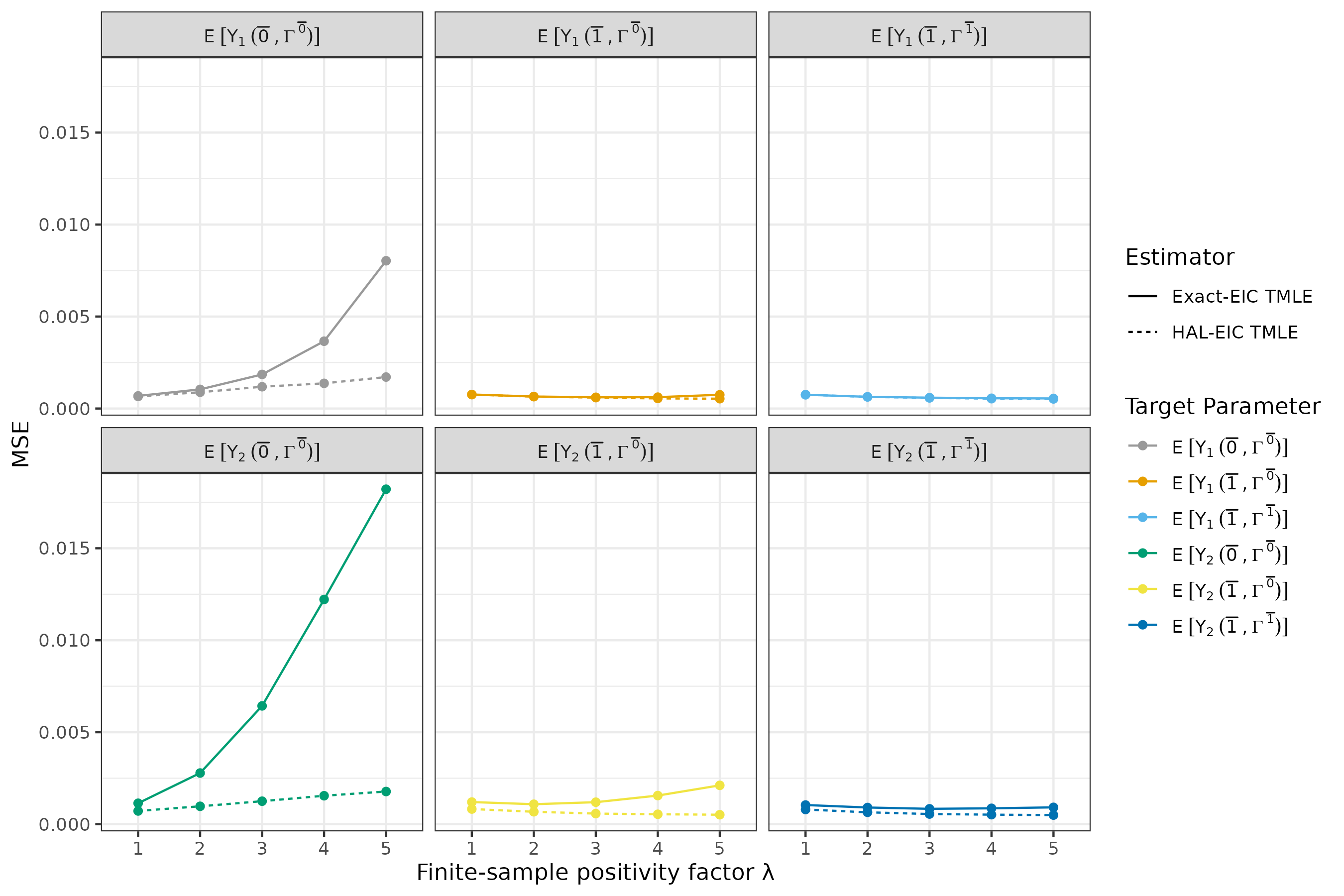
Figure 1: MSE comparison with increasing finite-sample positivity violation.

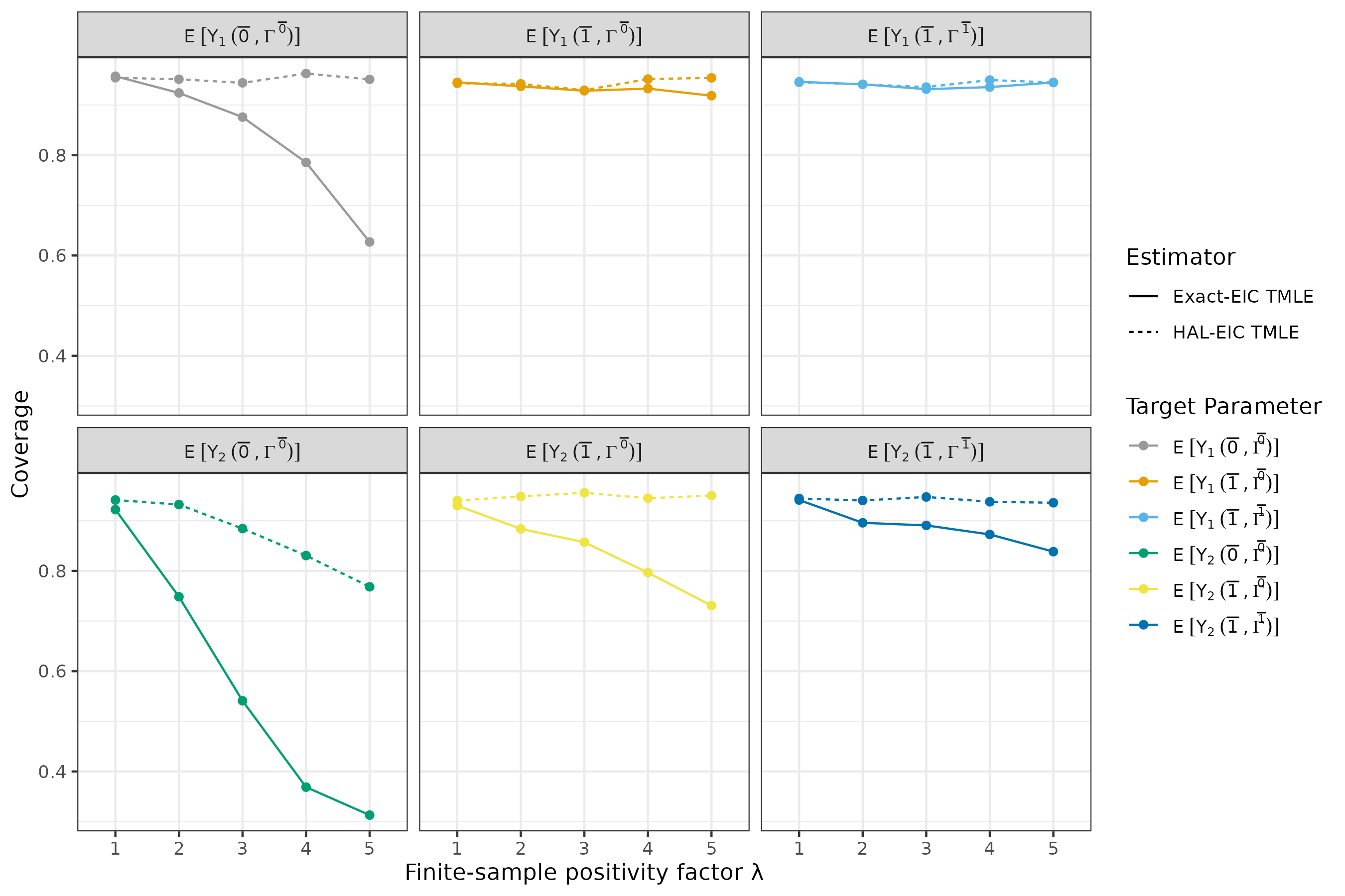
Figure 2: Coverage comparison with increasing finite-sample positivity violation.

9 Discussion

In this manuscript, we construct a scalable, likelihood and random intervention based estimation framework for longitudinal mediation. One advantage of our framework is its flexibility being a likelihood based method. This leads to an estimation procedure that is able to target multi-dimensional parameters simultaneously by updating estimators of the same estimate of the longitudinal likelihood process. Moreover, our HAL-EIC approximation further reduces the burden on practitioners, as the required input of the algorithms is reduced to modeling constraints of conditional distributions which is a well-known task for data scientists and can be implemented without further understanding of either the analytic calculation of the EIC or the sequential regression equations.

An important extension of our work is the application of collaborative TMLE (van der Laan and Gruber, 2010), which can be crucial in longitudinal problems where finite-sample positivity violations occur (Petersen et al., 2011). While the numerical HAL-EIC representation proposed in Section 6.1 implicitly searches for an optimal bound of the sectional variation norms on the EIC components and demonstrates robustness in the simulation, collaborative TMLE may be combined with the proposed estimators to achieve even more reliable inference. Previous results show that this is a promising direction to optimize the finite-sample performance (Ju, Schwab and van der Laan, 2019) .

Another idea that needs further work is a data adaptive choice of a dimension reduction algorithm for applications with high dimensional time-varying covariates. This can be conducted so that scalability is further improved while maintaining asymptotic properties for the estimators of the target parameters.

Future research should also consider generalize to continuous time TMLE (Rytgaard, Gerds and van der Laan, 2021) for applications where it is of interest to apply longitudinal mediation analysis to data structures where events are happening and are recorded in continuous time. Higher order TMLE (van der Laan, Wang and van der Laan, 2021) should be utilized to improve efficiency.

[Acknowledgments] This research is partially funded by NIH-grant R01AI074345-10A1. Additional funding was provided by a philanthropic gift from Novo Nordisk to the Center for Targeted Machine Learning and Causal Inference at UC Berkeley.

Appendix A Efficient Influence Curves (EIC)

To prove the EIC representation in Section 3.4, we utilize the pathwise differentiability of $\Psi^{\bar{a},\bar{a}^{\prime}}_{s}(P)$ and have that (suppressing its dependence on $\bar{a},\bar{a}^{\prime},s$, and let $Y=\psi_{s}(\bar{L}_{K})$)

$$\frac{\mathrm{d}\Psi(P_{\epsilon}^{h})}{\mathrm{d}\epsilon}_{|\epsilon=0}=\langle D(P),h\rangle_{P}$$

for all submodel $P^{h}_{\epsilon}$ through $P$, such that $h=\frac{\mathrm{d}}{\mathrm{d}\epsilon}_{|\epsilon=0}\log p^{h}_{\epsilon}$. Note that $h\in T(P)$ can be decomposed as $h=\sum_{X}h_{X}$ where $X\in\bar{L}\cup\bar{R}\cup\bar{Z}$, which corresponds to the factorization of the submodel

$$p^{h}_{\epsilon}=\prod_{X\in\bar{L}\cup\bar{R}\cup\bar{Z}}p^{h}_{\epsilon,X}=\prod_{X\in\bar{L}\cup\bar{R}\cup\bar{Z}}p_{X}(1+\epsilon h_{X}).$$

For all $h\in T(P)$ such that $h_{Z_{t}}=0$ for all $t=1,\dots,K$, we have that

$$\frac{\mathrm{d}\Psi(P_{\epsilon}^{h})}{\mathrm{d}\epsilon}_{|\epsilon=0}= \frac{\mathrm{d}\Psi(\prod_{t=1}^{K}p_{Z_{t}}\prod_{X\in\bar{L}\cup\bar{R}}p^{h}_{\epsilon,X})}{\mathrm{d}\epsilon}_{|\epsilon=0}$$

$$= \frac{\mathrm{d}\sum_{\bar{l},\bar{z},\bar{r}}y\prod_{X\in\bar{L}\cup\bar{R}}p^{h_{X}}_{\epsilon,X}(x|\text{Pa}(x|\bar{a})){\color[rgb]{1,0,0}\prod_{t=1}^{K}\mathbb{I}_{\left\{A_{t}=a_{t}\right\}}\prod_{t=1}^{K}p_{Z_{t}}(z_{t}|\text{Pa}(z_{t}|\bar{a}_{t}^{\prime}))}}{\mathrm{d}\epsilon}_{|\epsilon=0}$$

$$= \langle\sum_{X\in\bar{L}\cup\bar{R}}D_{X}(P),\sum_{X\in\bar{L}\cup\bar{R}}h_{X}\rangle_{P}$$

which corresponds to the pathwise derivative of the treatment specific mean under interventions $A_{t}=a_{t}$ and $Z_{t}\sim p_{Z_{t}}(Z_{t}|\text{Pa}(Z_{t}|\bar{a}^{\prime}))$. Apply $\Gamma_{t}(Z_{t}|\text{Pa}(Z_{t}))=p_{Z_{t}}(Z_{t}|\text{Pa}(Z_{t}|\bar{a}^{\prime}))$ in Lemma A.1. This gives the efficient influence function $\sum_{X\in\bar{L}\cup\bar{R}}D_{X}(P)$ as specified in Section 3.4.

On the other hand, to calculate $D_{Z_{t}}(P)$, consider $h\in T(P)$ such that $h_{X}=0$ for all $X\in\bar{L}\cup\bar{R}$. Then

$$\frac{\mathrm{d}\Psi(P_{\epsilon}^{h})}{\mathrm{d}\epsilon}_{|\epsilon=0}= \frac{\mathrm{d}\sum_{\bar{l},\bar{z},\bar{r}}y{\color[rgb]{1,0,0}\prod_{t=1}^{K}\mathbb{I}_{\left\{A_{t}=a_{t}^{\prime}\right\}}\prod_{X\in\bar{L}\cup\bar{R}}p_{X}(x|\text{Pa}(x|\bar{a}))}\prod_{t=1}^{K}p^{h_{Z_{t}}}_{\epsilon,Z_{t}}(z_{t}|\text{Pa}(z_{t}|\bar{a}_{t}^{\prime}))}{\mathrm{d}\epsilon}_{|\epsilon=0}$$

$$= \langle\sum_{t=1}^{K}D_{Z_{t}}(P),\sum_{t=1}^{K}h_{Z_{t}}\rangle_{P},$$

which corresponds to the pathwise derivative of the treatment specific mean under interventions $A_{t}=a_{t}^{\prime}$ and $X\sim p_{X}(X|\text{Pa}(X|\bar{a}))$ for all $X\in\bar{L}\cup\bar{R}$. This proves the rest of the EIC components $\sum_{t=1}^{K}D_{Z_{t}}(P)$ in Section 3.4.

Lastly, note that the orthogonal decomposition gives that $\langle D_{Z_{t}}(P),\sum_{X\in\bar{L}\cup\bar{R}}h_{X}\rangle_{P}=0$ and $\langle D_{R_{t}}(P)+D_{L_{t}}(P),\sum_{X\in\bar{Z}}h_{X}\rangle_{P}=0$. Therefore, $\frac{\mathrm{d}\Psi(P_{\epsilon}^{h})}{\mathrm{d}\epsilon}_{|\epsilon=0}=\langle\sum_{t=1}^{K}D_{Z_{t}}(P)+D_{R_{t}}(P)+D_{L_{t}}(P),h\rangle_{P}$ for all $h\in T(P)$. This proves that $D(P)=\sum_{X\in\bar{L}\cup\bar{R}\cup\bar{Z}}D_{X}(P)$ is the gradient and hence the unique canonical gradient in the nonparametric tangent space $T(P)$.

A.1 EIC of Other Longitudinal Interventions

Controlled direct effect (CDE)

Suppose that we replace the random intervention $Z_{t}(\bar{a},\bar{\Gamma}^{\bar{a}^{\prime}})\sim\Gamma^{\bar{a}^{\prime}}_{t}$ in 2.1 with enforcing a random draw $Z_{t}(\bar{a},\bar{\Gamma})\sim\Gamma_{t}$ that does not depend on the control group counterfactuals. A typical choice is letting $\Gamma_{t}$ be a degenerated discrete density function that puts probability $1$ to a certain value $z_{t}$, in which case the g-computation formula for $Y(\bar{a},\bar{\Gamma})$ is identical to that of $Y(\bar{a},\bar{z})$ following static intervention. Another example is when we believe that some estimator $\hat{\Gamma}_{t}$ is a satisfactory proxy for the unobserved $\bar{\Gamma}^{\bar{a}^{\prime}}$, and we focus on $Y(\bar{a},\bar{\Gamma}=\bar{\hat{\Gamma}})$ despite the caveat that interpretation may be limited when $\bar{\hat{\Gamma}}$ is too deviated from $\bar{\Gamma}^{\bar{a}^{\prime}}$. In general, these correspond to some joint intervention on $\bar{A}$ and $\bar{Z}$, where the (random/stochastic) CDE,

$$\mathbb{E}\left[Y(\bar{a},\bar{\Gamma})-Y(\bar{a}^{\prime},\bar{\Gamma})\right],$$

becomes a standard average treatment effect (ATE) parameter under random intervention of both $\bar{A}$ and $\bar{Z}$. For either $\Psi(P)=\mathbb{E}\left[Y(\bar{a},\bar{\Gamma})\right]$ or $\mathbb{E}\left[Y(\bar{a}^{\prime},\bar{\Gamma})\right]$, $p_{Z_{t}}$ becomes nuisance in the sense that any submodel $P^{h}_{\epsilon}$ with score $h\in T_{Z}(P)$ leads to $\frac{\mathrm{d}\Psi(P^{h}_{\epsilon})}{\mathrm{d}\epsilon}=0$. This leads to $D(P)\perp T_{Z}(P)$ and $D_{Z}(P)=0$. For $X\in\bar{L}\cup\bar{R}$, similar proof of EIC decomposition over $X\in\bar{L}\cup\bar{R}$ applies by replacing $Z_{t}\sim p_{Z_{t}}(Z_{t}|\text{Pa}(Z_{t}|\bar{a}^{\prime}))$ with $Z_{t}\sim\Gamma_{t}(Z_{t}|\text{Pa}(Z_{t}))$ (see Lemma A.1). The same methodology for NIE and NDE applies except that the EIC $D(P)$ now has $D_{Z_{t}}=0$ and that a known and fixed function, $\Gamma_{t}(Z_{t}|\text{Pa}(Z_{t}))$, replacing $p_{Z_{t}}(Z_{t}|\text{Pa}(Z_{t}|\bar{a}^{\prime}))$ in $D_{R_{t}}(P)$ and $D_{L_{t}}(P)$.

General longitudinal stochastic intervention

For the average treatment effect of a general longitudinal stochastic intervention (which could be a mixture of fixed and random interventions), suppose that $\bar{A}$ denotes the static intervention nodes and $\bar{Z}$ denotes the random intervention nodes onto the SCM in Section 2.1 . At the contrast of $(\bar{a},\bar{\Gamma}^{(1)})$ and $(\bar{a}^{\prime},\bar{\Gamma}^{(2)})$ with distinct $\bar{\Gamma}^{(1)}$ and $\bar{\Gamma}^{(2)}$, one can define the generalized ATE under this mixed intervention as

$$\mathbb{E}\left[Y(\bar{a},\bar{\Gamma}^{(1)})-Y(\bar{a}^{\prime},\bar{\Gamma}^{(2)})\right].$$

For $\bar{\Gamma}=\bar{\Gamma}^{(1)}$ or $\bar{\Gamma}^{(2)}$, we have the following lemma for the EIC of $\Psi(P)=\mathbb{E}\left[Y(\bar{a},\bar{\Gamma})\right]$.

Lemma A.1.

For $\bar{X}=\bar{R}$ or $\bar{L}$ and $\Psi(P)=\mathbb{E}\left[Y(\bar{a},\bar{\Gamma})\right]$ where $\bar{\Gamma}$ is a set of known density function for $\bar{Z}$ (in the sense that $\bar{Z}(O)$ is a fixed function of $O$), assume that $\mathbb{E}\left[Y(\bar{a},\bar{\Gamma})\right]$ is identified by the similar g-computation formula as Equation 2 but replacing $p_{Z}(Z_{t}|\text{Pa}(Z_{t}|\bar{a}^{\prime}))$ with $\Gamma_{t}(Z_{t}|\text{Pa}(Z_{t}))$. Define

$$Q_{R_{K+1}}^{\bar{a},\bar{\Gamma}}= Y$$

$$Q_{L_{t}}^{\bar{a},\bar{\Gamma}}\left(\bar{R}_{t},\bar{Z}_{t},\bar{L}_{t-1}\right)= \mathbb{E}_{P^{\bar{a},\bar{\Gamma}}}\left[Q_{R_{t+1}}^{\bar{a},\bar{\Gamma}}|\bar{R}_{t},\bar{Z}_{t},\bar{L}_{t-1}\right]=\mathbb{E}_{P}\left[Q_{R_{t+1}}^{\bar{a},\bar{\Gamma}}|\bar{R}_{t},\bar{Z}_{t},\bar{L}_{t-1},\bar{A}_{t}=\bar{a}_{t}\right]$$

$$Q_{Z_{t}}^{\bar{a},\bar{\Gamma}}\left(\bar{R}_{t},\bar{Z}_{t-1},\bar{L}_{t-1}\right)= \mathbb{E}_{P^{\bar{a},\bar{\Gamma}}}\left[Q_{L_{t}}^{\bar{a},\bar{\Gamma}}|\bar{R}_{t},\bar{Z}_{t-1},\bar{L}_{t-1}\right]=\sum_{z_{t}}Q_{L_{t}}^{\bar{a},\bar{\Gamma}}\Gamma_{t}(z_{t}|\text{Pa}(Z_{t}))$$

$$Q_{R_{t}}^{\bar{a},\bar{\Gamma}}\left(\bar{R}_{t-1},\bar{Z}_{t-1},\bar{L}_{t-1}\right)= \mathbb{E}_{P^{\bar{a},\bar{\Gamma}}}\left[Q_{Z_{t}}^{\bar{a},\bar{\Gamma}}|\bar{R}_{t-1},\bar{Z}_{t-1},\bar{L}_{t-1}\right]=\mathbb{E}_{P}\left[Q_{Z_{t}}^{\bar{a},\bar{\Gamma}}|\bar{R}_{t-1},\bar{Z}_{t-1},\bar{L}_{t-1},\bar{A}_{t}=\bar{a}_{t}\right]$$

$$\Psi^{\bar{a},\bar{\Gamma}}(P)= \mathbb{E}_{P}Q_{R_{1}}^{\bar{a},\bar{\Gamma}}(P)(L_{0}),$$

and

$$D^{\bar{a},\bar{\Gamma}}_{L_{t}}= \frac{\mathbb{I}_{\left\{\bar{A}_{t}=\bar{a}_{t}\right\}}}{\prod_{j=1}^{t}p_{A}(a_{j}|\text{Pa}(A_{j}|\bar{a}_{j-1}))}\prod_{j=1}^{t}\frac{\Gamma_{t}(Z_{j}|\text{Pa}(Z_{j}))}{p_{Z}(Z_{j}|\text{Pa}(Z_{j}|\bar{a}_{j}))}\left\{Q_{R_{t+1}}^{\bar{a},\bar{\Gamma}}(\bar{R}_{t},\bar{Z}_{t},\bar{L}_{t})-Q_{L_{t}}^{\bar{a},\bar{\Gamma}}(\bar{R}_{t},\bar{Z}_{t},\bar{L}_{t-1})\right\}$$

$$D^{\bar{a},\bar{\Gamma}}_{R_{t}}= \frac{\mathbb{I}_{\left\{\bar{A}_{t}=\bar{a}_{t}\right\}}}{\prod_{j=1}^{t}p_{A}(a_{j}|\text{Pa}(A_{j}|\bar{a}_{j-1}))}\prod_{j=1}^{t-1}\frac{\Gamma_{t}(Z_{j}|\text{Pa}(Z_{j}))}{p_{Z}(Z_{j}|\text{Pa}(Z_{j}|\bar{a}_{j}))}\left\{Q_{Z_{t}}^{\bar{a},\bar{\Gamma}}(\bar{R}_{t},\bar{Z}_{t-1},\bar{L}_{t-1})-Q_{R_{t}}^{\bar{a},\bar{\Gamma}}(\bar{R}_{t-1},\bar{Z}_{t-1},\bar{L}_{t-1})\right\}.$$

Then the EIC of $\Psi(P)$ is $D^{\bar{a},\bar{\Gamma}}(P)=\sum_{X_{t}\in\bar{R}\cup\bar{L}}D^{\bar{a},\bar{\Gamma}}_{X_{t}}(P)$.

Appendix B Projection Representation of EIC

For Lemma 6.1, recall that in Appendix A we proved that $\sum_{X\in\bar{R}\cup\bar{L}}D_{X}(P)$ is the influence curve of the treatment specific mean (TSM) under interventions $A_{t}=a_{t}$ and $Z_{t}\sim p_{Z_{t}}(Z_{t}|\text{Pa}(Z_{t}|\bar{a}^{\prime}))$. For such TSM parameter, an influence curve in the semiparametric model where $p_{A}$ and $p_{Z}$ are assumed known can be derived from the IPW estimator $\frac{1}{n}\sum_{t=1}^{K}\frac{Y\mathbb{I}_{\left\{\bar{A}=\bar{a}\right\}}}{\prod_{j=1}^{K}p_{A}(a_{j}|\text{Pa}(A_{j}|\bar{a}_{j-1}))}\cdot\frac{\prod_{j=1}^{K}p_{Z}(Z_{j}|\text{Pa}(Z_{j}|\bar{a}^{\prime}_{j}))}{\prod_{j=1}^{K}p_{Z}(Z_{j}|\text{Pa}(Z_{j}|\bar{a}_{j}))}$ (van der Laan, 2018). Then the influence function in the nonparametric model is the projection of this semiparametric influence curve onto the tangent space. Therefore, for $X\in\bar{R}\cup\bar{L}$,

$$D_{X}^{\bar{a},\bar{a}^{\prime}}(P)=\prod\left(\prod\left(G^{\bar{a},\bar{a}^{\prime}}_{LR}|L_{0}^{2}(P)\right)|T_{X}(P)\right)=\prod\left(G^{\bar{a},\bar{a}^{\prime}}_{LR}|T_{X}(P)\right),$$

where $L_{0}^{2}(P)$ is the collection of finite variance functions $f(O)$ such that $\mathbb{E}_{P}\left[f(O)\right]=0$. The same applies to $\sum_{X\in\bar{Z}}D_{X}(P)$ that is derived as the influence curve of the TSM under intervention $A_{t}=a_{t}^{\prime}$, $R_{t}\sim p_{R_{t}}(R_{t}|\text{Pa}(R_{t}|\bar{a}))$, and $L_{t}\sim p_{L_{t}}(L_{t}|\text{Pa}(L_{t}|\bar{a}))$.

Lemma 6.1 can also be verified with algebraic calculation using $\prod\left(f|T_{X}(P)\right)=\mathbb{E}_{P}\left[f|X,\text{Pa}(X)\right]-\mathbb{E}_{P}\left[f|\text{Pa}(X)\right]$ and expanding the integral terms of conditional expectations.

Appendix C Centered HAL Basis

Suppose that $D_{X}^{*}(P)$ is one of the EIC component listed in Section 3.4 associated with the tangent space $T_{X}(P)=\left\{h(X|\text{Pa}(X)):\mathbb{E}_{P}\left\{h(X|\text{Pa}(X))|\text{Pa}(X)\right\})=0\right\}$. In this section, we present an alternative representation of $D_{X}^{*}(P)$ as a linear combination of centered HAL basis functions, and the TMLE updates based on the approximation.

If we have an initial gradient $G_{X}(P)$ such that its projection onto the tangent space $\prod\left(G_{X}(P)|T_{X}(P)\right)$ equals the EIC component $D^{*}_{X}(P)$ (Lemma 6.1 as an example), and if $T_{X}(P)$ is well approximated by the linear span of a set of basis functions $\{\phi_{j,X}(P):j\}$, then we can have the following EIC representation

$$D^{*}_{X}(P)=\sum_{j}\beta_{j,X}(P)\phi_{j,X}(P),$$

where the coefficients $\beta_{X}(P)=(\beta_{j,X}(P):j)$ are defined by the least squared projection

$$\beta_{X}(P)=\arg\min_{\beta}P\left\{G_{X}(P)-\sum_{j}\beta_{j}\phi_{j,X}(P)\right\}^{2}.$$

In practice, a large sample of size $N$ can be generated from $P$, and a follow-up cross-validated lasso regression against a subset of $\{\phi_{j,X}(P):j\}$ of size $J$ will decide at most $N-1$ non-zero coefficients in the following approximated representation with a finite sectional variation norm

$$\hat{D}^{*}_{X}(P)=\sum_{j=1}^{J}\hat{\beta}_{j,X}(P)\phi_{j,X}(P).$$

Under assumption (B4), $T_{X}(P)$ is a subspace of the space of cadlag functions of $(X,\text{Pa}(X))$ with bounded sectional variation norms, where the latter is the space spanned by the (uncentered) HAL basis in the following form (see Section 6.2 of van der Laan et al. (2018)):

$$\phi_{j,X}=\mathbb{I}_{\left\{U(X)\geq\mu_{j}\right\}},$$

where $U(X)=(X,\text{Pa}(X))$. $u_{j}$ is a knot point in the range of a subvector of $U(X)$, where each element of $u_{j}$ takes a value in $\mathbb{R}\cup\left\{-\infty\right\}$. Conducting the projection onto $T_{X}(P)$ in two steps gives

$${D}^{*}_{X}(P)=\sum_{j}\beta_{j,X}(P)\phi_{j,X}(P),$$

where $\phi_{j,X}(P)=\Pi(\phi_{j,X}|T_{X}(P))=\phi_{j,X}-\mathbb{E}_{P}\left[\phi_{j,X}|\text{Pa}(X)\right]=\mathbb{I}_{\left\{\text{Pa}(X)\geq\text{Pa}(x)(\mu_{j})\right\}}\left(\mathbb{I}_{\left\{X\geq x(\mu_{j})\right\}}-P(X\geq x(\mu_{j})|\text{Pa}(X))\right).$ By the construction of finite-sample HAL estimator (van der Laan et al., 2018), using the regenerated IID sample following $P$ of size $N$, a finite subset of $\left\{\phi_{j,X}(P):j\right\}$ of size $J$ can be chosen such that the corresponding cross-validated lasso estimator $\hat{D}^{*}_{X}(P)=\sum_{j}^{J}\hat{\beta}_{j,X}(P)\phi_{j,X}(P)$ satisfies the convergence rate $\left\lVert\hat{D}^{*}_{X}(P)-D^{*}_{X}(P)\right\rVert_{P}=O_{P}(N^{-1/3}(\log N)^{d/2})$.

Appendix D HAL-EIC TMLE

Note that there is only one additional term imposed to the expansion (4),

$$P_{n}\left\{\boldsymbol{D}^{F}(P_{n}^{*})-\hat{\boldsymbol{D}}^{F}(P_{n}^{*})\right\}$$

$$= (P_{n}-P_{0})\left\{{\boldsymbol{D}}^{F}(P_{n}^{*})-\hat{\boldsymbol{D}}^{F}(P_{n}^{*})\right\}+(P_{0}-P_{n}^{*})\left\{{\boldsymbol{D}}^{F}(P_{n}^{*})-\hat{\boldsymbol{D}}^{F}(P_{n}^{*})\right\}.$$

To maintain the asymptotic efficiency achieved under the assumptions listed in Section 5.3, 1) the first part converges under the similar Donsker condition, and 2) with the known HAL error rate (Bibaut and van der Laan, 2019) of $\left\lVert D^{*}_{X}(P)-\hat{D}^{*}_{X}(P)\right\rVert_{P}=O_{P}(N^{-1/3}(\log N)^{d/2})$ where $\left\lVert g(O)\right\rVert_{P}=\sqrt{\langle g,g\rangle_{P}}=\sqrt{Pg^{2}}=\sqrt{\int g(o)^{2}p(o)d\mu}$ is the $L^{2}(P)$ norm, the second part (assuming the $L^{2}(\mu)$ norm below is applied element-wise for vectors) by the Cauchy Schwarz inequality

$$\left\lVert(P_{0}-P_{n}^{*})\left\{{\boldsymbol{D}}^{F}(P_{n}^{*})-\hat{\boldsymbol{D}}^{F}(P_{n}^{*})\right\}\right\rVert\leq \left\lVert\left\lVert p_{0}-p_{n}^{*}\right\rVert_{\mu}\cdot\left\lVert{\boldsymbol{D}}^{F}(P_{n}^{*})-\hat{\boldsymbol{D}}^{F}(P_{n}^{*})\right\rVert_{\mu}\right\rVert,$$

only requires (B5), that is, either $\left\lVert p_{0}-p_{n}^{*}\right\rVert_{P_{0}}=o_{P}(n^{-1/6})$ when we select $N=n$, or requires no additional condition when $N(n)$ increases at a faster rate than $n^{3/2}$, under the assumptions that $p_{0}(o)>\delta>0$ and $p_{n}^{*}(o)>\delta>0$ over the supports for some $\delta>0$.

In practice, we can simulate with $N>n$ to further improve the finite sample performance, and HAL can be included as one of the estimators in the super learner for $P_{n}^{0}$ so that $\left\lVert p_{0}-p_{n}^{*}\right\rVert_{P_{0}}=O_{P}(n^{-1/3}(\log n)^{d/2})$ is guaranteed.

Appendix E Multiple Robustness and Exact Remainders

First, focus on one of the dimensions $\Psi(P)=\Psi^{\bar{a},\bar{a}^{\prime}}_{s}(P)$ and its corresponding exact remainder as $R(P,P_{0})=R^{\bar{a},\bar{a}^{\prime}}_{s}(P,P_{0})$. Then by definition of Section 5.3,

$$R(P,P_{0}) =\Psi(P)-\Psi(P_{0})+P_{0}D(P)$$

$$=PQ_{R_{1}}(P)-P_{0}Q_{R_{1}}(P_{0})+\sum_{X\in\bar{R}\cup\bar{Z}\cup\bar{L}}P_{0}D_{X}(P)$$

Define the following generalized propensity terms:

$$\pi^{k}_{A}= \prod_{t=1}^{k}p_{A}(A_{t}|\text{Pa}(A_{t})),~{}\pi^{k}_{0,A}=\prod_{t=1}^{k}p_{0,A}(A_{t}|\text{Pa}(A_{t}))$$

$$\pi^{k}_{R}= \prod_{t=1}^{k}p_{R}(R_{t}|\text{Pa}(R_{t})),~{}\pi^{k}_{0,R}=\prod_{t=1}^{k}p_{0,R}(R_{t}|\text{Pa}(R_{t}))$$

$$\pi^{k}_{Z}= \prod_{t=1}^{k}p_{Z}(Z_{t}|\text{Pa}(Z_{t})),~{}\pi^{k}_{0,Z}=\prod_{t=1}^{k}p_{0,Z}(Z_{t}|\text{Pa}(Z_{t}))$$

$$\pi^{k}_{L}= \prod_{t=1}^{k}p_{L}(L_{t}|\text{Pa}(L_{t})),~{}\pi^{k}_{0,L}=\prod_{t=1}^{k}p_{0,L}(L_{t}|\text{Pa}(L_{t}))$$

$$\pi^{*k,\bar{a}}_{A}= \prod_{t=1}^{k}\mathbb{I}_{\left\{A_{t}=a_{t}\right\}}$$

$$\pi^{*k,\bar{a}^{\prime}}_{A}= \prod_{t=1}^{k}\mathbb{I}_{\left\{A_{t}=a_{t}^{\prime}\right\}}$$

$$\pi^{*k}_{R}= \prod_{t=1}^{k}p_{R}(R_{t}|\text{Pa}(R_{t}|\bar{a}_{t})),~{}\pi^{*k}_{0,R}=\prod_{t=1}^{k}p_{0,R}(R_{t}|\text{Pa}(R_{t}|\bar{a}_{t}))$$

$$\pi^{*k}_{Z}= \prod_{t=1}^{k}p_{Z}(Z_{t}|\text{Pa}(Z_{t}|\bar{a}_{t}^{\prime})),~{}\pi^{*k}_{0,Z}=\prod_{t=1}^{k}p_{0,Z}(Z_{t}|\text{Pa}(Z_{t}|\bar{a}_{t}^{\prime}))$$

$$\pi^{*k}_{L}= \prod_{t=1}^{k}p_{L}(L_{t}|\text{Pa}(L_{t}|\bar{a}_{t})),~{}\pi^{*k}_{0,L}=\prod_{t=1}^{k}p_{0,L}(L_{t}|\text{Pa}(L_{t}|\bar{a}_{t})),$$

then

$$D_{L_{t}}(P)= \frac{\pi^{*t,\bar{a}}_{A}\pi^{*t}_{Z}}{\pi^{t}_{A}\pi^{t}_{Z}}(Q_{R_{t+1}}-Q_{L_{t}})$$

$$D_{Z_{t}}(P)= \frac{\pi^{*t,\bar{a}^{\prime}}_{A}\pi^{*t}_{R}\pi^{*,t-1}_{L}}{\pi^{t}_{A}\pi^{t}_{R}\pi^{t-1}_{L}}(Q_{L_{t}}-Q_{Z_{t}})$$

$$D_{R_{t}}(P)= \frac{\pi^{*t,\bar{a}}_{A}\pi^{*,t-1}_{Z}}{\pi^{t}_{A}\pi^{t-1}_{Z}}(Q_{Z_{t}}-Q_{R_{t}}).$$

Plug in to the exact remainder above (let $Q_{X}=Q_{X}(P)$ when the dependence is not specified), and note that

$$P_{0}Q_{R_{1}}(P_{0})= P_{0}G_{L}(P_{0})=P_{0}\frac{\pi^{*K,\bar{a}}_{A}\pi^{*K}_{0,Z}}{\pi^{K}_{0,A}\pi^{K}_{0,Z}}Y$$

$$P_{0}D_{R_{1}}(P)= P_{0}(Q_{Z_{1}}(P)-Q_{R_{1}}(P))$$

$$P_{0}Q_{R_{1}}(P_{0})-P_{0}Q_{R_{1}}(P)= P_{0}\frac{\pi^{*K,\bar{a}}_{A}\pi^{*K}_{0,Z}}{\pi^{K}_{0,A}\pi^{K}_{0,Z}}(Y-Q_{L_{K}}(P))+P_{0}\frac{\pi^{*K,\bar{a}^{\prime}}_{A}\pi^{*K}_{0,R}\pi^{*,K-1}_{0,L}}{\pi^{K}_{0,A}\pi^{K}_{0,R}\pi^{K-1}_{0,L}}(Q_{L_{K}}(P)-Q_{Z_{K}}(P))+\cdots$$

$$+P_{0}(Q_{Z_{1}}(P)-Q_{R_{1}}(P)),$$

and therefore (still let $Q_{X}=Q_{X}(P)$ for clarity)

$$R(P,P_{0})= -P_{0}Q_{R_{1}}(P_{0})+P_{0}Q_{R_{1}}(P)+$$

$$\sum_{t=1}^{K}\left(P_{0}\frac{\pi^{*t,\bar{a}}_{A}\pi^{*t}_{Z}}{\pi^{t}_{A}\pi^{t}_{Z}}(Q_{R_{t+1}}-Q_{L_{t}})+P_{0}\frac{\pi^{*t,\bar{a}^{\prime}}_{A}\pi^{*t}_{R}\pi^{*,t-1}_{L}}{\pi^{t}_{A}\pi^{t}_{R}\pi^{t-1}_{L}}(Q_{L_{t}}-Q_{Z_{t}})+P_{0}\frac{\pi^{*t,\bar{a}}_{A}\pi^{*,t-1}_{Z}}{\pi^{t}_{A}\pi^{t-1}_{Z}}(Q_{Z_{t}}-Q_{R_{t}})\right)$$

$$= \sum_{t=1}^{K}\Bigg{(}P_{0}(\frac{\pi^{*t,\bar{a}}_{A}\pi^{*t}_{Z}}{\pi^{t}_{A}\pi^{t}_{Z}}-\frac{\pi^{*t,\bar{a}}_{A}\pi^{*t}_{0,Z}}{\pi^{t}_{0,A}\pi^{t}_{0,Z}})(Q_{R_{t+1}}-Q_{L_{t}})+$$

$$P_{0}(\frac{\pi^{*t,\bar{a}^{\prime}}_{A}\pi^{*t}_{R}\pi^{*,t-1}_{L}}{\pi^{t}_{A}\pi^{t}_{R}\pi^{t-1}_{L}}-\frac{\pi^{*t,\bar{a}^{\prime}}_{A}\pi^{*t}_{0,R}\pi^{*,t-1}_{0,L}}{\pi^{t}_{0,A}\pi^{t}_{0,R}\pi^{t-1}_{0,L}})(Q_{L_{t}}-Q_{Z_{t}})+$$

$$P_{0}(\frac{\pi^{*t,\bar{a}}_{A}\pi^{*,t-1}_{0,Z}}{\pi^{t}_{A}\pi^{t-1}_{Z}}-\frac{\pi^{*t,\bar{a}}_{A}\pi^{*,t-1}_{Z}}{\pi^{t}_{0,A}\pi^{t-1}_{0,Z}})(Q_{Z_{t}}-Q_{R_{t}})\Bigg{)}.$$

Due to the sequential definition of $\left\{Q_{X}:X\in\bar{R},\bar{Z},\bar{L}\right\}$ as functions of $(p_{R},p_{Z},p_{L})$, one can check that $p_{R_{t}}=p_{0,R_{t}}$ leads to $P_{0}\left\{Q_{Z_{t}}-Q_{R_{t}}\right\}=0$, $p_{Z_{t}}=p_{0,Z_{t}}$ leads to $P_{0}\left\{Q_{L_{t}}-Q_{Z_{t}}\right\}=0$, and $p_{L_{t}}=p_{0,L_{t}}$ leads to $P_{0}\left\{Q_{R_{t+1}}-Q_{L_{t}}\right\}=0$. Under positivity assumptions, this proves the statement that under one of the following three scenarios we have $R(P,P_{0})=0$: 1) $p_{A}=p_{0,A}$ and $p_{Z}=p_{0,Z}$, 2) $p_{A}=p_{0,A}$ and $p_{R}=p_{0,R},p_{L}=p_{0,L}$, or 3) $p_{Z}=p_{0,Z}$ and $p_{R}=p_{0,R},p_{L}=p_{0,L}$.

Furthermore, under strong positivity and bounded variation norm assumptions as specified in (B4) and (B5), Cauchy-Schwarz inequality applies such that the aforementioned conditions are relaxed such that only $\left\lVert p_{X}-p_{0,X}\right\rVert_{P}=o_{P}(n^{-1/4})$ is required for 1) $X\in\bar{A}\cup\bar{Z}$, 2) $X\in\bar{A}\cup\bar{R}\cup\bar{L}$, or 3) $X\in\bar{Z}\cup\bar{R}\cup\bar{L}$. This proves the multiple robustness statement in Section 7.

Appendix F Numerical Results

$\mathbb{E}[Y_{1}(\bar{1},\Gamma^{\bar{1}})]$	Bias	SD	MSE	Coverage	Width
Exact-EIC Initial	0.0001	0.0274	0.0008	0.9465	0.1064
HAL-EIC Initial	0.0001	0.0274	0.0008	0.9455	0.1060
Exact-EIC TMLE	0.0000	0.0274	0.0008	0.9465	0.1064
HAL-EIC TMLE	0.0001	0.0274	0.0008	0.9455	0.1060
$\mathbb{E}[Y_{2}(\bar{1},\Gamma^{\bar{1}})]$	Bias	SD	MSE	Coverage	Width
Exact-EIC Initial	0.0003	0.0282	0.0008	0.9687	0.1259
HAL-EIC Initial	0.0004	0.0283	0.0008	0.9444	0.1085
Exact-EIC TMLE	0.0005	0.0323	0.0010	0.9414	0.1251
HAL-EIC TMLE	0.0004	0.0283	0.0008	0.9444	0.1085
$\mathbb{E}[Y_{1}(\bar{1},\Gamma^{\bar{0}})]$	Bias	SD	MSE	Coverage	Width
Exact-EIC Initial	0.0001	0.0275	0.0008	0.9455	0.1086
HAL-EIC Initial	0.0000	0.0275	0.0008	0.9434	0.1070
Exact-EIC TMLE	-0.0001	0.0276	0.0008	0.9455	0.1085
HAL-EIC TMLE	0.0000	0.0275	0.0008	0.9434	0.1070
$\mathbb{E}[Y_{2}(\bar{1},\Gamma^{\bar{0}})]$	Bias	SD	MSE	Coverage	Width
Exact-EIC Initial	0.0003	0.0287	0.0008	0.9737	0.1327
HAL-EIC Initial	0.0003	0.0287	0.0008	0.9404	0.1108
Exact-EIC TMLE	0.0002	0.0347	0.0012	0.9303	0.1306
HAL-EIC TMLE	0.0003	0.0287	0.0008	0.9404	0.1108
$\mathbb{E}[Y_{1}(\bar{0},\Gamma^{\bar{0}})]$	Bias	SD	MSE	Coverage	Width
Exact-EIC Initial	0.0021	0.0255	0.0007	0.9606	0.1056
HAL-EIC Initial	0.0021	0.0255	0.0007	0.9545	0.1031
Exact-EIC TMLE	0.0020	0.0261	0.0007	0.9576	0.1055
HAL-EIC TMLE	0.0021	0.0255	0.0007	0.9545	0.1031
$\mathbb{E}[Y_{2}(\bar{0},\Gamma^{\bar{0}})]$	Bias	SD	MSE	Coverage	Width
Exact-EIC Initial	-0.0006	0.0267	0.0007	0.9808	0.1290
HAL-EIC Initial	-0.0006	0.0268	0.0007	0.9414	0.1051
Exact-EIC TMLE	-0.0005	0.0338	0.0011	0.9222	0.1266
HAL-EIC TMLE	-0.0006	0.0268	0.0007	0.9414	0.1051

Table 1: Misspecification: none.

$\mathbb{E}[Y_{1}(\bar{1},\Gamma^{\bar{1}})]$	Bias	SD	MSE	Coverage	Width
Exact-EIC Initial	0.0002	0.0274	0.0008	0.8983	0.0894
HAL-EIC Initial	0.0002	0.0275	0.0008	0.9003	0.0889
Exact-EIC TMLE	0.0002	0.0274	0.0008	0.9003	0.0894
HAL-EIC TMLE	0.0002	0.0275	0.0008	0.9003	0.0889
$\mathbb{E}[Y_{2}(\bar{1},\Gamma^{\bar{1}})]$	Bias	SD	MSE	Coverage	Width
Exact-EIC Initial	0.0004	0.0284	0.0008	0.8983	0.0940
HAL-EIC Initial	0.0003	0.0284	0.0008	0.8602	0.0865
Exact-EIC TMLE	0.0007	0.0318	0.0010	0.8592	0.0937
HAL-EIC TMLE	0.0003	0.0284	0.0008	0.8602	0.0865
$\mathbb{E}[Y_{1}(\bar{1},\Gamma^{\bar{0}})]$	Bias	SD	MSE	Coverage	Width
Exact-EIC Initial	0.0001	0.0275	0.0008	0.9075	0.0914
HAL-EIC Initial	0.0002	0.0276	0.0008	0.9034	0.0903
Exact-EIC TMLE	0.0000	0.0277	0.0008	0.9096	0.0913
HAL-EIC TMLE	0.0002	0.0276	0.0008	0.9034	0.0903
$\mathbb{E}[Y_{2}(\bar{1},\Gamma^{\bar{0}})]$	Bias	SD	MSE	Coverage	Width
Exact-EIC Initial	0.0003	0.0289	0.0008	0.9013	0.0990
HAL-EIC Initial	0.0003	0.0289	0.0008	0.8654	0.0890
Exact-EIC TMLE	0.0004	0.0333	0.0011	0.8602	0.0983
HAL-EIC TMLE	0.0003	0.0289	0.0008	0.8654	0.0890
$\mathbb{E}[Y_{1}(\bar{0},\Gamma^{\bar{0}})]$	Bias	SD	MSE	Coverage	Width
Exact-EIC Initial	0.0021	0.0255	0.0007	0.9609	0.1048
HAL-EIC Initial	0.0022	0.0255	0.0007	0.9579	0.1043
Exact-EIC TMLE	0.0021	0.0255	0.0007	0.9568	0.1048
HAL-EIC TMLE	0.0022	0.0255	0.0007	0.9579	0.1043
$\mathbb{E}[Y_{2}(\bar{0},\Gamma^{\bar{0}})]$	Bias	SD	MSE	Coverage	Width
Exact-EIC Initial	-0.0005	0.0268	0.0007	0.9712	0.1187
HAL-EIC Initial	-0.0004	0.0269	0.0007	0.9353	0.1012
Exact-EIC TMLE	-0.0001	0.0298	0.0009	0.9466	0.1185
HAL-EIC TMLE	-0.0004	0.0269	0.0007	0.9353	0.1012

Table 2: Misspecification: A.

$\mathbb{E}[Y_{1}(\bar{1},\Gamma^{\bar{1}})]$	Bias	SD	MSE	Coverage	Width
Exact-EIC Initial	-0.0000	0.0274	0.0007	0.9477	0.1064
HAL-EIC Initial	0.0001	0.0274	0.0008	0.9443	0.1061
Exact-EIC TMLE	0.0001	0.0274	0.0007	0.9477	0.1064
HAL-EIC TMLE	0.0002	0.0274	0.0008	0.9455	0.1061
$\mathbb{E}[Y_{2}(\bar{1},\Gamma^{\bar{1}})]$	Bias	SD	MSE	Coverage	Width
Exact-EIC Initial	0.0003	0.0287	0.0008	0.9682	0.1260
HAL-EIC Initial	0.0003	0.0287	0.0008	0.9318	0.1087
Exact-EIC TMLE	0.0007	0.0329	0.0011	0.9364	0.1253
HAL-EIC TMLE	0.0005	0.0287	0.0008	0.9352	0.1086
$\mathbb{E}[Y_{1}(\bar{1},\Gamma^{\bar{0}})]$	Bias	SD	MSE	Coverage	Width
Exact-EIC Initial	0.0016	0.0274	0.0008	0.9511	0.1065
HAL-EIC Initial	0.0017	0.0274	0.0008	0.9455	0.1062
Exact-EIC TMLE	0.0002	0.0277	0.0008	0.9455	0.1068
HAL-EIC TMLE	0.0008	0.0274	0.0008	0.9420	0.1062
$\mathbb{E}[Y_{2}(\bar{1},\Gamma^{\bar{0}})]$	Bias	SD	MSE	Coverage	Width
Exact-EIC Initial	0.0017	0.0287	0.0008	0.9693	0.1261
HAL-EIC Initial	0.0017	0.0287	0.0008	0.9341	0.1094
Exact-EIC TMLE	-0.0000	0.0345	0.0012	0.9273	0.1263
HAL-EIC TMLE	0.0008	0.0290	0.0008	0.9284	0.1094
$\mathbb{E}[Y_{1}(\bar{0},\Gamma^{\bar{0}})]$	Bias	SD	MSE	Coverage	Width
Exact-EIC Initial	0.0041	0.0257	0.0007	0.9568	0.1055
HAL-EIC Initial	0.0041	0.0258	0.0007	0.9534	0.1031
Exact-EIC TMLE	0.0029	0.0261	0.0007	0.9580	0.1055
HAL-EIC TMLE	0.0031	0.0255	0.0007	0.9591	0.1031
$\mathbb{E}[Y_{2}(\bar{0},\Gamma^{\bar{0}})]$	Bias	SD	MSE	Coverage	Width
Exact-EIC Initial	0.0016	0.0277	0.0008	0.9773	0.1291
HAL-EIC Initial	0.0016	0.0278	0.0008	0.9352	0.1048
Exact-EIC TMLE	0.0006	0.0342	0.0012	0.9136	0.1268
HAL-EIC TMLE	0.0006	0.0273	0.0007	0.9455	0.1048

Table 3: Misspecification: Z.

$\mathbb{E}[Y_{1}(\bar{1},\Gamma^{\bar{1}})]$	Bias	SD	MSE	Coverage	Width
Exact-EIC Initial	0.0532	0.0186	0.0032	0.5111	0.1072
HAL-EIC Initial	0.0533	0.0188	0.0032	0.5069	0.1070
Exact-EIC TMLE	0.0003	0.0273	0.0007	0.9504	0.1068
HAL-EIC TMLE	0.0001	0.0276	0.0008	0.9409	0.1063
$\mathbb{E}[Y_{2}(\bar{1},\Gamma^{\bar{1}})]$	Bias	SD	MSE	Coverage	Width
Exact-EIC Initial	0.0494	0.0183	0.0028	0.8110	0.1281
HAL-EIC Initial	0.0494	0.0183	0.0028	0.6473	0.1105
Exact-EIC TMLE	0.0005	0.0320	0.0010	0.9525	0.1263
HAL-EIC TMLE	-0.0005	0.0279	0.0008	0.9472	0.1118
$\mathbb{E}[Y_{1}(\bar{1},\Gamma^{\bar{0}})]$	Bias	SD	MSE	Coverage	Width
Exact-EIC Initial	0.0549	0.0186	0.0034	0.4984	0.1096
HAL-EIC Initial	0.0549	0.0187	0.0034	0.4794	0.1082
Exact-EIC TMLE	0.0005	0.0276	0.0008	0.9493	0.1090
HAL-EIC TMLE	0.0009	0.0278	0.0008	0.9440	0.1074
$\mathbb{E}[Y_{2}(\bar{1},\Gamma^{\bar{0}})]$	Bias	SD	MSE	Coverage	Width
Exact-EIC Initial	0.0508	0.0183	0.0029	0.8332	0.1354
HAL-EIC Initial	0.0508	0.0183	0.0029	0.6547	0.1134
Exact-EIC TMLE	0.0002	0.0342	0.0012	0.9356	0.1319
HAL-EIC TMLE	-0.0001	0.0283	0.0008	0.9535	0.1147
$\mathbb{E}[Y_{1}(\bar{0},\Gamma^{\bar{0}})]$	Bias	SD	MSE	Coverage	Width
Exact-EIC Initial	0.0590	0.0186	0.0038	0.3749	0.1067
HAL-EIC Initial	0.0590	0.0188	0.0038	0.3601	0.1045
Exact-EIC TMLE	0.0021	0.0260	0.0007	0.9599	0.1057
HAL-EIC TMLE	0.0020	0.0255	0.0007	0.9588	0.1037
$\mathbb{E}[Y_{2}(\bar{0},\Gamma^{\bar{0}})]$	Bias	SD	MSE	Coverage	Width
Exact-EIC Initial	0.0536	0.0183	0.0032	0.7635	0.1330
HAL-EIC Initial	0.0537	0.0184	0.0032	0.5586	0.1105
Exact-EIC TMLE	-0.0005	0.0342	0.0012	0.9166	0.1277
HAL-EIC TMLE	-0.0002	0.0271	0.0007	0.9599	0.1119

Table 4: Misspecification: Y.

$\mathbb{E}[Y_{1}(\bar{1},\Gamma^{\bar{1}})]$	Bias	SD	MSE	Coverage	Width
Exact-EIC Initial	-0.0000	0.0251	0.0006	0.9394	0.0988
HAL-EIC Initial	-0.0001	0.0251	0.0006	0.9414	0.0978
Exact-EIC TMLE	-0.0001	0.0252	0.0006	0.9455	0.0988
HAL-EIC TMLE	-0.0001	0.0251	0.0006	0.9414	0.0978
$\mathbb{E}[Y_{2}(\bar{1},\Gamma^{\bar{1}})]$	Bias	SD	MSE	Coverage	Width
Exact-EIC Initial	-0.0001	0.0254	0.0006	0.9697	0.1142
HAL-EIC Initial	-0.0002	0.0254	0.0006	0.9404	0.0988
Exact-EIC TMLE	0.0004	0.0301	0.0009	0.9273	0.1129
HAL-EIC TMLE	-0.0002	0.0254	0.0006	0.9404	0.0988
$\mathbb{E}[Y_{1}(\bar{1},\Gamma^{\bar{0}})]$	Bias	SD	MSE	Coverage	Width
Exact-EIC Initial	0.0001	0.0254	0.0006	0.9424	0.1010
HAL-EIC Initial	0.0001	0.0254	0.0006	0.9424	0.0990
Exact-EIC TMLE	-0.0000	0.0256	0.0007	0.9414	0.1009
HAL-EIC TMLE	0.0001	0.0254	0.0006	0.9424	0.0990
$\mathbb{E}[Y_{2}(\bar{1},\Gamma^{\bar{0}})]$	Bias	SD	MSE	Coverage	Width
Exact-EIC Initial	-0.0000	0.0260	0.0007	0.9768	0.1209
HAL-EIC Initial	-0.0000	0.0260	0.0007	0.9485	0.1036
Exact-EIC TMLE	0.0006	0.0330	0.0011	0.9253	0.1185
HAL-EIC TMLE	-0.0000	0.0260	0.0007	0.9485	0.1036
$\mathbb{E}[Y_{1}(\bar{0},\Gamma^{\bar{0}})]$	Bias	SD	MSE	Coverage	Width
Exact-EIC Initial	0.0032	0.0296	0.0009	0.9677	0.1274
HAL-EIC Initial	0.0032	0.0296	0.0009	0.9515	0.1171
Exact-EIC TMLE	0.0035	0.0321	0.0010	0.9475	0.1270
HAL-EIC TMLE	0.0032	0.0296	0.0009	0.9515	0.1171
$\mathbb{E}[Y_{2}(\bar{0},\Gamma^{\bar{0}})]$	Bias	SD	MSE	Coverage	Width
Exact-EIC Initial	0.0007	0.0312	0.0010	0.9869	0.1896
HAL-EIC Initial	0.0008	0.0312	0.0010	0.9323	0.1227
Exact-EIC TMLE	0.0004	0.0528	0.0028	0.7869	0.1613
HAL-EIC TMLE	0.0008	0.0312	0.0010	0.9323	0.1227

Table 5: Misspecification: none, positivity scaling factor $\lambda=2$.

$\mathbb{E}[Y_{1}(\bar{1},\Gamma^{\bar{1}})]$	Bias	SD	MSE	Coverage	Width
Exact-EIC Initial	0.0010	0.0239	0.0006	0.9391	0.0948
HAL-EIC Initial	0.0012	0.0240	0.0006	0.9359	0.0930
Exact-EIC TMLE	0.0008	0.0243	0.0006	0.9391	0.0948
HAL-EIC TMLE	0.0012	0.0240	0.0006	0.9359	0.0930
$\mathbb{E}[Y_{2}(\bar{1},\Gamma^{\bar{1}})]$	Bias	SD	MSE	Coverage	Width
Exact-EIC Initial	0.0012	0.0235	0.0006	0.9695	0.1100
HAL-EIC Initial	0.0013	0.0235	0.0006	0.9475	0.0931
Exact-EIC TMLE	0.0015	0.0289	0.0008	0.9233	0.1077
HAL-EIC TMLE	0.0013	0.0235	0.0006	0.9475	0.0931
$\mathbb{E}[Y_{1}(\bar{1},\Gamma^{\bar{0}})]$	Bias	SD	MSE	Coverage	Width
Exact-EIC Initial	0.0011	0.0242	0.0006	0.9370	0.0970
HAL-EIC Initial	0.0013	0.0243	0.0006	0.9296	0.0947
Exact-EIC TMLE	0.0007	0.0247	0.0006	0.9370	0.0971
HAL-EIC TMLE	0.0013	0.0243	0.0006	0.9296	0.0947
$\mathbb{E}[Y_{2}(\bar{1},\Gamma^{\bar{0}})]$	Bias	SD	MSE	Coverage	Width
Exact-EIC Initial	0.0011	0.0239	0.0006	0.9737	0.1183
HAL-EIC Initial	0.0011	0.0240	0.0006	0.9559	0.1049
Exact-EIC TMLE	-0.0008	0.0346	0.0012	0.8897	0.1172
HAL-EIC TMLE	0.0011	0.0240	0.0006	0.9559	0.1049
$\mathbb{E}[Y_{1}(\bar{0},\Gamma^{\bar{0}})]$	Bias	SD	MSE	Coverage	Width
Exact-EIC Initial	0.0023	0.0343	0.0012	0.9800	0.1650
HAL-EIC Initial	0.0023	0.0344	0.0012	0.9443	0.1334
Exact-EIC TMLE	0.0010	0.0430	0.0019	0.9349	0.1624
HAL-EIC TMLE	0.0023	0.0344	0.0012	0.9443	0.1334
$\mathbb{E}[Y_{2}(\bar{0},\Gamma^{\bar{0}})]$	Bias	SD	MSE	Coverage	Width
Exact-EIC Initial	0.0004	0.0354	0.0013	0.9706	0.2595
HAL-EIC Initial	0.0004	0.0354	0.0013	0.8845	0.1411
Exact-EIC TMLE	0.0028	0.0802	0.0064	0.6113	0.1732
HAL-EIC TMLE	0.0004	0.0354	0.0013	0.8845	0.1411

Table 6: Misspecification: none, positivity scaling factor $\lambda=3$.

$\mathbb{E}[Y_{1}(\bar{1},\Gamma^{\bar{1}})]$	Bias	SD	MSE	Coverage	Width
Exact-EIC Initial	0.0009	0.0230	0.0005	0.9619	0.0927
HAL-EIC Initial	0.0009	0.0231	0.0005	0.9499	0.0902
Exact-EIC TMLE	0.0008	0.0236	0.0006	0.9459	0.0927
HAL-EIC TMLE	0.0009	0.0231	0.0005	0.9499	0.0902
$\mathbb{E}[Y_{2}(\bar{1},\Gamma^{\bar{1}})]$	Bias	SD	MSE	Coverage	Width
Exact-EIC Initial	0.0008	0.0227	0.0005	0.9709	0.1094
HAL-EIC Initial	0.0008	0.0228	0.0005	0.9379	0.0894
Exact-EIC TMLE	0.0008	0.0294	0.0009	0.8998	0.1054
HAL-EIC TMLE	0.0008	0.0228	0.0005	0.9379	0.0894
$\mathbb{E}[Y_{1}(\bar{1},\Gamma^{\bar{0}})]$	Bias	SD	MSE	Coverage	Width
Exact-EIC Initial	0.0009	0.0234	0.0005	0.9619	0.0952
HAL-EIC Initial	0.0009	0.0234	0.0005	0.9519	0.0928
Exact-EIC TMLE	0.0005	0.0249	0.0006	0.9439	0.0963
HAL-EIC TMLE	0.0009	0.0234	0.0005	0.9519	0.0928
$\mathbb{E}[Y_{2}(\bar{1},\Gamma^{\bar{0}})]$	Bias	SD	MSE	Coverage	Width
Exact-EIC Initial	0.0007	0.0232	0.0005	0.9749	0.1221
HAL-EIC Initial	0.0006	0.0233	0.0005	0.9449	0.1082
Exact-EIC TMLE	-0.0043	0.0392	0.0016	0.8347	0.1473
HAL-EIC TMLE	0.0006	0.0233	0.0005	0.9449	0.1082
$\mathbb{E}[Y_{1}(\bar{0},\Gamma^{\bar{0}})]$	Bias	SD	MSE	Coverage	Width
Exact-EIC Initial	0.0025	0.0369	0.0014	0.9950	0.2265
HAL-EIC Initial	0.0025	0.0369	0.0014	0.9629	0.1506
Exact-EIC TMLE	0.0028	0.0605	0.0037	0.8707	0.2123
HAL-EIC TMLE	0.0025	0.0369	0.0014	0.9629	0.1506
$\mathbb{E}[Y_{2}(\bar{0},\Gamma^{\bar{0}})]$	Bias	SD	MSE	Coverage	Width
Exact-EIC Initial	0.0021	0.0393	0.0015	0.9509	0.3478
HAL-EIC Initial	0.0020	0.0393	0.0015	0.8307	0.1562
Exact-EIC TMLE	0.0105	0.1101	0.0122	0.4559	0.2778
HAL-EIC TMLE	0.0020	0.0393	0.0015	0.8307	0.1562

Table 7: Misspecification: none, positivity scaling factor $\lambda=4$.

$\mathbb{E}[Y_{1}(\bar{1},\Gamma^{\bar{1}})]$	Bias	SD	MSE	Coverage	Width
Exact-EIC Initial	0.0013	0.0226	0.0005	0.9604	0.0919
HAL-EIC Initial	0.0013	0.0228	0.0005	0.9451	0.0886
Exact-EIC TMLE	0.0010	0.0234	0.0005	0.9502	0.0918
HAL-EIC TMLE	0.0013	0.0228	0.0005	0.9451	0.0886
$\mathbb{E}[Y_{2}(\bar{1},\Gamma^{\bar{1}})]$	Bias	SD	MSE	Coverage	Width
Exact-EIC Initial	0.0010	0.0222	0.0005	0.9787	0.1111
HAL-EIC Initial	0.0010	0.0223	0.0005	0.9360	0.0871
Exact-EIC TMLE	0.0010	0.0303	0.0009	0.8770	0.1054
HAL-EIC TMLE	0.0010	0.0223	0.0005	0.9360	0.0871
$\mathbb{E}[Y_{1}(\bar{1},\Gamma^{\bar{0}})]$	Bias	SD	MSE	Coverage	Width
Exact-EIC Initial	0.0014	0.0229	0.0005	0.9644	0.0945
HAL-EIC Initial	0.0013	0.0231	0.0005	0.9543	0.0925
Exact-EIC TMLE	0.0004	0.0273	0.0007	0.9360	0.0970
HAL-EIC TMLE	0.0013	0.0231	0.0005	0.9543	0.0925
$\mathbb{E}[Y_{2}(\bar{1},\Gamma^{\bar{0}})]$	Bias	SD	MSE	Coverage	Width
Exact-EIC Initial	0.0009	0.0226	0.0005	0.9817	0.1211
HAL-EIC Initial	0.0009	0.0227	0.0005	0.9502	0.1141
Exact-EIC TMLE	-0.0089	0.0451	0.0021	0.7764	0.1370
HAL-EIC TMLE	0.0009	0.0227	0.0005	0.9502	0.1141
$\mathbb{E}[Y_{1}(\bar{0},\Gamma^{\bar{0}})]$	Bias	SD	MSE	Coverage	Width
Exact-EIC Initial	0.0016	0.0413	0.0017	0.9919	0.2520
HAL-EIC Initial	0.0015	0.0414	0.0017	0.9512	0.1623
Exact-EIC TMLE	0.0017	0.0897	0.0080	0.7083	0.2234
HAL-EIC TMLE	0.0015	0.0414	0.0017	0.9512	0.1623
$\mathbb{E}[Y_{2}(\bar{0},\Gamma^{\bar{0}})]$	Bias	SD	MSE	Coverage	Width
Exact-EIC Initial	0.0019	0.0421	0.0018	0.9350	0.3276
HAL-EIC Initial	0.0019	0.0421	0.0018	0.7683	0.1672
Exact-EIC TMLE	0.0077	0.1348	0.0182	0.3780	0.2262
HAL-EIC TMLE	0.0019	0.0421	0.0018	0.7683	0.1672

Table 8: Misspecification: none, positivity scaling factor $\lambda=5$.

Appendix G List of notations

Data and Model

$\bar{X}$	the available history of $X$ such as $\left(X_{t}:t=0,\dots K\right)$
$\bar{X}_{t}$	the available history of $X$ till $t$ such as $\left(X_{s}:s=0,\dots t\right)$
$\bar{X}_{s}^{t}$	the available history of $X$ from $s$ to $t$ (assuming $s\leq t$)
$x$	a realization value in the range of a random variable $X$
$\text{Pa}(X)$	the parent nodes prior to $X$ given a variable ordering
$\text{Ch}(X)$	the child nodes after $X$ given a variable ordering
$\text{Pa}(X|\bar{a})$	the vector of parent nodes of $X$ but intervening $\text{Pa}(X)\cap\bar{A}$ following $\bar{A}=\bar{a}$; for example, $\text{Pa}(R_{1}|\bar{a})=\left(L_{0},a_{1}\right)$ in Section 2
$\mathcal{M}$	statistical model, a collection of data distributions
$P$	data distribution
$P_{n}$	empirical distribution of an IID sample $O_{1},\dots,O_{n}$
$Pf$	expectation $Pf=\mathbb{E}_{P}(f)=\int f(o)dP(o)$ of $f(O)$ under $P$; for example, $P_{n}f=\frac{1}{n}\sum_{i=1}^{n}f(O_{i})$
$p$	density $p=dP/d\mu$ of $P$ with respect to some measure $\mu$
$p_{X}(X|\text{Pa}(X))$	conditional density of variable $X$ given $\text{Pa}(X)$
$P_{0}$	true data distribution
$X(\bar{a})$	the counterfactual of $X$ under intervention $\bar{A}=\bar{a}$ given a structural causal model
$\Gamma^{\bar{a}^{\prime}}_{t}$	conditional density of $Z_{t}(\bar{a}^{\prime})$ given $\bar{R}_{t}(\bar{a}^{\prime}),\bar{Z}_{t-1}(\bar{a}^{\prime}),\bar{L}_{t-1}(\bar{a}^{\prime})$
$X(\bar{a},\bar{\Gamma}^{\bar{a}^{\prime}})$	the counterfactual of $X$ under intervention $\bar{A}=\bar{a}$ and $Z_{t}\sim\Gamma^{\bar{a}^{\prime}}_{t}(z_{t}|\bar{R}_{t}(\bar{a},\Gamma^{\bar{a}^{\prime}}),\bar{Z}_{t-1}(\bar{a},\Gamma^{\bar{a}^{\prime}}),\bar{L}_{t-1}(\bar{a},\Gamma^{\bar{a}^{\prime}}))$ for $t=1,\dots,K$;

Statistical Estimation

$\Psi$	a general $k$ dimensional target parameter $\mathcal{M}\to\mathbb{R}^{k}$
$\Psi_{s}^{\bar{a},\bar{a}^{\prime}}(P)$	$\mathbb{E}\left[Y_{s}(\bar{a},\bar{\Gamma}^{\bar{a}^{\prime}})\right]$ where $Y_{s}=\psi(\bar{L}_{K})$ is the $s$-th outcome; $\psi$ is a function of $\bar{L}_{K}$
$P^{\bar{a},\bar{a}^{\prime}}$	the counterfactual of distribution $P$ under intervention $(\bar{a},\bar{\Gamma}^{\bar{a}^{\prime}})$
$Q^{\bar{a},\bar{a}^{\prime}}_{s,X}(\text{Pa}(X)\setminus\bar{A})$	$\mathbb{E}_{P^{\bar{a},\bar{a}^{\prime}}}\left[Y_{s}|\text{Pa}(X)\setminus\bar{A}\right]$, the conditional mean (following $P^{\bar{a},\bar{a}^{\prime}}$) of $Y_{s}$ given the parent nodes of $X$ excluding $\bar{A}$
$D^{\bar{a},\bar{a}^{\prime}}_{s}(P)$	the canonical gradient of $\Psi_{s}^{\bar{a},\bar{a}^{\prime}}(P)$
$D^{\bar{a},\bar{a}^{\prime}}_{s,X}(P)$	$\prod\left(D^{\bar{a},\bar{a}^{\prime}}_{s}(P)|T_{X}(P)\right)$ the gradient component of $X$ defined as the projection onto the tangent subspace $T_{X}(P)=\left\{f\in L^{2}(P):\mathbb{E}\left[f|\text{Pa}(X)\right]=0\right\}$
$\tilde{p}_{X}(p_{X},\bar{\epsilon}_{X})$	a (multivariate) locally least favorable path through $p_{X}$
$P_{n}^{0}$	an initial distribution estimator for $P_{0}$
$\tilde{P}_{n}$	a TMLE update of $P_{n}^{0}$
$P_{n}^{*}$	the final TMLE update

References

- Andersen et al. (1993) {bbook}[author] \bauthor\bsnmAndersen, \bfnmP K\binitsP. K., \bauthor\bsnmBorgan, \bfnmØ\binitsO., \bauthor\bsnmGill, \bfnmR D\binitsR. D. and \bauthor\bsnmKeiding, \bfnmN\binitsN. (\byear1993). \btitleStatistical Models Based on Counting Processes. \bseriesSpringer Series in Statistics. \bpublisherSpringer, \baddressNew York. \endbibitem
- Andrews and Didelez (2020) {barticle}[author] \bauthor\bsnmAndrews, \bfnmRyan M\binitsR. M. and \bauthor\bsnmDidelez, \bfnmVanessa\binitsV. (\byear2020). \btitleInsights into the cross-world independence assumption of causal mediation analysis. \bjournalEpidemiology \bvolume32 \bpages209–219. \endbibitem
- Avin, Shpitser and Pearl (2005) {barticle}[author] \bauthor\bsnmAvin, \bfnmChen\binitsC., \bauthor\bsnmShpitser, \bfnmIlya\binitsI. and \bauthor\bsnmPearl, \bfnmJudea\binitsJ. (\byear2005). \btitleIdentifiability of path-specific effects. \endbibitem
- Bang and Robins (2005) {barticle}[author] \bauthor\bsnmBang, \bfnmHeejung\binitsH. and \bauthor\bsnmRobins, \bfnmJames M\binitsJ. M. (\byear2005). \btitleDoubly robust estimation in missing data and causal inference models. \bjournalBiometrics \bvolume61 \bpages962–973. \endbibitem
- Benkeser, Carone and Gilbert (2018) {barticle}[author] \bauthor\bsnmBenkeser, \bfnmDavid\binitsD., \bauthor\bsnmCarone, \bfnmMarco\binitsM. and \bauthor\bsnmGilbert, \bfnmPeter B\binitsP. B. (\byear2018). \btitleImproved estimation of the cumulative incidence of rare outcomes. \bjournalStatistics in medicine \bvolume37 \bpages280–293. \endbibitem
- Benkeser and van der Laan (2016) {binproceedings}[author] \bauthor\bsnmBenkeser, \bfnmDavid\binitsD. and \bauthor\bparticlevan der \bsnmLaan, \bfnmMark\binitsM. (\byear2016). \btitleThe highly adaptive lasso estimator. In \bbooktitle2016 IEEE international conference on data science and advanced analytics (DSAA) \bpages689–696. \bpublisherIEEE. \endbibitem
- Bibaut and van der Laan (2019) {barticle}[author] \bauthor\bsnmBibaut, \bfnmAurélien F\binitsA. F. and \bauthor\bparticlevan der \bsnmLaan, \bfnmMark J\binitsM. J. (\byear2019). \btitleFast rates for empirical risk minimization over cadlag functions with bounded sectional variation norm. \bjournalarXiv preprint arXiv:1907.09244. \endbibitem
- Buse et al. (2020) {barticle}[author] \bauthor\bsnmBuse, \bfnmJohn B\binitsJ. B., \bauthor\bsnmBain, \bfnmStephen C\binitsS. C., \bauthor\bsnmMann, \bfnmJohannes FE\binitsJ. F., \bauthor\bsnmNauck, \bfnmMichael A\binitsM. A., \bauthor\bsnmNissen, \bfnmSteven E\binitsS. E., \bauthor\bsnmPocock, \bfnmStuart\binitsS., \bauthor\bsnmPoulter, \bfnmNeil R\binitsN. R., \bauthor\bsnmPratley, \bfnmRichard E\binitsR. E., \bauthor\bsnmLinder, \bfnmMartin\binitsM., \bauthor\bsnmFries, \bfnmTea Monk\binitsT. M. \betalet al. (\byear2020). \btitleCardiovascular risk reduction with liraglutide: an exploratory mediation analysis of the LEADER trial. \bjournalDiabetes Care \bvolume43 \bpages1546–1552. \endbibitem
- Cole and Frangakis (2009) {barticle}[author] \bauthor\bsnmCole, \bfnmStephen R\binitsS. R. and \bauthor\bsnmFrangakis, \bfnmConstantine E\binitsC. E. (\byear2009). \btitleThe consistency statement in causal inference: a definition or an assumption? \bjournalEpidemiology \bvolume20 \bpages3–5. \endbibitem
- D’Agostino Jr (1998) {barticle}[author] \bauthor\bsnmD’Agostino Jr, \bfnmRalph B\binitsR. B. (\byear1998). \btitlePropensity score methods for bias reduction in the comparison of a treatment to a non-randomized control group. \bjournalStatistics in medicine \bvolume17 \bpages2265–2281. \endbibitem
- Díaz and Hejazi (2020) {barticle}[author] \bauthor\bsnmDíaz, \bfnmIván\binitsI. and \bauthor\bsnmHejazi, \bfnmNima S\binitsN. S. (\byear2020). \btitleCausal mediation analysis for stochastic interventions. \bjournalJournal of the Royal Statistical Society: Series B (Statistical Methodology) \bvolume82 \bpages661–683. \endbibitem
- Díaz and van der Laan (2017) {barticle}[author] \bauthor\bsnmDíaz, \bfnmIván\binitsI. and \bauthor\bparticlevan der \bsnmLaan, \bfnmMark J\binitsM. J. (\byear2017). \btitleDoubly robust inference for targeted minimum loss–based estimation in randomized trials with missing outcome data. \bjournalStatistics in medicine \bvolume36 \bpages3807–3819. \endbibitem
- Díaz Muñoz and van der Laan (2011) {barticle}[author] \bauthor\bsnmDíaz Muñoz, \bfnmIván\binitsI. and \bauthor\bparticlevan der \bsnmLaan, \bfnmMark J\binitsM. J. (\byear2011). \btitleSuper learner based conditional density estimation with application to marginal structural models. \bjournalThe international journal of biostatistics \bvolume7 \bpages0000102202155746791356. \endbibitem
- Didelez, Dawid and Geneletti (2006) {binproceedings}[author] \bauthor\bsnmDidelez, \bfnmVanessa\binitsV., \bauthor\bsnmDawid, \bfnmAP\binitsA. and \bauthor\bsnmGeneletti, \bfnmSara\binitsS. (\byear2006). \btitleDirect and indirect effects of sequential treatments. In \bbooktitle23rd Annual Conference on Uncertainty in Artifical Intelligence. \endbibitem
- Dudoit and van der Laan (2008) {bbook}[author] \bauthor\bsnmDudoit, \bfnmSandrine\binitsS. and \bauthor\bparticlevan der \bsnmLaan, \bfnmMark J\binitsM. J. (\byear2008). \btitleMultiple testing procedures with applications to genomics. \bpublisherSpringer. \endbibitem
- Hejazi, Benkeser and van der Laan (2022) {bmisc}[author] \bauthor\bsnmHejazi, \bfnmNima S\binitsN. S., \bauthor\bsnmBenkeser, \bfnmDavid C\binitsD. C. and \bauthor\bsnmvan der Laan, \bfnmMark J\binitsM. J. (\byear2022). \btitlehaldensify: Highly adaptive lasso conditional density estimation. \bhowpublishedhttps://github.com/nhejazi/haldensify. \bnoteR package version 0.2.4. \bdoi10.5281/zenodo.3698329 \endbibitem
- Hejazi, Coyle and van der Laan (2020) {barticle}[author] \bauthor\bsnmHejazi, \bfnmNima S\binitsN. S., \bauthor\bsnmCoyle, \bfnmJeremy R\binitsJ. R. and \bauthor\bparticlevan der \bsnmLaan, \bfnmMark J\binitsM. J. (\byear2020). \btitlehal9001: Scalable highly adaptive lasso regression inR. \bjournalJournal of Open Source Software \bvolume5 \bpages2526. \endbibitem
- Hubbard, Kennedy and van der Laan (2018) {bincollection}[author] \bauthor\bsnmHubbard, \bfnmAlan E\binitsA. E., \bauthor\bsnmKennedy, \bfnmChris J\binitsC. J. and \bauthor\bparticlevan der \bsnmLaan, \bfnmMark J\binitsM. J. (\byear2018). \btitleData-adaptive target parameters. In \bbooktitleTargeted Learning in Data Science \bpages125–142. \bpublisherSpringer. \endbibitem
- Ju, Schwab and van der Laan (2019) {barticle}[author] \bauthor\bsnmJu, \bfnmCheng\binitsC., \bauthor\bsnmSchwab, \bfnmJoshua\binitsJ. and \bauthor\bparticlevan der \bsnmLaan, \bfnmMark J\binitsM. J. (\byear2019). \btitleOn adaptive propensity score truncation in causal inference. \bjournalStatistical methods in medical research \bvolume28 \bpages1741–1760. \endbibitem
- Lai et al. (2020) {barticle}[author] \bauthor\bsnmLai, \bfnmEric TC\binitsE. T., \bauthor\bsnmSchlüter, \bfnmDaniela K\binitsD. K., \bauthor\bsnmLange, \bfnmTheis\binitsT., \bauthor\bsnmStraatmann, \bfnmViviane\binitsV., \bauthor\bsnmAndersen, \bfnmAnne-Marie Nybo\binitsA.-M. N., \bauthor\bsnmStrandberg-Larsen, \bfnmKatrine\binitsK. and \bauthor\bsnmTaylor-Robinson, \bfnmDavid\binitsD. (\byear2020). \btitleUnderstanding pathways to inequalities in child mental health: a counterfactual mediation analysis in two national birth cohorts in the UK and Denmark. \bjournalBMJ open \bvolume10 \bpagese040056. \endbibitem
- Luedtke et al. (2017) {barticle}[author] \bauthor\bsnmLuedtke, \bfnmAlexander R\binitsA. R., \bauthor\bsnmSofrygin, \bfnmOleg\binitsO., \bauthor\bparticlevan der \bsnmLaan, \bfnmMark J\binitsM. J. and \bauthor\bsnmCarone, \bfnmMarco\binitsM. (\byear2017). \btitleSequential double robustness in right-censored longitudinal models. \bjournalarXiv preprint arXiv:1705.02459. \endbibitem
- Molina et al. (2017) {barticle}[author] \bauthor\bsnmMolina, \bfnmJ\binitsJ., \bauthor\bsnmRotnitzky, \bfnmA\binitsA., \bauthor\bsnmSued, \bfnmM\binitsM. and \bauthor\bsnmRobins, \bfnmJM\binitsJ. (\byear2017). \btitleMultiple robustness in factorized likelihood models. \bjournalBiometrika \bvolume104 \bpages561–581. \endbibitem
- Pearl (2009) {barticle}[author] \bauthor\bsnmPearl, \bfnmJudea\binitsJ. (\byear2009). \btitleCausal inference in statistics: An overview. \bjournalStatistics surveys \bvolume3 \bpages96–146. \endbibitem
- Petersen et al. (2011) {bincollection}[author] \bauthor\bsnmPetersen, \bfnmMaya L\binitsM. L., \bauthor\bsnmPorter, \bfnmKristin E\binitsK. E., \bauthor\bsnmGruber, \bfnmSusan\binitsS., \bauthor\bsnmWang, \bfnmYue\binitsY. and \bauthor\bparticlevan der \bsnmLaan, \bfnmMark J\binitsM. J. (\byear2011). \btitlePositivity. In \bbooktitleTargeted Learning \bpages161–184. \bpublisherSpringer. \endbibitem
- Robins and Richardson (2010) {barticle}[author] \bauthor\bsnmRobins, \bfnmJames M\binitsJ. M. and \bauthor\bsnmRichardson, \bfnmThomas S\binitsT. S. (\byear2010). \btitleAlternative graphical causal models and the identification of direct effects. \bjournalCausality and psychopathology: Finding the determinants of disorders and their cures \bpages103–158. \endbibitem
- Robins et al. (2007) {barticle}[author] \bauthor\bsnmRobins, \bfnmJames\binitsJ., \bauthor\bsnmSued, \bfnmMariela\binitsM., \bauthor\bsnmLei-Gomez, \bfnmQuanhong\binitsQ. and \bauthor\bsnmRotnitzky, \bfnmAndrea\binitsA. (\byear2007). \btitleComment: Performance of double-robust estimators when” inverse probability” weights are highly variable. \bjournalStatistical Science \bvolume22 \bpages544–559. \endbibitem
- Rose and van der Laan (2018) {bincollection}[author] \bauthor\bsnmRose, \bfnmSherri\binitsS. and \bauthor\bparticlevan der \bsnmLaan, \bfnmMark J\binitsM. J. (\byear2018). \btitleLTMLE. In \bbooktitleTargeted Learning in Data Science \bpages35–47. \bpublisherSpringer. \endbibitem
- Rosenbaum and Rubin (1983) {barticle}[author] \bauthor\bsnmRosenbaum, \bfnmPaul R\binitsP. R. and \bauthor\bsnmRubin, \bfnmDonald B\binitsD. B. (\byear1983). \btitleThe central role of the propensity score in observational studies for causal effects. \bjournalBiometrika \bvolume70 \bpages41–55. \endbibitem
- Rytgaard, Gerds and van der Laan (2021) {barticle}[author] \bauthor\bsnmRytgaard, \bfnmHelene C\binitsH. C., \bauthor\bsnmGerds, \bfnmThomas A\binitsT. A. and \bauthor\bparticlevan der \bsnmLaan, \bfnmMark J\binitsM. J. (\byear2021). \btitleContinuous-time targeted minimum loss-based estimation of intervention-specific mean outcomes. \bjournalarXiv preprint arXiv:2105.02088. \endbibitem
- Rytgaard and van der Laan (2022) {barticle}[author] \bauthor\bsnmRytgaard, \bfnmHelene CW\binitsH. C. and \bauthor\bparticlevan der \bsnmLaan, \bfnmMark J\binitsM. J. (\byear2022). \btitleTargeted maximum likelihood estimation for causal inference in survival and competing risks analysis. \bjournalLifetime Data Analysis \bpages1–30. \endbibitem
- Tchetgen (2009) {barticle}[author] \bauthor\bsnmTchetgen, \bfnmEric J Tchetgen\binitsE. J. T. (\byear2009). \btitleA commentary on G. Molenberghs’s review of missing data methods. \bjournalDrug Information Journal \bvolume43 \bpages433–435. \endbibitem
- Tchetgen and Shpitser (2012) {barticle}[author] \bauthor\bsnmTchetgen, \bfnmEric J Tchetgen\binitsE. J. T. and \bauthor\bsnmShpitser, \bfnmIlya\binitsI. (\byear2012). \btitleSemiparametric theory for causal mediation analysis: efficiency bounds, multiple robustness, and sensitivity analysis. \bjournalAnnals of statistics \bvolume40 \bpages1816. \endbibitem
- van der Laan (2010a) {barticle}[author] \bauthor\bparticlevan der \bsnmLaan, \bfnmMark J\binitsM. J. (\byear2010a). \btitleTargeted maximum likelihood based causal inference: Part I. \bjournalThe international journal of biostatistics \bvolume6. \endbibitem
- van der Laan (2010b) {barticle}[author] \bauthor\bparticlevan der \bsnmLaan, \bfnmMJ\binitsM. (\byear2010b). \btitleTargeted maximum likelihood based causal inference: Part II. \bjournalThe International Journal of Biostatistics \bvolume6 \bpagesArticle–3. \endbibitem
- van der Laan (2018) {bincollection}[author] \bauthor\bparticlevan der \bsnmLaan, \bfnmMark J\binitsM. J. (\byear2018). \btitleHAL Estimator of the Efficient Influence Curve. In \bbooktitleTargeted Learning in Data Science \bpages103–123. \bpublisherSpringer. \endbibitem
- Van Der Laan and Dudoit (2003) {barticle}[author] \bauthor\bsnmVan Der Laan, \bfnmMark J\binitsM. J. and \bauthor\bsnmDudoit, \bfnmSandrine\binitsS. (\byear2003). \btitleUnified cross-validation methodology for selection among estimators and a general cross-validated adaptive epsilon-net estimator: Finite sample oracle inequalities and examples. \endbibitem
- van der Laan, Dudoit and Keles (2004) {barticle}[author] \bauthor\bparticlevan der \bsnmLaan, \bfnmMark J\binitsM. J., \bauthor\bsnmDudoit, \bfnmSandrine\binitsS. and \bauthor\bsnmKeles, \bfnmSunduz\binitsS. (\byear2004). \btitleAsymptotic optimality of likelihood-based cross-validation. \bjournalStatistical Applications in Genetics and Molecular Biology \bvolume3. \endbibitem
- van der Laan and Gruber (2010) {barticle}[author] \bauthor\bparticlevan der \bsnmLaan, \bfnmMark J\binitsM. J. and \bauthor\bsnmGruber, \bfnmSusan\binitsS. (\byear2010). \btitleCollaborative double robust targeted maximum likelihood estimation. \bjournalThe international journal of biostatistics \bvolume6. \endbibitem
- van der Laan and Gruber (2016) {barticle}[author] \bauthor\bparticlevan der \bsnmLaan, \bfnmMark\binitsM. and \bauthor\bsnmGruber, \bfnmSusan\binitsS. (\byear2016). \btitleOne-step targeted minimum loss-based estimation based on universal least favorable one-dimensional submodels. \bjournalThe international journal of biostatistics \bvolume12 \bpages351–378. \endbibitem
- van der Laan and Petersen (2008) {barticle}[author] \bauthor\bparticlevan der \bsnmLaan, \bfnmMark J\binitsM. J. and \bauthor\bsnmPetersen, \bfnmMaya L\binitsM. L. (\byear2008). \btitleDirect effect models. \bjournalThe international journal of biostatistics \bvolume4. \endbibitem
- van der Laan, Polley and Hubbard (2007) {barticle}[author] \bauthor\bparticlevan der \bsnmLaan, \bfnmMark J\binitsM. J., \bauthor\bsnmPolley, \bfnmEric C\binitsE. C. and \bauthor\bsnmHubbard, \bfnmAlan E\binitsA. E. (\byear2007). \btitleSuper learner. \bjournalStatistical applications in genetics and molecular biology \bvolume6. \endbibitem
- van der Laan and Rose (2011) {bbook}[author] \bauthor\bparticlevan der \bsnmLaan, \bfnmMark J\binitsM. J. and \bauthor\bsnmRose, \bfnmSherri\binitsS. (\byear2011). \btitleTargeted learning: causal inference for observational and experimental data. \bpublisherSpringer Science & Business Media. \endbibitem
- van der Laan, Rose and van der Laan (2018) {barticle}[author] \bauthor\bparticlevan der \bsnmLaan, \bfnmMark J\binitsM. J., \bauthor\bsnmRose, \bfnmSherri\binitsS. and \bauthor\bparticlevan der \bsnmLaan, \bfnmMark J\binitsM. J. (\byear2018). \btitleHAL Estimator of the Efficient Influence Curve. \bjournalTargeted Learning in Data Science: Causal Inference for Complex Longitudinal Studies \bpages103–123. \endbibitem
- van der Laan and Rubin (2006) {barticle}[author] \bauthor\bparticlevan der \bsnmLaan, \bfnmMark J\binitsM. J. and \bauthor\bsnmRubin, \bfnmDaniel\binitsD. (\byear2006). \btitleTargeted maximum likelihood learning. \bjournalThe international journal of biostatistics \bvolume2. \endbibitem
- van der Laan, Wang and van der Laan (2021) {barticle}[author] \bauthor\bparticlevan der \bsnmLaan, \bfnmMark\binitsM., \bauthor\bsnmWang, \bfnmZeyi\binitsZ. and \bauthor\bparticlevan der \bsnmLaan, \bfnmLars\binitsL. (\byear2021). \btitleHigher Order Targeted Maximum Likelihood Estimation. \bjournalarXiv preprint arXiv:2101.06290. \endbibitem
- van der Laan et al. (2018) {barticle}[author] \bauthor\bparticlevan der \bsnmLaan, \bfnmMark J\binitsM. J., \bauthor\bsnmRose, \bfnmSherri\binitsS., \bauthor\bparticlevan der \bsnmLaan, \bfnmMark J\binitsM. J. and \bauthor\bsnmBenkeser, \bfnmDavid\binitsD. (\byear2018). \btitleHighly adaptive lasso (hal). \bjournalTargeted Learning in Data Science: Causal Inference for Complex Longitudinal Studies \bpages77–94. \endbibitem
- VanderWeele and Tchetgen (2017) {barticle}[author] \bauthor\bsnmVanderWeele, \bfnmTyler J\binitsT. J. and \bauthor\bsnmTchetgen, \bfnmEric J Tchetgen\binitsE. J. T. (\byear2017). \btitleMediation analysis with time varying exposures and mediators. \bjournalJournal of the Royal Statistical Society. Series B, Statistical Methodology \bvolume79 \bpages917. \endbibitem
- VanderWeele and Vansteelandt (2009) {barticle}[author] \bauthor\bsnmVanderWeele, \bfnmTyler J\binitsT. J. and \bauthor\bsnmVansteelandt, \bfnmStijn\binitsS. (\byear2009). \btitleConceptual issues concerning mediation, interventions and composition. \bjournalStatistics and its Interface \bvolume2 \bpages457–468. \endbibitem
- Vansteelandt et al. (2019) {barticle}[author] \bauthor\bsnmVansteelandt, \bfnmStijn\binitsS., \bauthor\bsnmLinder, \bfnmMartin\binitsM., \bauthor\bsnmVandenberghe, \bfnmSjouke\binitsS., \bauthor\bsnmSteen, \bfnmJohan\binitsJ. and \bauthor\bsnmMadsen, \bfnmJesper\binitsJ. (\byear2019). \btitleMediation analysis of time-to-event endpoints accounting for repeatedly measured mediators subject to time-varying confounding. \bjournalStatistics in medicine \bvolume38 \bpages4828–4840. \endbibitem
- Zheng and van der Laan (2011) {bincollection}[author] \bauthor\bsnmZheng, \bfnmWenjing\binitsW. and \bauthor\bparticlevan der \bsnmLaan, \bfnmMark J\binitsM. J. (\byear2011). \btitleCross-validated targeted minimum-loss-based estimation. In \bbooktitleTargeted Learning \bpages459–474. \bpublisherSpringer. \endbibitem
- Zheng and van der Laan (2012) {barticle}[author] \bauthor\bsnmZheng, \bfnmWenjing\binitsW. and \bauthor\bparticlevan der \bsnmLaan, \bfnmMark J\binitsM. J. (\byear2012). \btitleCausal mediation in a survival setting with time-dependent mediators. \endbibitem
- Zheng and van der Laan (2017) {barticle}[author] \bauthor\bsnmZheng, \bfnmWenjing\binitsW. and \bauthor\bparticlevan der \bsnmLaan, \bfnmMark\binitsM. (\byear2017). \btitleLongitudinal mediation analysis with time-varying mediators and exposures, with application to survival outcomes. \bjournalJournal of causal inference \bvolume5. \endbibitem